


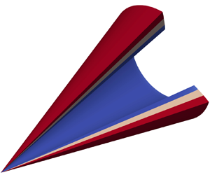

1. Introduction
The Taylor–Maccoll (T–M) equations were initially formulated to study supersonic flows over a cone (Busemann Reference Busemann1929; Taylor & Maccoll Reference Taylor and Maccoll1933). It is found, nonetheless, that the equations held not only for the external conical flow (ECF) but also for internal conical flows. Busemann (Reference Busemann1942, as cited in Grozdovskii Reference Grozdovskii1959; Mölder & Szpiro Reference Mölder and Szpiro1966) studied a conical flow with uniform inflow and outflow, known as the Busemann flow, using the T–M equations. In addition to the ECF and the Busemann flow, Grozdovskii (Reference Grozdovskii1959) presented two types of internal conical flows through a hodograph, which were later termed the internal conical flow of type A and B (ICFA and ICFB) by Mölder (Reference Mölder1967). The above solutions were also called the M- and W-flow, respectively, in recent studies by Mölder & Timofeev (Reference Mölder and Timofeev2022). The classic solutions, i.e. ECF, Busemann flow, ICFA and ICFB, are essentially the four primary solutions to the T–M equations that correspond to flows through the configurations depicted in figure 1 (Mölder Reference Mölder1967; Musa et al. Reference Musa, Huang, Jin, Mölder and Yu2023). These solutions consist of a uniform flow followed by an isentropic compression or expansion zone, with a conical shock in between. The ICFA and ICFB are additionally bounded by the singular lines, beyond which the solutions no longer obey the T–M equations. Further, the T–M equations can be extended beyond the calorically perfect gas. Lampe (Reference Lampe1994) extended the T–M equations to the thermal perfect gas and applied it to the ECF. Granik (Reference Granik1986) even attempted to construct the T–M equations for the relativistic gas.
The classic T–M solutions (Mölder Reference Mölder1967; Musa et al. Reference Musa, Huang, Jin, Mölder and Yu2023): (a) ECF, (b) Busemann flow, (c) ICFA and (d) ICFB.

The ECF is the most common and simplest of the four classic solutions and is widely studied analytically. Maccoll & Taylor (Reference Maccoll and Taylor1936) solved the T–M equations utilizing Taylor expansion to yield a lower-order solution, which was subsequently extended by Schwartz (Reference Schwartz1975) to a series solution with 30 terms. Moorthy (Reference Moorthy1986) constructed an approximation by assuming constant density in the ECF. By dropping the velocity component normal to the cone surface, Ishimatsu & Morishita (Reference Ishimatsu and Morishita2005) formulated an analytical solution for the hypersonic ECF, which is applicable to estimation in aero-optics (Yao et al. Reference Yao, Zhang, Zhang, Huang, Gan and Zhu2019; Gao et al. Reference Gao, Li, Yuan and Dong2022). In conjunction with Newton's hypersonic approximation, Forbes & Hindle (Reference Forbes and Hindle2019) improved the approach for conical flows with a wider range of cone half-angles.
For the ICFA and ICFB, the flows beyond the singular lines do not satisfy the T–M equations. In fact, the flow upstream of the trailing characteristics follows the ICFA, while the downstream portion departs from the T–M equations. Courant & Friedrichs (Reference Courant and Friedrichs1976) suggested that regular conical shock reflection does not exist in the ICFA, which was supported by theoretical analyses (Rylov Reference Rylov1990; Isakova et al. Reference Isakova, Kraiko, P'Yankov and Tillyayeva2012; Kraiko & Tillyaeva Reference Kraiko and Tillyaeva2014), as well as numerical and experimental results (Mölder et al. Reference Mölder, Gulamhussein, Timofeev and Voinovich1997; Timofeev et al. Reference Timofeev, Mölder, Voinovich, Hosseini and Takayama2001, as cited in Shoesmith et al. Reference Shoesmith, Mölder, Ogawa and Timofeev2018).
Theoretically, it is irrelevant to the existence of the supersonic T–M solution whether the downstream flow is self-similar or not. Mölder & Timofeev (Reference Mölder and Timofeev2022) studied the conical shock reflection in the Busemann flow by experimental and numerical means. The model in the study is a truncated Busemann intake whose trailing characteristics are laid downstream of the apex of the conical shock. Accordingly, it is feasible to apply the T–M theory to the practical design of supersonic intakes, where the streamtube generated by streamline tracing as the intake channel would essentially be part of the T–M solution that excludes the portion containing the singular points and lines. Furthermore, Shoesmith et al. (Reference Shoesmith, Mölder, Ogawa and Timofeev2018) obtained numerically a flow consisting of the ICFA, expansion flow and regular reflection portions by setting a cylinder at the axis in conjunction with the initial ICFA solution.
Although the T–M solutions may not cover the full flow field in some practical conical flows, they can still be regarded as the baselines representing fully or partially the real flows in typical configurations. Accordingly, the T–M equations have been widely applied to waverider and intake design (Ding et al. Reference Ding, Liu, Shen, Liu, Chen and Fu2017; Zuo & Mölder Reference Zuo and Mölder2019). Nonweiler (Reference Nonweiler1959) proposed a waverider configuration from wedge flow. Jones et al. (Reference Jones, Moore, Pike and Roe1968) then derived a waverider formally from the ECF, while Goonko, Mazhul & Markelov (Reference Goonko, Mazhul and Markelov2000) chose an internal compression flow as the basic flow for waverider design. Recently, following the analysis of the space-marching disturbances, Jiang et al. (Reference Jiang, Hu, Gao, Lee and Xue2017) and Hu et al. (Reference Hu, Jiang, Gao and Lee2018) proposed a fast design methodology for wedge-cone derived waveriders via a decomposition of the wedge-cone flow. The T–M equations can be applied to the reference conical flows as stated above, as well as their infinitesimal elements. Sobieczky, Dougherty & Jones (Reference Sobieczky, Dougherty and Jones1990) proposed the osculating cone method, where the waverider is derived from local ECFs on the normal planes to the prescribed shock (or equivalently, the osculating planes of the post-shock streamlines by assumption). Sobieczky et al. (Reference Sobieczky, Zores, Wang and Qian1997) and Rodi (Reference Rodi2005) extended the infinitesimal elementary flows on the osculating planes to other axisymmetric flows. The composition of different T–M solutions may not only be realized along the flow direction but also be feasible across the osculating planes. Jiang, Gao & Lee (Reference Jiang, Gao and Lee2015) proposed an osculating surface method, capable of transforming the infinitesimal flow from the ECF and wedge flow to the ICFA regime. All methods for waverider design described above rely on a prescribed shock, while the leading-edge cone method proposed by Li et al. (Reference Li, Jiang, Hu, Lee and Pi2023) employs a prescribed leading edge. T–M theory has also been frequently applied to airframe-propulsion integration design. Takashima & Lewis (Reference Takashima and Lewis1995) used the flow over a wedge-cone body as the basic flow to achieve airframe-propulsion integration. He & Ni (Reference He and Ni2011) and He et al. (Reference He, Le, Zhou, Mao and Wu2012) adopted the ICFA and associated downstream combinations as the elementary flow to furnish the airframe-propulsion integrated design.
The potential application of the Busemann solution to the design of supersonic intakes was suggested by Courant & Friedrichs (Reference Courant and Friedrichs1948, as cited in Mölder Reference Mölder2019). Mölder & Szpiro (Reference Mölder and Szpiro1966) then conducted a performance analysis on Busemann intakes by solving the T–M equations. The starting performances of a Busemann intake can be estimated via the Busemann solution in conjunction with the starting theory of propulsion inlets. Based on a simplified mass spillage model, Najafiyazdi et al. (Reference Najafiyazdi, Tahir, Timofeev and Mölder2007) derived an analytical criterion for starting flows in Busemann intakes. Similarly, Moradian et al. (Reference Moradian, Timofeev, Tahir and Mölder2014, Reference Moradian, Timofeev, Tahir and Mölder2015); Moradian, Timofeev & Tahir (Reference Moradian, Timofeev and Tahir2017) formulated the startability criteria through startability analyses on Busemann intakes with overboard spillage. In addition, their results also revealed that the Busemann intake designed from the Busemann flow with a strong shock could improve the startability. The Busemann intake is usually truncated in practice to reduce the frictional loss. O'Brien & Colville (Reference O'Brien and Colville2008) indicated that the ICFA could act as the leading edge condition of the truncated Busemann intake. You, Zhu & Guo (Reference You, Zhu and Guo2009), Zuo, Mölder & Chen (Reference Zuo, Mölder and Chen2021) and Zuo & Mölder (Reference Zuo and Mölder2022) presented several intake designs by combining various ICFA with truncated Busemann flows. As to the combined Busemann intake, Van Wie & Mölder (Reference Van Wie and Mölder1992) suggested the tandem of a Busemann intake and a cone. Luo (Reference Luo2019) designed an intake by integrating a wedge flow, a Busemann flow and an ECF.
During a century of studies on fundamental problems related to the T–M equations and associated applications on the aerodynamic design, only four classic solutions, i.e. ECF, Busemann, ICFA and ICFB, have been reported. In particular, among those solutions, only the ECF, Busemann, ICFA and their combinations are ever utilized in engineering design. One may expect, however, that other T–M solutions, together with their associated combinations, would also serve practical purposes. For example, the mass injection into the supersonic flow over a cone may induce an alternative type of conical flow distinct from the classic four (see § 4.2). In the present work, the T–M equations are studied from a different perspective. The elementary solutions to T–M equations are analysed and classified accordingly in § 2. Solutions containing shocks are then introduced, and the composite solutions of the associated elementary solutions are categorized in § 3. In § 4, two new solutions found in the present work and a shock-connected solution are discussed. Finally, the summary of the work is given in § 5.
2. Elementary solutions to the Taylor–Maccoll equations
In practical applications of the classic T–M solutions, boundary conditions must be imposed in addition to those derived from the equations. Specifically, the inlet of the ECF and the ICFA or the outlet of the Busemann flow and the ICFB are manually assigned as a uniform flow parallel to the axis. However, the integration of the T–M equations with respect to the polar angle (T–M integration) terminates naturally downstream of the ECF and ICFA, as well as upstream of the Busemann flow and ICFB. For the ECF, the integration of the streamline encounters the infinite discontinuity of the streamline equation. Alternatively, for the Busemann flow, ICFA and ICFB, the T–M integration terminates at the infinite discontinuity of the T–M equations, or in other words, the singular line, noting that the singular line in the Busemann flow corresponds exactly to the uniform inflow.
Leaving out the additional boundary conditions and taking the T–M equations as an initial value problem, a class of solutions can be obtained by direct integration, which is terminated by the infinite discontinuity both upstream and downstream. These solutions can be truncated in accordance with specific boundary conditions and combined with each other to form composite solutions. Thus, these solutions are termed the elementary solutions in this work. This section will focus on the preliminary analysis of elementary solutions to the T–M equations, whose corresponding solution domains are classified according to the critical surfaces in the pre-shock (§ 2.2) and post-shock (§ 2.3) domains.
2.1. Basic analysis of Taylor–Maccoll solutions
2.1.1. Basic properties of Taylor–Maccoll equations
The T–M equations are usually formulated on the polar coordinates, where the independent variable is the polar angle ( $\theta$). The dependent variables are the radial and circumferential components of the flow velocity (
 $u_r,u_\theta$) (Mölder Reference Mölder1967), either non-dimensionalized by the theoretically maximum speed (Maccoll & Taylor Reference Maccoll and Taylor1936) or the characteristic sonic speed (Grozdovskii Reference Grozdovskii1959). In this work, the square of the characteristic Mach number (
 $\lambda ^2$) and the flow inclination (
 $\psi$) are introduced as the dependent variables to simplify the expression of critical surfaces and facilitate the analysis. As shown in figure 2,
 $(x,y)$ are Cartesian coordinates, while
 $(r,\theta )$ are polar coordinates. Also,
 $\varphi$ and
 $\psi$ are the flow inclination with respect to the polar line and the axis, respectively, or the relative and absolute flow inclinations in short. The characteristic Mach number
 $\lambda$ can be related to the Mach number
 $M$ with
 \begin{equation} \lambda^2 = \frac{\gamma+1}{2/M^2 + (\gamma-1)}\in(0,\lambda^2_{lim}),\quad \lambda^2_{lim}=\lim_{M^2\to\infty}\lambda^2=\frac{\gamma+1}{\gamma-1}, \end{equation}
where  $\gamma$ is the specific heat ratio of the gas. By formulating the T–M equations in (
 $\lambda ^2,\psi,\theta$) space, we obtain (cf. Appendix A for details)
 $$\begin{gather} \frac{1}{2\lambda^2} \frac{\mathrm{d}\lambda^2}{\mathrm{d}\theta} =- \frac{\sin\psi}{\sin\theta} \frac{\sin\varphi}{1-M^2\sin^2\varphi}, \end{gather}$$
 $$\begin{gather}\frac{\mathrm{d}\psi}{\mathrm{d}\theta}=- \frac{\sin\psi}{\sin\theta} \frac{\cos\varphi}{1-M^2\sin^2\varphi}, \end{gather}$$
whose solution with initial point  $(\lambda ^2_0,\psi _0,\theta _0)$ can be expressed as
 $\boldsymbol {F}(\theta ;\lambda ^2_0,\psi _0,\theta _0)$. The streamline and its curvature are evaluated by solving the following equations:
 $$\begin{gather} \frac{\mathrm{d}\ln r}{\mathrm{d}\theta} = \cot\varphi, \end{gather}$$
 $$\begin{gather}\kappa = \frac{\sin\varphi}{r}\frac{\mathrm{d}\psi}{\mathrm{d}\theta}. \end{gather}$$
The coordinates for the T–M equations and T–M flow.

The solution to the T–M equations (2.2) and the streamline equation (2.3) with initial value  $\boldsymbol {\hat {x}}(\theta _0)=(\lambda ^2_0,\psi _0,\ln r_0)$ is denoted as
 $\boldsymbol {\hat {F}}(\theta ; \boldsymbol {\hat {x}}(\theta _0), \theta _0)$, where three intuitive properties, namely, the properties of evolution, reversal and symmetry, can be deduced.
Property 2.1 (Evolution)
Identical solutions can be obtained with different initial values on the solution,  $\boldsymbol {\hat {F}}(\theta ) = \boldsymbol {\hat {F}}(\theta ; \boldsymbol {\hat {x}}_0, \theta _0) = \boldsymbol {\hat {F}}(\theta ; \boldsymbol {\hat {F}}(\theta _1; \boldsymbol {\hat {x}}_0, \theta _0), \theta _1)$.
Property 2.2 (Reversal)
The flow direction of the T–M solution is reversible. The solutions with opposite initial velocities satisfy  $\boldsymbol {\hat {F}}(\theta ; \boldsymbol {\hat {x}}_0 + (0,\pm {\rm \pi},0), \theta _0) = \boldsymbol {\hat {F}}(\theta ; \boldsymbol {\hat {x}}_0, \theta _0) + (0,\pm {\rm \pi},0)$.
Property 2.3 (Symmetry)
The solutions with initial values symmetric to the lines  $(\varphi,\theta )=(k{\rm \pi} /2,{\rm \pi} /2)$ are of reflection symmetry
 \begin{equation} \left.\begin{gathered} \lambda^2({\rm \pi}-\theta; \boldsymbol{\hat{x}}_{sym}, {\rm \pi}-\theta_0) = \lambda^2(\theta; \boldsymbol{\hat{x}}_0, \theta_0)\\ k{\rm \pi}-\psi({\rm \pi}-\theta; \boldsymbol{\hat{x}}_{sym}, {\rm \pi}-\theta_0) = \psi(\theta; \boldsymbol{\hat{x}}_0, \theta_0)\\ r({\rm \pi}-\theta; \boldsymbol{\hat{x}}_{sym}, {\rm \pi}-\theta_0) = r(\theta; \boldsymbol{\hat{x}}_0, \theta_0). \end{gathered}\right\},\quad \boldsymbol{\hat{x}}_{sym} =(\lambda^2_0, k{\rm \pi}-\psi_0, \ln r_0). \end{equation}
Critical surfaces can be directly deduced from (2.2)–(2.4). Taking the derivatives in (2.2) to be zero, the equilibria ( $\sin \psi =0$) are yielded, which represent the uniform flows with
 $\psi =0$ or
 ${\rm \pi}$. The equilibria here are a collection of trivial solutions and denoted as
 $S_{equ} = \{(\lambda ^2,\varphi,\theta )\,|\,\sin \psi =0\}$. Taking the denominator in either equation (2.2), (2.3) to be zero, the infinite discontinuities for the specific equations are yielded. The integration of the T–M equations (2.2) will be terminated by the infinite discontinuity
 $M^2\sin ^2\varphi =1$, which is termed Mach discontinuity in this work and denoted as
 $S_{Ma} = \{(\lambda ^2,\varphi,\theta )\,|\,M^2\sin ^2\varphi =1\}$. Similarly, the integration of the streamline equation (2.3) can be terminated by the infinite discontinuity
 $\sin \varphi =0$, which is termed slip discontinuity and denoted as
 $S_{slip} = \{(\lambda ^2,\varphi,\theta )\,|\,\sin \varphi =0\}$. In addition, the surface
 $\cos \varphi =0$ consists of zero-curvature points (
 $\kappa =0$) for the streamlines of non-trivial solutions (
 $\sin \psi \neq 0$) and is denoted as
 $S_{\kappa =0} = \{(\lambda ^2,\varphi,\theta )\,|\,\cos \varphi =0\}$.
2.1.2. Mach discontinuity as a bound of the elementary solution
The critical surfaces and typical solutions are plotted both in the  $(\lambda ^2,\varphi,\theta )$ space and on the
 $(\lambda ^2,\varphi )$ plane for clarity (cf. figure 3). The slice of
 $S_{equ}$ varies linearly along the
 $\varphi$-axis as
 $\theta$ varies, while the slices of
 $S_{Ma}$ and
 $S_{slip}$ are independent of
 $\theta$. The slices of critical surfaces on the plane
 $(\lambda ^2,\varphi )$ will be utilized consistently in this work as they are more concise for illustration, as compared with those on the phase plane
 $(\lambda ^2,\psi )$.
(a) Mach discontinuity, equilibria and typical solutions in  $(\lambda ^2,\varphi,\theta )$ space; (b) slice of the surfaces and projection of the solutions on the
 $(\lambda ^2,\varphi )$ plane at
 $\theta =15^\circ$.

Apart from the trivial solutions on  $S_{equ}$, the integrations of the T–M equations along
 $\theta$ directed toward 0 and
 ${\rm \pi}$ are both terminated by
 $S_{Ma}$, at the corresponding terminal points marked with
 $\bigcirc$ and
 $\triangle$, respectively, in figure 3. Thus, the elementary solution is a T–M solution defined on an interval that cannot be extended across
 $S_{Ma}$. For clarity, the solution branches and terminal points are defined as follows.
Definition 2.1 (Lower/upper branches and terminal points)
The elementary solution  $\boldsymbol {F}(\theta ) =\boldsymbol {F}(\theta ;\lambda ^2_0,\psi _0,\theta _0)$ is defined on a maximal open interval
 $(\theta _l,\theta _u)\subset (0,{\rm \pi} )$. The portions of the solution
 $\boldsymbol {F}(\theta )$ defined on the interval, vis-à-vis,
 $(\theta _l,\theta _0]$ and
 $[\theta _0,\theta _u)$, are termed the lower and upper branches of the elementary solution, respectively.
The lower and upper terminal points are the limiting points of the lower and upper branches towards the Mach discontinuity. Symbolically,  $(\lambda ^2_{l,u},\psi _{l,u}) =\lim _{\theta \to \theta _{l,u}}\boldsymbol {F}(\theta )$ with
 $M^2_{l,u}\sin ^2\varphi _{l,u}=1$.
The leading and trailing characteristic curves of the elementary solution are tangent to the singular line at the terminal points since the relative flow inclination there is equal to the Mach angle, i.e.  $|\varphi _{l,u}|=\mu$. The Mach discontinuity can be split into two families of segments based on whether the characteristics are left or right running, (cf. figure 3b).
Definition 2.2 (Left-/right-running Mach discontinuity)
The Mach discontinuity which lies in the interval, vis-à-vis,  $\varphi \in (-{\rm \pi} /2+k{\rm \pi},k{\rm \pi} )$ or
 $\varphi \in (-{\rm \pi} +k{\rm \pi},-{\rm \pi} /2+k{\rm \pi} ),\ k\in \mathbb {Z}$, is termed a left- or right-running Mach discontinuity and denoted as
 $S_{Ma}^\pm$, respectively.
To illustrate the influence of the left- and right-running characteristics on the solution, numerical results of four cases are obtained by solving the axisymmetric Euler equations and presented in figure 4. Four cases are divided into two groups corresponding to two elementary solutions. Two cases of the same group share the same wall surface (the bold streamlines) and free-stream Mach number, which are provided by one elementary solution. The group in the left column (cf. figure 4a,b) is based on an elementary solution called degenerate conical flow (DCF, later introduced in § 2.3.2). Alternatively, the reference T–M solution for the group in the right column (cf. figure 4c,d) is a Busemann flow. The leading characteristics are left running for the DCF solution, indicating that the disturbance induced by the wall should propagate away from the axis. Thus, the external flow (figure 4a) behaves as a conical expansion flow. In contrast, the internal flow (figure 4b) is not conical, because it is affected by the right-running characteristics, which is not expected in the DCF solution. Alternatively, since the leading characteristics are right running for the Busemann solution, the internal flow (figure 4d) behaves as the Busemann flow, while the external flow (figure 4c) does not satisfy the T–M equations. The characteristic curves at the singular line determine whether a T–M solution is internal or external.
(a) External and (b) internal flow for a DCF solution. (c) External and (d) internal flow for a Busemann solution. Solid lines are contour lines of Mach number. Dashed lines are polar lines. The dot-dash-dot line is the axis.

Since the elementary solution is bounded by  $S_{Ma}$,
 $S_{Ma}$ naturally divides the solution domain into the pre-/post-shock subdomains characterized by the Mach number corresponding to the
 $\theta$-component of the velocity,
 $M\sin \varphi$. Symbolically, these domains can be specified as
 \begin{equation} D_{pre}=\{(\lambda^2,\varphi,\theta)\,|\,M^2\sin^2\varphi>1\},\quad D_{post}=\{(\lambda^2,\varphi,\theta)\,|\,M^2\sin^2\varphi<1\}. \end{equation}
Note that the shock here refers to the shock encountered in a T–M solution, which is in coincidence with the polar line. Secondary shock can emerge if the post-shock flow is supersonic. However, the secondary shock will not be located on a polar line, and the flow downstream does not satisfy the T–M equations. A typical example is the supersonic flow over a biconic body. The elementary solutions in the pre-/post-shock domains are presented in the following subsections, while discussions on shock solutions are reserved for § 3.
2.2. Pre-shock domain
2.2.1. Symmetric subdomains
The pre-shock domain is cut by the Mach discontinuity into periodically spanned unconnected subdomains, in which the  $k$th subdomain can be denoted as
 \begin{equation} D_{{pre},k} = D_{pre}\cap \{(\lambda^2,\varphi,\theta)\,|\,\varphi\in((k-1){\rm \pi},k{\rm \pi}),\ k\in\mathbb{Z}\}. \end{equation}
Due to the reversible nature of the T–M equations, the elementary solutions in  $D_{{pre},k}$ are the same as those in
 $D_{{pre},k+1}$, except that the reversal in the flow direction. In addition, the equilibria (
 $\psi =k{\rm \pi}$) are those elementary solutions that pass through the lines
 $(\varphi,\theta )=((2k-1){\rm \pi} /2,{\rm \pi} /2)$, respectively. The symmetry property enables
 $S_{equ}$ to subdivide
 $D_{{pre},k}$ into two symmetric subdomains for each
 $k$, which are named pre-shock domains I and II, which can be specified symbolically as
 $$\begin{gather} D_{pre,I} = D_{pre}\cap \{(\lambda^2,\varphi,\theta)\,|\, \varphi\in((k-1){\rm \pi},k{\rm \pi}-\theta),\ k\in\mathbb{Z}\}, \end{gather}$$
 $$\begin{gather}D_{pre,II} = D_{pre}\cap \{(\lambda^2,\varphi,\theta)\,|\, \varphi\in(k{\rm \pi}-\theta,k{\rm \pi}), k\in\mathbb{Z}\}. \end{gather}$$
Note that the portions of pre-shock solutions in  $D_{pre,I}$ for
 $\theta \in ({\rm \pi} /2,{\rm \pi} )$ and those in
 $D_{pre,II}$ for
 $\theta \in (0,{\rm \pi} /2)$ are mutually correspondent. The pre-shock solutions with initial points spanned on
 $\theta \in (0,{\rm \pi} /2]$ can represent the solutions in the entire pre-shock domain.
2.2.2. Divergence bound
Figure 5 depicts the elementary solutions in  $D_{pre,I}$ for initial values
 $\lambda ^2_0=4,\theta _0=15^\circ$ with varying
 $\varphi _0$ in
 $(\lambda ^2,\varphi,\theta )$ space and on the
 $(\lambda ^2,\varphi )$ plane. Projections of the corresponding convergent, critical and divergent solutions on the
 $(\varphi,\theta )$ and
 $(\lambda ^2,\theta )$ planes are shown in figure 6. All three types of solutions persist in a similar trend, with an essential difference stemming from the upper terminal point. For the usual convergent solution (here,
 $\varphi _0=-30^\circ$),
 $\lambda ^2_u<\lambda ^2_{lim},\psi _u=0$, the upper terminal point lies on the equilibria, indicating a uniform inflow at the singular line. For the critical solution (
 $\varphi _0=-48.61^\circ$),
 $\lambda ^2_u=\lambda ^2_{lim},\psi _u=0$, the upper terminal point lies on the edge of the equilibria, which coincides with the limiting characteristic Mach number, implying a uniform inflow with the maximum speed. For the divergent solution (
 $\varphi _0=-60^\circ$),
 $\lambda ^2_u=\lambda ^2_{lim},\psi _u<0$, the upper terminal point retains the maximum speed, but no longer lies on the equilibria, nor does it pertain to a uniform inflow.
(a) Divergence bound and typical solutions in  $(\lambda ^2,\varphi,\theta )$ space; (b) slice of the surfaces and projection of the solutions on the
 $(\lambda ^2,\varphi )$ plane at
 $\theta =15^\circ$.

(a) Values of  $\varphi$ and (b)
 $\lambda ^2$ varying with
 $\theta$ for convergent, critical and divergent solutions.

The collection of all possible critical solutions mentioned above can be defined as the divergence bound, which divides the pre-shock domain into convergent/divergent domains.
Definition 2.3 (Divergence bound)
The divergence bound I (or II) is the collection of all possible elementary solutions in  $D_{pre,I}$ (or
 $D_{pre,II}$), whose upper (or lower) terminal points lie on
 $S_{equ}$ and reach exactly the limit of characteristic Mach number
 $\lambda _{lim}$. Symbolically, the divergence bounds can be expressed as follows:
 $$\begin{gather} S_{div,I} = \{(\lambda^2,\varphi,\theta)\,|\, \boldsymbol{F}({\rm \pi}; \lambda^2,\varphi,\theta) = (\lambda^2_{lim},(k-1){\rm \pi}),\ k\in\mathbb{Z}\}, \end{gather}$$
 $$\begin{gather}S_{div,II} = \{(\lambda^2,\varphi,\theta)\,|\, \boldsymbol{F}(0; \lambda^2,\varphi,\theta) = (\lambda^2_{lim},k{\rm \pi}),\ k\in\mathbb{Z}\}. \end{gather}$$
The domain enclosed by  $S_{Ma}$ and
 $S_{div}$ is termed convergent domain and denoted as
 $D_{conv}$, which is also divided into symmetric subdomains
 $D_{conv,I}$ and
 $D_{conv,II}$ by the equilibria. Similarly, the complementary domain of
 $D_{conv,I/II}$ in
 $D_{pre,I/II}$ is termed divergent domain I/II and denoted as
 $D_{div,I/II}$, respectively.
2.2.3. Inflection bound in pre-shock domain
A three-dimensional plot of the elementary solutions for initial values  $\lambda ^2_0=5.0,\theta _0=15^\circ$ with varying
 $\varphi _0$, together with the projection on the
 $(\lambda ^2,\varphi )$-plane are shown in figure 7. The trend of the solutions can be observed from the projections on the
 $(\varphi,\theta )$- and
 $(\lambda ^2,\theta )$-planes as depicted in figure 8. Three types of solutions can be seen in this test case, namely, inflectional, critical and non-inflectional. The streamline of the inflectional solution (here
 $\varphi _0=167.1^\circ$) always consists of an inflection point, while those of the critical solution (
 $\varphi _0=167.135^\circ$) and the non-inflectional solution (
 $\varphi _0=167.2^\circ$) do not. These three types of solutions are close to each other for
 $\theta \le \theta _0$, and then the inflectional and non-inflectional ones bend away from the opposite sides of the critical solution as
 $\theta$ increases (cf. figure 8). The corresponding flow fields are illustrated in figure 9, where the usual inflectional solution (cf. figure 9a) is similar to the classic Busemann flow. The lower/upper branches of the inflectional solution terminate, respectively, at
 $S_{Ma}^\pm$ with
 $\varphi _u<{\rm \pi} /2<\varphi _l$, indicating the transition from internal compression to external compression. The critical solution terminates at exactly the sonic point
 $\lambda ^2_u=1,\varphi _u={\rm \pi} /2$, representing the flow with maximum isentropic compression that can be given by the T–M equations theoretically. The upper and lower branches of the non-inflectional solution both terminate at
 $S_{Ma}^+$, where
 ${\rm \pi} /2<\varphi _u<\varphi _l$.
(a) Inflection bound and typical solutions in  $(\lambda ^2,\varphi,\theta )$ space; (b) slice of the surfaces and projection of the solutions on the
 $(\lambda ^2,\varphi )$ plane at
 $\theta =15^\circ$.

(a) Values of  $\varphi$ and (b)
 $\lambda ^2$ varying with
 $\theta$ for inflectional, critical and non-inflectional solutions.

(a) Inflectional, (b) critical and (c) non-inflectional solutions with  $\lambda ^2_0=5.0,\theta _0=15^\circ$ and varying
 $\varphi _0$.

The derivative  $\mathrm {d}\varphi /\mathrm {d}\lambda ^2$ at
 $\cos \varphi =0$ in the domain
 $D_{pre,II}$
 \begin{equation} \left.\frac{\mathrm{d}\varphi}{\mathrm{d}\lambda^2}\right|_{\cos\varphi=0} = \left.-\frac{\mathrm{d}\theta}{\mathrm{d}\lambda^2}\right|_{\cos\varphi=0}>0, \end{equation}
which indicates that the inflectional solution goes across  $S_{\kappa =0}$ only once, rather than passing through it repeatedly or touching it tangentially. As a result, the terminal points of the inflectional solution will lie on different segments of
 $S_{Ma}$, while the non-inflectional solution is supported by the same one, either
 $S_{Ma}^+$ or
 $S_{Ma}^-$. For the critical solution, one of its terminal points is exactly the split point of
 $S_{Ma}^\pm$. Thus, the inflectional and non-inflectional solutions can be determined according to the location of the terminal point.
Definition 2.4 (Inflection bound in the pre-shock domain)
The collection of the elementary solutions in  $D_{pre,I}$, whose lower branches terminate at exactly the zero-curvature point, is termed inflection bound I and denoted as
 $S_{inflect,I}$.
Similarly, the collection of the elementary solutions in  $D_{pre,II}$, whose upper terminal points are sonic, is termed inflection bound II and denoted as
 $S_{inflect,II}$. Symbolically
 $$\begin{gather} S_{inflect,I} = D_{pre}\cap \{(\lambda^2,\varphi,\theta)\,|\, \boldsymbol{F}(\theta_l; \lambda^2,\varphi,\theta) = (1.0,(2k-1){\rm \pi}/2),\ k\in\mathbb{Z}\}, \end{gather}$$
 $$\begin{gather}S_{inflect,II} = D_{pre}\cap \{(\lambda^2,\varphi,\theta)\,|\, \boldsymbol{F}(\theta_u; \lambda^2,\varphi,\theta) = (1.0,(2k-1){\rm \pi}/2),\ k\in\mathbb{Z}\}. \end{gather}$$
The domain enclosed by  $S_{Ma}$,
 $S_{equ}$,
 $S_{inflect,I}$ (or
 $S_{inflect,II}$) and the surface
 $\lambda ^2=\lambda ^2_{lim}$ is termed inflection domain I (or II) and denoted as
 $D_{inflect,I}$ (or
 $D_{inflect,II}$). The complementary domain of
 $D_{inflect,I/II}$ in
 $D_{pre,I/II}$ is termed non-inflection domain I/II and denoted as
 $D_{non\textrm {-}inflect,I/II}$.
The intersection of  $S_{div}$ and
 $S_{inflect}$ divides
 $S_{pre}$ into four subdomains: the convergent inflectional domain (Busemann domain,
 $D_{Bu}$), the convergent non-inflectional domain (
 $D_{non\textrm {-}inflect,Bu}$), the divergent inflectional domain (
 $D_{inflect,div}$) and the divergent non-inflectional domain (
 $D_{non\textrm {-}inflect,div}$).
2.3. Post-shock domain
2.3.1. Symmetric subdomains
The post-shock domain is the connected domain across the entire  $\varphi$-axis with
 $\lambda ^2<\lambda ^2_{Ma}$. To facilitate the analysis, the post-shock domain is firstly divided into subdomains according to the property of symmetry. The elementary solutions passing through the lines
 $(\varphi,\theta )=((2k-1){\rm \pi} /2,{\rm \pi} /2)$ are exactly the equilibria,
 $\psi =k{\rm \pi}$, which divide the post-shock domain into periodical subdomains as
 \begin{equation} D_{{post},k} = D_{post}\cap \{(\lambda^2,\varphi,\theta)\,|\,\psi\in((k-1){\rm \pi},k{\rm \pi}),\ k\in\mathbb{Z}\}. \end{equation}
The elementary solutions passing through the lines  $(\varphi,\theta )=(k{\rm \pi},{\rm \pi} /2)$ are termed symmetry bound and denoted as
 $S_{sym}$ (cf. figure 10)
 \begin{equation} S_{sym} = \{(\lambda^2,\varphi,\theta)\,|\,(\lambda^2,\varphi) = \boldsymbol{F}(\theta; \lambda^2_0,k{\rm \pi},{\rm \pi}/2),\lambda^2_0\in(0,\lambda^2_{lim}),\ k\in\mathbb{Z}\}. \end{equation}
The symmetry bound in each  $D_{{post},k}$ can further subdivide it into two symmetric portions, the post-shock domains I and II, which can be specified symbolically as follows:
 $$\begin{gather} D_{post,I} = D_{post}\cap \{(\lambda^2,\varphi,\theta)\,|\, \varphi\in(k{\rm \pi}-\theta,\varphi_{sym}),\ k\in\mathbb{Z}\}, \end{gather}$$
 $$\begin{gather}D_{post,II} = D_{post}\cap \{(\lambda^2,\varphi,\theta)\,|\, \varphi\in(\varphi_{sym},(k+1){\rm \pi}-\theta),\ k\in\mathbb{Z}\}. \end{gather}$$
As a result, the portions of post-shock solutions  $D_{post,I}$ for
 $\theta \in ({\rm \pi} /2,{\rm \pi} )$ are equivalent to those in
 $D_{post,II}$ for
 $\theta \in (0,{\rm \pi} /2)$. The analysis performed in
 $D_{post}$ for
 $\theta \in (0,{\rm \pi} /2]$ would be representative for the entire post-shock domain.
(a) Critical surfaces and typical solutions in  $(\lambda ^2,\varphi,\theta )$ space; (b) slice of the surfaces and projection of the solutions on the
 $(\lambda ^2,\varphi )$ plane at
 $\theta =15^\circ$.

The elementary solutions on  $D_{{sym}}$ are literally symmetric, as shown in figure 11(b). Also, the solutions above and below the symmetry bound (cf. figure 11a,c) are symmetric to each other. The flow above the slipstream resembles the classic ECF solution, while the flow below differs entirely from the nature of those four classic solutions. Thus, the corresponding solution branches can be abbreviated as the ECF and the inner flow of ECF (IECF), respectively.
The ECF–IECF solutions (a) with  $\theta _0<\theta _{sym}$, (b) on
 $S_{sym}$ and (c) with
 $\theta _0>\theta _{sym}$.

2.3.2. Degeneration bound
The elementary solutions for  $\varphi _0=150^\circ,\theta _0=15^\circ$ by varying
 $\lambda ^2_0$ show a similar trend as depicted in figures 12 and 13, where the essential difference appears at the upper terminal points. The elementary solution that passes through the slip discontinuity is split into the ECF and IECF branches (cf. figure 14c). However, unlike the classic ECF solution, the ECF branch here contains an inflection point. As
 $\lambda ^2_0$ increases, the slipstream moves toward the axis, and the IECF branch shrinks accordingly. When
 $\lambda ^2_0$ reaches a critical value, the slipstream coincides with the axis while the IECF branch disappears (cf. figure 14b).
(a) Critical surfaces and typical solutions in  $(\lambda ^2,\varphi,\theta )$ space; (b) slice of the surfaces and projection of the solutions on the
 $(\lambda ^2,\varphi )$ plane at
 $\theta =15^\circ$.

(a) Values of  $\varphi$ and (b)
 $\lambda ^2$ varying with
 $\theta$ for degenerate, critical and non-degenerate solutions.

(a) The DCF, (b) critical and (c) ECF–IECF solutions with  $\varphi _0=150^\circ,\theta _0=15^\circ$ and varying
 $\lambda ^2_0$.

The elementary solution that consists of ECF and IECF branches and passes through the slip discontinuity can be stated as the non-degenerate solution in contrast to the solution for the DCF, whose IECF branch disappears. In general, the upper terminal points of the degenerate and critical solutions are located exactly on the equilibria (cf. figure 13a), implying uniform flow (cf. figure 14a,b). In particular, all the critical solutions approach tangentially to the singular points  $(1,(2k+1){\rm \pi} /2,{\rm \pi} /2)$. The collection of the above critical solutions can be defined as the degeneration bound, which separates the degenerate solutions from the non-degenerate ones.
Definition 2.5 (Degeneration bound)
The collection of the elementary solutions in  $D_{post}$, which are terminated by and tangent to
 $S_{Ma}$ at the singular points
 $(1,(2k+1){\rm \pi} /2,{\rm \pi} /2)$, is termed the degeneration bound and denoted as
 $S_{degen}$
 \begin{equation} S_{degen} = D_{post}\cap\{(\lambda^2,\varphi,\theta)\,|\, \boldsymbol{F}({\rm \pi}/2; \lambda^2,\varphi,\theta)= (1.0,(2k+1){\rm \pi}/2)\}. \end{equation}
The domain enclosed by  $S_{Ma}$,
 $S_{equ}$ and
 $S_{degen}$ can be defined as the degenerate domain and denoted as
 $D_{DCF}$. The associated complementary domain in
 $D_{post}$ is termed non-degenerate domain and denoted as
 $D_{CF}$.
Accordingly, the degeneration bound divides the post-shock domain into non-degenerate and degenerate domains consisting of elementary solutions with and without the IECF branch, respectively. The non-degenerate domain can be subdivided further into subdomains corresponding to the ECF and IECF branches, considering that the streamline of ECF–IECF solutions is not continuous at  $S_{slip}$. The IECF domain is enclosed by
 $S_{Ma}$,
 $S_{slip}$ and
 $S_{sym}$ and denoted as
 $D_{IECF}$, while the ECF domain is the complementary domain of
 $D_{IECF}$ in
 $D_{CF}$ and denoted as
 $D_{ECF}$. The associated subsets of
 $D_{ECF}$ in
 $D_{post,I/II}$ are denoted as
 $D_{ECF,I/II}$.
2.3.3. Sonic bound
The local minimum of  $\lambda ^2$ for the elementary solution in
 $D_{post}$ is located at
 $\mathrm {d}\lambda ^2/\mathrm {d}\theta =0$, or
 $\sin \varphi =0$. Thus, elementary solutions passing through the sonic points on the slip discontinuity are supersonic elsewhere. Accordingly, the collection of the above solutions is termed a sonic bound and denoted as
 $S_{sonic}$. Symbolically,
 \begin{equation} S_{sonic} = \{(\lambda^2,\varphi,\theta)\,|\,(\lambda^2,\varphi) = \boldsymbol{F}(\theta; 1.0,k{\rm \pi},\theta_0),\theta_0\in(0,{\rm \pi}),\ k\in\mathbb{Z}\}. \end{equation}
The elementary solutions on  $S_{degen}$ terminate exactly at the sonic point
 $(1,(2k+1){\rm \pi} /2,{\rm \pi} /2)$, among which the sonic equilibrium has the minimum speed. Thus, the solutions in
 $D_{DCF}$ are supersonic. As illustrated in figure 15,
 $S_{sonic}$ and
 $S_{degen}$ divide
 $D_{post}$ into the transonic domain
 $D_{trans}$ and the supersonic domain
 $D_{super}$. Since the post-shock solutions with inflection points (cf. figure 31c) must intersect with
 $S_{\kappa =0}$, where the intersection points are subsonic, all the elementary solutions in
 $D_{super}$ are non-inflectional.
(a) Critical surfaces in  $(\lambda ^2,\varphi,\theta )$ space and (b) their slices at
 $\theta =15^\circ$.

3. Shock-connected solutions to the Taylor–Maccoll equations
There is always a shock in the four classic solutions to the T–M equations, where the pre- or post-shock flow appears as part of an elementary solution or a trivial solution, i.e. the uniform flow. The shock discontinuity cannot be obtained from direct integration of the T–M equations (2.2). Rather, the shock serves as the termination condition for the elementary solution, which does not alter the distribution of flow parameters along the polar angle. Thus, a T–M solution with a shock can be regarded as a combination of two elementary solution branches sharing a common shock as their initial stations. Accordingly, the above combined solution can be named the shock-connected solution.
In the shock-connected solution, the Rankine–Hugoniot relation can be represented in terms of the pre- and the post-shock parameters as
 $$\begin{gather} \frac{\tan\varphi_1}{\tan\varphi_2}= \frac{(\gamma+1)M_1^2\sin^2\varphi_1} {2+(\gamma-1)M_1^2\sin^2\varphi_1}, \end{gather}$$
 $$\begin{gather}M_2^2\sin^2\varphi_2 = \frac{2+(\gamma-1)M_1^2\sin^2\varphi_1} {2\gamma M_1^2\sin^2\varphi_1 - (\gamma-1)}, \end{gather}$$
where the subscripts 1, 2 denote the points on the opposite sides of a shock. Note that the formula remains valid after the swap of the subscripts. The details of the manipulation are given in Appendix B. Let the shock be located at  $\theta =\theta _{s}$, then a pair of points on both sides of the shock,
 $(\lambda ^2_{1},\varphi _{1},\theta _{s})$ and
 $(\lambda ^2_{2},\varphi _{2},\theta _{s})$, can produce a pair of elementary solutions,
 $\boldsymbol {F}_{1,2}(\theta ) =\boldsymbol {F}(\theta ; \lambda ^2_{1,2},\varphi _{1,2},\theta _{s})$, whose branches can be combined to form T–M solutions with a shock. One branch (upper/lower) of the pre-shock solution can be combined with the other branch (lower/upper) of the post-shock solution by the shock. The nature of some particular combinations with trivial uniform solutions corresponding to the four classic solutions will be discussed firstly in § 3.1. Then, combinations of general T–M solutions will be analysed in § 3.2.
3.1. Classic solutions to Taylor–Maccoll equations
Recall that the equilibrium surface  $S_{equ}$ is a plane consisting of trivial solutions. The mapping of the shock relations (3.1), (3.2) brings
 $S_{equ}$ to a parametric curvilinear surface, called the shock opposite of equilibria and denoted as
 $S'_{equ}$, which represents the pre-/post-shock state on the opposite side of a shock encountered in a post-/pre-shock uniform flow. Thus, conversely, the pre-/post-shock solution integrated from any point on
 $S'_{equ}$ corresponds to a uniform post-/pre-shock solution, respectively. In other words, the non-trivial solution branches of the four classic solutions, i.e. the ECF, Busemann, ICFA and ICFB branches, are either tangent to or intersect with
 $S'_{equ}$ in the space
 $(\lambda ^2,\varphi,\theta )$.
In addition, the projection of  $S'_{equ}$ on the
 $(\lambda ^2,\varphi )$ plane contains all possible pre-/post-shock states corresponding to the post-/pre-shock state on
 $(0,\lambda ^2_{lim})\times ((k-1){\rm \pi},k{\rm \pi} )$, which indicates that shock solutions cannot exist if the post-shock state
 $(\lambda ^2,\varphi )$ is outside the boundary of the projection, or symbolically
 \begin{equation} \lambda^2 \le \frac{\gamma^2-1}{(\gamma^2+1) - 2\gamma\cos2\varphi}. \end{equation}
3.1.1. Classic solutions with uniform outflow
The collection of the elementary solutions tangent to  $S'_{equ}$ (cf. figure 16a) is termed the classic Busemann bound and denoted
 $S_{cBu}$. The elementary solutions in
 $D_{pre}$ outside
 $S_{cBu}$ do not intersect with
 $S'_{equ}$, which implies that the classic solutions with uniform outflows, i.e. the classic Busemann and ICFB solutions, may not exist for the present case. In addition, each elementary solution on
 $S_{cBu}$ is tangent to
 $S'_{equ}$, corresponding to one uniform outflow. Every elementary solution interior to
 $S_{cBu}$ intersects with
 $S'_{equ}$ at two points, which produces two types of shock-connected solutions with strong and weak shocks, respectively. The numerical results reveal that
 $S_{cBu}$ does not intersect with
 $S_{inflect}$, and the domain consisting of the classic pre-shock solutions is contained in
 $D_{inflect}$. Hence, there exists an inflection point upstream of the shock in the classic Busemann flow, which is consistent with the conclusion given by Mölder (Reference Mölder2019).
(a) Classic Busemann bound and elementary solutions in  $(\lambda ^2,\varphi,\theta )$ space. Slices of critical surfaces and projection of the solutions on the
 $(\lambda ^2,\varphi )$ plane at (b)
 $\theta =15^\circ$, (c)
 $\theta =78.56^\circ$.

The combinations of the upper pre-shock branches and the lower post-shock branches in figure 16(b,c) are illustrated in figure 17(a,b). It is seen that the same pre-shock solution may be connected to different uniform post-shock flows with shocks of different intensities and locations. Here, the pre-shock solution is the same in the sense that the pre-shock branches that split at different shock locations share the same elementary solution.
Classic Busemann solutions with a (a) weak and (b) strong shock based on the same pre-shock solution.

3.1.2. Classic solutions with uniform inflow
Post-shock elementary solutions cannot approach tangentially to  $S'_{equ}$. They rather intersect with
 $S'_{equ}$ at a single point or emerge without intersection. Then, the boundary of
 $S'_{equ}$ (
 $\partial S'_{equ}$), determines the existence of the classic post-shock solution. Accordingly, the collection of the elementary solutions integrated from the points on the boundary is termed the classic ECF bound and denoted as
 $S_{cECF}$. In addition, the elementary solutions integrated from the points on
 $S'_{equ}$ which satisfy the shock detachment condition (B6) turn out to be exactly the detached solution of classic ECF type. Likewise, the collection of the above elementary solutions can be termed the detachment bound and denoted as
 $S_{detach}$.
The bounds  $S_{cECF}$ and
 $S_{detach}$ are illustrated in figure 18. The elementary solutions outside
 $S_{cECF}$ or on the right of
 $S_{degen}$ do not intersect with
 $S'_{equ}$, indicating that the classic solutions with uniform inflow, i.e. classic ECF and ICFA solutions, do not exist. The domain enclosed by
 $S_{cECF}$ can be subdivided further by
 $S_{detach}$ into subdomains for classic solutions with strong (left side) and weak (right side) shocks. Figure 19 depicts two types of ECF branches integrated downstream of strong and weak shocks, respectively, with the same uniform pre-shock inflow.
(a) Classic ECF bound, detachment bound and elementary solutions in  $(\lambda ^2,\varphi,\theta )$ space. Slices of critical surfaces and projection of the solutions on the
 $(\lambda ^2,\varphi )$ plane at (b)
 $\theta =15^\circ$, (c)
 $\theta =42.5^\circ$, (d)
 $\theta =87.14^\circ$.

Classic ECF solutions with a (a) weak and (b) strong shock under the same inflow velocity and cone half-angle.

3.1.3. Classic solutions as solution branches
A classic solution is a combination of two solution branches sharing a common shock as their initial stations. One branch shows the features of classic solutions, while the other is part of the equilibria. As illustrated in figure 20, with a pre-shock elementary solution in  $D_{pre}$ and its corresponding trivial solution in
 $D_{post}$, two pairs of different branches can be obtained to form two classic solutions. Specifically, the lower branch of the pre-shock solution can be combined with the upper branch of the post-shock equilibria to form the classic ICFB solution (cf. figure 20b), while the upper pre-shock branch and the lower post-shock branch form the classic Busemann solution (cf. figure 20c). Similarly, for the shock-connecting solution with a post-shock solution in
 $D_{post}$ and its corresponding pre-shock trivial solution (cf. figure 21), the upper branch of the post-shock solution is part of the classic ICFA solution (figure 21b), and the lower one is part of the classic ECF solution (figure 21c).
(a) Branches of the elementary solutions. Classic (b) ICFB solution (dashed lines in (a)) and (c) Busemann solution (solid lines in (a)).

(a) Branches of the elementary solutions. Classic (b) ICFA solution (dashed lines in (a)) and (c) ECF solution (solid lines in (a)).

In summary, the four classic solutions are combinations of branches extracted from two pairs of elementary solutions. The classic Busemann and ICFB solutions belong to one, while the classic ECF and ICFA solutions belong to the other. Further, following notations of the four classic solutions, the branch of solutions in  $D_{Bu}$ with uniform flows can be denoted as the Busemann branch, and the remaining branch the ICFB branch. Meanwhile, the branch of solutions that approaches
 $S_{slip}$ in
 $D_{ECF}$ can be denoted as the ECF branch, and the opposite branch is denoted as the ICFA branch.
3.2. Elementary solutions connected by a shock
The classic solutions are special cases of shock-connected solutions, where one of the pre- and post-shock elementary solutions is a trivial solution. In general, for a shock located at  $\theta =\theta _s$, the branches integrated from any pre-shock point (
 $\lambda ^2_{pre},\varphi _{pre},\theta _{s}$) can be connected with branches integrated from the corresponding post-shock point (
 $\lambda ^2_{post},\varphi _{post},\theta _{s}$) in accordance with the shock relations (3.1) and (3.2), to form a set of shock-connected solutions. The types of these elementary solutions are determined by the locations of the pre- and post-shock points. The shock plane,
 $S_{\theta =\theta _{s}}=\{(\lambda ^2,\varphi,\theta )\,|\,\theta =\theta _s\}$, where the pre- and post-shock points are located, is divided into several regions by the critical surfaces. Thus, the possible types of shock-connected solutions can be determined by investigating the topology of the regions.
3.2.1. Critical points for supersonic shock-connected solutions
Analogously to the shock opposite of equilibria, the mapping of the shock relations (3.1) and (3.2) can bring the critical surfaces defined in § 2 to parametric curvilinear surfaces, called the shock-opposite surfaces and denoted as  $S'$. The shock-opposite domains can be defined similarly and denoted as
 $D'$. Note that the shock-opposite surfaces are no longer collections of elementary solutions. Instead, they serve only as the references where the pair of pre- and post-shock points are located on
 $S_{\theta =\theta _{s}}$. In other words, the topology of the critical surfaces together with their associated shock opposites determine which pairs of pre- and post-shock subdomains
 $D_{1,2}$ can be connected for a shock located at
 $\theta =\theta _s$, or symbolically,
 $D'_1\cap D_2\cap S_{\theta =\theta _{s}}\ne \varnothing$.
To avoid a lengthy discussion, here, efforts will be focused on the combination with elementary solutions in  $D_{super}$, and the symbols introduced before will be used extensively (cf. Appendix C for the nomenclature). Figure 22 depicts the slices of most critical surfaces and their associated shock opposites at critical shock locations. The topologies on different slices are significantly distinct from each other. Thus, the permissible shock-connected solution varies correspondingly with respect to the variation of
 $\theta _{s}$.
Critical surfaces (solid lines) and their shock opposite (dotted lines) on  $S_{\theta =\theta _{s}}$. The relevant subdomains on the critical slice are filled with different colours. The dashed arrows indicate the direction the intersection curves move as
 $\theta$ increases. Panels show (a)
 $\theta _s=23.41^{\circ }$, (b)
 $\theta _s=27.8^{\circ }$, (c)
 $\theta _s=55.35^{\circ }$, (d)
 $\theta _s=58.92^{\circ }$, (e)
 $\theta _s=63.77^{\circ }$, (f)
 $\theta _s=66.85^{\circ }$.

As illustrated in figure 22, there are three relevant subdomains in  $D_{post}$ for
 $\theta \in (0,90^\circ ]$, i.e.
 $D_{super,ECF,I}$,
 $D_{super,IECF}$ and
 $D_{DCF}$;
 $D'_{super,ECF,I}$ behaves as a simply connected region contained in
 $D_{inflect,I}\cup D_{pre,II}$ on
 $S_{\theta =\theta _s}$ until
 $\theta _{s}$ reaches
 $58.92^\circ$. On
 $S_{\theta =58.92^\circ }$,
 $S_{sonic}$ touches
 $S_{Ma}$ and
 $D_{super,ECF,I}$ is split into two separate portions (cf. figure 22d), among which the smaller portion near the sonic equilibrium shrinks quickly as
 $\theta _s$ increases. When
 $\theta _{s}>66.85^\circ$,
 $D'_{super,ECF,I}$ retreats from
 $D_{inflect,div,I}$ (cf. figure 22f). In addition, the larger portion of
 $D'_{super,ECF,I}$ also retreats from
 $D_{Bu,I}$ and becomes contained in
 $D_{pre,II}$, while the smaller portion still intersects with
 $D_{Bu,I}$.
The shock-opposite subdomain  $D'_{super,IECF}$ is contained in
 $D_{non\textrm {-}inflect,div,I}$ initially. As
 $\theta _{s}$ increases,
 $D'_{super,IECF}$ begins to intersect with
 $D_{inflect,div,I}$,
 $D_{non\textrm {-}inflect,Bu,I}$ and
 $D_{Bu,I}$ at
 $\theta _{s}=23.41^\circ$,
 $55.35^\circ$,
 $63.77^\circ$, respectively (cf. figure 22a,c,e). The shock-opposite subdomain
 $D'_{DCF}$ intersects with
 $D_{inflect,I}$ initially. As
 $\theta _{s}$ increases,
 $D'_{DCF}$ retreats from
 $D_{inflect,div,I}$ and becomes contained in
 $D_{Bu,I}$ at
 $\theta _{s}=27.87^\circ$ (cf. figure 22b). As illustrated also in figure 22(b),
 $D_{conv,I}$ and
 $D_{non\textrm {-}inflect,I}$ begin to intersect with each other and form
 $D_{non\textrm {-}inflect,Bu,I}$ on
 $S_{\theta =\theta _s}$ after
 $\theta _{s}$ reaches
 $27.75^\circ$.
The critical slices related to  $S_{sym}$, the dividing surface between
 $D_{ECF,II}$ and
 $D_{IECF}$ for
 $\theta \in (0,{\rm \pi} /2]$, are illustrated in figure 23. After
 $\theta _{s}$ reaches
 $69.69^\circ$,
 $D'_{super,ECF,II}$ emerges and intersects with
 $D_{non\textrm {-}inflect,Bu,I}$ on
 $S_{\theta =\theta _s}$ (cf. figure 23a). As
 $\theta _{s}$ increases further,
 $D'_{super,ECF,II}$ intersects with the other three subdomains in
 $D_{pre,I}$,
 $D_{Bu,I}$, i.e.
 $D_{inflect,div,I}$ and
 $D_{non\textrm {-}inflect,div,I}$, subsequently at
 $\theta _{s}=74.25^\circ$,
 $77.60^\circ$,
 $77.86^\circ$ (cf. figure 23b,c). In contrast,
 $D'_{super,IECF}$ intersects with the four pre-shock subdomains until
 $\theta _{s}$ reaches approximately
 $80^\circ$ (cf. figure 23d). Specifically,
 $D'_{super,IECF}$ retreats from
 $D_{non\textrm {-}inflect,Bu,I}$ at
 $\theta _{s}=79.98^\circ$ and
 $D_{Bu,I}$ at
 $\theta _{s}=80.10^\circ$.
Critical surfaces related to the symmetry bound (solid lines) and their shock opposite (dotted lines) on  $S_{\theta =\theta _{s}}$. The relevant subdomains on the critical slice are filled with different colours. The dashed arrows indicate the direction in which the intersection curves move as
 $\theta$ increases. Panels show (a)
 $\theta _s=66.69^{\circ }$, (b)
 $\theta _s=74.25^{\circ }$, (c)
 $\theta _s=77.7^{\circ }$, (d)
 $\theta _s=80.0^{\circ }$.

3.2.2. Classification of supersonic shock-connected solutions
The critical cases analysed above are summarized in table 1, together with the associated polar angles  $\theta _{s}$. Those critical cases, as manifesting topological changes on the corresponding slices, are utilized to clarify the
 $\theta _{s}$ ranges compatible with the shock-connected solutions. In other words, the pre-shock subdomains can be connected to the post-shock subdomains in the specific
 $\theta _{s}$ ranges shown in figure 24. Leaving out the transonic solutions, there are 16 types of supersonic shock-connected solutions identified for
 $\theta _{s}\in (0,90^\circ )$. The 4 subdomains contained in
 $D_{pre,II}$ (
 $D_{non\textrm {-}inflect/inflect,II}\cap D_{conv/div,II}$) intersect with only
 $D'_{ECF,I}$ for
 $\theta _{s}\in (0,90^\circ )$, while the 4 subdomains in
 $D_{pre,I}$ may be connected to
 $D_{ECF,II}$ and
 $D_{IECF}$ with a total of 8 solutions under different
 $\theta _{s}$ ranges. Here,
 $D_{Bu,I}$ and
 $D_{inflect,div,I}$ can also be connected to
 $D_{ECF,I}$ and
 $D_{DCF}$ with 4 solutions. Note that
 $D_{ECF,I}$ and
 $D_{ECF,II}$ are shown on the same track. The dashed line near
 $66.85^\circ$ indicates that the larger portion of
 $D_{super,ECF,I}$ cannot be connected to
 $D_{Bu,I}$ for
 $\theta _{s}\ge 66.85^\circ$, while the smaller portion can.
Critical  $\theta _{s}$ values for
 $\gamma =1.4$, where the topology on the slice changes. Here,
 $+$/
 $-$ indicate that something appears or disappears, respectively, as
 $\theta$ increases.

The  $\theta _{s}$ ranges for typical supersonic shock-connected solutions.

The previous discussions focus on the topological relations between pre- and post-shock subdomains, or in other words, the connection of pre- and post-shock elementary solutions. For a pair of pre- and post-shock elementary solutions, the upper/lower branches of the pre-shock solution can be connected to the lower/upper branches of the post-shock one, respectively, and thus form two different shock-connected solutions. Recall that, in § 3.1.3, the elementary solutions in  $D_{Bu}$ can be defined as a combination of the Busemann branch and the ICFB branch, while those in
 $D_{ECF}$ are composed of the ECF branch and the ICFA branch. Similarly, the elementary solutions in
 $D_{non\textrm {-}inflect,Bu}$ can also be split into the Busemann branch and the ICFB branch, while the divergent solutions in
 $D_{inflect,div}$,
 $D_{non\textrm {-}inflect,div}$ only have the ICFB branches. Further, the branch of the elementary solution in
 $D_{DCF}$ with uniform inflow is a conical expansion flow and can be denoted as the CEF branch, while the opposite one is a conical compression flow denoted as the CCF branch.
Apart from the solutions relating to  $D_{div}$, four types of shock-connected solutions are allowed for
 $\theta _{s}<55.35^\circ$ (cf. figure 24), i.e. solutions across the domains
 $D_{Bu,I}\times D_{ECF,I}$,
 $D_{Bu,I}\times D_{DCF}$,
 $D_{Bu,II}\times D_{ECF,I}$,
 $D_{non\textrm {-}inflect,Bu,II}\times D_{ECF,I}$. As an example, four typical shock-connected solutions at
 $\theta _{s}=15^\circ$ are presented in figure 25–28. Among which, the elementary solutions across
 $D_{Bu,I}$ and
 $D_{ECF,I}$ are depicted in figure 25(a). The combination of the pre-shock upper branch with the post-shock lower branch forms a solution of Busemann–ECF type, which is a compression flow from the inlet to the outlet. On the other hand, the combination of the pre-shock lower branch with the post-shock upper branch forms an ICFB–ICFA solution. Here, the branches are expansion flow while strong compression occurs across the shock due to the flow deflection between the branches.
(a) Shock-connected elementary solutions across  $D_{Bu,I}$ and
 $D_{ECF,I}$, and shock-connected solution branches (b) Bu
 $_{\textrm {I}}$–ECF
 $_{\textrm {I}}$, (c) ICFB
 $_{\textrm {I}}$–ICFA
 $_{\textrm {I}}$.

For the elementary solutions across  $D_{Bu,II}$ and
 $D_{ECF,I}$ (cf. figure 26), the combination of the pre-shock lower branch and post-shock upper branch forms a Busemann–ICFA solution, which is a compression–expansion flow. The combination of the pre-shock upper branch and post-shock lower branch forms a solution of ICFB–ECF type, revealing an expansion–compression flow. In accordance with the symmetry property of the T–M solutions, the shock-connected solution Bu
 $_{\textrm {II}}$–ECF
 $_{\textrm {I}}$ at
 $\theta _{s}=15^\circ$ will be the same as the Bu
 $_{\textrm {I}}$–ECF
 $_{\textrm {II}}$ solution at
 $\theta _{s}=165^\circ$.
(a) Shock-connected elementary solutions across  $D_{Bu,II}$ and
 $D_{ECF,I}$, and shock-connected solution branches (b) Bu
 $_{\textrm {II}}$–ICFA
 $_{\textrm {I}}$, (c) ICFB
 $_{\textrm {II}}$–ECF
 $_{\textrm {I}}$.

The elementary solutions across  $D_{non\textrm {-}inflect,Bu,II}$ and
 $D_{ECF,I}$ (cf. figure 27) are similar to those across
 $D_{Bu,II}$ and
 $D_{ECF,I}$. The structures of the Busemann–ICFA-type solutions, constructed by the Busemann branches in
 $D_{Bu,II}$ and
 $D_{non\textrm {-}inflect,Bu,II}$, respectively, are basically the same. However, due to the inflection point located on the ICFB branch, significant discrepancies can be observed between the inflectional and non-inflectional ICFB branches under slight changes of the initial values (
 $\Delta \varphi _0=0.2^\circ$). The non-inflectional ICFB branch is terminated quickly, while the inflectional ICFB branch covers a wider range of polar angles.
(a) Shock-connected elementary solutions across  $D_{non\textrm {-}inflectBu,II}$ and
 $D_{ECF,I}$, and shock-connected solution branches (b) non-inflectBu
 $_{\textrm {II}}$–ICFA
 $_{\textrm {I}}$, (c) non-inflectICFB
 $_{\textrm {II}}$–ECF
 $_{\textrm {I}}$.

For the elementary solutions across  $D_{Bu,I}$ and
 $D_{DCF}$ (cf. figure 28), the combination of the pre-shock upper branch and post-shock lower branch forms a solution of Busemann–CEF type, which is a compression–expansion flow in nature. On the other hand, the combination of the pre-shock lower branch and post-shock upper branch forms an expansion–compression flow of ICFB–CCF type.
(a) Shock-connected elementary solutions across  $D_{Bu,I}$ and
 $D_{DCF}$, and shock-connected solution branches (b) Bu
 $_{\textrm {I}}$–CEF, (c) ICFB
 $_{\textrm {I}}$–CCF.

There are four additional types of shock-connected solutions for  $\theta _{s}\ge 69.69^\circ$, i.e. the solutions across the domains
 $D_{Bu,I}\times D_{ECF,II}$,
 $D_{Bu,I}\times D_{IECF}$,
 $D_{non\textrm {-}inflect,Bu,I}\times D_{ECF,II}$,
 $D_{non\textrm {-}inflect,Bu,I}\times D_{IECF}$. The inflection point is now located on the Busemann branch and behaves similarly to the inflection point in
 $D_{pre,II}$. However, since the inflection point in the present case is close to the shock, the differences between the inflectional and non-inflectional branches are not as significant as those in the previous cases for small
 $\theta _{s}$. This implies that there is little influence of the inflection point on the behaviour of the connected solution, and it suffices to investigate simply the nature of the solutions across
 $D_{Bu,I}\times D_{ECF,II}$ and
 $D_{Bu,I}\times D_{IECF}$. The solution across
 $D_{Bu,I}\times D_{ECF,II}$ with the pre-shock initial value
 $(\lambda ^2_0,\varphi _0,\theta _0)=(3.0,-123^\circ,75^\circ )$ is illustrated in figure 29. The types of the shock-connected solution branches across
 $D_{Bu,I}\times D_{ECF,II}$ are the same as those across
 $D_{Bu,II}\times D_{ECF,I}$, i.e. the Busemann–ICFA type and the ICFB–ECF type. When the initial value becomes
 $(\lambda ^2_0,\varphi _0,\theta _0)=(3.1,-123^\circ,75^\circ )$, the post-shock solution moves to
 $D_{IECF}$. However, the location of the slipstream is close to
 $90^\circ$. Specifically,
 $\theta _{slip}=89.87^\circ$ for the IECF solution and
 $\theta _{slip}=90.35^\circ$ for the ECF
 $_{\textrm {II}}$ solution. Thus, the ECF and IECF solutions here are almost the same, and so are the shock-connected solutions.
(a) Shock-connected elementary solutions across  $D_{Bu,I}\times D_{ECF,II}$ and shock-connected solution branches (b) Bu
 $_{\textrm {I}}$–ICFA
 $_{\textrm {II}}$, (c) ICFB
 $_{\textrm {I}}$–ECF
 $_{\textrm {II}}$.

4. Results and discussion
Discussion on all the T–M solutions is beyond the scope of this work. Two new elementary solutions, DCF and IECF, given in § 2.3, together with the shock-connected solution, Busemann–ECF, presented in § 3.2, are selected in this section for further discussion. The Busemann and DCF solutions are the only two elementary T–M solutions with uniform inflows or outflows. Note that the boundary where the flow turns uniform is located at the terminal point of one solution branch, which is not possible to specify a priori. Nevertheless, a trivial solution will be yielded if the T–M equations are integrated from exactly the terminal point, while the elementary solutions integrated from initial points in the neighbourhood of the terminal point are sensitive to the initial points. Thus, the Busemann and DCF solutions are usually obtained by iterating over a series of elementary solutions with given outlet properties for the target inlet Mach number. In this work, the T–M equations are integrated by the ‘DifferentialEquations’ package of the programming language Julia. The Euler equations are solved with the commercial software Fluent.
4.1. Conical expansion flow based on the elementary solution DCF
The CEF expanding from nominally  ${M}_{in}=2.5$ to
 ${M}_{out}=3.0$ is taken as the reference throughout this section. Three DCF solutions integrated from points close together are illustrated in figure 30. The initial points are chosen in the vicinity of the upper terminal point of the reference CEF, approximately, (3.334,
 $-23.558^\circ$,
 $23.548^\circ$). Here, solution 1 is integrated from an initial state almost the same as the upper terminal point, which is taken as the baseline solution. The initial point of solution 2 is offset by
 $\Delta \varphi _0=0.001^\circ$, 0.004 % larger than that of the baseline, while that of solution 3 is offset by
 $\Delta \lambda ^2_0=-0.001$, 0.03 % less than that of the baseline. The relative differences with respect to the baseline values on
 $M$ and
 $\varphi$ are accumulated, respectively, to approximately 0.43 % and 0.47 % for solution 2 and 1.07 % and 1.12 % for solution 3 at the lower terminal point, while those on
 $\theta$ reach
 $-70.21\,\%$ for solution 2 and
 $-82.32\,\%$ for solution 3. Viewing from the
 $\lambda ^2$ distributions on the
 $(\lambda ^2,\varphi )$ plane and the
 $(\lambda ^2,\theta )$ plane, solutions 2 and 3 differ significantly from the baseline solution 1. However, the difference between solutions 2 and 3 is relatively small because their initial points are distant from the upper terminal point.
Projection on the (a)  $(\lambda,\varphi )$ plane and the (b)
 $(\lambda,\theta )$ plane and the (c) Mach number contour of the DCF solutions with varying initial values.

The features of the DCF solutions can further be clarified by comparing them with the numerical results. The numerical results of the CEF acquired by solving the Euler equations with different set-ups are illustrated in figure 31(a,b). The corresponding theoretical DCF solution 1 is depicted in both panels (c,d) to serve as the reference. The wall consists of three parts, where the upstream segment is parallel to the axis, and the middle one is conformal to the DCF solution, accompanied by an arbitrary downstream segment. Since the flow downstream of the trailing singular line is undefined in the DCF solution, here, the downstream wall segment is set to be parallel to the axis in figure 31(a), and tangent to the DCF solution in figure 31(b).
(a,b) Numerical and (c,d) theoretical results of the DCF solution 1 in figure 30. The wall downstream is (a) parallel to the axis or (b) tangent to the streamline.

Correspondingly, the flow pattern can be divided into three portions according to the leading and trailing characteristic curves. The flow upstream of the leading characteristics pertains to a uniform flow, followed by the CEF. Since the lower branch of the DCF solution is terminated by the singular line, the flow downstream of the trailing characteristics does not follow the DCF solution, but is determined by conditions of the downstream wall. For the CEF followed by a cylinder, a shock emerges exactly at the trailing characteristics, as shown in figure 31(a). The Mach number reaches its minimum at the back surface of the shock and recovers gradually along with the expansion downstream. Regarding the CEF ending with a cone, figure 31(b) shows that the Mach number remains maximal at the trailing point and drops along with the compression downstream. Then, a shock emerges at the turning point on the axis, and the pre-shock compression flow turns into a post-shock expansion flow.
4.2. Slip-connected solution ECF–IECF
As discussed in § 2.3, the elementary solution in the non-degenerate domain goes across the slip discontinuity and can be split into the ECF and IECF branches by it. The ECF branch represents the supersonic flow over an effective cone surface, while the IECF branch behaves as the mass injection flow supporting the effective cone surface. The ECF and IECF branches that share the same effective cone surface can be joined together to form a T–M solution with a slipstream called the slip-connected solution.
4.2.1. Theoretical remarks
If the initial point is located on the slip discontinuity  $S_{slip}$ for
 $\theta \in (0,90^\circ )$, the upper and lower branches will be ECF and IECF, respectively. The elementary solutions in § 2.3 are special cases of slip-connected solutions, where the ECF and IECF branches share the same initial point and the flow velocity on both sides of their interface is the same. In general, if two distinct points on the slip discontinuity with different
 $\lambda ^2_0$ but the same
 $\theta _0$ are selected as the initial points, various connected solutions of ECF–IECF type can be attained by combining the ECF and IECF branches extracted from different elementary solutions.
For example, the initial points of two elementary solutions are given as  $(0.5,0,15^\circ )$ and
 $(2.0,0,15^\circ )$, respectively, as illustrated in figure 32. The connection of the supersonic upper branch (
 $\lambda ^2_0=2.0$) and the transonic lower branch (
 $\lambda ^2_0=0.5$) may form an ECF–IECF solution with a velocity jump over the slipstream.
(a) The ECF and IECF branches of two elementary solutions. (b) Slip-connected solution ECF–IECF.

4.2.2. Computational set-ups
In order to verify further the validity of the slip-connected solution, a parametric study on ECF–IECF flows with different injection conditions is performed. The numerical simulation is conducted by solving the axisymmetric Euler equations. The theoretical ECF–IECF solution taken as the reference is illustrated in figure 33(a). The ECF branch corresponds to a classic ECF with free-stream Mach number  $M_\infty =10$ and effective cone half-angle
 $\theta _{c,eff}=15^\circ$. The free-stream pressure is set to be
 $p_\infty =90.22$ Pa and temperature
 $T_\infty =47.62$ K, so that the pressure above the effective cone surface (or the slipstream)
 $p_{c,eff}=1000$ Pa and temperature
 $T_{c,eff}=1000$ K. The IECF branch is integrated from the slipstream with approximately
 $\lambda ^2=0.0522$ (1 % of
 $\lambda ^2$ above the slipstream) and the same pressure and temperature (
 $\,p_{c,eff}=1000$ Pa,
 $T_{c,eff}=1000$ K).
(a) Theoretical solution of ECF–IECF with free-stream Mach number  $M_\infty =10$ and (b) corresponding computational set-ups.

As illustrated in figure 33(b), the cone surface is divided into three portions. The leading portion is a shell with its outer wall being the effective cone surface and its inner wall a streamline integrated from the cone surface at the station  $r=r_{root}$ to the station
 $r=r_{trim}$. The shell is closed by an arc conformal to the station
 $r=r_{trim}$. This shell geometry aims to preserve the ECF and interfere less with the IECF. The second portion is gas injection with conically uniform distributions of Mach number, flow inclination, pressure and temperature that are interpolated from the theoretical IECF branch at a specific cone half-angle
 $\theta _{c}$. The gas injected is assumed to be the same as the free stream. The trailing portion is a simple cone surface with the same cone half-angle
 $\theta _{c}$ as the injection surface. Injection coverage is defined as
 $\eta =r_{inj}/r_{ref}$. Here, the reference length
 $r_{ref}=1\ \textrm {m}$.
Six cases with varying injections and geometries are considered for evaluating the validity of the theoretical ECF–IECF solution (cf. table 2). The outlet conditions are specified as  $p_{out}=100$ Pa and temperature
 $T_{out}=1000$ K. The injection conditions are selected at cone half-angles
 $\theta _{c}=10^\circ,13^\circ$. The geometries include a simple cone surface with half or full injection coverage (
 $r_{root}=r_{trim}=0,r_{inj}=0.5,1\ \mathrm {m}$), and a shelled cone with half or full injection coverage (
 $r_{root}=0.05\ \mathrm {m}, r_{trim}=0.2\ \mathrm {m}, r_{inj}=0.5,1.0\ \mathrm {m}$).
Computational set-ups for the numerical cases.

4.2.3. Discussion
A parametric study is performed to observe the influences of the cone half-angle and the geometry on the ECF–IECF flow. The Mach number contours obtained numerically for a simple cone surface with cone half-angles  $\theta _\mathrm {c}=10^\circ,13^\circ$ are depicted in figure 34(a–d), respectively. Numerical results for the flow over a cone of
 $\theta _\mathrm {c}=13^\circ$ with a cone-shaped leading shell of
 $\theta _{c,eff}=15^\circ$ are presented in figure 34(e,f). The results with full injection coverages are shown in the left column, while those with half injection coverages are grouped in the right column. For all the six cases, the slipstream is evaluated close to
 $\theta =15^\circ$, and the shock position is close to
 $\theta =17.4^\circ$, which is consistent with the theoretical results. The deviations of the slipstream and the shock near the tip are due to the imperfect grid, while those near the outlet are influenced by the downstream properties. Figure 35 demonstrates the slices on the stations
 $r=0.3$ and
 $r=0.7\ \mathrm {m}$ for cases with full injection coverage (cases 1,3,5), together with their comparisons with the theoretical solutions. The Mach number and pressure distributions for cases 3 and 5 are almost in coincidence with the theoretical solution. Thus, the injection at the tip can be avoided with the help of a conformal leading shell, so that the flow downstream of the shell remains self-similar. For the case with a smaller cone half-angle (case 1,
 $\theta _{c}=10^\circ$), the distributions on the station
 $r=0.7\ \mathrm {m}$ are more influenced by the outlet properties and show distinguishable deviations. For the case with half injection coverage (e.g. case 6 in figure 36), numerical results upstream of the station
 $r=r_{inj}$ are still consistent with theoretical results. An immediate implication for this outcome is that the wall downstream of the injection has limited influence on the injection flow upstream.
Mach number contour of ECF–IECF numerical results for cases 1(a)–6(f) in  $(r,\theta )$ coordinates (insets) and
 $(x,y)$ coordinates (main panels). The insets show the region
 $[0,1\ \textrm {m}]\times [13^\circ,18^\circ ]$.

(a) Mach number and (b) pressure distribution at the stations  $r=0.3$,
 $0.7\ \mathrm {m}$ for cases 1,3,5.

(a) Mach number and (b) pressure distribution at varying stations for case 6.

4.3. Shock-connected solution Busemann–ECF
Among the shock-connected solutions discussed in § 3.2, the Busemann–ECF solution happens to be the only one that exhibits an overall compression flow, which would be potentially applicable to the design of supersonic intakes. Taking the classic Busemann solution as the baseline, different connected solutions can be furnished by altering the shock angle  $\theta _{s}$. By retaining the pre-shock branch of the classic Busemann solution intact, the increase of
 $\theta _{s}$ will lead to the transition from the baseline to Busemann–ECF solution. Alternatively, Busemann–CEF solution can be attained by decreasing
 $\theta _{s}$. Usually, the change of the shock angle
 $\theta _{s}$ can be realized either geometrically or aerodynamically.
To verify the shock-connected solutions based on the Busemann flow, a numerical study is also performed by solving the axisymmetric Euler equations. The general geometry is similar to the conjunction of a Busemann intake and a central cone, as illustrated in figure 37. The geometry upstream of the shock is the same as a Busemann intake. For the downstream geometry, the upper wall is conformal to the streamline of the ECF, and the lower wall is a simple cone surface. If a compatible injection is set on the cone surface, then the IECF emerges between the ECF and the cone surface, and the slipstream becomes the effective cone surface.
Computational set-ups of Busemann–ECF flow.

The classic Busemann solution with inlet Mach number  $M_{in}=5.46$, outlet Mach number
 $M_{out}=3.16$ and shock angle
 $\theta _{s}=15^\circ$ is taken as the baseline, as illustrated in figures 38(a), 39. If a cone with half-angle of
 $9.3894^\circ$ is set at the origin, then
 $\theta _{s}$ increases to
 $18^\circ$ and the flow becomes the Busemann–ECF (cf. figures 38(b), 39). The pre-shock flow remains the same, while the post-shock Mach number decreases to 2.92 and the Mach number at the cone surface
 $M_{c}=2.85$. If a uniformly distributed injection compatible with the ECF is placed on the cone surface, then the flow turns to be Busemann–ECF–IECF type (cf. figures 38(c), 39). Here, the IECF is the injection flow resembling an air cushion beneath the ECF. As a result of the injection, the effective cone half-angle is increased from
 $\theta _{c}=9.3894^\circ$ to
 $\theta _{c,eff}=14.314^\circ$ and the shock angle
 $\theta _{s}$ from
 $18^\circ$ to
 $22^\circ$. Thence, the post-shock Mach number decreases to 2.78, and the Mach number on the effective cone surface
 $M_{c,eff}=2.71$, while the pre-shock flow remains unchanged. Clearly, the numerical results are consistent with the theoretical results.
Mach number contours of (a) classic Busemann solution with  $\theta _{s}=15^\circ$, (b) Busemann–ECF solution with
 $\theta _{s}=18^\circ$, (c) Busemann–ECF–IECF solution with
 $\theta _{s}=20^\circ$ and their zoomed views (d–f).

Mach number distribution at station  $r=0.3$ m. The numerical results are marked with dashed lines, while the theoretical results are marked with solid lines.

5. Conclusion
In this work, the T–M equations are reformulated based on  $(\lambda ^2,\psi )$. The concept of the elementary solution is proposed according to the termination of T–M integration at the infinite discontinuity. Besides the Mach discontinuity, slip discontinuity and equilibria, several critical surfaces are found by analysing the features of elementary solutions, including the divergence bound, inflection bound, symmetry bound, degeneration bound and sonic bound. The
 $(\lambda ^2,\varphi,\theta )$ space is divided into four basic domains, pre-shock domain, ECF domain, IECF domain and DCF domain. The four classic solutions exist in the pre-shock and ECF domains, while two new solutions, the IECF and DCF, are found in their corresponding domains.
The connection between pre- and post-shock solutions is built from the reformulated shock relations. The intrinsic relations among the four classic T–M solutions are found by analysing the pre- and post-shock solution branches. Specifically, the classic Busemann and ICFB solutions are different solution branches of the same elementary solution in the pre-shock domain, while the classic ECF and ICFA share the same elementary solution in the ECF domain. The analyses on the topological relations among the critical surfaces clarify the possible combinations of pre-shock solutions and supersonic post-shock solutions. Sixteen types of shock-connected solutions are identified along with the permitted shock locations, among which four representative ones are discussed.
In addition, numerical analyses are conducted to verify the validity of the two new solutions DCF, IECF and one shock-connected solution Busemann–ECF. The DCF is another solution with uniform inflow besides the Busemann solution. The ECF–IECF solution is a slip-connected solution of the ECF branch and the IECF branch extracted from two post-shock solutions. Based on the Busemann solution, the solution Busemann–ECF can be obtained by geometric change of the streamtube. Further, the solution Busemann–ECF–IECF can be obtained by aerodynamic change using mass injection.
Funding
This work is supported by grants from the National Natural Science Foundation of China (Nos. U20B2006, 11972061, 12472233).
Declaration of interests
The authors report no conflict of interest.
Appendix A. Taylor–Maccoll equations based on  $(\lambda ^2, \psi )$

We start with the steady axisymmetric mass conservation equation in spherical coordinates
 \begin{equation} \frac{1}{r^2}\frac{\partial}{\partial r}(\rho u_r r^2) + \frac{1}{r\sin\theta}\frac{\partial}{\partial\theta} (\rho u_\theta\sin\theta) = 0, \end{equation}
where  $(r,\theta )$ are polar coordinates,
 $u_{r,\theta }$ are
 $r,\theta$-components of flow velocity,
 $\rho$ is density. For the velocity components,
 $u_r=u\cos \varphi$,
 $u_\theta =u\sin \varphi$,
 $u$ is the flow speed,
 $\varphi$ is the relative flow inclination,
 $\psi =\theta +\varphi$ is the (absolute) flow inclination. For a conical flow,
 $\partial /\partial r=0$, then we get
 \begin{equation} \frac{\mathrm{d}(u\sin\varphi)}{\mathrm{d}\theta}+ \frac{u\sin\varphi}{\rho} \frac{\mathrm{d}\rho}{\mathrm{d}\theta}+ 2{u\cos\varphi} + {u\sin\varphi}\cot\theta = 0, \end{equation}
where  $\partial /\partial \theta$ is replaced by
 $\mathrm {d}/\mathrm {d}\theta$. Combining the inviscid, irrotational Euler equations
 \begin{equation} u\mathrm{d}u=-\frac{\mathrm{d}p}{p}=-a^2\frac{\mathrm{d}\rho}{\rho}, \end{equation}
and the conservation of total enthalpy for calorically perfect gas
 \begin{equation} h_0 = \frac{a^2}{\gamma-1} + \frac{u^2}{2}= \frac{a^2_*}{\gamma-1} + \frac{a^2_*}{2}, \end{equation}
we have
 \begin{equation} \frac{\mathrm{d}\rho}{\rho}= \frac{-u\mathrm{d}u}{\dfrac{\gamma+1}{2}a^2_* - \dfrac{\gamma-1}{2}u^2} = \frac{-\lambda d\lambda}{\dfrac{\gamma+1}{2} - \dfrac{\gamma-1}{2}\lambda^2}, \end{equation}
where  $p$ is pressure,
 $a$ is sonic speed,
 $h_0$ is total enthalpy,
 $\gamma$ is the specific heat ratio,
 $a_*$ is the characteristic sonic speed,
 $\lambda =u/a_*$ is the characteristic Mach number.
Substitute (A5) into (A2) and divide the equation by  $a_*$
 \begin{equation} \frac{\mathrm{d}\lambda}{\lambda\mathrm{d}\theta} \left(\frac{1-\lambda^2}{1-\dfrac{\gamma-1}{\gamma+1}\lambda^2}\right) \sin\varphi+ \frac{\mathrm{d}\varphi}{\mathrm{d}\theta}\cos\varphi =- (2\cos\varphi + \sin\varphi\cot\theta). \end{equation}
For irrotational flow,  $u_\theta =\mathrm {d}u_r/\mathrm {d}\theta$, or
 \begin{equation} \frac{\mathrm{d}\lambda}{\lambda\mathrm{d}\theta}\cos\varphi - \frac{\mathrm{d}\varphi}{\mathrm{d}\theta}\sin\varphi= \sin\varphi. \end{equation}
Solve the equations (A6) and (A7) for the derivatives  $\mathrm {d}\lambda ^2/\mathrm {d}\theta$ and
 $\mathrm {d}\varphi /\mathrm {d}\theta$
 $$\begin{gather} \frac{\mathrm{d}\lambda^2}{2\lambda^2\mathrm{d}\theta} (1-M^2\sin^2\varphi) =-\frac{\sin\psi}{\sin\theta}\sin\varphi, \end{gather}$$
 $$\begin{gather}\left(\frac{\mathrm{d}\varphi}{\mathrm{d}\theta}+1\right) (1-M^2\sin^2\varphi)=-\frac{\sin\psi}{\sin\theta}\cos\varphi, \end{gather}$$
where  $M^2$ is the square of the Mach number, satisfying
 \begin{equation} \lambda^2 = \frac{\gamma+1}{2/M^2 + (\gamma-1)}, M^2 = \frac{2\lambda^2}{\gamma+1 - (\gamma-1)\lambda^2}. \end{equation}
If  $M^2\sin ^2\varphi =1$, then (A8) become
 $$\begin{gather} \sin\psi\sin\varphi=0, \end{gather}$$
 $$\begin{gather}\sin\psi\cos\varphi=0, \end{gather}$$
and yield the trivial solution  $\sin \psi =0$. Provided
 $M^2\sin ^2\varphi \neq 1$, the
 $(\lambda ^2, \psi )$-based T–M equations are obtained
 \begin{equation}
\frac{\mathrm{d}\kern0.7pt\boldsymbol{x}(\theta)}{\mathrm{d}\theta} =
\boldsymbol{f}(\boldsymbol{x}, \theta)=
\left(\begin{array}{@{}c@{}}
-2\lambda^2\dfrac{\sin\psi}{\sin\theta}
\dfrac{\sin\varphi}{1-M^2\sin^2\varphi}\\
-\dfrac{\sin\psi}{\sin\theta}\dfrac{\cos\varphi}{1-M^2\sin^2\varphi}
\end{array}\right),\quad \boldsymbol{x}(\theta) =
\left(\begin{array}{@{}c@{}} \lambda^2(\theta)\\ \psi(\theta)
\end{array}\right).
\end{equation}
Appendix B. Shock relations based on $(M,\varphi )$

For the flow pass an oblique shock (cf. figure 40)
 $$\begin{gather} \frac{\tan\beta}{\tan(\beta-\delta)}= \frac{(\gamma+1)M_1^2\sin^2\beta} {2+(\gamma-1)M_1^2\sin^2\beta}, \end{gather}$$
 $$\begin{gather}M_2^2\sin^2(\beta-\delta) = \frac{2+(\gamma-1)M_1^2\sin^2\beta} {2\gamma M_1^2\sin^2\beta - (\gamma-1)}, \end{gather}$$
where  $\beta$ is the shock angle,
 $\delta$ is the deflection angle, subscripts
 $1,2$ denote values on the opposite sides of the shock. For the straight shock on
 $\theta =\theta _{s}$,
 $\beta =-\varphi _1,\delta =\varphi _2-\varphi _1$. Substitute
 $\beta,\delta$ with
 $\varphi _{1,2}$ in (B1), (B2)
 $$\begin{gather} \frac{\tan\varphi_1}{\tan\varphi_2}= \frac{(\gamma+1)M_1^2\sin^2\varphi_1} {2+(\gamma-1)M_1^2\sin^2\varphi_1}= \frac{2+(\gamma-1)M_2^2\sin^2\varphi_2} {(\gamma+1)M_2^2\sin^2\varphi_2}, \end{gather}$$
 $$\begin{gather}M_2^2\sin^2\varphi_2 = \frac{2+(\gamma-1)M_1^2\sin^2\varphi_1} {2\gamma M_1^2\sin^2\varphi_1 - (\gamma-1)},\quad M_1^2\sin^2\varphi_1 = \frac{2+(\gamma-1)M_2^2\sin^2\varphi_2} {2\gamma M_2^2\sin^2\varphi_2 - (\gamma-1)}. \end{gather}$$
The shock relations (B3) and (B4a,b) are symmetric on the opposite sides. It depends on the normal Mach number which side is pre-shock or post-shock:  $M^2\sin ^2\varphi >1$ for pre-shock,
 $M^2\sin ^2\varphi <1$ for post-shock.
Scheme for shock relations based on  $(M, \varphi )$.

The shock detachment condition
 \begin{equation} \sin^2\beta = \frac{1}{\gamma M_1^2}\left(\frac{\gamma+1}{4}M_1^2 - 1 + \sqrt{(\gamma+1)\left( 1 + \frac{\gamma-1}{2}M_1^2 + \frac{\gamma+1}{16}M_1^4 \right)} \right), \end{equation}
is transformed into,
 \begin{equation} \sin^2\varphi_1 = \frac{\gamma+1}{\gamma}\left(\frac{3\gamma-1}{4(\gamma+1)} - \frac{1}{2\lambda_1^2} + \sqrt{\frac{(\gamma+1) - (\gamma-1)\lambda_1^2}{4\lambda_1^4} + \frac{1}{16}}\right). \end{equation}
Appendix C. Nomenclature
The acronyms, ECF, ICFA and ICFB, are adopted from the classic solutions. The abbreviation, Bu, is shortened from the classic Busemann flow. Together with the acronyms for the new solutions (IECF and DCF), these symbols are extended to represent elementary solutions, solution branches and the domains for corresponding elementary solutions. The combined solutions, both shock-connected solutions and slip-connected solutions, are represented by symbols of solution branches with a dash in between.
For example, the shock-connected solution, non-inflectBu $_{\textrm {II}}$–ICFA
 $_{\textrm {I}}$, is the combination of a Busemann branch and an ICFA branch. Here, the Busemann branch is split from an elementary solution in
 $D_{non\textrm {-}inflect,Bu,II}$ (non-inflectBu
 $_{\textrm {II}}$ solution) and the ICFA branch is split from an elementary solution in
 $D_{ECF,I}$ (ECF
 $_{\textrm {I}}$ solution). Here,
 $D_{non\textrm {-}inflect,Bu,II}= D_{non\textrm {-}inflect}\cap D_{conv}\cap D_{pre,II}$ and
 $D_{ECF,I}=D_{ECF}\cap D_{post,I}$.
List of symbols
Acronyms
- Bu
Busemann flow
- CCF
Conical compression flow
- CEF
Conical expansion flow
- DCF
Degenerate conical flow
- ECF
External conical flow
- ICFA
Internal conical flow of type A
- ICFB
Internal conical flow of type B
- IECF
Inner flow of ECF
Surfaces
- $\partial S_{equ}$
boundary of
$S'_{equ}$- $S_{degen}$
degeneration bound
- $S_{div}$
divergence bound
- $S_{equ}$
equilibria
- $S_{inflect}$
inflection bound
- $S_{Ma}$
Mach discontinuity
- $S_{slip}$
slip discontinuity
- $S_{sonic}$
sonic bound
- $S_{sym}$
symmetry bound


Domains
- $D_{pre}$
pre-shock domain
- $D_{conv}$
convergent domain
- $D_{div}$
divergent domain
- $D_{inflect}$
inflectional domain
- $D_{non\textrm {-}inflect}$
non-inflectional domain
- $D_{Bu}$
- $D_{inflect}\cap D_{conv}$
- $D_{inflect,div}$
- $D_{inflect}\cap D_{div}$
- $D_{non\textrm {-}inflect,Bu}$
- $D_{non\textrm {-}inflect}\cap D_{conv}$
- $D_{non\textrm {-}inflect,div}$
- $D_{non\textrm {-}inflect}\cap D_{div}$
- $D_{post}$
post-shock domain
- $D_{ECF}$
ECF domain
- $D_{IECF}$
IECF domain
- $D_{CF}$
- $D_{ECF}\cup D_{IECF}$
- $D_{DCF}$
degenerate domain
- $D_{super}$
Supersonic domain
- $D_{trans}$
Transonic domain
- $D_{super,ECF}$
- $D_{super}\cap D_{ECF}$
- $D_{super,IECF}$
- $D_{super}\cap D_{IECF}$


Other Symbols
- $\kappa$
streamline curvature
- $\lambda$
characteristic Mach number
- $\mu$
Mach angle
- $\psi$
absolute flow inclination
- $\varphi$
relative flow inclination
- $M$
Mach number
- $r,\theta$
polar coordinates


Superscripts
- $D'$
shock-opposite of domain
$D$- $S'$
shock-opposite of surface
$S$- $S^\pm _{Ma}$
left-/right-running
$S_{Ma}$


Subscripts
- $0$
value at initial point
- $l$
value at lower terminal point
- $u$
value at upper terminal point
- I
entity in
$D_{pre,I}$ or $D_{post,I}$- II
entity in
$D_{pre,II}$ or $D_{post,II}$



