NOMENCLATURE
- a i
age of cell i
- as
average age of cells in steady state
 $\hat{a}_i^{\,j}$
evaluated age of cell i predicted by agent j
- ā(t)
evaluated average age of cells
- $\mathcal{A}$
age vector
- $\mathcal{A}_j$
evaluated age vector predicted by agent j
- ci
i-th cell
- C
performance function
- Cs
performance function value in steady state
- Cj
center of mass of Vj
- $\mathcal{D}$
set of cells inside of the sensing ranges of the agents
- $\mathcal{D}_j$
set of cells inside of the sensing ranges of the agent j
- $\mathbb{E}(\cdot)$
expected value
- ℰ
edges of Delaunay graph
-
$\mathcal{G}$
Delaunay graph
- Lj
first moment of Vj
- Mj
mass of Vj
- N(= n 2)
number of cells in mission space
-
$P_{c_i}$
position of cell i
- Pj = [xj, yj] T
position of agent j
- rj
sensing radius of agent j
- tj
target cell of agent j
- Tj
position of target cell of agent j
- uj
control input of agent j
- V
set of Voronoi region
- Vj
Voronoi region of agent j
-
$\mathcal{V}$
vertices of Delaunay graph
-
$\mathcal{V}_j$
set of neighbour agents of agent j


Greek Symbols
- Ω
mission space
- μ
speed of agent
- μc
speed of agent with respect to the number of cells
- Ρ
scaling constant
- θj
heading angle of agent j
1.0 INTRODUCTION
Various guidance and control algorithms for multi-agent systems have been developed according to technological advances in hardware and software. In a multi-agent system, the agents, which are unmanned aerial vehicles (UAVs) or autonomous ground mobile robots, conduct a given mission while maintaining a certain distance from each other. Therefore, a centralised headquarters is widely considered for commanding individual agents; alternatively, each agent decides its own action based on local information. The former is often called a centralised system, whereas the latter is called a distributed system(Reference Nigam1). In a centralised system, the computation cost is heavy because the state information of the whole agents should be considered simultaneously when determining the actions, and practical issues, including communication between the agent and headquarters, exist. By contrast, in a distributed system, much less information is used than in a centralised system because the distributed system utilises only the local information of neighbouring agents. The practical issue in a distributed system is that high performance of the on-board computer of each agent is required to run various decision algorithms.
The coverage control problem is a typical and important problem in the multi-agent system, which may be designed in a centralised or distributed manner(Reference Mohseni, Doustmohammadi and Menhaj2,Reference Mohseni, Doustmohammadi and Menhaj3) . The coverage control problem can be understood as deciding the positions (nodes) of the robot network for monitoring the space of interest. The coverage control problem is often referred to as the active sampling problem or static coverage problem. In the coverage control problem, the positions of the monitoring robots are usually determined to maximise the information level that can be achieved and minimise the communication costs between robots and the energy consumption. Therefore, the coverage control problem is often formulated as an optimal control problem.
For the mission space that cannot be fully covered by stationary robot networks, i.e. traditional coverage control methods, the persistent coverage control problem has been formulated and solved(Reference Lin and Cassandras4,Reference Nigam, Bieniawski, Kroo and Vian5) . A persistent coverage control problem is considered if a blind spot or dead zone should not exist in the mission space and the agents repeatedly patrol around the mission space. The persistent coverage problem can also be understood as an extended version of the dynamic coverage problem. In contrast to the coverage control problem, agents sweep the entire mission space without leaving any blind spots in the dynamic coverage problem. The dynamic coverage control scheme becomes a persistent coverage control scheme when perpetually conducted(Reference Soltero, Schwager and Rus6). However, it is not necessary for every persistent coverage controller to be designed in this form.
The coverage control problem for networked robots has been extensively studied for decades(Reference Galceran and Carreras7). In particular, decentralised and distributed algorithms have been developed that focus on utilising local information without depending on a centralised system(Reference Schwager, Rus and Slotine8,Reference Wallar, Plaku and Sofge9) . The Voronoi partition and Delaunay graph are common tools for utilising the local information-sharing network of space-covering agents(Reference Mohseni, Doustmohammadi and Menhaj3,Reference Schwager, Vitus, Powers, Rus and Tomlin10) . Based on the distributed method, the coverage control approach has been explored, and an adaptive coverage control approach has been developed(Reference Schwager, Vitus, Powers, Rus and Tomlin10,Reference Wang, Wu, Chen, Gao and Chen11) . In the adaptive coverage control approach, the distributed agents typically estimate the distributed function over the mission space based on linear combinations of the basis kernel function. By contrast, the dynamic coverage control problem considers a time-varying distribution function(Reference Zuo, Shi and Yan12). The receding horizon control approach has also been utilised to solve the optimal coverage control problem(Reference Mohseni, Doustmohammadi and Menhaj3).
The persistent coverage control problem usually considers the uncertainty level or decaying information, which is distributed in the mission space and represented by a dynamic function(Reference Lin and Cassandras13–Reference Ramasamy and Ghose15). The dynamic equation of the uncertainty level in the persistent coverage control problem is typically modelled by using an age model that increases at a constant rate. Therefore, the persistent coverage control problem can be formulated as an optimal control problem(Reference Lin and Cassandras13,Reference Cassandras, Lin and Ding16) . In [14], a local gradient-based controller is designed for sustaining the desired uncertainty level of the mission space. Various persistent coverage control approaches have been developed(Reference Nigam1); however, performance evaluation for general persistent coverage controllers has not been conducted. Performance evaluation is to evaluate the performance of given persistent coverage controller based on the parameters of the algorithm. Only the optimal coverage performance in a limited problem formulation has been examined(Reference Martinoli, Palacios-gasos, Talebpour, Montijano and Sag17).
In this study, the persistent coverage control problem is modelled, and distributed controllers are designed. The performance of the persistent coverage controllers is evaluated by probabilistic expected value analysis. It is shown that the proposed method for evaluating the performance of the persistent coverage control is valid for general persistent coverage control algorithms based on the age uncertainty model and the binary deterministic detection model. The monitoring space is discretised into cells having uncertainty, where the uncertainty is modelled based on the age model. The binary deterministic detection model is used for the detection model of monitoring agents to evaluate the coverage performance function. The persistent coverage controller utilises only local information when determining its control input command, where the distributed controller is designed based on the Voronoi tessellation and Delaunay graph connecting the agents. Voronoi regions are calculated for the agents in the mission space, and local information sharing is conducted using the Delaunay graph network. Two distributed controllers, a target-based controller and a reactive controller, are designed in this study. The target cell is selected in each Voronoi region of the agents in the target-based controller. In the reactive controller, the control direction is computed based on the age of the cells inside the agent’s sensing range.
The rest of this paper is organised as follows. Section 2.0 summarises the preliminaries for the formulation of the persistent coverage control problem. The agent model, mission space model, and performance function are also defined. The performance evaluation is performed in Section 3.0. Persistent coverage controllers are designed in Section 4.0, and the numerical simulation is performed in Section 5.0. Differences between the evaluation model and simulation situations are discussed and quantified. Section 6.0 presents the conclusions.
2.0 PRELIMINARIES
In this study, the monitoring space is discretised into cells, and the agent determines its action based on the local information in a distributed manner.
2.1 Agent model and mission space
The agent dynamics are described as follows:
 $${\dot x_j} = \mu \cos {\theta _j}$$
 $${\dot y_j} = \mu \sin {\theta _j}$$
 $${\dot \theta _j} = {u_j}$$
where xj, yj are elements of agent position Pj = [xj, yj] T , θj is a heading angle, and the heading angular acceleration uj is the control input. It is assumed that the speed μ of each agent is constant.
In this study, a uniformly discretised two-dimensional square-shaped mission space is considered, i.e.
 $\Omega=[0,1]_d^2 \subset \mathbb{R}_d^2$
. Subscript (⋅)
d indicates the discretised space, i.e. the cells, and the number of cells in one side of the square is n. Thus, the total number of cells is N = n 2 in Ω. Each cell ci has age ai, which increases with time if the cell ci is not detected by any agent.
The age ai can be represented as
 \begin{equation}
a_i(t)=
\left\{\begin{array}{@{}lr@{}}
{t-t_i}&\textrm{if } c_i\notin \mathcal{D}\\\\
{0}& \textrm{if } c_i\in \mathcal{D}
\end{array}\right.
\quad \forall i=1,{\cdots}\,,N
\end{equation}
where ti is the time when the cell ci belongs to
 $\mathcal{D}$
, and
 $\mathcal{D}$
is the set of cells inside the sensing ranges of the agents. That is,
 $${\cal D} = \bigcup\limits_{j = 1}^M {{\cal D}_j}$$
where
 $\mathcal{D}_j$
is the set of cells inside the sensing range of agent j, and M is the number of agents in the mission space, i.e.
 $${{\cal D}_j} = \{ {c_i} | d({P_{{c_i}}},{P_j}) \le {r_j}\} ,\quad i \in \Omega $$
Note that d(⋅,⋅) is a distance operator, and Euclidean distance
 $d(a,b)=\sqrt{(a-b)^T(a-b)}$
is used in this study.
 $P_{c_i}$
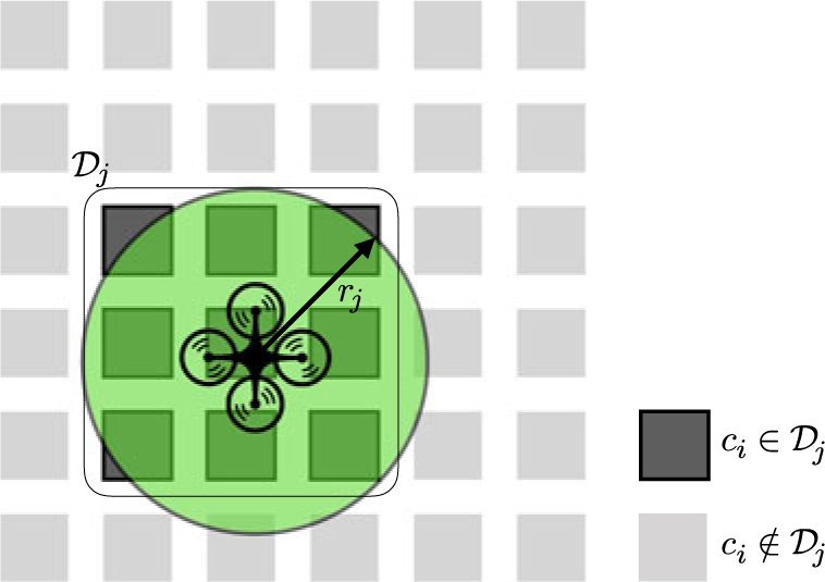
and Pj are the positions of cell i and agent j, respectively, and rj is the sensing radius of agent j. Figure 1 shows the sensing range of agent and set
 $\mathcal{D}_j$
.
Sensing range description.

In this study, the deterministic binary detection model is adopted for the agent detection model. Utilising the binary detection model, the age ai of a cell
 $c_i \in \mathcal{D}$
is instantly initialised to zero. Although various coverage control algorithms adopt probabilistic detection models and incorporate the probabilistic detection model into uncertainty dynamics for the sake of convenience in deriving the Jacobian, it can be argued that adopting the binary detection model is reasonable because sensors usually acquire information very rapidly relative to the uncertainty or agent dynamics.
2.2 Voronoi tessellation and Delaunay graph
The Voronoi region V = {V 1, ⋯, VM} can be generated with agent positions P = {P 1, ⋯, PM}. The Voronoi region can be defined as follows:
 $${V_j} = \{ s \in \Omega | d(s,{p_j}) \le d(s,{p_k}),\forall k \ne j\} $$
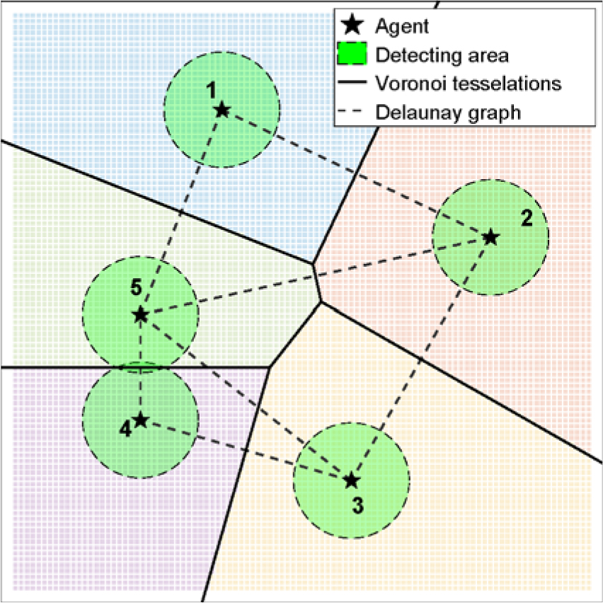
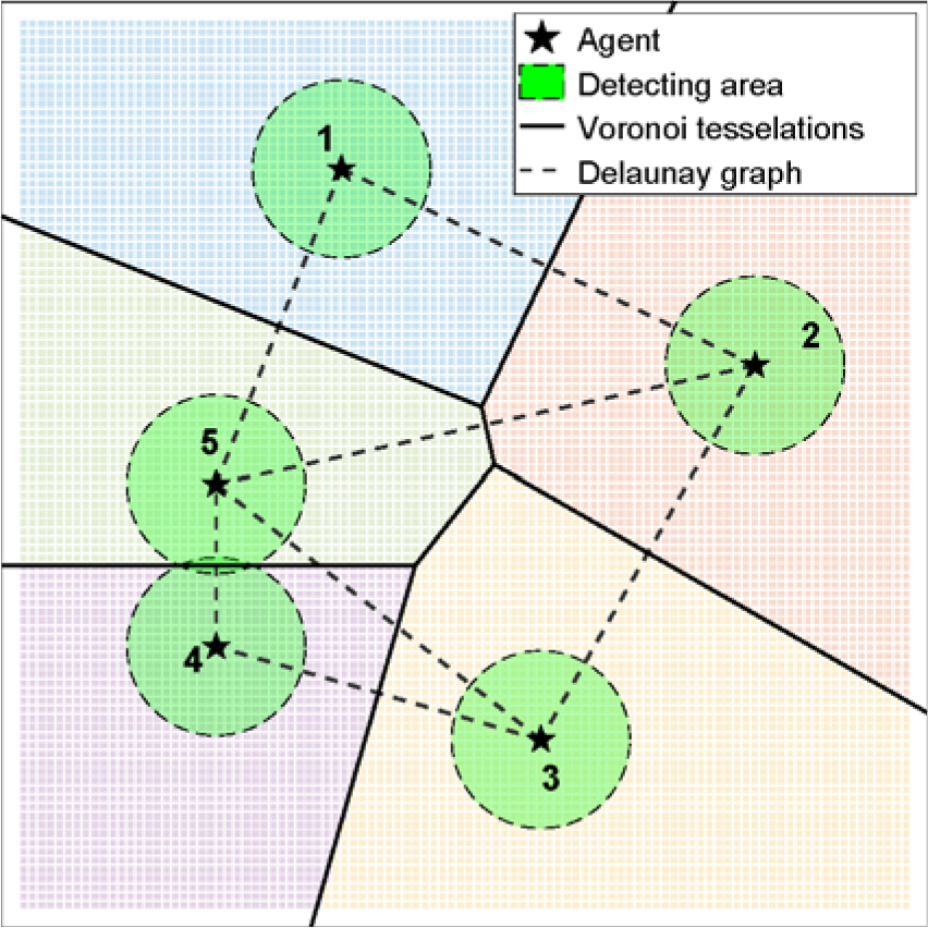
The Voronoi tessellation and Delaunay graph are common tools for designing distributed communication models of coverage control. Figure 2 shows the concept of the Voronoi tessellation and Delaunay graph. The Delaunay graph
 $\mathcal{G}=(\mathcal{V,E})$
is generated by connecting the agents with adjacent Voronoi regions. The vertices of the graph are allocated to each agent
 $\mathcal{V}=\{1,\cdots,M\}$
, and
 $\mathcal{E}\subset [\mathcal{V}\times\mathcal{V}] $
is the set of edges. When the agent pair (j, k) = (k, j) ∈ ℰ is the edge of the Delaunay graph
 $\mathcal{G}$
, agents j and k share their local information, including agent position Pj, Pk and predicted age vector
 $\mathcal{A}_j,\mathcal{A}_k$
, with each other.
Concept of the Voronoi diagram and Delaunay graph.
Each agent should know the information of Voronoi neighbours, which are the agents in the adjacent Voronoi region, to compute the Voronoi region of the agent itself. By means of the communication between Voronoi neighbours, a distributed coverage algorithm can be designed. The detailed algorithm about the communication between Voronoi neighbours can be found inReference Cortes, Martinez, Karatas and Bullo(18).
The Voronoi tessellation-based space dividing is motivated from the approaches in the distributed coverage control problem. Despite that the agents share their local information only with other agents in the adjacent Voronoi region, the agents can acquire up-to-date information of the entire space. Therefore, a distributed algorithm, in the aspect of information sharing between agents, can be designed using the Voronoi tessellation. It is beneficial to utilise the Voronoi tessellation not only because a distributed coverage algorithm can be designed but also the collision between agents can be avoided(Reference Palacios-Gasos and Sagüés14). The collision between agents in the monitoring space can be avoided because every agent moves toward a cell inside its Voronoi region, which is a convex set.
The neighbour set of agent j is defined as a set of connected agents denoted as
 $\mathcal{V}_j\subset\mathcal{V}$
. By means of local information sharing using the Delaunay graph, agent j can compute its Voronoi region Vj according to the distributed method. In addition, collision avoidance between the agents can be achieved based on the Voronoi tessellation because the agent j determines its action (target position, velocity direction) inside its own Voronoi region Vj.
Using the increasing dynamics of ai, each agent can predict the age ai of each cell ci and generate the predicted age vector
 $\mathcal{A}_j = [\hat{a}_1^{\,j}(t),\cdots,\hat{a}_N^{\,j}(t)]^T \in\mathbb{R}^N$
. Note that
 $\hat{a}_i^{\,j}$
is the predicted age of cell i by agent j. Because agent j can acquire only local information, the real age vector
 $\mathcal{A}=[a_1(t),\cdots,a_N(t)]^T$
may differ from the predicted age vector of the individual agent.
2.3 Performance function
The objective of persistent coverage control with the binary detection model is to continuously monitor the mission space without any blind spots or dead areas. That is, every cell in the mission space should be detected by agents in finite time. To evaluate the performance of the persistent coverage control, the following performance function is defined.
 $$C(t) = 1 - {{\sum\limits_{i = 1}^N \tanh (\rho {a_i}(t))} \over N}$$
where
 $\rho\in\mathbb{R}^+$
is a positive scaling constant. In this study, a hyperbolic tangent function is used in the numerator, but one can use any function f(ai(t)) that can bound the age as f(ai(t)) ∈ [0,1], ai(t) ≥ 0 to define the performance function in the range C(t) ∈ [0,1]. If there does not exist any agent available in the mission space, then the numerator in the performance function converges to N, and C becomes zero, indicating a zero coverage situation. By contrast, C = 1 implies the full coverage situation in which every cell in the mission space is detected by agents, i.e.
 $c_i\in\mathcal{D},\quad \forall i \in \{1,\cdots,N\}$
.
3.0 ANALYSIS FOR PERFORMANCE EVALUATION
In this section, the time behaviour of the performance function is analysed based on the predefined age dynamics and agent detection model defined in Section 2.0 to evaluate the performance. Performance evaluation means that the performance of given persistent coverage controller is evaluated based on the parameters and specifications of the monitoring space and the sensors (agents), which include the discretisation of the space, speed, and sensing radius of the agents.
The performance evaluation is conducted based on the following assumptions.
1 There is no loss of detecting area.
2 The number of detected cells per time is constant.
3 Every cell in the mission space is evenly detected.
The following analysis is performed based on the above assumptions. The first assumption states that the number of cells inside the sensing range is consistent. The second assumption is related to the modelling of the monitoring space and the sensor. The third assumption is adopted for the probabilistic analysis of the performance prediction. Based on the third assumption, it can be assumed that the statistical probability of detection for a cell is equivalent to all cells inside the mission space.
3.1 Steady-state analysis
It is assumed that the performance function converges to a steady-state value after the transition phase because the total increment of age is constant and there is a bound (limit) for the decrement amount. The total increment of ages over the mission space in time interval Δt can be written as
 $$\Delta {{\bf{a}}_ \uparrow } = (N - m)\Delta t$$
where m(< N) is the number of cells in
 $\mathcal{D}\subset\Omega$
, and m is assumed as constant in Assumption 1. In the steady state, the average age, as, of the cells being detected is constant. In addition, because the agents keep moving with constant speed μ and continuously detect new cells, the score decrement of ages can be represented as follows:
 $$\Delta {{\bf{a}}_ \downarrow } = - {a_s}{\mu _c}m\Delta t$$
where μc is the speed of the agent with respect to the number of cells, not to the distance. That is, μc is the number of cells passing by the agent moving with constant speed μ. Because the mission space is discretised into square cells, the number of cells passing by may not be consistent with respect to the velocity direction even though μ is constant. A hexagonal world representation may be helpful to alleviate this issue(Reference Quijano and Garrido19). To satisfy Assumption 2, μc should be constant. In this paper, μc is approximated as follows:
 $${\mu _c} \approx \mu \sqrt n $$
The sum of the age increment and decrement becomes zero in the steady state because the performance function is steady. The average age of the cells in the steady state as can be computed by the following simple equation:
 $$\Delta {{\bf{a}}_ \uparrow } + \Delta {{\bf{a}}_ \downarrow } = \Delta t((N - m) - {a_s}{\mu _c}m) \equiv 0$$
 $${a_s} = {1 \over {{\mu _c}}}\left( {{N \over m} - 1} \right)$$
Substituting as into the performance function gives the predicted steady-state performance Cs as
 \begin{equation}
C_{s} = 1-\frac{1}{N}\sum_{i\notin \mathcal{D}}\tanh\left( \rho a_{s} \right) \\ \quad \quad = 1-\left(1 - \frac{m}{N}\right)\tanh\left( \frac{\rho}{\mu_c}\left( \frac{N}{m}-1 \right) \right)
\end{equation}
3.2 Transient region analysis
For transient region analysis, a discretised span of time is considered. It is assumed that persistent coverage is guaranteed by monitoring the whole mission space Ω without leaving any blind spots. It is also assumed that the coverage algorithm can permit the agent to evenly detect all cells unless there exist some preferred cells. At each timestep, let p be the probability of an individual cell that has been detected during the past one second. That is,
 $i \in \mathcal{D}$
at least once during the arbitrary time interval [t, t + 1] when p = 1. Note that p is a constant based on Assumption 3. If the trial is conducted for every discretised time interval τ, then the probability of each trial is pτ.
The evaluated age of an individual cell
 $\bar{a}_i(t)=\mathbb{E}(a_i)$
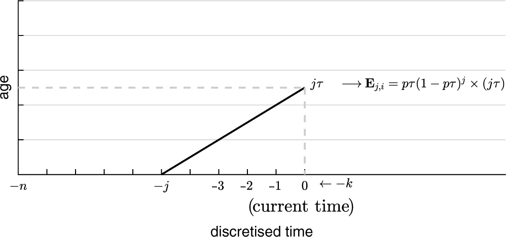
can be calculated by adding up the expected values of each trial. Figure 3 describes the discretised span of time and timesteps. The expected value
 $\mathbb{E}({a}_i)$
at time t is the summation of the expected values
 $\mathbb{E}_{k,i}$
at every
 $k\in\{0,1,\cdots\}$
timestep, which can be represented as
 $$\mathbb{E}({a}_i) = \lim_{n\rightarrow\infty}\sum_{k=0}^n \mathbb{E}_{k,i}$$
where
 \begin{array}{*{20}{c}}
{{\mathbb{E}_{0,i}}} \hfill & = \hfill & {p\tau \times 0} \hfill \\
{{\mathbb{E}_{1,i}}} \hfill & = \hfill & {p\tau (1 - p\tau ) \times \tau } \hfill \\
{{\mathbb{E}_{2,i}}{\rm{ }}} \hfill & = \hfill & {p\tau {{(1 - p\tau )}^2} \times 2\tau } \hfill \\
{} \hfill & \vdots \hfill & {} \hfill \\
{{\mathbb{E}_{n,i}}} \hfill & = \hfill & {p\tau {{(1 - p\tau )}^n} \times n\tau } \hfill \\
\end{array}
with
 $$\tau = t/n.$$
Span of time with timestep τ.

Note that
 $\mathbb{E}_{k,i}$
is the expected value when the cell
 $i\in\mathcal{D}$
at the k-th timestep and
 $i\notin\mathcal{D}$
until the current timestep, k = 0. Simplifying the geometric series and taking the extreme value
 $n\rightarrow\infty$
, we have
 \begin{array}{*{20}{c}}
{\bar a(t)} \hfill & = \hfill & {{\mathbb{E}}({a_i}) = \mathop {\lim }\limits_{n \to \infty } \sum\limits_{k = 0}^n p \tau {{(1 - p\tau )}^k}k\tau } \hfill \\
{} \hfill & = \hfill & {\mathop {\lim }\limits_{n \to \infty } \left[ {\frac{1}{p}\left( {1 - p\frac{t}{n}} \right)\left( {1 - {{\left( {1 - p\frac{t}{n}} \right)}^n}} \right) - {{\left( {1 - p\frac{t}{n}} \right)}^{n + 1}}} \right]} \hfill \\
{} \hfill & = \hfill & {\frac{1}{p} - {e^{ - pt}}\left( {\frac{1}{p} + t} \right)} \hfill \\
\end{array}
Note that the subscript (⋅)
i is omitted for the evaluated age
 $\bar{a}(t)$
because it is assumed that the average value of age is considered not a certain age of the cell ci. Now, p and
 $\bar{a}_i(t)$
can be obtained using the steady-state value as as
 $${a_s} = \mathop {\lim }\limits_{t \to \infty } \bar a(t) = {1 \over p}$$
where
 $$p = {{{\mu _c}m} \over {N - m}}$$
 $$\bar a(t) = {1 \over {{\mu _c}}}\left( {{N \over m} - 1} \right) - {e^{{\mu _c}mt/(N - m)}}\left( {{1 \over {{\mu _c}}}\left( {{N \over m} - 1} \right) + t} \right)$$
Substituting
 $\bar{a}_i(t)$
into the performance function yields the predicted performance
 $\bar{C}(t)$
as
 $$\bar C(t) = 1 - \left( {1 - {m \over N}} \right)\tanh \left( {\rho \bar a(t)} \right)$$
Note that the predicted age and predicted performance are calculated based on the assumption that m is constant. The overlapping of detection ranges between the agents as well as the loss of detection ranges when detecting the boundary of the mission space is not considered in this analysis. That is,
 $\mathcal{D}_j(t) \cap \mathcal{D}_k(t) = \emptyset$
and
 $\mathcal{D}_j(t) \subset \Omega,\forall (j,k)\in\{1,\cdots,N\},\forall t$
. The predicted mean age and predicted performance are calculated as functions of agent speed, detection range combined with the number of agents, and the number of cells in the mission space.
4.0 PERSISTENT COVERAGE CONTROL APPROACH
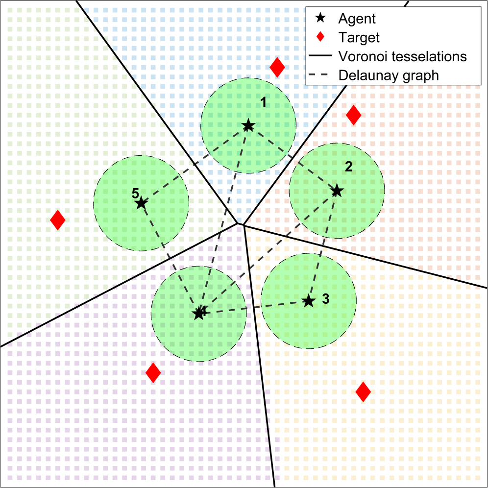
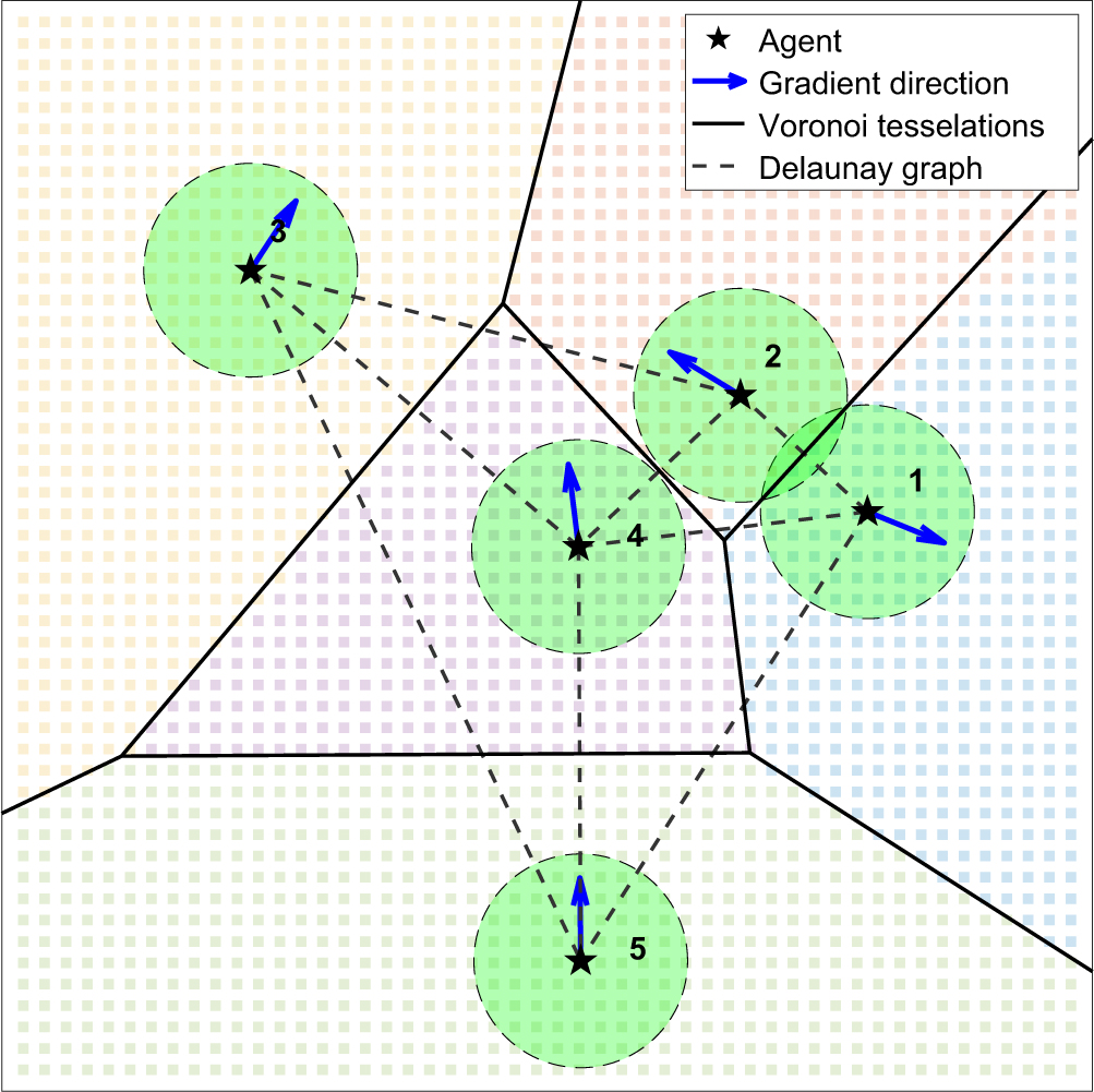
In this study, two different persistent coverage control algorithms are considered to compare the performance of the algorithms using the predicted performance. Snapshots generated by conducting two designed persistent coverage control algorithms are shown in Figs. 4 and 5.
Snapshot of the target-based approach.

Snapshot of the gradient-based approach.

Note that the optimal persistent coverage control problem is an NP-hard problem, which is difficult to solve and time consuming. The target-based approach is one possible and easy heuristics to deal with this problem.
Meanwhile, the reactive approach is one of widely used methods in the coverage control problems. In the coverage control problem, the reactive controller calculates the gradient of a given weight function defined in the monitoring space. There is a difference between the coverage control problem and the persistent coverage control problem; that is, the weight function to calculate the gradient changes continuously. Therefore, the reactive controller in the persistent coverage problem makes the agent move persistently and does not converge to a particular position.
Distributed persistent coverage control algorithms are designed so that the individual agent uses only local information to achieve persistent coverage of the entire mission space. The local information for agent j consists of
 $(P_j, \mathcal{A}_j)$
, and
 $(P_k, \mathcal{A}_k)$
of neighbouring agents
 $k\in\mathcal{V}_j$
. The information update rule for agent j is as follows:
 $$\hat a_i^{{\kern 1pt} j} \leftarrow \min \left( {\hat a_i^{{\kern 1pt} j},\hat a_i^k} \right),\quad \forall k \in {{\cal V}_j},\quad \forall i \in \{ 1, \cdots ,N\} $$
The minimum value of the predicted age is the most correct because the age is monotonically increasing; therefore, the cell with a smaller age represents the cell detected by the agent more recently.
4.1 Target-based approach
The target-based control approach guides agent j to a certain target cell, tj. The cell with the maximum age inside the Voronoi region is determined as a target cell, and the agent is guided to position Tj of the target cell tj.
 $${t_j} = \mathop {{\rm{argmax}}}\limits_{{c_i} \in {V_j}} \left( {\hat a_i^j} \right),\quad \hat a_i^j \in {A_j}$$
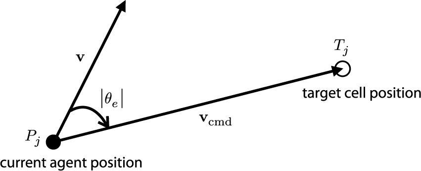
Figure 6 shows the geometry between Pj and Tj. The angular error θe is defined as follows:
 $${\theta _e} = |{\theta _e}|e$$
where
 $$|{\theta _e}| = \mathop {\cos }\nolimits^{ - 1} \left( {{\bf{v}} \cdot {{\bf{v}}_{}}cmd} \right)$$
 $$e = - {\rm{sign}}({{\bf{v}}_n}(3))$$
 $$\mathbf{v} = \left[\begin{array}{@{}c@{}}\mu \cos\theta_j\\\mu\sin\theta_j\\0\end{array}\right]\!,\quad
\mathbf{v}_\textrm{cmd} = \left[\begin{array}{c}T_j(1)-P_j(1)\\T_j(2)-P_j(2)\\0\end{array}\right]\!,\quad
\mathbf{v}_n = \mathbf{v}\times\mathbf{v}_{cmd}$$
Geometry between the agent position and target position.

Now, the error dynamic can be designed as follows:
 $${\dot \theta _e} = {d \over {dt}}\left( {{\theta _{}}_{{\rm{cmd}}} - {\theta _j}} \right) = - {\dot \theta _j} = - k{\theta _e}$$
where k is a positive scalar gain. The target-based control input uj that makes the error exponentially converge to zero can be designed as follows:
 $$u_i^0 = {\dot \theta _j} = k|{\theta _e}|e$$
Considering the maximum limit of the control input, we have
 $$u_i = \left\{\begin{array}{@{}cl@{}} u_\textrm{lim} & \textrm{if } u_i^0\ge u_\textrm{lim}\\\\ u_i^0 & \textrm{Otherwise}\\\\ -u_\textrm{lim} & \textrm{if } u_i^0\le -u_\textrm{lim} \end{array}\right.$$
4.2 Reactive approach
The reactive control approach guides the agent to the centre of mass direction of the age distribution in the mission space. The individual agent j computes the direction using the evaluated age vector  $\mathcal{A}_j$, which is local information. The heading command is computed based on the age of the cells detected by the agent. Because the age of the detected cells is initialised to zero, the agent computes the direction before initialising the predicted age of the newly detected cells. The center of mass Cj is computed as follows:
 $$\quad {C_j} = {{{L_j}} \over {{M_j}}} \in \Omega $$
where Mj and Lj are mass and first moment of the detection range
 $\mathcal{D}_j$
.
 $${M_j} = \int_{s \in {{\cal D}_j}} \hat a_i^{{\kern 1pt} j}ds,\quad {L_j} = \int_{s \in {{\cal D}_j}} \left( {s \cdot \hat a_i^{{\kern 1pt} j}} \right)ds$$
The same guidance law is applied to the reactive control approach, but the command vector vcmd is defined as follows:
 $$\mathbf{v}_\textrm{cmd} = \left[\begin{array}{c}
C_j(1)-P_j(1)\\C_j(2)-P_j(2)\\0\end{array}\right]$$
5.0 NUMERICAL SIMULATION
5.1 Evaluation and simulation
A numerical simulation is performed to demonstrate the usefulness of the proposed method. The difference between the simulation result and the evaluated value is the result of the assumptions, which differ from those in the simulation situation. The first factor is the approximation of μ c in Equation (11), which is related to Assumption 2. The actual μ c varies along the velocity direction of the agent because the mission space is discretised into square cells. For instance, μ c = μn when the velocity direction is [0, 1] or [1, 0]. Because this may be a low estimate of the real velocity with respect to the cells, the predicted performance of the coverage is lower than that of the simulation result. Note that the square discretisation of the mission space results in directional symmetry in four directions (0,π / 2,π and 3π /2 directions). Hexagonal discretisation(Reference Quijano and Garrido19) of the mission space would bring about six directional symmetry and may lower the approximation discrepancy of μ c.
The second factor is a redundant detection, which is related to Assumption 3. Redundant detection occurs when a certain cell is detected again before its age increases to the predicted mean age due to the physical location of the cell and agent. That is, cells with low age may be on the path of the agent moving to its target cell, and therefore it will be detected redundantly. Redundant detection may lower the performance of coverage compared to the evaluated performance.
The third factor is the assumption of constant m. Detection ranges may overlap between agents. In addition, loss of detection range would occur when the agent is close to the boundary of the mission space. This factor is related to Assumption 1.
In this study, four simulation cases are considered. Simulations of Case A and Case B are conducted to demonstrate the properties of the evaluation model using proper simulation parameter settings. Different numbers of agents and agent speeds are considered in Case A and Case B, respectively. The steady-state evaluation and simulation results are compared with respect to each other. Simulations of Case C and Case D are performed to illustrate how the evaluation performance is affected by discrepancies between the assumptions and actual simulation situations. The sensing range (sensing radius of the agent) and space discretisation level n are varied in Case C and Case D, respectively. The values of m and μc are computed during the mission, and the average values are compared with the approximated value used in the evaluation model.
5.2 Case A. Number of agents
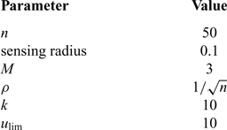
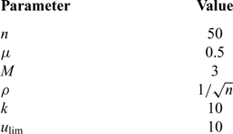
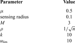
In this section, a numerical simulation is performed to demonstrate the performance of the designed persistent coverage controllers. The performance of the persistent coverage controllers is compared with the predicted performance described in Section 3.0. The simulation conditions are summarised in Table 1.
Simulation settings of Case A (agent number variation)

Adequate simulation parameters are set empirically. The constant m is computed from the relative extent of the sensing range (area) with respect to that of the mission space Ω.
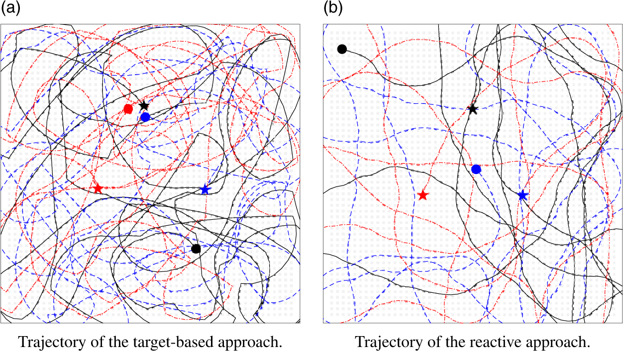
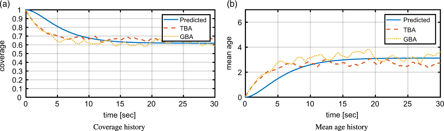
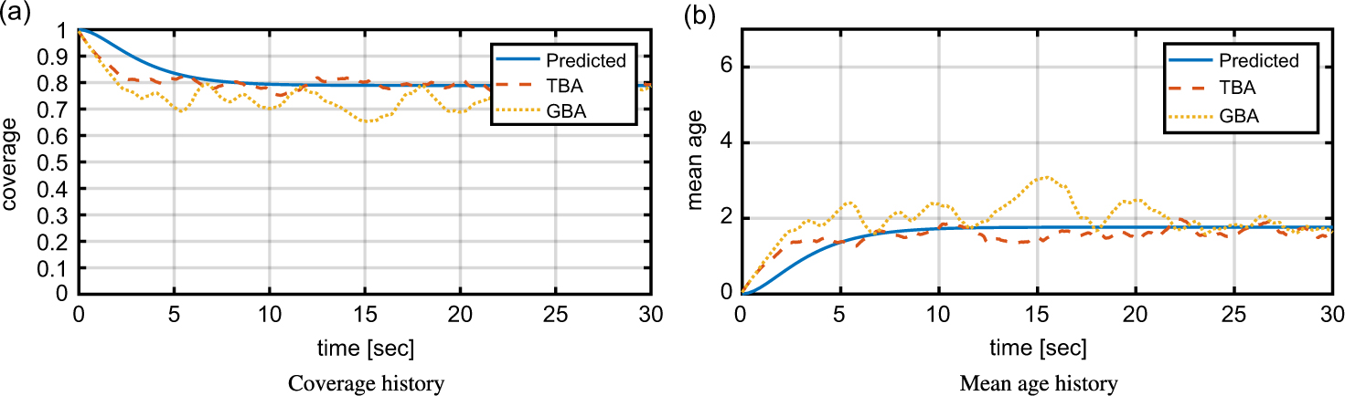
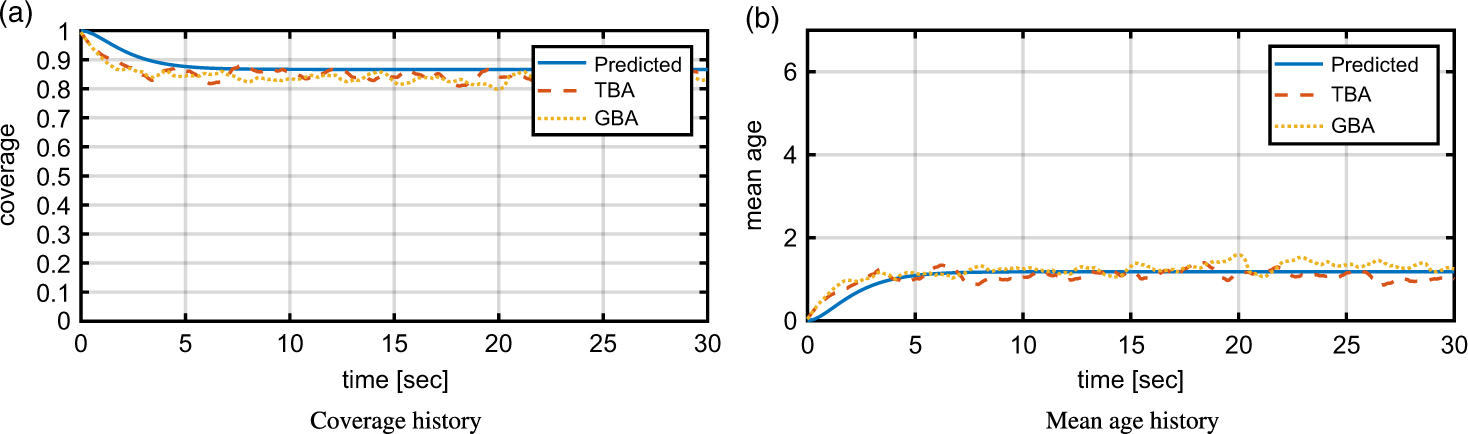
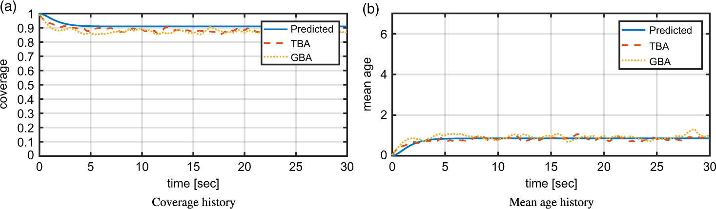
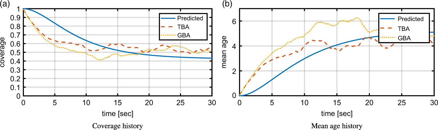
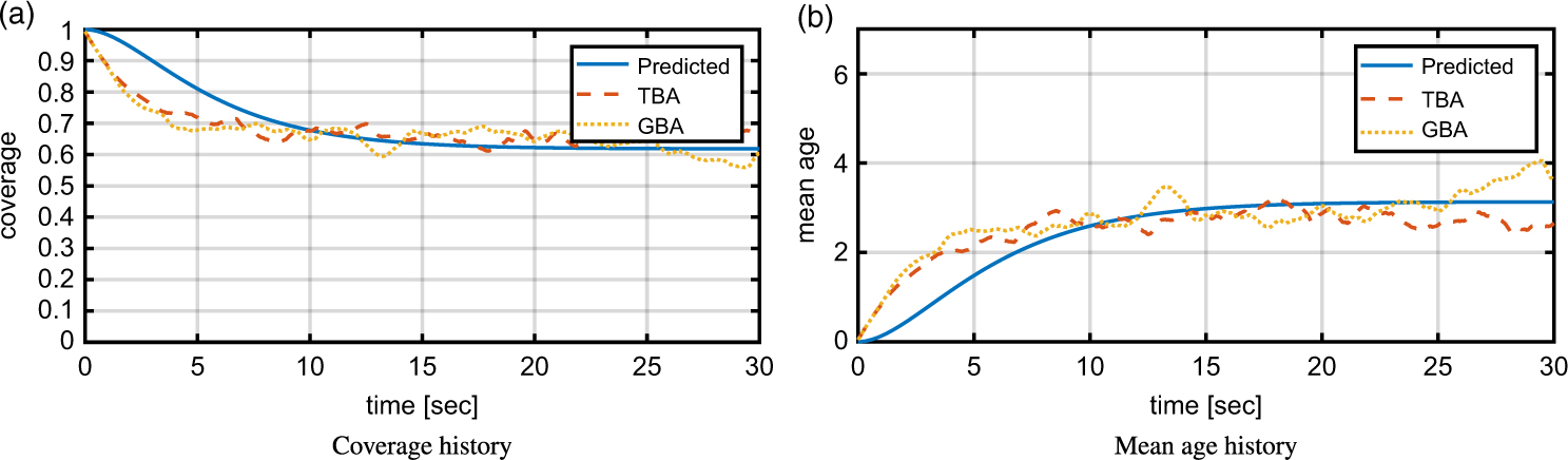
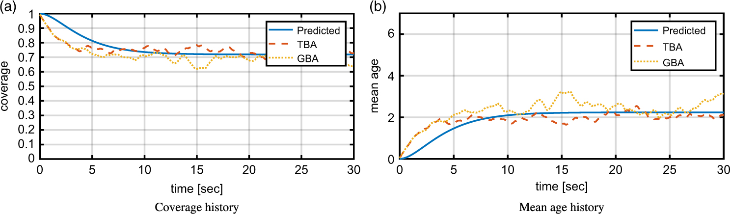
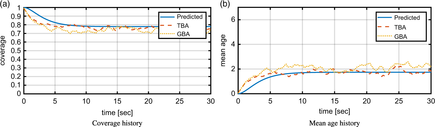
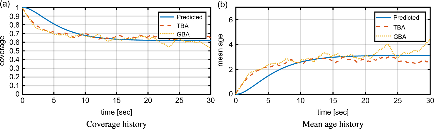
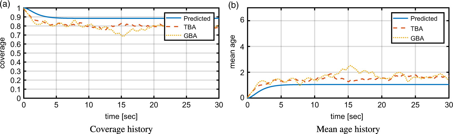
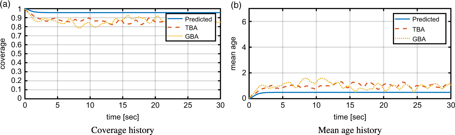
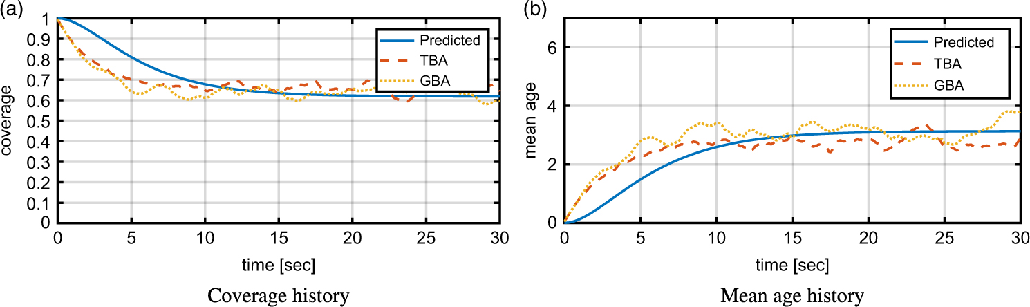
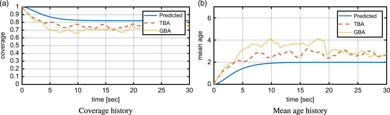
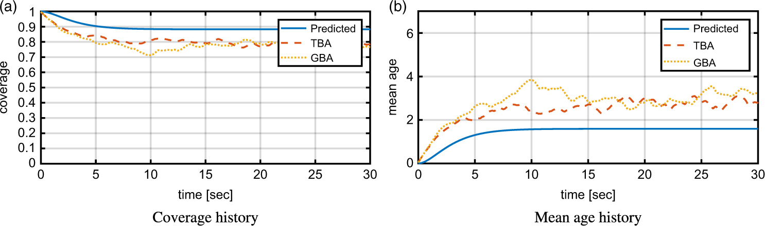
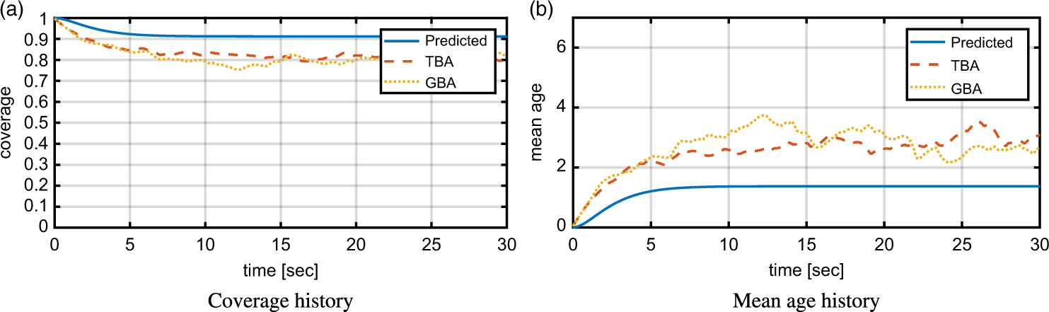
Figure 7 shows the trajectories of the agents for the target-based approach (TBA) and gradient-based approach (GBA). The pentagrams and filled circles are the initial positions and final positions of the agents, respectively. The lines in the figure show the paths of the agents. Figures 8 to 11 are the simulation results and predicted values for various numbers of agents. Both the target-based control approach and the reactive control approach show convergence to the steady-state value of mean age with some fluctuations. The predicted mean age and predicted coverage, denoted as a solid line, show decent evaluation of the mean age and coverage values.
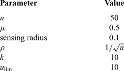
Simulation settings of Case B (agent speed variation)

Trajectory of agents.

Coverage history and mean age history (three agents).

Coverage history and mean age history (five agents).

Coverage history and mean age history (seven agents).

Coverage history and mean age history (nine agents).

The initial age of every cell is zero, and therefore the mean age and coverage start from 0 and 1, respectively. Note that as the number of agents increases, the transient phase is short, and the evaluated age and performance coverage converge to the steady-state values quickly. It is natural that the steady-state mean age is lower as the number of agents increases, and the performance of coverage increases as well.
5.3 Case B. Speed of agents
The speed of the agent is also a major factor affecting steady-state performance. The simulation settings are summarised in Table 2. Figures 12 to 15 show the coverage performance and mean age history as μ increases. A faster agent speed gives faster convergence to the steady-state performance and higher steady-state performance value. The evaluated performance in the steady state increases and the transient phase becomes shorter as the speed of the agent increases. These results are due to the denominator μ c and exponential term in Equation (20), respectively.
Coverage history and mean age history (μ = 0.3).

Coverage history and mean age history (μ = 0.5).

Coverage history and mean age history (μ = 0.7).

Coverage history and mean age history (μ = 0.9).

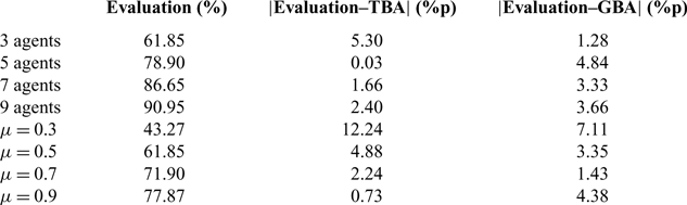
The simulation results for Case A and Case B are summarised in Table 3. The Evaluation column in the table represents the steady-state coverage performance as a percentage. The other columns represent the difference between the evaluated value and the simulation results of TBA and GBA as percentages. The differences are less than 10%p for every simulation conducted except for one case. Note that the same simulation conditions are considered for the first row (Case A) and sixth row (Case B), but the numerical results are slightly different due to the random initial values of each agent’s predicted age vector.
Steady-state evaluation performance in Cases A and B

5.4 Case C. Sensing range
Simulations of Case C and Case D are conducted to illustrate the effectiveness of the discrepancy between the assumptions and the actual simulation situations. In Case C, the effect of the sensing radius of the agent is considered. A larger relative size of the sensing range with respect to the size of the mission space may affect the simulation performance because it may incur more frequent overlapping of the sensing range between agents and loss of detection range near the mission space boundary. The simulation settings are summarised in Table 4.
Simulation settings of Case C. (sensing radius variation)

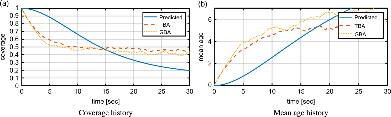
Agents with a larger sensing range can detect more cells. However, redundant detections are induced more frequently, and the assumption of constant m is violated more often during the simulation because of the overlapping and loss of detection ranges between agents. Figures 16 to 19 show the coverage and mean age history for various sensing radii.
Coverage history and mean age history (sensing radius = 0.05).

Coverage history and mean age history (sensing radius = 0.10).

Coverage history and mean age history (sensing radius = 0.15).

Coverage history and mean age history (sensing radius = 0.20).

5.5 Case D. Level of space discretisation
In the simulation of Case D, different discretisation levels n are considered. The simulation settings are summarised in Table 5. Because the discretised space is adopted to construct an age model approximating the real continuous space, it is natural to expect that a dense discretisation would result in a more realistic evaluation than sparse discretisation.
Simulation settings of Case D (space discretisation level variation)

Figures 20 to 23 show the coverage history and mean age history to compare the evaluated performance and simulation results with respect to various discretisation levels, n. The trend of the difference between the evaluated performance and the simulation result is analogous to that of Case C.
Coverage history and mean age history (n = 50).

Coverage history and mean age history (n = 100).

Coverage history and mean age history (n = 150).

Coverage history and mean age history (n = 200).

5.6 Comparative analysis
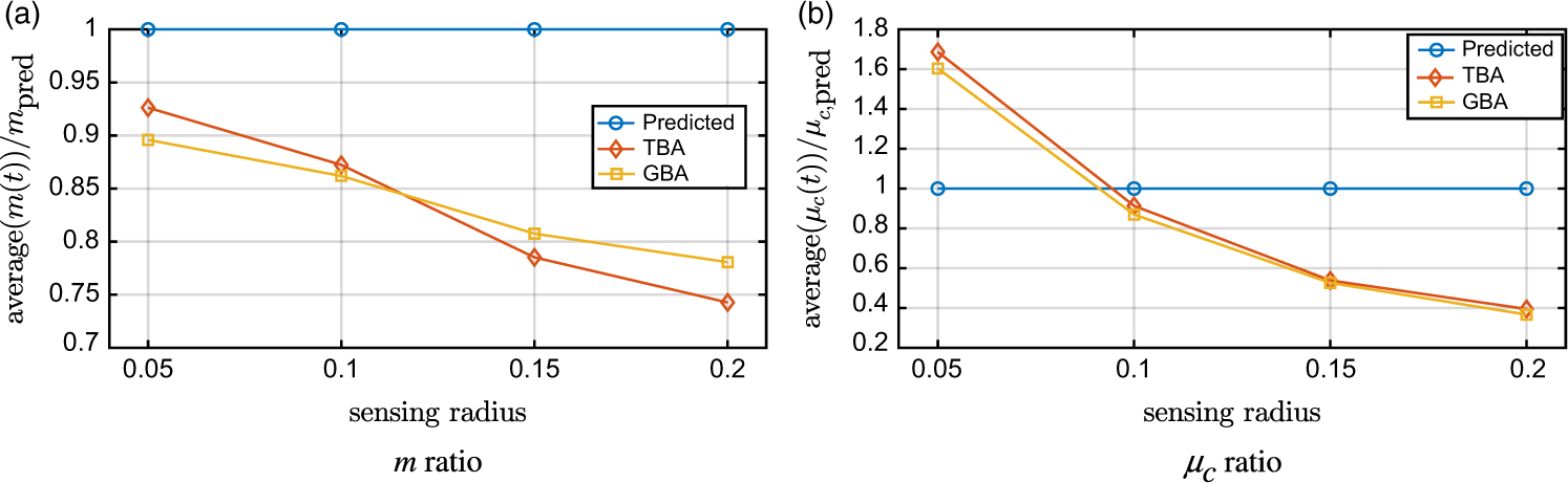
Figure 24 shows the differences between the evaluation and simulation. The constant m and μc assumptions are violated to different extents. In Fig. 24(a), the average m is divided by m pred, which is used in the evaluation. In Fig. 24(b), the average μc is divided by μ c,pred. Because the overlapping and loss of sensing range increase along with the sensing radius, the relative ratios of the average m and average μc (in the simulation) to the assumed m pred and
 $\mu_{c,\textrm{pred}}(=\mu \sqrt{n})$
decrease. As a result, whereas the steady-state evaluation of coverage is lower than the simulation result in Fig. 16, it becomes higher than the simulation result as the sensing radius increases (Figs 17 to 19).
Difference between the evaluation and simulation with respect to the sensing radius.

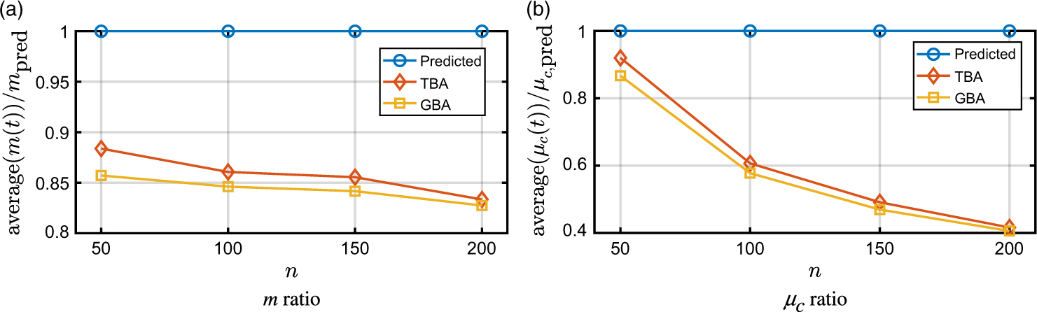
Fig. 25 shows the differences between the evaluation and simulation situation with respect to n. As shown in Fig. 25(a), the discretisation level does not have much of an effect on the change in m. However, as shown in Fig. 25(b), making the discretisation level dense has an adverse effect upon the μc assumption. That is, the approximation in Equation (11) becomes invalid. As a result, the steady-state coverage performance is overestimated in dense discretisation as shown in Fig. 23. Note that the basic reason for the overestimation is the inadequate μc approximation, rather than the dense discretisation level.
Difference between evaluation and simulation with respect to discretisation level.

6.0 CONCLUSION
The persistent coverage control problem was modelled with the uncertainty model based on age and the binary deterministic detection model of monitoring agents. Two controllers, the target-based controller and reactive controller, were designed using local information based on the Voronoi diagram and information sharing via the Delaunay graph. The performance of the general persistent coverage control algorithm was evaluated and calculated as a function of the mission space parameters and the speed of the monitoring agent. The performance evaluated by the proposed method was compared with the performance of two different persistent coverage controllers.
Differences were observed between the evaluated performance and the simulation results. The differences in the evaluation are induced by the assumptions, which differ from the actual simulation situations, i.e. the constant speed approximation, redundant detection, and constant number of cells in the sensing region assumption. The factors responsible for the differences were computed by numerical simulation, and the interrelations between the factors and mission space-describing parameters were discussed. The mission space-describing parameters are the relative size of the sensing range with respect to the mission space and the discretisation level of the mission space. Based on this knowledge, one may select adequate assumptions and approximations of parameters for accurate performance evaluation. The evaluated mean age and performance function values provide useful and meaningful evaluation of the coverage control performance by setting proper simulation parameters, including the discretisation level.