


A key question in political economics is how institutions shape political behavior. In democracies, elections forge a critical link in the principal-agent chain between voters and politicians. When voters are unhappy with politicians’ or parties’ actions in office, elections give them the crucial opportunity to “throw the rascals out” (Barro Reference Barro1973; Ferejohn Reference Ferejohn1986). Nevertheless, the power of the vote is limited. Many politically influential positions—such as party leaders, chairs of legislative committees, or even prime ministers—are never subject to a popular vote. Even when direct elections are held, parties usually present voters with a restricted set of candidates. How political parties select individuals for appointments or candidates for elections is often labeled the “black box of party politics” or the “secret garden” of party nominations (Gallagher and Marsh Reference Gallagher and Marsh1988).
In this article, we analyze the interplay between the electoral system and parties’ internal organization. We develop and test an entirely new hypothesis: thatthe distribution of votes across political candidates in the general election guides internal party decisions on promotions to influential appointments. If true, this hypothesis implies that citizens’ votes matter beyond their direct impact on electoral outcomes. If election results indeed guide party promotions, the information that parties obtain should be considered when evaluating and comparing different electoral systems, in particular when it comes to accountability.
Proportional election systems with open or semi-open lists allow voters not only to cast ballots for parties but also to cast preference votes for individual candidates from their preferred party. We analyze how these preference votes affect the nomination and promotion behavior of political parties. Our main analysis focuses on Swedish municipalities, which have used semi-open lists since 1998. We also consider a very different electoral context: open lists in Brazilian municipal elections.
Why should parties use preference-vote tallies to guide their internal organization? First, preference votes give parties information about the popularity and electability of individual candidates (Crisp et al. Reference Crisp, Olivella, Malecki and Sher2013). This information could be valuable for office-maximizing parties if popular politicians have better chances of winning elections, either as individual candidates or as key actors of party groups. Second, using preference votes makes the nomination and promotion processes more transparent, similar to primary elections in majoritarian election systems (Kemahlioglu, Weitz-Shapiro, and Hirano Reference Kemahlioglu, Weitz-Shapiro and Hirano2009; Ware Reference Ware2002). More transparency could help reduce the risk of strong intraparty conflict (or limit the negative consequences of such conflict). It may also benefit parties at the ballot box if voters reward parties that select candidates objectively.
An empirical analysis of party responses to preference-vote tallies requires careful consideration of endogeneity problems. A positive correlation between preference votes and subsequent political promotions need not reflect a causal effect of preference votes. If more able politicians move up the power ladder and at the same time gain more preference votes, we might mistakenly attribute their career moves to preference-vote support when the true (omitted) reason is politician quality. Because drivers of votes and career advancement are likely unobserved by the researcher, control variables may be insufficient to tackle such omitted-variable bias. In sum, we need a better method than standard regression analysis to estimate the causal effect of preference votes on promotions.
In this article, we apply a regression discontinuity design (RDD) around the threshold for winning the most preference votes within the party group.Footnote 1 If the top-two preference-vote earners have similar vote tallies, they are likely similar in terms of both observed and unobserved characteristics. In this quasi-experimental setting, we can consider very close races as approximately random draws of winners and losers. A battery of robustness checks confirms that this is indeed the case.
Comparing close winners and losers, we show that the causal impact of winning the most preference votes raises the probability of political career advancement. We label this the “primary effect” (of the preference votes). In our main analysis of Sweden, we find that if a politician wins the most preference votes in an election, he or she is about 60% more likely to be at the top of the party ballot in the next election. We find even larger primary effects when analyzing appointments to specific positions of power, most importantly the chair of the municipal council board (the equivalent of mayor). Winning the preference-vote primary more than doubles the probability of appointment to this position.
Moreover, we also uncover a primary effect—of about the same relative size—on the behavior of local parties in Brazil. The politicians who obtain the most votes in a city-council election substantially raise their probability of becoming the party's unique candidate in the election to the most powerful local political position in Brazil, namely that of mayor. The fact that we find similar results in Sweden's semi-open-list system and in Brazil's open-list system strongly suggests that the primary effect is a general political phenomenon that extends across electoral systems and levels of economic and political development. The preliminary results in Meriläinen and Tukiainen (Reference Meriläinen and Tukiainen2015), which indicate that a primary effect is also present in Finland's open-list system, point in the same direction.
An extended analysis of the Swedish case explores whether individual characteristics of the winners of the preference vote matter for parties’ promotion behavior. Distinguishing preference-vote winners by list rank shows that the primary effect is only important for politicians who have already reached a high enough position in the party hierarchy. This finding suggests that voter support complements, but does not substitute for, party support. Considering the competence of winners and runners-up reveals a primary effect only when the two candidates have similar competence levels. This finding suggests that parties learn useful information about candidate popularity from preference votes and use this information in awarding promotion among otherwise comparable candidates.
We also consider heterogeneity in party behavior depending on the political context: external competition (i.e., competition among political parties) and internal competition (i.e., competition within a party depending on the number of top positions it can appoint). Both types of competition seem to contribute to a closer adherence to preference votes in party promotions. Interestingly, preference votes trigger leader changes even in local political monopolies, in which the governing party does not need to cater to voters to win the election. This finding indicates that internal party motives, such as reducing fractional fighting, may be important in explaining the rationale behind the primary effect.
This article is structured as follows. In the theory section we develop the case for why preference votes can have a primary effect and provide three testable predictions. In the following sections we describe a strategy for estimating the causal primary effect and then present our main case, Swedish municipalities. The results from our main case are divided into two parts: The first presents the main results that strongly support the existence of a primary effect, whereas the second part presents the results for our additional predictions on how the primary effect hinges on candidate characteristics and political contexts. After this we describe our data and results for Brazil. Auxiliary results and robustness checks are available in the Online Appendix.
Theoretical Discussion and Empirical Predictions
A wealth of research has outlined how the relationship between politicians and parties reflects three main aspects of electoral institutions: the electoral formula, district magnitude, and candidate-selection rules. In this paper we consider only the latter two, under the same electoral formula, namely proportional representation (PR). We can think about these institutions along a single dimension from the most party centered to the most candidate centered. The most party-centered PR systems have closed lists and large districts. Individual candidates have little accountability in such systems, because their reelection hinges on support from the party leadership rather than from voters (for a review of the relevant literature, see Shugart Reference Shugart2013). The least party-centered PR systems have open lists, in which voters decide who is elected by ranking their preferences. This system is criticized for leading to low party cohesion, because the parties have weaker control over who is elected from their ballots.
A common reform to strengthen candidate accountability to voters in closed-list systems is to introduce semi-open lists. These allow voters to cast preference votes among individual candidates on a preordered list, but candidates are only elected based on preference votes if they exceed a certain threshold. However, this type of reform has generally not been well received. Critics point out that voters predominantly support candidates at the top of the list, which makes the number of preference votes largely inconsequential for who gets elected. Many researchers thus conclude that semi-open lists are “in practice, very similar to closed-list PR systems” (Hix Reference Hix2004, p. 197); see also Andeweg Reference Andeweg, Gallagher and Mitchell2005; De Winter Reference De Winter, Gallagher and Mitchell2005; Farrell Reference Farrell2001; Mueller Reference Mueller, Gallagher and Mitchell2005).
This classification of electoral systems pivots around the consequences of who gets elected. Although certainly interesting and important, who gets elected is only one dimension of political power. Parties are hierarchical organizations, in which politicians in top positions (compared to those in less powerful positions) have a greater say on party platforms (Harmel et al. Reference Harmel, Heo, Tan and Janda1995), act as party spokespersons, draw votes (Bittner Reference Bittner2011; Stewart and Clarke Reference Stewart and Clarke1992), participate in coalition formation (Laver and Schofield Reference Laver and Schofield1990), and heavily influence decisions on recruitment and promotion (Bille Reference Bille2001; Dowding and Dumont Reference Dowding, Dumont, Dowding and Dumont2009). Political officeholders are sometimes directly elected by the voters, but more often they are not. Parties appoint both executives—such as prime ministers or mayors—and mid-level posts like committee chairs. They also select candidates for higher offices. How specific institutions affect these promotion decisions is a crucial but previously neglected dimension in studies of electoral systems. Specifically, we argue that the presence of preference votes will affect parties’ promotion decisions. We next present our arguments for why this is the case.
Previous research has argued that parties in party-centered list systems have strong motives to place popular persons—for example, those with good (local) reputations (Shugart, Valdini, and Suominen Reference Shugart, Ellis Valdini and Suominen2005; Tavits Reference Tavits2010)—high on their electoral lists (Crisp et al. Reference Crisp, Olivella, Malecki and Sher2013) so as to maximize their vote share. We argue that the same claim should hold for promotions and appointments to top positions. Because there are few opinion polls on individual politicians in list-based PR systems, parties must typically rely on indirect measures of popularity, such as their own perceptions of candidate competence and loyalty. However, in open or semi-open lists the number of preference votes gathered by each politician on the party ballot provides a direct popularity measure. In fact, voters may be better than parties at picking electorally viable candidates (Carey and Polga-Hecimovich Reference Carey and Polga-Hecimovich2006). Thus, by promoting their most popular politicians, parties can raise their chances of electoral success (authors' own interviews). Parties may promote candidates for offices up for direct election (such as elected mayors) or for higher offices appointed by the party (like appointed mayors).
Using preference votes in promotion and nomination decisions could not only improve a party's electoral fortunes by improving the selection process but it could also have a direct, and independent, impact on the party's electoral performance. A promotion process that incentivizes individual politicians to go out and seek votes is clearly aligned with the party's overall goal of winning elections and could also be expected to raise the overall vote count. Moreover, because voters care about policy, they have motives to influence the allocation of power within parties. In other words, parties can attract voters by letting them select between politicians with different policy preferences. These benefits are supported by earlier research. Thirty years ago, Wildgen (Reference Wildgen1985) discussed the electoral strength of the Italian Christian Democratic party in the post–World War II era. This strength, he argued, stemmed from strong competition for preference votes between the party's politicians, a feature that attracted more voters to the party. We can also look to more recent work. For example, Blumenau et al. (Reference Blumenau, Eggers, Hangartner and Hix2014) use a laboratory setting to show that parties with clear ideological differences between their candidates benefit electorally when preference voting is introduced.
The effect of a party's giving voters nomination power through preference votes in PR electoral systems is in many ways similar to giving them nomination power through primary elections in majoritarian election systems. The introduction of primaries has received wide scholarly attention and could thus provide important insights for our argument. This literature suggests that the key motive for introducing primaries is to replace “smoke-filled rooms” with a more transparent nomination procedure, which is is expected to yield two types of benefits. First, it combats internal party divisions, as shown in the U.S. South (Key Reference Key1949) and Latin America (Hortala-Vallve and Mueller Reference Hortala-Vallve and Mueller2012; Kemahlioglu, Weitz-Shapiro, and Hirano Reference Kemahlioglu, Weitz-Shapiro and Hirano2009; Serra Reference Serra2006). The second benefit is that the party will attract more votes if voters have a preference for more transparent nomination procedures such as voluntary primaries (Carey and Polga-Hecimovich Reference Carey and Polga-Hecimovich2006) or legally introduced primaries (Ware Reference Ware2002).
Finally, if parties use preference votes for promotion, they need to use a decision rule. A simple and objective rule, which could also have symbolic importance, is that the top appointment should be given to the most popular candidate (i.e., the one with the most preference votes). This idea corresponds to anecdotal evidence of objections against failures to follow this rule. Katz (Reference Katz1980, p. 74) observes the case of Italy's now abandoned open-list system, noting that it was “the universal expectation” that the capolista (the top name on the ballot) would win the most preference votes. If he or she did not, this was interpreted as “a serious misjudgment by the party leadership.” This argument supports our idea that preference votes provide a reading on candidate popularity. Similar evidence can be drawn from Swedish newspaper coverage of party appointments. It is not uncommon that news articles highlight the preferential vote “winner” and charge parties with weak accountability and ignorance of the popular if this candidate is not given the party's top appointment.Footnote 2
In sum, political parties may have a strong incentive to base promotions on the distribution of preference votes among their politicians. This approach may help parties promote the most popular candidates and provide a direct incentive to vote for the party. It may also help parties avoid internal conflict and appeal to voters via objective criteria for candidate promotion. In this promotion decision, winning the most votes in a party group should be of particular importance. Based on this discussion, we make the following prediction:
P1 – The Primary Effect
The individual who obtains the most preference votes in a party group has a greater probability of future political promotion.
We note in passing that if some voters believe that parties use preference votes in the way we claim, then casting their preference vote then becomes an intricate problem for voters who take the behavior of other voters into account, rather than just vote sincerely for the candidate they like the best. This is an instance of a general issue explored in the theoretical voting literature, namely that a certain outcome or poll also has “downstream” effects (Meirowitz and Shotts Reference Meirowitz and Shotts2009; Piketty Reference Piketty2000; Razin Reference Razin2003). If a single promotion—for example, to party leader—is at stake, strategic voters should realize that supporting their favorite candidate may waste their preference vote if few other voters support this candidate. As in the work on strategic voting in first-past-the-post elections (e.g., Cox Reference Cox1987), Duvergerian logic implies that preference votes should become concentrated on a few candidates.
The Primary Effect is our main hypothesis and the main focus of our empirical work. We also develop two additional (sets of) conditional predictions to better understand the behavior of parties. Specifically, we explore how the primary effect might differ depending on political contexts and individual candidate characteristics.
If parties use preference votes to obtain information for appointments to positions of power, then semi-open or open lists can clearly strengthen the political accountability of individual politicians (compared to a situation without preference votes). But what are the limitations on voter influence?
Once again, we can get ideas for an answer by turning to primary elections in majoritarian systems. Key feature of such elections are that they can reduce party loyalty and widen within-party ideological divergences, as shown in the U.S. case by Ansolabehere, Hirano, and Snyder (Reference Ansolabehere, Hirano, Snyder, Brady and McCubbins2007). With primaries, candidates become less dependent on parties for their continued political success and more dependent on voters, who may reward deviations from the party line. To circumvent such divergence, parties might restrict participation in the primary to candidates who meet a set of basic requirements, such as having policy preferences that conform to the party's ideology. For example, one-third of U.S. states have formal or informal restrictions on primary participation (Galderisi and Ezra Reference Galderisi, Ezra, Galderisi, Ezra and Lyons2001). By analogy, if parties in PR systems indeed use preference votes as key information for promotions, access to these promotions (and thus the primary effect) could well be limited to politicians who are “vetted” and approved by the party elite. This reasoning is similar to that in Crisp et al. (Reference Crisp, Olivella, Malecki and Sher2013), who emphasize that preference votes can be earned by deviations from the party's preferred policy. Therefore, political parties may face a tradeoff between rewarding winners of preference votes and maintaining party cohesion.Footnote 3
We next consider the role of candidate competence in determining how parties use preference votes to guide promotions. We have argued that preference votes inform parties about candidate popularity. It is not unreasonable to think that this popularity may then be traded off against other observed characteristics of the candidates. It follows from standard learning models, such as Bayesian learning, that the additional information supplied by preference votes is most valuable for promotion when comparing candidates with similar observable characteristics. For a party, one of the most important characteristics of political candidates is their inherent quality or competence – often portrayed as the salient valence issue of individual politicians (Persson and Tabellini Reference Persson and Tabellini2000). We can summarize this discussion in a twofold prediction:
P2 – The Influence of Individual Characteristics
The primary effect on promotion is stronger for candidates
-
(a) in the top portion of the list
-
(b) whose main competitors for promotion have similar levels of competence.
In which political contexts may we expect parties to use preference votes as an internal primary? The theoretical literature on the adoption of primary elections in majoritarian systems suggests two sources of variation: a party's external political competition and the party's internal competition for top positions among its politicians.
Previous research has argued that competition between political parties (external competition) makes party behavior more “efficient” in ways similar to that of heightened competition between firms (Stigler Reference Stigler1972; Wittman Reference Wittman1989).Footnote 4 Galasso and Nannicini (Reference Galasso and Nannicini2011) examine how party organizations allocate political candidates across Italian districts and find that parties field more educated candidates in more competitive districts. They interpret this result to mean that parties apply objective selection criteria when elections are closely contested, but pay less attention to selecting competent candidates when they do not need to appeal to voters. These results are corroborated by De Paola and Scoppa (Reference De Paola and Scoppa2011), who find that political competition in Italian local elections is positively associated with the quality of mayors and municipal councilors. External competition should thus push vote-maximizing parties to cater more closely to voter preferences (expressed as preference votes) by adopting a more transparent promotion process that rewards politicians with more preference votes.
As argued earlier, parties could also introduce a more transparent nomination procedure in response to internal party competition. The gains from promotion are larger in large and powerful party organizations, because the party is nearly guaranteed access to powerful appointments (Kemahlioglu, Weitz-Shapiro, and Hirano Reference Kemahlioglu, Weitz-Shapiro and Hirano2009). This can explain why, in the United States and Latin America, primary elections were adopted when internal competition for power was strong within the party, but strong external competition was absent (see, e.g., Key Reference Key1949, and Kemahlioglu, Weitz-Shapiro, and Hirano (Reference Kemahlioglu, Weitz-Shapiro and Hirano2009). In the empirical analysis that follows, we use majority status as our main indicator of internal party competition. We can summarize this discussion in the following prediction:
P3 – The Influence of Political Context
The primary effect on promotion is stronger for
-
(a) parties facing strong (rather than weak) external competition
-
(b) majority (rather than minority) parties.
Since external and internal competition may well interact in their influence on promotion, we do not want to make strong assumptions about their relative effects. When testing P3, we therefore split our data into four subsamples – majority parties facing weak competition, and so on – and let the data speak for themselves.
STATISTICAL METHODOLOGY
To test the main hypothesis of the existence of a “primary effect,” we use data from Sweden and Brazil. This section explains the statistical specifications we use in this endeavor.
OLS
As a starting point, we show the estimated effect from a simple ordinary least squares (OLS) regression. This method quantifies the correlation between winning the preference vote and the likelihood of appointment to a leadership position in the next election, but does not allow us to estimate a causal primary effect. Let index i denote the individual, index p the party, and index t the election. The dependent variable Y i, p, t + 1 is set to 1 if politician i is appointed to a leadership position by party p in the next election (t + 1) and 0 otherwise. The treatment indicator P i, p, t is a dummy for individual i winning the most preference votes in party p and election t. The most basic specification assumes a simple relation between Y i, p, t + 1 and P i, p, t , namely,
 $$\begin{equation}
{Y_{i,p,t + 1}} = {\beta _0} + {\beta _1}{P_{i,p,t}} + {\varepsilon _{i,p,t + 1}}.
\end{equation}$$
Here, β1 measures the correlation between winning the most preference votes and receiving a top appointment in the next election. We include only those individuals who win the preference vote (the treated, with P i, p, t = 1) and their runners-up (the controls, with P i, p, t = 0).
RDD and the Forcing Variable
To estimate a causal primary effect, we use an RDD. It relies on a so-called forcing variable, m i, p, t , which is added to Equation (1). This variable measures the distance of politician i from the threshold for winning the preference-vote primary. Although it refers to PR elections, the forcing variable is defined in a similar manner as in the archetypal RDD study of majoritarian elections with two candidates. We take the number of preference votes of the winner and subtract the number of preference votes of the runner-up. Then, we divide this difference by the total number of preference votes for the two candidates to obtain the relative win margin.Footnote 5 This variable has a natural threshold of zero, the point at which the winner and the runner-up have equal shares of preference votes.
Around the point at which one candidate just barely beats his or her most successful opponent to the highest preference-vote count, assignment to treatment (i.e., to the most preference votes) can be considered random. Thus, the identifying assumption of our analytical design is that there are no systematic differences in the political and socioeconomic characteristics of politicians who are close to the threshold of earning the most preference votes. We estimate the RDD in three types of specifications, which we outline below.
Flexible Polynomials
The first approach uses a large sample and a control function—a second- or third-order polynomial function of the forcing variable. We drop some observations in the tails of the forcing variable to limit the risk of overfitting the control function to capture outliers, by setting the maximum relative win margin to 50 percentage points (see Figure A2 in the Online Appendix for the distribution of observations). Because the treatment variable, P i, p, t , is entirely determined by the forcing variable, m i, p, t , we can correct for any issues of endogenous treatment—such as omitted-variable bias—by controlling flexibly for the forcing variable. To do that, we estimate separate control functions on each side of the threshold. The specification becomes
 $$\begin{eqnarray}
{Y_{i,p,t + 1}} &=& {\beta _0} + {\beta _1}{P_{i,p,t}} + {f^L}\left( {{m_{i,p,t}}} \right)\nonumber\\
&& +\, {f^U}\left( {{P_{i,p,t}}{m_{i,p,t}}} \right) + {\varepsilon _{i,p,t + 1}},
\end{eqnarray}$$
where fL and fU denote the control functions below and above the threshold. In our tables, we show the results from specifications using second and third order polynomials.
Local Linear Regression
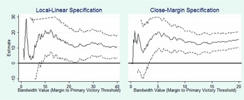
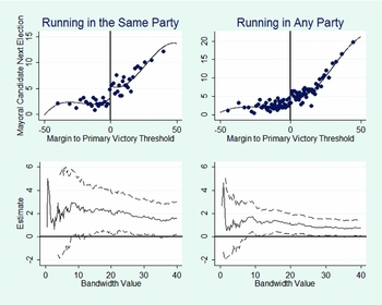
The second specification uses a narrower estimation window and a local linear-control function. This allows us to account for the relationship between the forcing variable and the outcome. In our tables, we show the results for two estimation windows: the optimal bandwidth suggested by the Imbens and Kalyanaraman (Reference Imbens and Kalyanaraman2012) test and a 10-percentage-point window around the threshold. We also graphically show the estimate for every estimation window between 0 and 40 percentage points by gradually increasing the window by 0.5-percentage-point increments and plotting each treatment effect and its 95% confidence interval.
Close Margins
The third specification uses a close margin around the threshold and excludes the control functions for the forcing variable. In tables, we show the results for a 10-percentage-point window and a 5-percentage-point window. In the Swedish case, we also plot the estimate of the treatment effect for window sizes that range between 0 and 20 percentage points.
To implement these three RDD approaches, we impose some restrictions on the sample of observations. We also show the results for estimates with and without control variables. Details about these sample restrictions and controls are explained in the context of each particular dataset.
BACKGROUND AND DATA FOR SWEDEN
Our main empirical application looks for a primary effect—as per Predictions P1–P3—in Sweden's 290 municipalities, which are political units with substantial fiscal and political power.Footnote 6 In this section, we provide background information on Sweden's municipal politics and details on our Swedish data. We pay particular attention to the system of preference voting, which was used for the first time in 1998.
Swedish municipalities are governed by a municipal council (the local parliament), which is led by the council board (the local government).Footnote 7 The chairperson of the board (the closest equivalent to a mayor) is appointed by the governing party or the largest party in the governing coalition. Specific policy areas are dealt with in subcommittees, of which the average council has seven, with chairpersons appointed by the governing majority. The board, assembly, and committee chairpersons are the most influential politicians, and the chair of the municipal council board is often the only person employed as a full-time politician.Footnote 8
On Election Day, voters are presented with ordered lists of candidates for each political party. The voters choose their preferred party ballot and also have the option to check the box next to one politician's name, which gives him or her their preference vote. Seats in the elected assembly are distributed by PR, and individual politicians are counted from the top of each party list (e.g., the top five candidates on the list each get a seat if the party wins five seats). However, if a politician amasses enough preference votes to clear the threshold,Footnote 9 he or she is guaranteed a seat. The remaining seats obtained by the party are then awarded to the politicians with the highest list ranks who do not clear the threshold.
Sweden's party system is highly stable, with seven political parties represented in nearly all municipal assemblies. Small local parties hold about 4–5% of the total council seats. The only party threshold is defined by district magnitude, which ranges from about 1.5 to 5% of the vote.
Local party organizations nominate candidates for local elections. The local party leader heads the group in formulating policy proposals and acts as its political spokesperson. It is standard procedure to place the local party leader first on the electoral ballot and appoint him or her to the top political position available to the party. The leader of the largest party in the governing majority is generally appointed chairperson of the municipal council board.
Dataset
The data for our analysis cover four waves of elections in Sweden's 290 municipalities, from 1998, when preference voting was introduced, until the 2010 election. For each election, we collected all the electoral ballots for every political party in every municipality. These ballots are registered at the Swedish Election Agency together with the personal identification code of each politician and then are stored at Statistics Sweden. With these identification codes, we can link each politician to extensive socioeconomic information from other registers. In the combined dataset, we can follow politicians over time, knowing how many preference votes they receive in each election and their rank on the electoral ballot. For the two most recent election periods, we have additional data on the political appointments held by each politician, including positions as municipal council executives, on the council board, and on committees handling specific policy areas.
Measuring Political Leadership
Our main dependent variable is a binary indicator for leadership of the municipal party at the time of the next municipal election. We define this as holding the top position on the party ballot. This top-ranked candidate is almost always awarded the top appointment in the municipal political hierarchy available to each party, which we can verify using data for appointments following the 2006 and 2010 elections. In nine cases out of ten, the chairperson of the municipal council board is the top-ranked person in the largest political party of the governing majority. In eight cases out of ten, the vice chairperson is the top-ranked person from another party, usually the largest opposition party. In seven cases out of ten, when a smaller party has a seat on the municipal council board, its top-ranked politician occupies that seat.
For a smaller sample based on the largest parties in the 2006 and 2010 elections, we also provide direct evidence of the primary effect on receiving the party's top political appointment. Specifically, we look at the appointment to municipal-council chair or to a political position with a full-time salary (which sometimes also includes the municipal council-board vice chair). These appointments are made by the local parties directly after the current election.
Measuring Politician Competence
To test prediction P2 (b), we need to measure politician competence. Our main measure is more fully explained in Besley et al. (Reference Besley, Folke, Persson and Rickne2014). It exploits data on Swedish local politicians’ labor market earnings and assumes that competence can be gauged by average income differences (over 20 years) between people with the same education, employment sector, age, and gender.Footnote 10 Besley et al. (Reference Besley, Folke, Persson and Rickne2014) show that this measure is strongly correlated with political success (measured by the probabilities of reelection and of holding positions of power, such as a council board member or committee chair). Candidates with higher competence, as we measure it, also obtain more preference votes, even when we control for list rank and other observable socioeconomic characteristics, such as education, gender, age, or being foreign born.Footnote 11 This finding indicates that voters also assess politician competence, at least partially. These correlations are verified empirically in in the Online Appendix.
Measuring Political Competition and Majority Status
To test Prediction 3, we need to measure the party's external competition and whether it is part of the municipality's political majority. Weak competition is not uncommon in Sweden, where many municipalities have been governed by the same party since 1976, the first election held after establishment of the current municipal structure. In these municipalities, preference votes might introduce an element of within-party competition even though between-party competition is nearly absent.
Because more than two parties compete in an election, it is not obvious how to measure competition. However, Swedish politics has been centered on two stable left- and right-wing blocs and has therefore been classified as a bipartisan political system (Alesina, Roubini, and Cohen Reference Alesina, Roubini and Cohen1997). The vote-share difference between these blocs is thus an appropriate measure of the main dimension of political competition (see also empirical studies, such as Svaleryd and Vlachos Reference Svaleryd and Vlachos2009). To capture the persistent component of competition, we use a three-election moving average of the (absolute) difference in bloc vote shares. A local party is defined as belonging to the majority or the opposition depending on whether the bloc it belongs to holds the political majority in the municipality.
Preference Voting Behavior
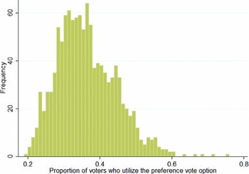
Swedish local elections have a very high turnout rate, typically 80–90%. About one-third of these voters also cast a preference vote. Surveys conducted shortly after the preference voting reform was introduced showed that voters generally understood the new system (Statens Offentliga Utredningar 1999, p. 92).Footnote 12 The most common reason for abstention, which was reported by half the respondents in various surveys, was a perceived lack of knowledge about the candidates; the second most common reason was a dislike of preference voting (Statens Offentliga Utredningar 2007, p. 68).
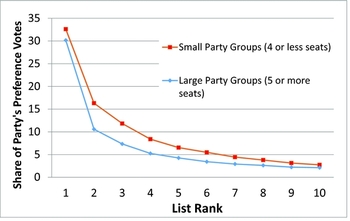
Figure 1 shows the average fraction of preference votes within party groups received by candidates on list positions 1 through 10. We divide the sample into large and small party groups, based on median representation (four representatives). On average, first-ranked candidates receive about one-third of all preference votes in small party groups and a little less in large party groups. The second-ranked candidate received less than half this number in both large and small groups. As we go down the ranks, both curves flatten out gradually. Because preference votes are concentrated on politicians at the top of the party list, most of those who pass the 5% threshold for representation for preference-vote election belong to the top group and would have been elected anyway. In fact, 19 out of 20 candidates who pass the threshold do not need their preference votes to be elected. We note that the concentration of the preference votes is consistent with strategic voting in anticipation of a downstream effect of the preference votes on leader selection—recall the short discussion in the theory section (just after Prediction P1) Footnote 13 .
Preference Votes Obtained by List Rank

We also briefly examine how preference voting differs across municipalities and election years. Figure 2 shows the municipality-election year distribution between 1998 and 2010. The four highest participation rates all come from the small northern municipality of Övertorneå. In this municipality, the Social Democrats publicly announced before the 2010 election that whoever among their top-three-ranked candidates received the most preference votes would also become the council board chair. More broadly, high-participation municipalities are all rural with below-average population. The lowest participation rate, 19%, was found in the 2006 election in Nacka, a suburban municipality just east of Stockholm. The vast majority of other low-participation municipalities are either larger cities or suburbs of Sweden's three largest cities.
Proportion of Preference Voting across Municipalities and over Time

Finally, voters for small parties on the center-right are more likely to cast a preference vote than voters for the two largest parties, the Social Democrats (on the left) and the Conservative party (on the right). Controlling for party, however, the more voters who cast a preference vote, the larger the party group in the municipal council. This correlation is interesting, because the absolute number of votes needed to clear the threshold increases with both the size of the party and the size of the municipality. Thus, the lower likelihood that their vote will be pivotal does not appear to deter voters from casting a preference vote. Further information on which kind of politicians are favored by preference voting can be found in the Online Appendix.
Estimation Sample and Control Variables
As explained in our section on statistical methodology, we define the forcing variable for our RDD analysis as, m i, p, t , the relative win (loss) margin of individual i with the highest (next-highest) preference vote over his or her closest competitor in party p in election t.
The results for the three RDD approaches described in that section are shown both with and without control variables. These variables include list rank interacted with four dummies for the party group's size in the municipal council, a dummy for being a woman, seven dummies for educational categories, a dummy for a candidate elected to parliament in t + 1, and four dummies for age categories. We also include interaction terms between a dummy for an individual being ranked at the top of the list and three dummy variables for election outcomes: (1) party p becomes part of the governing majority between t and t + 1, (2) party p is removed from the governing majority between t and t + 1, or (3) party p loses voter support between t and t + 1. If our estimates for the primary effect still hold up when these extensive controls are included, this is further evidence that our estimated relationship is causal.
Our initial sample included 6,862 election observations from competitive preference votes, where the win margin for the politician with the most preference votes is less than 50 percentage points. From this we omitted 1,266 individuals in party groups with only two elected representatives, because it is less meaningful to talk about a leadership contest in such groups. We also omitted any observation for which more than two candidates are close to the threshold of winning, because the probability of winning is less than 50% in these cases. Specifically, we excluded all observations in which the second runner-up wass within a 10-percentage-point margin from winning the most votes, which applied to 118 observations. Finally, we restricted the sample to safe seats so that we did not confound the effect of winning the most preference votes with the (potential) effect of getting elected. This was done by excluding 992 party groups where at least one of the top two preference-vote contenders was not guaranteed to be elected based on list rank (i.e., his or her list rank was lower than the number of elected candidates). Taken together, these sample restrictions left us with a final sample of 4,486 close-election observations.
RESULTS FOR SWEDEN: MAIN PREDICTION
Graphical Analysis
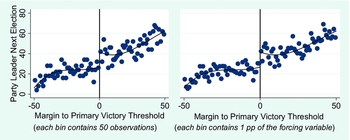
Following the “industry standard” for RDD research, we begin with a graphical analysis. Figure 3 shows binned averages of the percentage of candidates who are selected as party leaders in the next election period, Y i, p, t + 1 as a function of the win/loss margin of winning the preference vote, m i, p, t . As noted when we described the data, we set the range of m i, p, t to [–50%, 50%]. The binned averages are computed in two different ways. In the left graph, each dot corresponds to 50 observations, whereas in the right graph each corresponds to a 1-percentage-point interval for the forcing variable m i, p, t . As we cross the threshold for winning the preference vote, both graphs show a clear shift in the probability of being selected as party leader. This probability is 25 percentage points among narrow losers, but 40 percentage points among narrow winners. The primary effect thus raises the probability of becoming party leader by 15 percentage points, or by 60%, for the candidate who narrowly wins the preference vote. Thus we find strong evidence for a primary effect, as hypothesized in Prediction P1.
Graphical Analysis of the Primary Effect

Regression Analysis
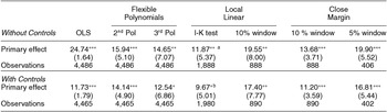
Table 1 shows regression estimates corresponding to Figure 3. For comparison, Column 1 shows the results from estimating Equation (1) using OLS. Columns 2–7 display the estimates of Equation (2),
Estimates of the Relationship between Winning the Preference-Vote Primary in Election t and Becoming Party Leader in t + 1

Notes: ***p < 0.01, **p < 0.05, *p < 0.1. Robust standard errors clustered at the party-group level are reported in parentheses. Dummy variables are scaled as 0 or 100. Control variables include three dummy variables for election outcomes: the party becomes a part of the governing majority between t and t + 1, the party is removed from the governing majority between t and t + 1, or the party loses voter support between t and t + 1. They also include the following dummy variables, included separately for the leader and the challenger: list-ranked fixed effect (for the challenger); four dummies for the size of the party group in the municipal council; a dummy for being a woman; seven dummies for educational categories; a dummy for a candidate being elected to parliament in t + 1; and four dummies for age categories, with one specifically for persons reaching retirement age before election t + 1. Bandwidth: a20.4%; b21.8%.
using the three RDD approaches outlined earlier. Columns 2–3 contain results from the control polynomial specifications, Columns 4–5 the local-linear control function specifications, and Columns 6–7 the close-margin specifications. The upper panel of the table does not include control variables, whereas the lower panel does. Each cell displays the estimated primary effect, namely β₁ in Equation (1) or (2).
The OLS results indicate that, overall, the winner of the preference vote in his or her party group is about 25 percentage points more likely to be selected as the party leader than the runner-up. However, including our extensive set of control variables cuts this estimate by more than half.
The estimates from the RDD specifications are very similar to the OLS specification with control variables, which shows that the correlation captured by the OLS estimates is indeed driven by a causal primary effect. Moreover, it suggests that the primary effect may hold external validity in the full sample of elections, including the not-so-close ones. Finally, we see that the control variables are quite efficient in capturing the selection bias in the full sample, bringing the magnitude of the OLS estimate close to that of the identified RDD estimate.
The estimates in the RDD analysis mirror the previous effect sizes observed in the graphical analysis. The two polynomial specifications in the second and third column both have large estimates of the primary effect and are statistically significant at the 1% and 5% significance levels, respectively. The I-K test in the fourth column suggests an optimal estimation window of 21 percentage points and a point estimate of 12 percentage points, which is also statistically significant at the 5%level. The local-linear specification with the 10% estimation window in the fifth column gives a larger point estimate, which reflects fitting the control function to observations closer to the threshold. The close-margin specifications in the sixth and seventh column have a similar pattern, with a larger point estimate for the narrower estimation window, and both estimates significantly different from zero at the 1% level.
When we include the large set of controls in the lower panel of the table, the estimates of the primary effect barely change for our RDD approaches, unlike the naive OLS estimates. For the specifications that use a wide estimation window, we also see a reduction in the standard errors. The estimates’ robustness to a large set of variables strongly related to a candidate's share of preference votes, as well as his or her selection as local party leader, strongly supports the claim that our RDD estimates of the primary effect are indeed causal.
Figure 4 shows estimates for the local-linear and close-margin specifications over numerous sizes of the estimation window. The solid line is the estimated treatment effect that corresponds to each window size, and the dotted lines represent the 95% confidence interval. The confidence intervals are censored and only shown in the interval [-10, 30]. It is hard to obtain precise estimates for very narrow windows around the threshold and thus for very small estimation samples. However, at reasonable sample sizes, the estimates are remarkably stable and significant at the 95% level for all bandwidths. The results clearly show that there is a substantial primary effect.
Estimates of the Primary Effect by Estimation Bandwidth

Robustness Checks
To validate our identifying assumption that preference-vote winning is as good as random around the threshold, we conduct a large set of robustness checks. We summarize these tests here; a more detailed explanation with tables and figures is available in the Online Appendix. Our first check is the McCrary test (McCrary Reference McCrary2008) for balance in the density of observations around the threshold, which we use to verify that the first-ranked candidate on the list is not more likely to become the preference-vote winner close to the threshold. Restricting the sample to only candidates who are the party leaders in period t, the McCrary test shows no difference in the number of times that these current leaders win or lose close contests.
Second, we check that variables that should not be systematically affected by the treatment are indeed balanced on the two sides of the threshold. To do that, we perform graphical analyses as well as placebo regressions on four relevant predetermined covariates: being the current leader, the individual's current list rank, the politician's sex, and his or her years of education. This analysis strongly suggests that covariates are balanced around the threshold. There is no significant difference in the chosen characteristics for individuals who narrowly win or lose close contests.
In a third check, we create so-called placebo thresholds at false values of the forcing variable. In this analysis, we only find a significant treatment effect at the true threshold. Taken together, all the robustness checks provide very strong support for our identifying assumption.
Validation of the Party Leader Measure
To verify that preference voting causes a reallocation of political power rather than a mere reshuffling of candidates on the list, we use data on specific political appointments. For the largest party of the political majority in each municipal assembly, we have information on exactly which politician was appointed chair of the municipal council board, an appointment that is made immediately after the general election. We also use data that indicates exactly which politician holds a full-time political employment, which is a strong indicator of influence. We include parties that have appointed a single full-time politician. This can be either the mayor (for the largest majority party) or the vice mayor (for the largest opposition party). The vice mayor is a full-time politician in about 40% of the municipalities in our sample, and the mayor is nearly always full-time.
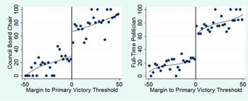
For this estimation, we only have data for two waves of elections. This, plus the restriction to parties that get to nominate the council-board chair or one full-time politician, limits the sample to 496, or 640, observations.Footnote 14 This makes our estimates of the primary effect less precise and more sensitive to the precise specification. Due to the smaller sample size, we increase the bin size to 2 percentage points of the forcing variable in the graphical analysis shown in Figure 5.
Graphical Analysis of the Primary Effect on Municipal Council Board Chairpersonships and Full-Time Politicians

The figure shows a striking shift in the probability of becoming the chair of the council board, as well as becoming a full-time politician, as we cross the threshold for winning the preference-vote primary.
Around 30% of the close losers are appointed chairperson after the election, compared to around 70% of the close winners. Around 30% of the close losers become full-time politicians versus 60% of the close winners. Thus, preference-vote winning more than doubles the probability of obtaining a position of undisputed political power.
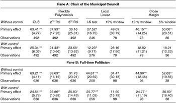
The regression analysis in Table 2 corroborates the graphical evidence by showing significant primary effects in most RDD specifications for both outcome variables. Because of the small sample sizes, we cannot include the full set of controls; therefore we use a single dummy variable for the current list leader (the strongest predictor of becoming the council chair) and for the preference votes received by a candidate. Still, the estimates should be interpreted with caution, because they are sensitive to both the specification and the control for being the current leader. Despite this uncertainty in the magnitude of the primary effect, the results validate our main finding: Political parties use the distribution of preference votes to decide which politicians to promote.
Estimates of the Relationship between Winning the Preference-Vote Primary in Time t and Being Appointed Chair of the Municipal Council (or a Full-Time Politician) at t + 1

Notes: ***p < 0.01, **p < 0.05, *p < 0.1. Robust standard errors clustered at the party-group level are reported in parentheses. Dummy variables are scaled as 0 or 100. The control variable is a dummy for being the party leader (i.e., top ranked on the party list) in the current election. Bandwidth: a27.5%; b30.4%. c17.4%; d20.6%.
List Rank rather than Top Rank as the Outcome
As a final piece of evidence, we can also use list rank (as opposed to top rank) in election t + 1 as our outcome variable to further show that preference votes are used to determine political promotion. The analysis, which appears in the Online Appendix, shows that winning the most preference votes results in a lower list rank (i.e., a safer seat) in the next election. The results in this section strongly support the presence of a primary effect, as hypothesized in Prediction P1.
RESULTS FOR SWEDEN – ADDITIONAL PREDICTIONS
In this section, we look for support for the auxiliary Predictions P2 and P3 about how the primary effect hinges on individual candidate features and political contexts.
Prediction P2 (a) – The Primary Effect Conditional on Party Support
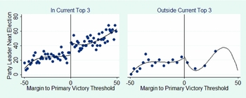
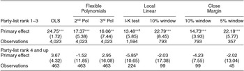
To shed light on Prediction P2, we differentiate our estimates of the primary effect to check for limitations in voter influence. We first check whether this effect is smaller for candidates with lower list ranks, for the reasons discussed in the theory section. Figure 6 shows the graphical results of our RDD in these two samples. The baseline finding in Figure 3 is replicated in the left graph, based on the sample of candidates ranked in the top three. Among these three politicians, winning the most preference votes dramatically raises the likelihood of becoming party leader. The right graph shows that candidates below the top three do not experience the same career boost. Although the sample is smaller, there is no indication that close winners have a larger average likelihood of becoming party leader than close losers.
Graphical Analysis of the Primary Effect on Party Leadership in the Next Election

Table 3 contains the results from applying the RDD to the subsamples based on list rank. The regressions tell a clear story and validate the inference from the graphs. The primary effect exists only for politicians who are already part of the party elite. In the Online Appendix, we analyze still smaller samples defined by individual list rank. This analysis shows that the primary effect is of a similar size and is positive for candidates ranked first, second, and third, but not for lower ranks. Thus our baseline result does not stem from voters simply supporting the party's top candidate. Instead, parties reallocate the top post to second- and third-ranked candidates when they win the most preference votes.
Estimates of the Relationship between Winning the Preference-Vote Primary in Election t and Becoming Party Leader in t + 1, by Party-List Rank

Notes: *** p < 0.01, ** p < 0.05, * p < 0.1. Robust standard errors clustered at the party-group level are reported in parentheses. The table shows estimates of the primary effect, by list placement at time t. Bandwidth: a19.1%; b24.3%.
Therefore, the analysis strongly suggests that a candidate must reach a high enough position in the party hierarchy to benefit from winning the most preference votes. Thus voters do have influence over party leadership, but only within a predetermined pool of candidates. It is as if candidates first have to pass a vetting process before they are eligible to participate in the primary. In this sense, voter support is a complement to, rather than a substitute for, party support.
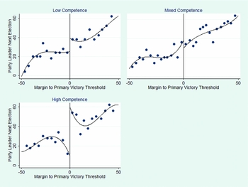
Prediction P2 (b) – The Primary Effect Conditional on Individual Competence
To test the prediction that parties are more responsive to preference-vote winning when candidates are similar, we turn to an analysis of the primary effect by competence. Here, we split the baseline sample into three groups. Using the median of our competence measure based on income residuals, we separately examine races in which the winner and runner-up are (1) both competent, (2) both mediocre, or (3) one is competent and the other mediocre. As previously, we start with a graphical analysis, as shown in Figure 7. When comparing the graphs for the three subsamples, we see a clear indication of a primary effect only when the two candidates have the same competence level. The primary effect seems to be particularly large when both contenders have high competence.
Graphical Analysis of Heterogeneous Primary Effects by Candidate Competence

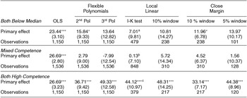
The regression analysis in Table 4 sheds more light on how the treatment effects differ across the three samples. When both candidates are competent, the estimated primary effect is always significantly different from zero. When one candidate is competent and the other mediocre, the point estimates are close to zero and never significant. When both candidates are mediocre, the point estimates are consistently positive, but are only statistically significant in two specifications.
Estimates of Heterogeneous Primary Effects Competence

Notes: ***p <0.01, **p <0.05, *p <0.1. Robust standard errors clustered at the party-group level are reported in parentheses. The table shows the estimated primary effect, by individual competence measures being above and below median competence as measured by average income residuals. Bandwidth: a21.13%; b26.8%; c21.8%.
Together, these results support Prediction P2 (b) that the primary effect is stronger for candidates with similar individual characteristics. As discussed in the theory section, this is consistent with a learning model in which parties respond in larger measure when they learn about the relative voter popularity of two candidates of similar competence. However, no such response is present when the information concerns candidates of dissimilar competence.
Prediction P3: The Primary Effect Conditional on Political Context
Which party groups drive our finding that parties, on average, respond strongly to preference votes when distributing power? It is particularly important to check how party response relates to political competition. As noted by Hirano and Snyder (Reference Hirano and Snyder2013), in the U.S. context primary elections are mostly needed when competition between political parties is poor.
As explained in our theory section, we do not want to take a strong stand on the effect of internal and external party competition so we divide the party groups into four different subsamples. We base these on the measures of majority status (majority or opposition) and external political competition (above or below the median), as defined in the institutional background. The RDD analysis of preference votes and party leadership again starts with graphs.
Figure 8 clearly shows that the primary effect is the largest in governing parties of low-competition municipalities. In this subsample, we see a large shift in the probability of becoming the local party leader as the winning threshold is crossed. In municipalities with high competition, an effect—although a weaker one—appears to be present in both majority and opposition parties. Finally, opposition parties in low-competition municipalities show no sign of a primary effect. These parties have a low probability of exerting political influence and few important positions to distribute, so we would expect there to be little internal competition for top positions.
Graphical Analysis of Heterogeneous Primary Effects by Political Context

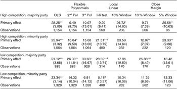
The regression results, presented in Table 5, reinforce the visual impression of the graphical analysis. We see a large primary effect in majority parties in low-competition municipalities. The estimated primary effect (the increase in the probability of becoming party leader from achieving victory in the preference vote) varies between 20 and 30 percentage points across specifications. These estimates are also significant at the 10% level in half of the regression specifications. In the high-competition subsamples for majority and minority parties, the estimated primary effect is not as consistent, but always has a positive sign. Opposition parties in low-competition municipalities show no sign of a primary effect.
Estimates of Heterogeneous Primary Effects by Political Context

Notes: *** p < 0.01, ** p < 0.05, * p < 0.1. Robust standard errors clustered at the party-group level are reported in parentheses. The table shows estimates of the primary effect by majority status of the party and political competition. Dummy variables are scaled as 0 or 100 to give results in percentage terms. Bandwidth: a24.5%; b17.5%, c16.8%; d16.4%.
These results mostly support Prediction P3. The clearest empirical regularity shows that preference voting can serve a similar role as the introduction of primary elections in the United States: to introduce individual electoral accountability within dominant parties in localities where political competition is weak.
BACKGROUND, DATA, AND RESULTS FOR BRAZIL
Brazil has approximately 5,500 municipalities. According to federal law, all municipalities hold elections on the same day and every fourth year for municipal councils and mayors, Municipal councils have between 9 and 55 members, and the council members are elected by proportional representation of parties and/or electoral coalitions. The mayor (perfeito) is the dominant figure in municipal politics and is directly elected by plurality rule in an at-large election.
Political parties are responsible for nominating council and mayoral candidates. People are eligible for nomination if they have lived in the municipality and been a member of the party for at least one year. Importantly for our study, political parties select a single nominee for the mayoral election, a rule that that has produced “bitter battles” within parties (Hunter Reference Hunter2010). Candidates on the open list in the council election are not ranked by the party, and the elections are centered more on individual candidates than on political parties. In both elections, candidates are given a unique electoral ID code, and preference votes are cast by punching this code into an electronic voting machine.
Political parties can run independently or form an electoral coalition with other parties. In the latter case, seats are allocated to the coalition as a whole rather than the party. For both parties and coalitions, politicians are given seats based on a ranking determined by their number of preference votes. Participation in a coalition increases the probability of obtaining seats, because seats are distributed to the entire coalition and Brazil's seat allocation formula (D'Hondt) gives an advantage to large parties and/or coalitions, in particular when the council is small. Coalitions only pool the votes of the parties, but are not a means of joint candidate nominations.
The dependent variable in our analysis of Brazil is whether a candidate becomes a candidate for mayor in the next election.Footnote 15 We define this outcome in two ways. The first is a binary indicator for the council member becoming a mayoral candidate for the party that he or she represents in the council. In this estimation we restrict the sample to parties that actually fielded a mayoral candidate in the next election. The second specification of the outcome is an indicator for becoming a mayoral candidate for any political party. In Brazil, politicians frequently change political parties. Thus, we want to examine if our result holds up when we allow for such changes. If they do, this suggests that preference-vote losers do not shift parties to become mayoral candidates in other parties, so that both winners and losers have an equally large probability to become mayoral candidates, albeit in different organizations.
Our data come from the 2000, 2004, 2008, and 2012 elections.Footnote 16 Sample restrictions mirror those in the analysis of Sweden. We thus only include party groups with at least three elected representatives and exclude all party councils where the preference-vote share of the second runner-up is within 10 percentage points of the top two preference-vote shares. Figure A8 in the Online Appendix shows the distribution of preference votes in this sample of local parties. Because list ranks do not exist, we plot the proportion of preference votes against preference-vote rank. As in Sweden, preference votes are concentrated on a few politicians, especially in small party groups.
Figure 9 shows the primary effect on becoming a mayoral candidate. The upper part shows the RDD graphs for each specification of the outcome variable. Because the sample size is much larger than in the Swedish case, we use 250 observations in each bin of the graph. We see clear evidence of a primary effect; that is, the probability of becoming a mayoral candidate increases as we move horizontally in the figure and cross the threshold where a politician wins more preference votes than his or her main competitor (a positive “margin to primary victory threshold”). Although the overall probability that a council member becomes a candidate for mayor is quite low, as indicated by the low values on the y-axis, the probability clearly increases as we cross the threshold. The top left graph plots the probability of becoming a mayoral candidate of the politician's own party in period t + 1, conditional on that party fielding such a candidate. A close winner (a candidate immediately to the right of the vertical line) has a probability of becoming a mayoral candidate that is about two percentage points higher than the probability of a close loser (immediately to the left of the vertical line). The top right graph plots the probability of becoming a mayoral candidate for any party in period t + 1. Here, too, we see a jump, albeit smaller, as we cross the threshold for winning the preference vote.
Graphical Analysis of the Primary Effect in Brazil

The lower part of the figure shows the estimated treatment effect for varying sizes of the estimation window, ranging from 0–40 on the forcing variable. These estimates come from the local-linear specification. The left plot shows that the probability of becoming a mayoral candidate in the politician's own party in period t + 1, conditional on that party fielding such a candidate, increases about two percentage point for a politician who wins the most preference votes. When other parties are included, the probability increases by just over one percentage point. These estimates are stable and statistically significant across reasonable estimation windows. In the Online Appendix (Table A4) we also show the corresponding regressions. These are organized the same way as in the Swedish case and corroborate the results displayed in the upper part of the figure.
How do we interpret the fact that the primary effect is larger for the politician's own party? A simple interpretation is that winning the preference vote creates an advantage in the party for which the preference votes were originally cast, but not in any other party. Interestingly, this accords well with our reasoning that the key mechanism generating the primary effect is found at the party level (in promotion decisions) rather than at the candidate level (for example, via higher career ambitions and efforts). Furthermore, it testifies to the fact that party allegiances are quite weak in the Brazilian municipalities, where party switching is commonplace (Anagol and Fujiwara Reference Anagol and Fujiwara2014). For example, a candidate who fails to gain the nomination in his or her own party can simply switch to another party. This dampens the estimated primary effect when running in any party is used as the outcome.
DISCUSSION AND CONCLUSIONS
We show how political parties use the distribution of preference votes across candidates on the electoral ballot in making subsequent decisions on career advancement. Semi-open or open lists allow voters to signal candidate popularity to parties, which internalize these signals in their nomination procedures. We document such a primary effect both in Sweden's system with semi-open lists and in Brazil's open-list system.
Our results offer additional insights into the impacts of preference voting. First, they suggest that preference voting can at least partly overcome the problem of poor popular accountability of the indirect leader selections in PR systems. Even if preference votes are strongly skewed toward high-ranked politicians (who are ensured a legislative seat without them), preference votes can still make or break politicians’ careers within the elected body. This observation is important against the backdrop of recent work, which argues that political power in many PR systems is increasingly moving into the party executive (Poguntke and Webb Reference Poguntke and Paul2005). Indeed, our empirical results show that the distribution of preference votes helps shape the allocation of executive positions.
Second, the results fly in the face of the idea of “wasted” preference votes. In the conventional view, voters are wasting their preference votes on high-ranked politicians in semi-open list systems, because these politicians are already ensured a safe seat. Similarly, votes for candidates who win their seats with a large margin in open-list systems are also seen as largely wasted. We show that these supposedly wasted votes appear to have considerable downstream effects on appointments to leading party positions. At a general level, this finding is reminiscent of a recent branch of voting theory, in which votes can have a downstream signaling effect on policy (Meirowitz and Shotts Reference Meirowitz and Shotts2009; Piketty Reference Piketty2000; Razin Reference Razin2003). It is also in line with the empirical findings of Anagol and Fujiwara (Reference Anagol and Fujiwara2014) that finishing second instead of third in plurality elections affects a candidate's future political success.
Third, our results are particularly important in helping us understand semi-open list systems. Previous research has concluded that these systems have been evaluated as little more than “closed lists in disguise” (Andeweg Reference Andeweg, Gallagher and Mitchell2005; De Winter Reference De Winter, Gallagher and Mitchell2005; Farrell Reference Farrell2001; Mueller Reference Mueller, Gallagher and Mitchell2005). However, our results show that the allocation of preference votes can lead to widely different promotion patterns in semi-open-list systems compared to closed-list systems.
The interplay between voters and parties in the context of preference voting is an exciting topic for future theoretical and empirical research. Previous work on personal vote-seeking incentives could be expanded to consider the link between parties’ exploitation of preference-vote outcomes and the efforts of political candidates and leaders to pursue these votes. If parties use preference votes to guide top appointments, this will likely increase candidate vote-seeking behavior, such as deviations from the party line or bill initiation (see Bräuninger, Brunner, and Däubler Reference Bräuninger, Brunner and Däubler2012, and Crisp et al. Reference Crisp, Olivella, Malecki and Sher2013). This insight might redirect our attention from reelection incentives to appointment incentives, which in turn should change the focus from the party's marginal candidates to its elite representatives. Individual vote-seeking behavior can sometimes be detrimental to the democratic system, as stressed by Chang and Golden (Reference Chang and Golden2007) in the Italian case. However, our results for Sweden suggest that preference voting has given voters more influence while letting parties remain the ultimate gatekeepers of final ballot nominations, a seemingly fortunate mix of voter and party control. A comparative perspective will therefore be important in future research.
It is also possible that primary effects could directly affect political behavior, beyond the indirect effect via higher vote-seeking incentives. If top appointments are based on preference votes, top politicians might view themselves as more personal than party representatives (Davidsson Reference Davidsson2006). This begs the question of whether party leaders appointed via preference votes behave differently in office. Do they, for example, shift the policy focus from the party line to their own preferences, or do they communicate differently with voters? Such consequences should also be considered in normative judgments of preference-voting reforms. These are important topics for further research.
Let us finally consider some points that emanate from our auxiliary Predictions P2–P3. In the Swedish case, our empirical results show that the primary effect is only present when the candidates have similar levels of competence, and it is particularly strong when both are highly competent. This suggests that preference votes are a complement to (rather than a substitute for) other selection criteria.
We also find support for our prediction that the primary effect should increase with both external political competition and internal party competition. The first finding is consistent with the idea that office-maximizing parties can use preference votes in their selection process to improve their electoral prospects. The second finding mimics research results on the voluntary adoption of primaries in U.S. states and in Latin America by local political party organizations, where strong parties adopted primaries to avoid intraparty conflict. That we observe a similar dynamic after the introduction of preference voting implies that such reform may boost leadership accountability as voters get an opportunity to “throw the rascals out” within the dominant party.
SUPPLEMENTARY MATERIALS
To view supplementary material for this article, please visit http://dx.doi.org/10.1017/S0003055416000241





Comments
No Comments have been published for this article.