1. Introduction

The notion of “path dependence” is becoming increasingly popular among scientists in order to explain and emphasize historicity, that is, the idea that history matters in various processes. Most at home in cases involving the lock-in of technologies (the QWERTY keyboard being perhaps one of the most discussed examples), path dependence lies at the basis of several historical turns in social sciences and has recently made its way into the field of biology.Footnote ¹ But we are far from a well-developed theory of the phenomenon of path dependency, and some conceptual tensions have yet to be addressed. The following two propositions (often) constitute the essence of path dependence:

Proposition A is true, but I will show that it needs to be further specified in order to capture the heart of path dependence. Proposition B, on the other hand, is more problematic. The notion of “irreversibility” possesses many faces (Gould Reference Gould1970; Macbeth Reference Macbeth1980; Bull and Charnov Reference Bull and Charnov1985; Denbigh Reference Denbigh1989), and some of them clearly conflict with path dependence. Section 2 will show why an unspecified interpretation of proposition B can be problematic. Section 3 will offer a fuller definition of path dependence, and section 4 will look at alternative interpretations of proposition B based on evolutionary biology.

2. Entropic(-like) Irreversibility

Proposition B cannot be interpreted, for instance, in the context of the second law of thermodynamics (SLT), an archetypical example of irreversibility in natural sciences. The SLT entails the existence of a function, entropy, which increases monotonically until it reaches its maximum value at the state of thermodynamic equilibrium (Sklar Reference Sklar1995). This law entails irreversibility because the entropy of an isolated system can increase (if in a nonequilibrium state) or remain constant (at entropic equilibrium), but it can never decrease. The result is an asymmetrical dynamic, a fundamental difference between past, present, and future. Interpreting proposition B in terms of entropic irreversibility would raise two important problems. First, the SLT applies only to isolated systems. This essential criterion does not apply to socioeconomical and biological contexts in which path dependence appears. Second, the entropic equilibrium state toward which isolated physical systems evolve is unique. This constitutes a violation of proposition A.

A more promising avenue consists of interpreting proposition B in terms of evolutionary irreversibility, which does not apply to isolated systems. David (Reference David, Garouste and Ioannides2001, 2), for example, describes path dependence as a property of contingent, nonreversible dynamic processes, including a wide array of processes that can properly be described as evolutionary. Unfortunately, David offers very little information as to how to interpret irreversibility in this evolutionary context. But, more important, not any interpretation of evolutionary irreversibility will do.

The theory of evolution by natural selection entails an entropic-like irreversibility that follows from Fisher's fundamental theorem of natural selection (FTNS), which says that the rate of increase in fitness of any organism (i.e., average fitness of population) at any time is equal to its genetic variance in fitness at that time (Fisher Reference Fisher1956, 37). This theorem is still the object of vivid debates (that I cannot summarize here; see Edwards Reference Edwards1994 and Okasha Reference Okasha2008), but if it were true, it would entail irreversibility. Variance in a population can be positive when a population is not homogenous or null for homogenous populations, but it cannot be negative. Therefore, average fitness can only increase (for nonhomogenous populations) or remain constant (for homogeneous populations), but it cannot decrease. This incited Fisher to draw an analogy with the SLT. Many, Fisher included, have questioned the strength of this analogy (Barrett and Sober Reference Barrett, Sober and Savitt1995; Gould Reference Gould2002; Okasha Reference Okasha2008), and it has been suggested that it may simply be untenable. After several years of debate about the exact meaning of the FTNS, biologists seem to agree that we should interpret the theorem as establishing a partial relationship between the genetic variance and the average fitness of populations. In fact, the modern interpretation of the FTNS reads “the rate of change at any time in average fitness of a population undergoing natural selection is equal to the additive genetic variance at that time” (Edwards Reference Edwards1994, 20).

This excludes changes in average fitness due to environmental fluctuations, which can reduce the average fitness. A given set of genes generally takes different fitness values in different environments. Thus, changing the environment would typically cause the average fitness of a so-far-well-adapted population to diminish. Moreover, even if we were to assume stability of the external environment, we would still have to deal with the fact that natural selection, by affecting gene frequency, can also cause the average effects of genes on the population fitness to decrease (epistasis; Ewens Reference Ewens1989). So, in addition to a constant external environment, the FTNS also needs a frequency-independent fitness contribution of genes in order to be verified.

The latter conditions have at least two important implications. First, they impose a very strict reading of the FTNS and reduce significantly its applicability. It follows from the modern interpretation that irreversibility may not actually be realized in many systems. Okasha, for instance, suggested, “Evolution by natural selection does not actually have an arrow of time; from a sequence of successive state descriptions of an evolving population one could not deduce the direction of time, as one could from a sequence of state descriptions of a closed thermodynamical system” (Reference Okasha2008, 346).

One could reply, however, that the second law, too, is an idealization requiring strict conditions. As mentioned above, the SLT concerns only isolated systems. So we would observe an increase in average fitness with time if we were able to produce the right kind of circumstances.

Second, the evolutionary dynamics of a population in the conditions entertained by Fisher will typically describe converging trajectories toward a global equilibrium (Gavrilets Reference Gavrilets2004). This form of evolutionary irreversibility is literally opposed to path dependence because it, too, violates proposition A. So, at face value, interpreting proposition B in terms of the evolutionary irreversibility entailed by the FTNS will not work. These examples show that our understanding of path-dependent phenomena would benefit from a more careful analysis of irreversibility and a clarification of exactly how it relates (or not) to path dependence. I will explore two ways in which proposition B can be successfully interpreted, both entailing a surprising conclusion. But we first need to take a closer look at path dependence.

3. Path Dependence

I conceive of “path dependence” as the form of historicity happening in stochastic information-preserving processes.Footnote ² Let me clarify this latter notion by way of example. The marble released from anywhere inside the edge of a hemispherical bowl will eventually immobilize at the bottom of it. The outcome of this process is independent of the marble's initial position. If someone were to find the marble at the bottom of the bowl, there would be no way to know anything about the initial position of the marble. Information about the initial position is erased at equilibrium. Things would be different if the bowl had two deep wells. Finding the marble at the bottom of one of the wells tells something about the past. The observer can broadly infer the initial position of the marble on the rim based on what well she finds the marble in. So (some) information about the past is preserved in this case.

The bowl with one well exemplifies an information-destroying process because of the existence of a unique, global equilibrium. The bowl with two wells represents an information-preserving process because of the existence of multiple equilibria and a relation of causal dependence between past and present states. Spelled out more generally, an information-preserving process possesses three essential qualities:

1. 1. Multiple possible pasts: alternative initial conditions or trajectories from a given starting point;

2. 2. Multiple possible outcomes at a given instant;

3. 3. Causal dependence: the probability of outcomes must change as a function of the initial condition or path realized at a particular occasion.

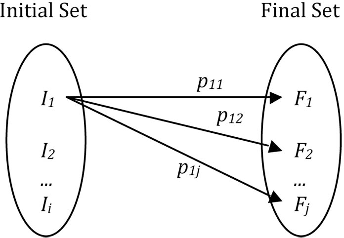
Two forms of historicity can be represented with conditions 1–3: “dependence on initial conditions” and “path dependence.” I will begin with the former. Imagine a system admitting of a set of possible initial states and another set of possible final states (fig. 1). Each element of the initial set maps into the different elements of the final set with various transition probabilities p _ij ranging from zero to one. These transition probabilities can also be conceived of as conditional probabilities, , defining the probability of outcome j given initial state i. Applying our definition to this setting, we would say that a process is information preserving if the probability of an outcome j given initial condition i is different from the probability of that same outcome j given another initial condition, ; that is, . Conversely, a process would be information destroying if the probability of a given outcome remains independent, regardless of what past conditions is realized; that is, (where is any initial state different than i).

Figure 1

Elements of an initial set mapping into elements of a final set with different probabilities p _ij. For the sake of clarity, the probabilities of only one element of the initial set are represented here.

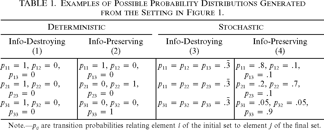
Table 1 provides examples of probability distributions corresponding to situations where information from the past is either preserved or destroyed. Although expressed in probabilistic terms, the conditions of information-preserving processes can explain how information is preserved or lost in deterministic settings. In the latter cases, only one arrow will have probability = 1; that is, only one possible outcome per initial state would be possible (as in table 1, cols. 1 and 2). Column 1 corresponds to an information-destroying process because only one outcome (F ₁) obtains, regardless of which initial state happens to be realized. Column 2, on the other hand, gives an example of an information-preserving process because different initial states consistently yield different outcomes. Note that the only way in which a deterministic process can yield multiple outcomes is by wiggling the initial conditions. This means that historicity in deterministic processes reduces to the principle of dependence on initial conditions.

Table 1Examples of Possible Probability Distributions Generated from the Setting in Figure 1.

Deterministic		Stochastic
Info-Destroying (1)	Info-Preserving (2)	Info-Destroying (3)	Info-Preserving (4)

Note p _ij are transition probabilities relating element i of the initial set to element j of the final set.

Things are different for stochastic processes. We can still obtain independence on initial conditions (col. 3) or dependence on initial conditions (col. 4), but divergent outcomes can also result from wiggling the entire series of events connecting a starting and an end point. This allows for a different form of historicity: path dependence.

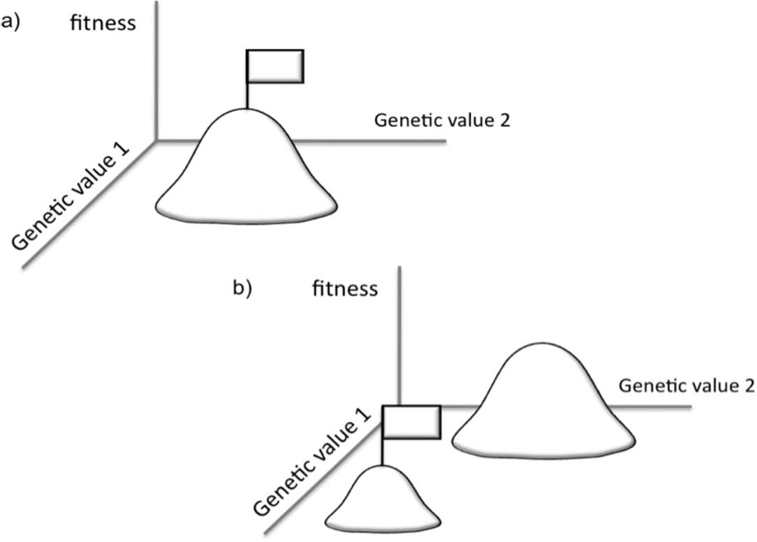
To make the distinction between path dependence and dependence on initial conditions more obvious, let us consider the example of two initially identical populations evolving in the same environment. Imagine a situation where there exists but one optimal solution to an evolutionary problem. This can be represented with a Fujiyama-like adaptive landscape (fig. 2a). The x- and z-axes represent the range of genotypes under investigation, and the y-axis represents the adaptive values (fitnesses) of the various genotypes. Given sufficient time, a population described by these genotypic variables and adaptive values would ascend by natural selection to the unique peak of the landscape, where it would then rest, regardless of which trajectory the population has taken. If we had no record of the process, then we would have no idea what route it took to that outcome. This type of process is therefore information destroying (and path independent).

Figure 2

Examples of adaptive landscapes with one (a) or two (b) peaks. The flags represent realized outcomes. See the text for explanation.

The latter conclusion holds only for the equilibrium state. In fact, history will (possibly) matter along the way, too. Suppose that initially identical populations can have transient divergent mutational histories; that is, the order and timing of mutations change from one population to another but converge at the end. Information from the past can be retained before a population reaches equilibrium, and the process would be transiently path dependent. Thus, including transient path dependence in the realm of historicity is possible if we add, as I have done in condition 2, a temporal component in the definition, saying that there must exist multiple possible outcomes at a given instant. A definition focusing only on the long-term (final) outcome will not be able to conclude that path dependence applies here.

We can contrast this with long-term (by opposition to transient), path-dependent evolutionary processes. Wright's typical vision of a fitness landscape offers such a case. For a particular population in a particular environment, there might be more than one solution, that is, alternative evolutionary stable strategies. In the context of fitness landscapes, we can compare these stable strategies to separate equilibrium states (two genetic combinations of relatively high adaptive value, separated in genotypic space by forms of lower value and not traversable by mere natural selection; fig. 2b). In this case, the evolutionary outcome will depend on the stochastic variations in the genotype frequencies (drift) and history. The latter becomes important because the genotypic starting point together with the mutational history can make a difference to which peak a population will climb. A population might come to rest on one rather than the other peak for the simple reason that mutational changes in that direction happened to arise and were selected, whereas mutational changes in the direction of the other peaks did not occur and could not be selectively accumulated.

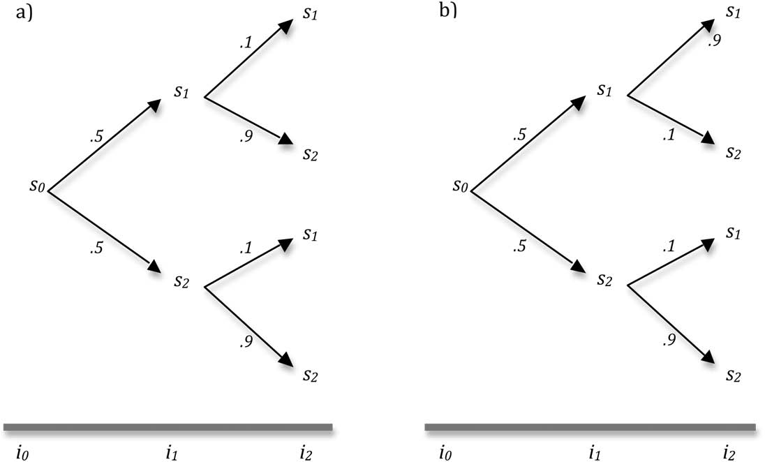
Note, however, that the possibility of having multiple outcomes is insufficient for history to matter because the probability of reaching one or another outcome could be independent of changes in past conditions. In other words, condition 2 could be met without condition 3. For instance, if we could create an experiment in which the same population is repeatedly placed in the same environmental conditions, and there existed different ways to become adapted to this environment (i.e., multiple peaks), then a different outcome would possibly obtain for each run.Footnote ³ Suppose the simple situation where the population starts in state s ₀ and can possibly evolve toward states s ₁ or s ₂ (consider fig. 3). One can think of these states as alternative peaks in a fitness landscape. If we discover that the probability of reaching one peak or another is always the same, regardless of the mutational trajectory taken by the population, then history would not matter (as in fig. 3a). Figure 3b, on the other hand, represents a path-dependent evolutionary process. If going from one peak to another implies that the population has to go through a series of less fit genotypes, then natural selection will most likely preclude jumping from one state to another. Populations will thus get locked into certain states depending on the mutational history they took.

Figure 3

Branching tree diagram representing possible paths for a population starting at initial state s ₀. a, Path independence follows from this graph because of the independent probability of outcomes s _i at instant i ₂. b, Path dependence follows from this tree because the probability of outcomes changes with the path taken by the process.

The important lesson from this simple example is that saying that history matters means more than things could have been otherwise, because we could be in a situation where the probability distribution of outcome is independent of past states. This is why proposition A insufficiently characterizes path dependence and why condition 3 is essential to any form of historicity.

History can also matter to different degrees under this account, depending on the difference in the conditional probabilities of a certain outcome given different paths.Footnote ⁴ Referring to figure 2b, we could say that history matters a lot when the probability that a population climbs the lower peak, given evolutionary path p, is much higher than the probability that it reaches the same (lower) peak, given evolutionary path (where p corresponds to early mutations in direction of the lower peak, and corresponds to early mutations in the direction of the higher peak). Figure 3b could represent this type of scenario. To the contrary, we would say that history does not matter as much if the probability of reaching a particular peak given p was not much different from the probability of reaching the same peak given . More generally, if, at a particular instant, the probability of reaching a particular outcome given one path is very different from the probability of reaching the same outcome given a different path, then we have a high degree of path dependence. On the other hand, we have a lesser degree of path dependence if the difference in the conditional probabilities of a given outcome is small. At the end of the continuum we obtain complete path independence (as in fig. 3a and col. 3 in table 1), where changing the past makes no difference to the conditional probability of a given outcome.

4. Irreversibility

We saw in section 2 how a conflict arises when we try to interpret proposition B in terms of entropic(-like) irreversibility. The latter applies to processes with a unique equilibrium, and thus violates proposition A. But this follows only if we do not have an instant-relative conception of path dependence. The account offered above supplies a solution to this problem. By treating path dependence as an instant-relative property (condition 2), we allow for transient path dependence, which is compatible with entropic-like irreversibility. In other words, proposition B is false if we focus only on the long-term outcome, but it may be true if we consider the property of transient path dependence. Note, however, that this conclusion holds only as long as conditions 1 and 3 are also met.

In a discussion of the path-dependent nature of evolution, the biologist Eörs Szathmáry suggests that “at the population level path dependence entails that the probability of going back to some previous state decreases with time, or that switching to a state that could have easily been reached, had the population taken a different turn previously, is becoming increasingly improbable as time goes on” (Reference Eörs, Wimmer and Kössler2006, 141). In other words, path dependence entails contingent irreversibility” (Maynard-Smith and Szathmáry Reference Maynard-Smith and Szathmáry1995). Returning to a previously visited state becomes increasingly improbable with time because of the influence of conditions and preconditions that are individually or jointly improbable.Footnote ⁵ Unlike entropic irreversibility, Szathmáry's description assumes a branching process. The probability of a past state diminishes as a function of the time spent on a certain path, but it could have been more likely to occur had the population taken a different path (or turn).

Contingent irreversibility is perhaps the most common notion of irreversibility in the biological literature. It goes back at least to Louis Dollo, who during the late nineteenth and early twentieth centuries provided theoretical grounds and empirical evidence of the irreversibility of macroevolutionary changes. Typically, Dollo would emphasize irreversibility by arguing that species that have to adapt more than once to similar environmental conditions never totally re-evolve their ancestral traits. Suppose that a lineage existing in environment E evolves adaptation A. Then, the environment changes to and, after a certain time, the lineage evolves a different trait, . 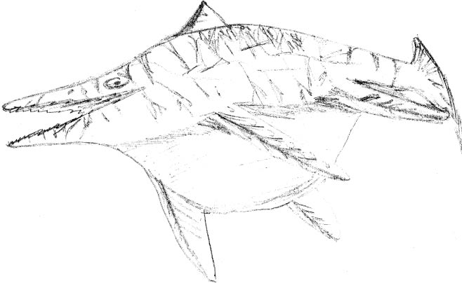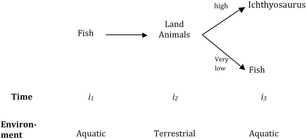What would happen if the environment were to return to state E? According to Dollo “[a species] never returns exactly to a former state, even if it finds itself placed in conditions of existence identical to those in which it previously lived. But by virtue of the indestructibility of the past it always keeps some trace of the intermediate stages through which it has passed” (Gould Reference Gould1970, 196). So, for Dollo, the irreversible nature of the evolution of organisms is partially due to some form of historical constraints causing the irrevocability of the past.Footnote ⁶ Consider, for instance, the evolution of the marine reptilian ichthyosaurus, which presumably evolved from land reptiles, which were previously derived from fish (figs. 4 and 5). For sure, the ichthyosaurus did look like a fish, but it still had lungs and four rudimentary limbs, all signs of the virtual indestructibility of its past reptilian stage. The process represented in figure 5 is path dependent. There exist multiple possible outcomes at instant i ₃, and the probability that a given outcome is actually realized depends on the fact that land animals cannot easily lose some of the structures evolved for terrestrial life. Had this terrestrial stage not existed, ichthyosaurus would have been very unlikely.

Figure 4

Ichthyosaurus.

Figure 5

Irreversibility of evolution results in alternative adaptations to aquatic life. This branching diagram shows the high probability of ichthyosaurus (and low probability of fish) to arise in aquatic life conditions after terrestrial conditions.

This example suggests that path dependence and contingent irreversibility tend to naturally coexist. The evolutionary history taken by a species leaves some traces and acts as a constraint on future possibilities. What may have been likely to evolve in the past (e.g., fish) becomes extremely unlikely to come again if the lineage has acquired new adaptations (e.g., lungs and limbs) and modified the raw material available for natural selection to act upon.

Note, however, that the environmental conditions are not exactly as they were before the terrestrial stage. As Heraclitus once wisely expressed, you cannot take a bath twice in the same river. So, an alternative explanation to the one provided here would be that the conditions for reversibility are never totally met—that this lineage has never bathed twice in the exact same waters. In other words, we do not truly test Dollo's law. Maybe the irreversibility of evolution is true; even if the environment were identical, one would not expect the new species to be just like the old one. But realistic examples show something weaker, since the early environmental conditions never recur exactly. Yet, this example can help us understand in what conditions a path-dependent process with multiple long-term outcomes is irreversible. If evolution were reversible, then the same life forms could evolve via different historical paths, and fish could have evolved de novo.

Unlike the argument produced in the context of entropic-like irreversibility, we do not need to stipulate that proposition B holds only for transient path dependency. The equilibrium state does not annihilate history. Irreversibility depends on the fact that lineages reach evolutionary stable strategies, which create some kind of lock-in phenomenon and contribute to the low probability for previous evolutionary states (forms) to reoccur.

The argument developed so far indicates that path dependence coexists naturally with contingent irreversibility. But let me now suggest that this association is not necessary. One can find a situation (or at least imagine a scenario) where the probability of returning to a previously evolved state remains reasonably high, thus rendering the process reversible. Suppose for the sake of argument that some lineages actually returned to a fish state.Footnote ⁷ If the probability of outcomes (fish vs. ichthyosaurus) had changed after a period of terrestrial adaptation, which is a very reasonable hypothesis, then the process would have remained path dependent although perhaps to a lesser extent.

A more realistic example can be found in the evolution of phasmids (stick insects). Whiting, Bradler, and Maxwell (Reference Whiting, Bradler and Maxwell2003) have investigated the evolution of wings in phasmids and discovered that the they have evolved from an ancestor with wings, they subsequently lost the trait, and some lineages subsequently re-evolved partially or fully winged morphologies. So, the presence of wings seems to be a very plastic feature in phasmids.

The explanation for this example of large-scale morphological reversibility is very interesting for the present purpose, as it would result, in fact, from the re-expression of latent genetic information. The authors note that wing development depends on multiple genetic factors and developmental systems and that “mutations in any one of these factors may lead to winglessness” (Whiting et al. Reference Whiting, Bradler and Maxwell2003, 266). They observe that nonflying phasmids have “retained the neural structures and basic circuitry required for flight,” which suggests that the developmental pathway for wing formation evolved only once in insect diversification but that wings evolved many times by silencing and re-expressing this pathway in different lineages during insect evolution. They argue that wings did not “re-evolve de novo in phasmids, but are rather a re-expression of the basic insect wing which was lost in ancestral stick insects” (266). Thus, it is in virtue of the fact that a capacity from the past was retained that phasmids display such plasticity in their wing features. As the researchers mention, “it is not surprising that the basic genetic instructions for wing formation are conserved in wingless insects, because similar instructions are required to form legs, and probably other critical structures” (266).

So this example of reversibility does not preclude path dependence. In fact, the explanation put forward here clearly suggests that the probability of re-evolving wings depends heavily on the evolutionary inertia of some underlying developmental mechanisms. Had these factors been altered (and not merely silenced), the reoccurrence of wings would have been very unlikely for that lineage. Note, however, that some may not consider the reversibility of wing morphology in phasmids as a real case of reversibility. As the explanation presented above suggests, some fundamental, entrenched developmental mechanisms have remained intact. So it is not a case of complete reversibility. But this reinforces the point made in the introduction: irreversibility has many faces, and we need to be careful how we use the term. Morphological reversibility is yet another (perhaps weaker) type of reversibility, and, as I have shown, it remains compatible with the path-dependent view of evolution.

5. Concluding Remarks

Many accounts of path dependence insist that a path-dependent process must admit of multiple possible outcomes and be irreversible. I have shown that it is important to interpret the latter association very carefully. We have seen that in some traditions of thermodynamics and population genetics, it is typical to explain the irreversible behavior of processes by the fact that they progress toward a global equilibrium. At face value, this form of irreversibility seems to be opposed to path dependence. A solution to this problem was sought, requiring an instant-relative view of historicity and thus allowing for a phenomenon of transient path dependence compatible with entropic-like irreversibility.

I have also shown that the notion of “contingent irreversibility” coexists more naturally with “path dependence.” Unlike entropic irreversibility, it does not entail a preferred direction of time resulting from a convergence toward equilibrium. There is no claim about the directionality of changes in a variable of interest. Instead, it entails the existence of a branching process and a phenomenon of causal dependence on past states. Moreover, “contingent irreversibility” can result from the fact that a process gets “locked” into one of the possible local stable equilibria admitted by the system. Lock-in phenomena are also common sources of path dependence (Bassanini and Dosi Reference Bassanini and Dosi1999; David Reference David, Garouste and Ioannides2001; Pierson Reference Pierson2004; Page Reference Page2006). However, I have argued that we should not conceive of this as a necessary relationship because some path-dependent processes can also be reversible. The fact that the same outcome can recur in evolutionary history would reduce the degree of path dependence, but it does not make the process totally path independent.