





1 Introduction
Large-scale debris flows spontaneously develop wave-like disturbances that move downstream faster than the material flow (Li et al. Reference Li, Jianmo, Bi and Luo1983; McArdell et al. Reference McArdell, Zanuttigh, Lamberti, Rickenmann, Rickenmann and Chen2003; Zanuttigh & Lamberti Reference Zanuttigh and Lamberti2007). These waves arise from flow instabilities that cause small perturbations to grow into a series of large-amplitude roll waves as they travel along a channel (Jeffreys Reference Jeffreys1925; Dressler Reference Dressler1949; Needham & Merkin Reference Needham and Merkin1984; Balmforth & Liu Reference Balmforth and Liu2004). These roll waves can grow further through merging events until they reach a maximum size (Chang et al. Reference Chang, Demekhin, Kalaidin and Ye1996; Balmforth & Mandre Reference Balmforth and Mandre2004; Razis et al. Reference Razis, Edwards, Gray and van der Weele2014). As a result the destructive power of each wave can be significantly higher than a uniform flow of the same average mass flux (Razis et al. Reference Razis, Edwards, Gray and van der Weele2014; Köhler et al. Reference Köhler, McElwaine, Sovilla, Ash and Brennan2016), and therefore understanding the flow dynamics is of crucial importance for debris-flow hazard mitigation (Hu, Cui & Zhang Reference Hu, Cui and Zhang2012; Jenkins et al. Reference Jenkins, Phillips, Price, Feloy, Baxter, Hadmoko and de Belizal2015).
Similar roll waves occur in experimental dry granular chute flows (Savage Reference Savage1979; Forterre & Pouliquen Reference Forterre and Pouliquen2003), where they likewise arise from instability of uniform flows. Steady uniform flows of monodisperse grains flowing on a rough bed are stable only if the Froude number
 $Fr$
(the ratio of flow speed to surface wavespeed) is smaller than a threshold
 $Fr\approx 0.57$
(Forterre & Pouliquen Reference Forterre and Pouliquen2003). Above this threshold, the flows are unstable to low-frequency perturbations below a cutoff frequency, but remain stable to higher-frequency perturbations (Forterre & Pouliquen Reference Forterre and Pouliquen2003).
A stability analysis of the depth-averaged avalanche equations (e.g. Savage & Hutter Reference Savage and Hutter1989) with the basal friction law of Pouliquen (Reference Pouliquen1999a
) predicts that this instability occurs above a critical Froude number
 $Fr=2/3$
, but this model does not predict the cutoff frequency, instead predicting that the growth rate tends to a positive constant for high-frequency perturbations (Forterre & Pouliquen Reference Forterre and Pouliquen2003). Both the critical Froude number and the cutoff frequency are predicted by a stability analysis of the
 $\unicode[STIX]{x1D707}(I)$
-rheology (Forterre Reference Forterre2006), which is a full constitutive law for dense granular flows in which the friction
 $\unicode[STIX]{x1D707}$
is dependent on the inertial number
 $I$
(GDR MiDi 2004; Jop, Forterre & Pouliquen Reference Jop, Forterre and Pouliquen2005, Reference Jop, Forterre and Pouliquen2006). Depth integration of this
 $\unicode[STIX]{x1D707}(I)$
-rheology results in depth-averaged longitudinal viscous stresses, derived by Forterre (Reference Forterre2006) and Gray & Edwards (Reference Gray and Edwards2014) using two different approaches. When added into the depth-averaged avalanche equations these viscous stresses provide a prediction for the cutoff frequency for instability, although in the formulation of Forterre (Reference Forterre2006) quantitative agreement is obtained only with an adjustable parameter. Gray & Edwards (Reference Gray and Edwards2014) used their equations to construct the explicit thickness and velocity profiles for granular roll waves. These roll waves cannot be modelled by the full
 $\unicode[STIX]{x1D707}(I)$
-rheology due to its underlying ill-posedness at high and low inertial numbers (Barker et al.
Reference Barker, Schaeffer, Bohorquez and Gray2015), but are observed in numerical solutions of a partially regularised form of the
 $\unicode[STIX]{x1D707}(I)$
-rheology (Barker & Gray Reference Barker and Gray2017).
The monodisperse granular roll waves studied previously are an idealisation of the roll waves that occur in highly polydisperse geophysical flows. Such polydisperse granular flows have a tendency to segregate according to size. Several micro-mechanical explanations have been offered as to the cause of this segregation (Middleton Reference Middleton and Lajoie1970; Savage & Lun Reference Savage and Lun1988; Gray & Thornton Reference Gray and Thornton2005; Hill & Tan Reference Hill and Tan2014; van der Vaart et al. Reference van der Vaart, Gajjar, Epely-Chauvin, Andreini, Gray and Ancey2015; Jing, Kwok & Leung Reference Jing, Kwok and Leung2017) and, whilst the exact mechanism remains unclear (Staron & Phillips Reference Staron and Phillips2015), the common phenomenological effect is that large particles migrate towards the surface of a granular avalanche. This process is well captured by advection–segregation–diffusion equations (e.g. Bridgwater, Foo & Stephens Reference Bridgwater, Foo and Stephens1985; Dolgunin & Ukolov Reference Dolgunin and Ukolov1995; Gray & Chugunov Reference Gray and Chugunov2006; Gray & Ancey Reference Gray and Ancey2011; Fan et al. Reference Fan, Schlick, Umbanhowar, Ottino and Lueptow2014; Gray Reference Gray2018) when the underlying bulk velocity field is known.
In shearing granular avalanches the segregation of large grains to the surface causes an effective segregation in the streamwise direction. Larger particles are initially segregated to the flow surface, where the velocity is highest, and are then transported rapidly downstream towards the flow front. When this process is combined with frictional differences between the large and small grains there is a very rich variety of behaviour, for example the spontaneous self-channelisation of the flow and the formation of coarse-grained lateral levees (Félix & Thomas Reference Félix and Thomas2004; Johnson et al. Reference Johnson, Kokelaar, Iverson, Logan, LaHusen and Gray2012; Kokelaar et al. Reference Kokelaar, Graham, Gray and Vallance2014) and lobate finger-like channels (Pouliquen, Delour & Savage Reference Pouliquen, Delour and Savage1997; Pouliquen & Vallance Reference Pouliquen and Vallance1999; Woodhouse et al. Reference Woodhouse, Thornton, Johnson, Kokelaar and Gray2012; Baker, Johnson & Gray Reference Baker, Johnson and Gray2016b ), which increase the distances that geophysical mass flows travel. In shallow flows, this increased streamwise transport rate of large particles is captured by a depth-integrated segregation model (Gray & Kokelaar Reference Gray and Kokelaar2010a ,Reference Gray and Kokelaar b ), derived by integrating the segregation equation of Gray & Chugunov (Reference Gray and Chugunov2006) through the flow depth. When combined with a depth-averaged avalanche model for the bulk mass and momentum – and a concentration-weighted basal friction law producing greater friction in coarse-rich regions (Pouliquen & Vallance Reference Pouliquen and Vallance1999) – this depth-integrated segregation model predicts the formation of fingers and levees (Woodhouse et al. Reference Woodhouse, Thornton, Johnson, Kokelaar and Gray2012). However, the system of Woodhouse et al. (Reference Woodhouse, Thornton, Johnson, Kokelaar and Gray2012) is mathematically ill posed, leading to numerical solutions that do not converge under grid refinement (Woodhouse et al. Reference Woodhouse, Thornton, Johnson, Kokelaar and Gray2012). The equations are regularised by including a two-dimensional extension of the viscous terms of Gray & Edwards (Reference Gray and Edwards2014) in the momentum balance (Baker, Barker & Gray Reference Baker, Barker and Gray2016a ), leading to a well-posed predictive model for granular fingering (Baker et al. Reference Baker, Johnson and Gray2016b ).
In this paper the flow kinematics of bidisperse roll waves are studied. In § 2 the results of small-scale laboratory experiments are shown, which demonstrate an increased concentration of large particles at the crest of roll waves. A depth-averaged model for these bidisperse flows is presented in § 3, which is similar to the fingering model of Baker et al. (Reference Baker, Johnson and Gray2016b ). In § 4 this model is used to construct travelling-wave solutions for the roll waves, as well as solutions for the segregation kinematics in § 5. In § 6 the kinematics in more complex aperiodic roll waves are discussed.
Oblique view showing a bidisperse roll wave experiment in a chute inclined at
 $\unicode[STIX]{x1D701}=29^{\circ }$
. An initially homogeneous mixture consisting of 80 % small glass ballotini (white,
 $75{-}150~\unicode[STIX]{x03BC}\text{m}$
diameter), 20 % large ballotini (green,
 $200{-}250~\unicode[STIX]{x03BC}\text{m}$
) flows steadily through a hopper gate raised 3 mm from the bed. The steady flow near the inflow develops wave-like pulses further downstream, with large green particles rising to the surface of the flow and accumulating in higher concentrations at the fronts of the waves and at lower concentrations in the troughs.

2 Small-scale experiments
Experiments are carried out on a 3.3 m long chute, inclined at
 $\unicode[STIX]{x1D701}=29^{\circ }$
to the horizontal, with glass sidewalls 7.8 cm apart (figure 1). The base of the chute is roughened by attaching a single layer of glass beads, diameter
 $750{-}1000~\unicode[STIX]{x03BC}\text{m}$
, with double-sided tape. The flow consists of a bidisperse mixture of glass ballotini, consisting of small white (
 $75{-}150~\unicode[STIX]{x03BC}\text{m}$
) and large green (
 $200{-}250~\unicode[STIX]{x03BC}\text{m}$
) grains. These are both smaller than the beads on the bed, to produce no-slip conditions at the base, during flow, for both sets of particles (Pouliquen Reference Pouliquen1999a
). An initially well-mixed sample is loaded into a hopper and released under two gates, one fixed at 3 mm above the bed and one movable to start and stop the flow.
As this latter gate is opened a green coarse-rich flow head rapidly forms as large particles are segregated to the surface and then preferentially transported to the front (Gray & Kokelaar Reference Gray and Kokelaar2010a ,Reference Gray and Kokelaar b ). Behind the large rich front is an inversely graded region, with large particles concentrated at the top of the flow and small particles nearer the base. Near the gate this layer has uniform thickness, but approximately 1 m downstream (for the experiments shown here) it develops spatial and temporal instabilities. These small perturbations grow and merge into granular roll waves, which are free-surface waves that propagate faster than the bulk flow. Consequently, these waves catch up with the flow head, causing it to advance rapidly as each pulse reaches the front and more slowly between subsequent waves. Material is free to flow off the end of the chute, and, once the head has done this, the succeeding flow continues to develop roll waves (figure 1, supplementary movies 1 and 2 are available at https://doi.org/10.1017/jfm.2018.348) that are still merging and coarsening by the end of the channel (Razis et al. Reference Razis, Edwards, Gray and van der Weele2014). The slope angle and frictional properties of the grains are such that all material in the chute remains in motion. The resulting pulses are thus roll waves, as opposed to erosion–deposition waves (Edwards & Gray Reference Edwards and Gray2015), which are characterised by stationary regions between adjacent pulses, and occur at lower slope angles or with more frictional grains.
For an initial mixture consisting of
 $80\,\%$
small particles,
 $20\,\%$
large particles by volume, referred to as
 $80/20$
from this point onwards (figure 1 and movie 1) the roll waves are easily observable by the end of the chute, with each wave crest appearing green due to higher concentrations of large particles near the free surface than in the corresponding white troughs. Roll waves still develop in identical experiments using
 $40\,\%$
fine and
 $60\,\%$
coarse material (
 $40/60$
, see supplementary movie 2), but their amplitude is much smaller. Both the initial flow head and the waves propagate slightly slower for the mixture with a higher proportion of large particles. This is consistent with the
 $\unicode[STIX]{x1D707}(I)$
-rheology, which suggests that for two steady uniform flows of otherwise similar material properties, the smaller particles will move faster than the larger grains. This is because to leading order the downslope and normal momentum balances (GDR MiDi 2004; Gray & Edwards Reference Gray and Edwards2014) imply that
 $\unicode[STIX]{x1D707}(I)=\tan \unicode[STIX]{x1D701}$
, where
 $\unicode[STIX]{x1D701}$
is the slope angle, and hence that the inertial number
 $I$
is equal to the same constant for both the large and small particles. The inertial number is defined as
 $I=\dot{\unicode[STIX]{x1D6FE}}d/\sqrt{p/\unicode[STIX]{x1D70C}_{\ast }}$
, where
 $\dot{\unicode[STIX]{x1D6FE}}$
is the shear rate,
 $d$
is the particle diameter,
 $p$
is the pressure and
 $\unicode[STIX]{x1D70C}_{\ast }$
is the density of the grains. It follows, that if the shear rate
 $\dot{\unicode[STIX]{x1D6FE}}$
is approximated by the ratio of the depth-averaged velocity
 $\bar{u}$
to the flow depth
 $h$
, and the pressure
 $p$
is assumed to be the same for both flows, the small particle velocity
 $\bar{u}_{small}$
is related to that of the large particles
 $\bar{u}_{large}$
by
 $\bar{u}_{small}=(d_{large}/d_{small})\bar{u}_{large}$
. Since the large particles are bigger than the fines,
 $d_{large}>d_{small}$
, it follows that
 $\bar{u}_{small}>\bar{u}_{large}$
.
Aerial space–time plots for bidisperse mixtures consisting of (a) 80 % small white ballotini (
 $75{-}150~\unicode[STIX]{x03BC}\text{m}$
) 20 % large green ballotini (
 $200{-}250~\unicode[STIX]{x03BC}\text{m}$
) and (b) 40 % small 60 % large particles. The plots are obtained by using a high-speed camera to capture a section of the chute from the outflow to approximately 1.05 m upstream. The central columns of pixels from each image are then aligned next to each other to give the resulting figures. Straight lines represent the green coarse-rich crests of roll waves travelling at roughly constant velocities, faster than the initial flow head. Merging events correspond to locations where two lines intersect. Distances are given relative to the outflow.

Aerial space–time plots for mixtures consisting of (a) 80 % small white ballotini (
 $75{-}150~\unicode[STIX]{x03BC}\text{m}$
), 20 % large green ballotini (
 $200{-}250~\unicode[STIX]{x03BC}\text{m}$
) and (b) 40 % small, 60 % large, particles with red large particles (
 $300~\unicode[STIX]{x03BC}\text{m}$
) released on the surface of the waves. The red particles travel backwards relative to the waves, and are compressed together when passing through the wave crests before being stretched out at the back of each wave.

To investigate further, a high-speed colour camera (iPad Pro, Apple) is mounted perpendicular to the bed and used to capture images of the upper surface of the flow at 120 fps. A 1.05 m section of chute upstream from the outflow is recorded over a period of 25 s, and the central column of pixels from each image is extracted. These columns are then aligned next to each other to construct space–time plots of the flows (figure 2). The experiments are lit from directly above the chute to avoid introducing shadows, meaning the colours in figure 2 correspond directly to the colours of grains within a few grain diameters of the surface. The green lines in figure 2 represent the coarse-rich regions at the crest of waves, which are clearly visible in both of the mixtures shown. These are approximately straight lines, indicating that waves travel at a constant velocity
 $u_{w}$
. In both flows there is slight variation in the speed of different waves, and faster waves may catch up with slower ones. This leads to merging events, which are visualised as the intersection of two lines. Averaging the speed of 20 non-coarsening waves, the speed
 $u_{w}=0.42\pm 0.035~\text{ms}^{-1}$
is obtained for the
 $80/20$
mixture (figure 2
a) and
 $u_{w}=0.34\pm 0.02~\text{ms}^{-1}$
for the
 $40/60$
mixture (figure 2
b). Thus flows with higher proportions of large particles produce waves that, on average, propagate slower. This qualitative difference has also been observed for a wide range of compositions from 100 % small to 100 % large particles. In both of the flows shown here the average wavelength is
 ${\sim}0.2~\text{m}$
, though this varies significantly in space and time.
The flow front, visible on the left of figure 2, travels at less than half the speed of the waves behind it (approximate front speeds are
 $0.18~\text{ms}^{-1}$
and
 $0.15~\text{ms}^{-1}$
for the
 $80/20$
and
 $40/60$
mixes, respectively), meaning the waves catch up with the front and cause it to advance in a series of pulses. The coarse-rich nature of the flow head is particularly apparent for the
 $40/60$
mixture, with a thick green band travelling downslope, growing in size as large particles are continuously sheared to the front.
Internal space–time plots for bidisperse mixtures consisting of (a) 80 % small white ballotini (
 $75{-}150~\unicode[STIX]{x03BC}\text{m}$
), 20 % large green ballotini (
 $200{-}250~\unicode[STIX]{x03BC}\text{m}$
) and (b) 40 % small,
 $60\,\%$
large particles. The plots are obtained by using a splitter plate and high-speed camera at the outflow to capture a vertical slice of the flow interior at each moment in time. Images are then aligned next to each other to give the resulting figures. In both cases a coarse-rich flow head is observed, followed by a mixing region and breaking size-segregation wave. Wave-like disturbances follow the flow front, with large green particles segregated to the surface, although these waves are much larger for higher concentrations of small particles (panel a).

To understand the kinematics responsible for the formation of the coarse rich wave fronts present in both mixtures, another experiment is performed by releasing a small quantity of large red beads (
 $300~\unicode[STIX]{x03BC}\text{m}$
) on top of existing waves that have developed in an otherwise identical experiment. These red grains are similar in diameter to the green ones, and so act as a tracer for large particles in the flow. These red tracers move more slowly than the roll waves for both
 $80/20$
and
 $60/40$
mixtures, as evidenced by space–time plots (figure 3). This is consistent with Dressler’s description of roll waves as waves travelling faster than all fluid particles in the flow (Dressler Reference Dressler1949). In the experiments presented in this paper, the high concentration of large particles at the wave fronts is not caused by the individual particles accumulating there, because these particles move backwards relative to the waves (figure 3). Instead, large particles travel slowly backwards (relative to the wave) through the crest and are then rapidly transported down the leeward side of the wave. This results in a flux of large grains relative to the roll waves that is converging at a wave crest, increasing the concentration of large grains there, but diverging between waves, which creates a concertina effect in the concentration. The tracer grains dissipate as they move downslope due to diffusion and dispersion, particularly for the
 $80/20$
mixture (figure 3
a).
The flow interior is examined by splitting the flow along its centreline with a 0.1 mm thick microscope cover slip at the end of the chute, allowing half of the flow to fall away and the other half to continue on an extended chute (see Barker & Gray Reference Barker and Gray2017). Space–time plots filmed through this cover slip at 300 frames per second, using a Teledyne DALSA Genie HM1400 camera, allow the interior grain size distribution to be observed with minimal wall effects (figure 4). A coarse-rich front can clearly be observed for both the
 $80/20$
and
 $40/60$
mixtures, and is much larger for the flow with more large particles (figure 4
b). Immediately behind the front is a region of mixed grains, a breaking size-segregation wave (Thornton & Gray Reference Thornton and Gray2008; Gray & Ancey Reference Gray and Ancey2009; Johnson et al.
Reference Johnson, Kokelaar, Iverson, Logan, LaHusen and Gray2012; Gajjar et al.
Reference Gajjar, van der Vaart, Thornton, Johnson, Ancey and Gray2016). Roll wave instabilities follow behind the flow front, of amplitude
 ${\sim}1~\text{mm}$
for the
 $80/20$
mixture and
 ${\sim}0.5~\text{mm}$
for the
 $40/60$
mixture. For both mixtures large green particles are clearly concentrated at the flow surface (inverse grading). Although the higher concentration of large particles at the wave crests is robustly observed in the oblique views (figure 1) and aerial space–time plots (figures 2 and 3), it is less clear from the internal space–time plots.
3 A depth-averaged particle size-segregation and bulk flow model
The experimental flows of § 2 have a vertical length scale of
 ${\sim}1~\text{mm}$
, much smaller than the downslope length scale of
 ${\sim}1~\text{m}$
. This shallowness is now exploited by applying a depth-averaged modelling approach to the flows.
3.1 A depth-averaged model for particle size segregation
A Cartesian coordinate system
 $Oxz$
is defined at an angle
 $\unicode[STIX]{x1D701}$
to the horizontal, with the
 $x$
-axis pointing in the downslope direction and the
 $z$
-axis aligned with the upward-facing normal (figure 5). A mass of granular material of thickness
 $h(x,t)$
is assumed to lie between a flat, rigid base at
 $z=0$
and free surface
 $z=h(x,t)$
. The concentration of small particles per unit granular volume is denoted
 $\unicode[STIX]{x1D719}$
, and the corresponding concentration of large particles is
 $(1-\unicode[STIX]{x1D719})$
. The concentration
 $\unicode[STIX]{x1D719}$
is governed by an advection–segregation–diffusion equation (e.g. Bridgwater et al.
Reference Bridgwater, Foo and Stephens1985; Dolgunin & Ukolov Reference Dolgunin and Ukolov1995; Gray & Chugunov Reference Gray and Chugunov2006; Gray Reference Gray2018)
 $$\begin{eqnarray}\displaystyle & \displaystyle {\displaystyle \frac{\unicode[STIX]{x2202}\unicode[STIX]{x1D719}}{\unicode[STIX]{x2202}t}}+{\displaystyle \frac{\unicode[STIX]{x2202}}{\unicode[STIX]{x2202}x}}(\unicode[STIX]{x1D719}u)+{\displaystyle \frac{\unicode[STIX]{x2202}}{\unicode[STIX]{x2202}z}}(\unicode[STIX]{x1D719}w)-{\displaystyle \frac{\unicode[STIX]{x2202}}{\unicode[STIX]{x2202}z}}(q\unicode[STIX]{x1D719}(1-\unicode[STIX]{x1D719}))={\displaystyle \frac{\unicode[STIX]{x2202}}{\unicode[STIX]{x2202}z}}\left(D{\displaystyle \frac{\unicode[STIX]{x2202}\unicode[STIX]{x1D719}}{\unicode[STIX]{x2202}z}}\right), & \displaystyle\end{eqnarray}$$
where
 $\boldsymbol{u}=(u,w)$
are the bulk velocity components in the downslope and normal directions. The first term on the left-hand side is the time rate of change of the small particle concentration, the second and third terms describe advection by the bulk flow and the fourth term accounts for slope normal segregation. The quadratic flux in the segregation term ensures that the segregation stops when either the large or the small particles reach a pure phase and the factor
 $q$
determines the strength of the segregation. More complicated flux functions are possible, for example, the asymmetry between large and small particle segregation velocities can be included by using a cubic flux (Gajjar & Gray Reference Gajjar and Gray2014; van der Vaart et al.
Reference van der Vaart, Gajjar, Epely-Chauvin, Andreini, Gray and Ancey2015) and the segregation rate
 $q$
may depend explicitly on the grain size ratio and the shear rate (Dolgunin & Ukolov Reference Dolgunin and Ukolov1995; Marks, Rognon & Einav Reference Marks, Rognon and Einav2012; Schlick et al.
Reference Schlick, Fan, Umbanhowar, Ottino and Lueptow2015) or inertial number (Gray Reference Gray2018). The right-hand side of equation (3.1) describes the process of diffusive remixing of the grains through the depth of the flow. The diffusivity
 $D$
may in general depend on the flow variables but is assumed constant here.
Schematic diagram of the coordinate axes
 $Oxz$
which are inclined at an angle
 $\unicode[STIX]{x1D701}$
to the horizontal, so that the
 $x$
-axis points downslope and the
 $z$
-axis is aligned with the upward-facing normal. The granular material is assumed to have thickness
 $h(x,t)$
, downslope velocity
 $u(x,z,t)$
and consists of large green particles lying above small white particles. The interface between the two regions is located at height
 $\unicode[STIX]{x1D702}=h\bar{\unicode[STIX]{x1D719}}$
, where
 $\bar{\unicode[STIX]{x1D719}}$
denotes the depth-averaged concentration of small particles. Roll wave disturbances move at a speed
 $u_{w}$
and are faster than the bulk flow.

The segregation (3.1) can be integrated through the avalanche thickness using Leibniz’s rule to interchange the order of integration and differentiation, and the condition that there is no flux of either large or small particles across the surface and base of the flow (see e.g. Gray & Kokelaar Reference Gray and Kokelaar2010a ,Reference Gray and Kokelaar b ). This implies that
 $$\begin{eqnarray}\displaystyle & \displaystyle {\displaystyle \frac{\unicode[STIX]{x2202}}{\unicode[STIX]{x2202}t}}(h\bar{\unicode[STIX]{x1D719}})+{\displaystyle \frac{\unicode[STIX]{x2202}}{\unicode[STIX]{x2202}x}}(h\overline{\unicode[STIX]{x1D719}u})=0, & \displaystyle\end{eqnarray}$$
where by definition the depth-averaged concentration and the depth-averaged flux of small particles are
 $$\begin{eqnarray}\displaystyle \bar{\unicode[STIX]{x1D719}}(x,t)={\displaystyle \frac{1}{h}}\int _{0}^{h}\unicode[STIX]{x1D719}(x,z,t)\,\text{d}z,\quad \text{and}\quad \overline{\unicode[STIX]{x1D719}u}(x,t)={\displaystyle \frac{1}{h}}\int _{0}^{h}\unicode[STIX]{x1D719}(x,z,t)u(x,z,t)\,\text{d}z,\quad & & \displaystyle\end{eqnarray}$$
respectively. In the depth-integration process the segregation and diffusion terms disappear in (3.2), however, their physical effect is still incorporated via the integrals (3.3), because
 $\unicode[STIX]{x1D719}$
still evolves according to the full segregation equation (3.1).
At this stage (3.2) is still exact and no approximations have been made. To turn the integro-differential equation (3.2) into a partial differential equation, Gray & Kokelaar (Reference Gray and Kokelaar2010a
,Reference Gray and Kokelaar
b
) approximated the integrals (3.3) by assuming that (i) the segregation process dominated over the diffusion and (ii) that the segregation was sufficiently rapid that it could be considered to be instantaneous. As a result, the concentration
 $\unicode[STIX]{x1D719}$
could be approximated by a perfectly inversely graded profile, i.e. all the large particles over all the small grains. These assumptions are consistent with the internal space–time plots (figure 4), which show a relatively sharp interface between large and small particles, as well as sharp changes in the concentration as the roll waves pass by. Following, Gray & Kokelaar (Reference Gray and Kokelaar2010a
,Reference Gray and Kokelaar
b
) the concentration profile is therefore assumed to be
 $$\begin{eqnarray}\displaystyle \unicode[STIX]{x1D719}(x,z,t)=\left\{\begin{array}{@{}ll@{}}0, & z>\unicode[STIX]{x1D702},\\ 1, & z<\unicode[STIX]{x1D702},\end{array}\right. & & \displaystyle\end{eqnarray}$$
where
 $\unicode[STIX]{x1D702}$
is the height of the sharp interface between the large and small particles as shown in figure 5. For simplicity Gray & Kokelaar (Reference Gray and Kokelaar2010a
,Reference Gray and Kokelaar
b
) assumed that the velocity profile was linear with depth
 $$\begin{eqnarray}\displaystyle & \displaystyle u(x,z,t)=\bar{u}[(1-A)+2Az/h], & \displaystyle\end{eqnarray}$$
where
 $\bar{u}$
is the depth-averaged velocity and the parameter
 $A\in [0,1]$
controls the degree of shear and basal slip. The advantage of assumptions (3.4) and (3.5) is that the integrals (3.3) are particularly simple and can be explicitly evaluated to give
 $$\begin{eqnarray}\displaystyle \bar{\unicode[STIX]{x1D719}}(x,t)={\displaystyle \frac{\unicode[STIX]{x1D702}}{h}},\quad \text{and}\quad \overline{\unicode[STIX]{x1D719}u}(x,t)=\bar{\unicode[STIX]{x1D719}}\bar{u}-\bar{u}A\bar{\unicode[STIX]{x1D719}}(1-\bar{\unicode[STIX]{x1D719}}). & & \displaystyle\end{eqnarray}$$
Substituting (3.6) into the depth-averaged segregation equation (3.2) yields what Gray & Kokelaar (Reference Gray and Kokelaar2010a ,Reference Gray and Kokelaar b ) termed the large particle transport equation
 $$\begin{eqnarray}\displaystyle & \displaystyle {\displaystyle \frac{\unicode[STIX]{x2202}}{\unicode[STIX]{x2202}t}}(h\bar{\unicode[STIX]{x1D719}})+{\displaystyle \frac{\unicode[STIX]{x2202}}{\unicode[STIX]{x2202}x}}(h\bar{\unicode[STIX]{x1D719}}\bar{u})-{\displaystyle \frac{\unicode[STIX]{x2202}}{\unicode[STIX]{x2202}x}}(h\bar{u}G(\bar{\unicode[STIX]{x1D719}}))=0, & \displaystyle\end{eqnarray}$$
where the flux function
 $$\begin{eqnarray}\displaystyle & \displaystyle G(\bar{\unicode[STIX]{x1D719}})=A\bar{\unicode[STIX]{x1D719}}(1-\bar{\unicode[STIX]{x1D719}}), & \displaystyle\end{eqnarray}$$
is quadratic in the depth-averaged concentration. Assuming the thickness
 $h$
is constant, the first term in (3.7) is the time rate of change of the depth-averaged concentration of small particles
 $\bar{\unicode[STIX]{x1D719}}$
, the second term is the lateral transport of small particles due to the bulk flow and the final term is a reduction in the transport rate of fines due to velocity shear. Physically, equation (3.7) describes the process in which small particles are rapidly segregated to the bottom of the flow, where the velocity is lowest, and are therefore transported downslope slower than average.
Since the depth-averaged concentration of large particles is
 $1-\bar{\unicode[STIX]{x1D719}}$
, equation (3.7) may also be viewed as an equation that describes the preferential transport of large particles downslope. The physical mechanism is simple, large grains are rapidly segregated to the surface of the flow, where the velocity is greatest, and therefore move downslope faster than average. The final term in (3.7) has a quadratic flux
 $\bar{\unicode[STIX]{x1D719}}(1-\bar{\unicode[STIX]{x1D719}})$
that is similar to the
 $\unicode[STIX]{x1D719}(1-\unicode[STIX]{x1D719})$
structure in the full segregation (3.1). Here, however, the segregation is in the lateral
 $x$
-direction, rather than through the depth of the flow. It is surprising that particle segregation through the depth of the flow, combined with velocity shear, effectively generates a secondary lateral segregation mechanism. This lateral segregation is, however, a very strong effect that gives rise to commonly observed features such as the formation of bouldery fronts in geophysical mass flows, segregation induced fingering instabilities and large particle rich levees (Pouliquen et al.
Reference Pouliquen, Delour and Savage1997; Pouliquen & Vallance Reference Pouliquen and Vallance1999; Félix & Thomas Reference Félix and Thomas2004; Johnson et al.
Reference Johnson, Kokelaar, Iverson, Logan, LaHusen and Gray2012; Woodhouse et al.
Reference Woodhouse, Thornton, Johnson, Kokelaar and Gray2012; Kokelaar et al.
Reference Kokelaar, Graham, Gray and Vallance2014; Baker et al.
Reference Baker, Johnson and Gray2016b
).
Gray & Kokelaar’s (Reference Gray and Kokelaar2010a
, Reference Gray and Kokelaar
b
) derivation of the large particle transport equation (3.7) is very simple and captures the key physical effect. It is, however, possible to explore different approximations for the integrals. In their study of segregation-induced fingering, Baker et al. (Reference Baker, Johnson and Gray2016b
) derived the equivalent large particle transport equation assuming Bagnold flow (GDR MiDi 2004). Instead of the flux function
 $G$
being symmetric about
 $\bar{\unicode[STIX]{x1D719}}=1/2$
and having a maximum there, as in the quadratic case, for Bagnold
 $G=(2/3)(1-\bar{\unicode[STIX]{x1D719}})(1-(1-\bar{\unicode[STIX]{x1D719}})^{3/2})$
, which is asymmetric with a maximum skewed towards lower concentrations of fines. This reflects the fact that the velocity gradient is stronger at the bottom of the avalanche where the small particles accumulate. In figure 7 of Baker et al. (Reference Baker, Johnson and Gray2016b
) a comparison is shown between the linear velocity (3.5) and the Bagnold profile. For
 $A=6/7$
the linear velocity profile is close to that of Bagnold, and there is surprisingly little difference between the resulting flux curves. For simplicity, Baker et al. (Reference Baker, Johnson and Gray2016b
) therefore used the linear profile in their simulations, which made the code more stable at high concentrations, since it was no longer necessary to take the square root close to zero. The linear velocity profile (3.5) may therefore be thought of as an approximation to a more complex velocity profile with no slip at the base. Even more complex representations are possible. For instance, if one set of particles is considerably more frictional than the others, this may have an important feedback on the Bagnold-like velocity profile that develops in the two segregated media (Rognon et al.
Reference Rognon, Roux, Naaim and Chevoir2007). This can, in principle, also be built into the model, but it will become increasingly complex and harder to solve. In the interest of simplicity, in this paper the linear velocity profile is retained and
 $A$
is treated as a control parameter with higher values corresponding to more highly sheared and segregated flows, with consequently greater preferential downslope transport of large particles.
3.2 A depth-averaged model for the bulk flow
To solve for the depth-averaged concentration
 $\bar{\unicode[STIX]{x1D719}}$
, the large particle transport (3.7) is combined with a shallow-water model for the bulk thickness
 $h$
and depth-averaged velocity
 $\bar{u}$
. Following Gray & Edwards (Reference Gray and Edwards2014), conservation of mass and momentum are given by the equations
 $$\begin{eqnarray}\displaystyle & \displaystyle {\displaystyle \frac{\unicode[STIX]{x2202}h}{\unicode[STIX]{x2202}t}}+{\displaystyle \frac{\unicode[STIX]{x2202}}{\unicode[STIX]{x2202}x}}(h\bar{u})=0, & \displaystyle\end{eqnarray}$$
 $$\begin{eqnarray}\displaystyle & \displaystyle {\displaystyle \frac{\unicode[STIX]{x2202}}{\unicode[STIX]{x2202}t}}(h\bar{u})+{\displaystyle \frac{\unicode[STIX]{x2202}}{\unicode[STIX]{x2202}x}}(\unicode[STIX]{x1D712}h\bar{u}^{2})+{\displaystyle \frac{\unicode[STIX]{x2202}}{\unicode[STIX]{x2202}x}}\left({\displaystyle \frac{1}{2}}gh^{2}\cos \unicode[STIX]{x1D701}\right)=ghS+{\displaystyle \frac{\unicode[STIX]{x2202}}{\unicode[STIX]{x2202}x}}\left(\unicode[STIX]{x1D708}h^{3/2}{\displaystyle \frac{\unicode[STIX]{x2202}\bar{u}}{\unicode[STIX]{x2202}x}}\right), & \displaystyle\end{eqnarray}$$
where
 $g$
is the constant of gravitational acceleration,
 $\unicode[STIX]{x1D708}$
is a coefficient in the depth-averaged granular viscosity
 $\unicode[STIX]{x1D708}h^{1/2}/2$
, discussed later, and the shape factor
 $\unicode[STIX]{x1D712}=\overline{u^{2}}/\bar{u}^{2}$
depends on the velocity shear profile. For simple shear (
 $A=1$
) this implies
 $\unicode[STIX]{x1D712}=4/3$
, while for plug flow (
 $A=0$
) the shape factor
 $\unicode[STIX]{x1D712}=1$
. For simplicity,
 $\unicode[STIX]{x1D712}$
is assumed to be equal to unity in this paper, as, in general, non-unity values change the characteristic structure of the inviscid equations and cause problems near zero-thickness regions (Hogg & Pritchard Reference Hogg and Pritchard2004; Saingier, Deboeuf & Lagrée Reference Saingier, Deboeuf and Lagrée2016).
The source term
 $$\begin{eqnarray}\displaystyle & \displaystyle S=\cos \unicode[STIX]{x1D701}(\tan \unicode[STIX]{x1D701}-\unicode[STIX]{x1D707}_{b}\text{sgn}(\bar{u})), & \displaystyle\end{eqnarray}$$
where
 $\text{sgn}$
is the sign function, represents the downslope component of gravity driving the flow, and the effective basal friction opposing the direction of motion. For a monodisperse granular material the basal friction coefficient
 $\unicode[STIX]{x1D707}_{b}$
can be measured empirically, with the dynamic law of Pouliquen & Forterre (Reference Pouliquen and Forterre2002),
 $$\begin{eqnarray}\displaystyle & \displaystyle \unicode[STIX]{x1D707}_{b}(h,Fr)=\unicode[STIX]{x1D707}_{1}+{\displaystyle \frac{\unicode[STIX]{x1D707}_{2}-\unicode[STIX]{x1D707}_{1}}{\unicode[STIX]{x1D6FD}h/(\mathscr{L}Fr)+1}},\quad Fr>\unicode[STIX]{x1D6FD}, & \displaystyle\end{eqnarray}$$
where the Froude number
 $$\begin{eqnarray}\displaystyle & \displaystyle Fr={\displaystyle \frac{|\bar{u}|}{\sqrt{gh\cos \unicode[STIX]{x1D701}}}}, & \displaystyle\end{eqnarray}$$
is the ratio of the speed of the bulk flow to the speed of surface gravity waves. The parameters
 $\unicode[STIX]{x1D707}_{1}=\tan \unicode[STIX]{x1D701}_{1}$
and
 $\unicode[STIX]{x1D707}_{2}=\tan \unicode[STIX]{x1D701}_{2}$
are constants, where angles
 $\unicode[STIX]{x1D701}_{1}$
and
 $\unicode[STIX]{x1D701}_{2}$
correspond to the minimum and maximum slope angles for which steady uniform flows are observed. The length scale
 $\mathscr{L}$
and dimensionless constant
 $\unicode[STIX]{x1D6FD}$
depend on the granular material properties as well as the bed composition (Pouliquen Reference Pouliquen1999a
; Goujon, Thomas & Dalloz-Dubrujeaud Reference Goujon, Thomas and Dalloz-Dubrujeaud2003). Interestingly, Gray & Edwards (Reference Gray and Edwards2014) showed by depth averaging the
 $\unicode[STIX]{x1D707}(I)$
-rheology (GDR MiDi 2004; Jop et al.
Reference Jop, Forterre and Pouliquen2005, Reference Jop, Forterre and Pouliquen2006), subject to a no-slip condition at the base, the classical inviscid shallow-water-like avalanche equations (3.9)–(3.10) (with
 $\unicode[STIX]{x1D708}=0$
) emerge at leading order with an effective basal friction given by (3.12). For rough beds, with no slip at the base, the friction law (3.12) may therefore be thought of as an integrated effect of the internal rheology, rather than a Coulombic basal sliding friction. The effective basal friction (3.12) is vital in determining the shape of the granular roll waves (Gray & Edwards Reference Gray and Edwards2014; Razis et al.
Reference Razis, Edwards, Gray and van der Weele2014; Edwards & Gray Reference Edwards and Gray2015) as well as the critical Froude number
 $Fr_{c}=2/3$
for the instability (Forterre & Pouliquen Reference Forterre and Pouliquen2003; Forterre Reference Forterre2006). Although the viscous terms in (3.9)–(3.10) are much smaller in magnitude, they are also needed in order to predict the correct cutoff frequency/wavenumber (Gray & Edwards Reference Gray and Edwards2014; Barker & Gray Reference Barker and Gray2017) and obtain the right coarsening dynamics.
There is currently no widely accepted law for the effective basal friction of bidisperse flows on a rough bed. Clearly the frictional properties of the mixture should strongly depend on those of its individual constituents (large and small particles), as well as the relative amount of each of these constituents in the flow. The dependence on concentration is evident from the experimental results of § 2, where the bulk wave properties (amplitude and wavespeeds) depend on the composition of the mixture. In order to simplify the dynamics of the problem, this paper uses the monodisperse friction law of Pouliquen & Forterre (Reference Pouliquen and Forterre2002), given in (3.12). The changing composition in different experiments is reflected in the coefficients by using a weighted average of the large and small particle friction coefficients based on the initial concentration of the particles in the hopper
 $\bar{\unicode[STIX]{x1D719}}_{0}$
, i.e.
 $$\begin{eqnarray}\displaystyle & \displaystyle \unicode[STIX]{x1D707}_{1}(\bar{\unicode[STIX]{x1D719}}_{0})=\tan (\bar{\unicode[STIX]{x1D719}}_{0}\unicode[STIX]{x1D701}_{1}^{S}+(1-\bar{\unicode[STIX]{x1D719}}_{0})\unicode[STIX]{x1D701}_{1}^{L}), & \displaystyle\end{eqnarray}$$
 $$\begin{eqnarray}\displaystyle & \displaystyle \unicode[STIX]{x1D707}_{2}(\bar{\unicode[STIX]{x1D719}}_{0})=\tan (\bar{\unicode[STIX]{x1D719}}_{0}\unicode[STIX]{x1D701}_{2}^{S}+(1-\bar{\unicode[STIX]{x1D719}}_{0})\unicode[STIX]{x1D701}_{2}^{L}), & \displaystyle\end{eqnarray}$$
 $$\begin{eqnarray}\displaystyle & \displaystyle \unicode[STIX]{x1D6FD}(\bar{\unicode[STIX]{x1D719}}_{0})=\bar{\unicode[STIX]{x1D719}}_{0}\unicode[STIX]{x1D6FD}^{S}+(1-\bar{\unicode[STIX]{x1D719}}_{0})\unicode[STIX]{x1D6FD}^{L}, & \displaystyle\end{eqnarray}$$
 $$\begin{eqnarray}\displaystyle & \displaystyle \mathscr{L}(\bar{\unicode[STIX]{x1D719}}_{0})=\bar{\unicode[STIX]{x1D719}}_{0}\mathscr{L}^{S}+(1-\bar{\unicode[STIX]{x1D719}}_{0})\mathscr{L}^{L}, & \displaystyle\end{eqnarray}$$
where the superscripts
 $S,L$
denote the parameter values for pure small and large particles, respectively. These have been estimated for the laboratory set-up of figures 1–4, and are given in table 1, along with the other parameters that are kept constant in this paper. This basal friction law reduces to the monodisperse law when
 $\bar{\unicode[STIX]{x1D719}}_{0}$
equals zero and unity. The chute and friction angles satisfy
 $$\begin{eqnarray}\displaystyle & \displaystyle \unicode[STIX]{x1D701}_{1}^{S}<\unicode[STIX]{x1D701}_{1}^{L}<\unicode[STIX]{x1D701}<\unicode[STIX]{x1D701}_{2}^{S}<\unicode[STIX]{x1D701}_{2}^{L}, & \displaystyle\end{eqnarray}$$
which allows for steady uniform flows of either species in a pure phase and also captures the higher effective friction of the larger grains. The linear weightings in (3.14)–(3.17) are a highly simplified description; in reality the effective friction is expected to depend on the local solid volume fraction
 $\bar{\unicode[STIX]{x1D719}}(x,t)$
, not just the mean solid volume fraction
 $\bar{\unicode[STIX]{x1D719}}_{0}$
. A dependency of friction on the local solid volume fraction was required by Woodhouse et al. (Reference Woodhouse, Thornton, Johnson, Kokelaar and Gray2012) and Baker et al. (Reference Baker, Johnson and Gray2016b
) to model segregation-induced granular fingering, but, unlike in the case of fingering, this local dependency is not central to the formation of roll waves. The friction law (3.14)–(3.17) used here is therefore sufficient to capture at least the kinematics of bidisperse roll waves.
Material parameters that will remain constant throughout this paper.

The final expression on the right-hand side of the momentum balance (3.10) is a viscous term, after Gray & Edwards (Reference Gray and Edwards2014). The coefficient
 $\unicode[STIX]{x1D708}$
is given for a monodisperse flow by Gray & Edwards (Reference Gray and Edwards2014) as
 $$\begin{eqnarray}\displaystyle & \displaystyle \unicode[STIX]{x1D708}={\displaystyle \frac{2\mathscr{L}\unicode[STIX]{x1D6FE}\sqrt{g}\sin \unicode[STIX]{x1D701}}{9\unicode[STIX]{x1D6FD}\sqrt{\cos \unicode[STIX]{x1D701}}}}, & \displaystyle\end{eqnarray}$$
where the constant
 $$\begin{eqnarray}\displaystyle & \displaystyle \unicode[STIX]{x1D6FE}={\displaystyle \frac{\unicode[STIX]{x1D707}_{2}-\tan \unicode[STIX]{x1D701}}{\tan \unicode[STIX]{x1D701}-\unicode[STIX]{x1D707}_{1}}}, & \displaystyle\end{eqnarray}$$
is positive for slope angles
 $\unicode[STIX]{x1D701}_{1}<\unicode[STIX]{x1D701}<\unicode[STIX]{x1D701}_{2}$
where monodisperse steady uniform flows are possible. As in the basal friction coefficient, the definition (3.19) is extended to depend on the mean concentration by substituting (3.14)–(3.17) into (3.19) and (3.20), which ensures
 $\unicode[STIX]{x1D708}>0$
and the equations are well posed for all
 $\bar{\unicode[STIX]{x1D719}}_{0}$
and angles in the range (3.18).
With these definitions of the effective friction (3.12) and the coefficient in the viscosity (3.19), the mass and momentum balance equations (3.9) and (3.10) form a closed system for
 $h$
and
 $\bar{u}$
. This system is very similar to the depth-averaged
 $\unicode[STIX]{x1D707}(I)$
-rheology of Gray & Edwards (Reference Gray and Edwards2014), but with a dependence on the constant
 $\bar{\unicode[STIX]{x1D719}}_{0}$
. With
 $h$
and
 $\bar{u}$
determined, the large particle transport equation (3.7) can be used to solve for the evolution of the depth-averaged concentration of small particles
 $\bar{\unicode[STIX]{x1D719}}$
. The model is uncoupled in the sense that there is no dependence of the bulk flow (3.9) and (3.10) on the local concentration
 $\bar{\unicode[STIX]{x1D719}}$
.
4 Inviscid travelling-wave solutions for the bulk
Motivated by the experimental observations of constant wavespeeds, steady travelling-wave solutions are now constructed to the bulk mass and momentum equations, (3.9) and (3.10). As noted previously, the transport equation (3.7) decouples and is solved a posteriori. In-plane deviatoric stresses, characterised by the viscous term in the momentum equation, are critical for predicting the correct growth rate and cutoff frequency of granular roll waves (Gray & Edwards Reference Gray and Edwards2014), but they are relatively small terms that do not change the essential shape of the fully developed waves. To gain greater insight the viscous terms are therefore neglected by setting
 $\unicode[STIX]{x1D708}=0$
in (3.10). This leads to a hyperbolic system of equations closely resembling the classical shallow-water theory investigated by Dressler (Reference Dressler1949), who used a Chezy drag term and constructed periodic roll waves by piecing together discontinuous segments through suitable shock conditions. A similar approach is adopted here, but it is also shown how to construct the equivalent viscous solutions (
 $\unicode[STIX]{x1D708}>0$
) in appendix A.
4.1 Solution procedure
Introducing a travelling coordinate
 $\unicode[STIX]{x1D709}=x-u_{w}t$
moving at constant speed
 $u_{w}$
and seeking steady travelling-wave solutions, the bulk governing equations reduce to
 $$\begin{eqnarray}\displaystyle & \displaystyle {\displaystyle \frac{\text{d}}{\text{d}\unicode[STIX]{x1D709}}}(h(\bar{u}-u_{w}))=0, & \displaystyle\end{eqnarray}$$
 $$\begin{eqnarray}\displaystyle & \displaystyle {\displaystyle \frac{\text{d}}{\text{d}\unicode[STIX]{x1D709}}}(h\bar{u}(\bar{u}-u_{w}))+{\displaystyle \frac{\text{d}}{\text{d}\unicode[STIX]{x1D709}}}\left({\displaystyle \frac{1}{2}}gh^{2}\cos \unicode[STIX]{x1D701}\right)=gh\cos \unicode[STIX]{x1D701}(\tan \unicode[STIX]{x1D701}-\unicode[STIX]{x1D707}_{b}), & \displaystyle\end{eqnarray}$$
where the depth-averaged velocity
 $\bar{u}$
is assumed to be positive. The mass balance (3.9) integrates directly to give
 $$\begin{eqnarray}\displaystyle & \displaystyle h(u_{w}-\bar{u})=Q_{1}, & \displaystyle\end{eqnarray}$$
where the constant
 $Q_{1}$
, corresponding to the upstream flux of particles in the frame moving with the wave, is assumed positive to ensure that waves travel faster than the bulk flow. Substituting (4.3) into the momentum balance equation (4.2) and rearranging gives the first-order ordinary differential equation (ODE)
 $$\begin{eqnarray}\displaystyle & \displaystyle {\displaystyle \frac{\text{d}h}{\text{d}\unicode[STIX]{x1D709}}}={\displaystyle \frac{gh^{3}\cos \unicode[STIX]{x1D701}(\tan \unicode[STIX]{x1D701}-\unicode[STIX]{x1D707}_{b})}{gh^{3}\cos \unicode[STIX]{x1D701}-Q_{1}^{2}}}, & \displaystyle\end{eqnarray}$$
where the Froude number dependence in the coefficient
 $\unicode[STIX]{x1D707}_{b}$
(3.12) can be written in terms of
 $h$
,
 $u_{w}$
and
 $Q_{1}$
using (3.13) and (4.3). Equation (4.4) therefore defines an autonomous ODE for the flow thickness
 $h$
, although both constants
 $u_{w}$
and
 $Q_{1}$
are unknown at this stage. A single roll wave profile can be constructed by integrating (4.4) from the wave trough to its peak, and periodic wavetrains are then formed by applying jump conditions (see e.g. Chadwick Reference Chadwick1976) for
 $h$
and
 $\bar{u}$
to join the peak of one wave to the trough of the next. For a shock moving at velocity
 $u_{w}$
, the depth-averaged mass and momentum jump conditions imply
 $$\begin{eqnarray}\displaystyle & \displaystyle h^{+}(\bar{u}^{+}-u_{w})=h^{-}(\bar{u}^{-}-u_{w}), & \displaystyle\end{eqnarray}$$
 $$\begin{eqnarray}\displaystyle & \displaystyle h^{+}\bar{u}^{+}(\bar{u}^{+}-u_{w})+{\textstyle \frac{1}{2}}g(h^{+})^{2}\cos \unicode[STIX]{x1D701}=h^{-}\bar{u}^{-}(\bar{u}^{-}-u_{w})+{\textstyle \frac{1}{2}}g(h^{-})^{2}\cos \unicode[STIX]{x1D701}, & \displaystyle\end{eqnarray}$$
where ‘
 $+$
’ denotes quantities at the forward side of the shock and ‘
 $-$
’ at the backward side, which are assumed to represent the wave trough and peak respectively. For the travelling waves considered here, (4.5) implies that the constant
 $Q_{1}$
in (4.3) is the same on either side of the shock. All the velocities can therefore be eliminated in the momentum jump condition (4.6) by using (4.3) and (4.5). Neglecting the trivial root
 $h^{+}=h^{-}$
, it follows that the thicknesses satisfy the quadratic equation
 $$\begin{eqnarray}\displaystyle & \displaystyle gh^{+}h^{-}\cos \unicode[STIX]{x1D701}(h^{+}+h^{-})-2Q_{1}^{2}=0. & \displaystyle\end{eqnarray}$$
Taking the positive roots to ensure that thicknesses remain positive everywhere, the wave heights on either side of the shock are related by
 $$\begin{eqnarray}\displaystyle & \displaystyle h^{+}={\displaystyle \frac{-h^{-}+\sqrt{(h^{-})^{2}+{\displaystyle \frac{8Q_{1}^{2}}{gh^{-}\cos \unicode[STIX]{x1D701}}}}}{2}}, & \displaystyle\end{eqnarray}$$
 $$\begin{eqnarray}\displaystyle & \displaystyle h^{-}={\displaystyle \frac{-h^{+}+\sqrt{(h^{+})^{2}+{\displaystyle \frac{8Q_{1}^{2}}{gh^{+}\cos \unicode[STIX]{x1D701}}}}}{2}}. & \displaystyle\end{eqnarray}$$
The smooth part of the solution to (4.4) for the roll wave profile is the one in which the forward thickness is less than the backward thickness, i.e.
 $h^{+}<h^{-}$
. Using this inequality in (4.8) and (4.9) it follows that the thickness must pass through the critical point
 $$\begin{eqnarray}\displaystyle & \displaystyle h^{\ast }=\left({\displaystyle \frac{Q_{1}^{2}}{g\cos \unicode[STIX]{x1D701}}}\right)^{1/3}, & \displaystyle\end{eqnarray}$$
where the denominator of the ODE (4.4) is zero, since
 $h^{\ast }\in [h^{+},h^{-}]$
. In order to obtain smooth solutions in the neighbourhood of
 $h^{\ast }$
, the numerator must also be zero at this critical point. This implies a balance between the downslope component of gravity and basal friction at the critical point,
 $$\begin{eqnarray}\displaystyle \unicode[STIX]{x1D707}_{b}(h^{\ast },Fr^{\ast })=\tan \unicode[STIX]{x1D701}, & & \displaystyle\end{eqnarray}$$
where
 $Fr^{\ast }=\bar{u}^{\ast }/\sqrt{gh^{\ast }\cos \unicode[STIX]{x1D701}}$
is the corresponding Froude number and
 $\bar{u}^{\ast }$
the velocity at this critical point. From the friction law (3.12), it follows that
 $$\begin{eqnarray}\displaystyle & \displaystyle Fr^{\ast }={\displaystyle \frac{\unicode[STIX]{x1D6FD}h^{\ast }}{\mathscr{L}\unicode[STIX]{x1D6FE}}}, & \displaystyle\end{eqnarray}$$
where the constant
 $\unicode[STIX]{x1D6FE}$
is defined in (3.20), and hence that
 $$\begin{eqnarray}\displaystyle & \displaystyle \bar{u}^{\ast }={\displaystyle \frac{\unicode[STIX]{x1D6FD}h^{\ast 3/2}\sqrt{g\cos \unicode[STIX]{x1D701}}}{\mathscr{L}\unicode[STIX]{x1D6FE}}}. & \displaystyle\end{eqnarray}$$
Evaluating (4.3) at the critical point and using the definition (4.10) allows
 $u_{w}$
and
 $Q_{1}$
to be written in terms of
 $h^{\ast }$
as
 $$\begin{eqnarray}\displaystyle & \displaystyle u_{w}=\bar{u}^{\ast }+\sqrt{gh^{\ast }\cos \unicode[STIX]{x1D701}}=\bar{u}^{\ast }\left(1+{\displaystyle \frac{1}{Fr^{\ast }}}\right), & \displaystyle\end{eqnarray}$$
 $$\begin{eqnarray}\displaystyle & \displaystyle Q_{1}=h^{\ast 3/2}\sqrt{g\cos \unicode[STIX]{x1D701}}={\displaystyle \frac{h^{\ast }\bar{u}^{\ast }}{Fr^{\ast }}}. & \displaystyle\end{eqnarray}$$
Equation (4.3) may then be rearranged to write the depth-averaged velocity as
 $$\begin{eqnarray}\displaystyle & \displaystyle \bar{u}=\bar{u}^{\ast }\left(1+{\displaystyle \frac{1}{Fr^{\ast }}}-{\displaystyle \frac{h^{\ast }}{Fr^{\ast }h}}\right). & \displaystyle\end{eqnarray}$$
Substituting the friction law (3.12) into the ODE (4.4) and using the definition of the Froude number and equations (4.13) and (4.16) to eliminate
 $\bar{u}^{\ast }$
and
 $\bar{u}$
implies that the ODE becomes
 $$\begin{eqnarray}\displaystyle & \displaystyle {\displaystyle \frac{\text{d}h}{\text{d}\unicode[STIX]{x1D709}}}={\displaystyle \frac{(\unicode[STIX]{x1D707}_{2}-\tan \unicode[STIX]{x1D701})h^{3}f_{1}(h)}{(h^{3}-(h^{\ast })^{3})f_{2}(h)}}, & \displaystyle\end{eqnarray}$$
where
 $$\begin{eqnarray}\displaystyle & \displaystyle f_{1}(h)\equiv \left({\displaystyle \frac{h}{h^{\ast }}}\right)^{5/2}-\left(1+{\displaystyle \frac{1}{Fr^{\ast }}}\right)\left({\displaystyle \frac{h}{h^{\ast }}}\right)+{\displaystyle \frac{1}{Fr^{\ast }}}, & \displaystyle\end{eqnarray}$$
 $$\begin{eqnarray}\displaystyle & \displaystyle f_{2}(h)\equiv \unicode[STIX]{x1D6FE}\left({\displaystyle \frac{h}{h^{\ast }}}\right)^{5/2}+\left(1+{\displaystyle \frac{1}{Fr^{\ast }}}\right)\left({\displaystyle \frac{h}{h^{\ast }}}\right)-{\displaystyle \frac{1}{Fr^{\ast }}}. & \displaystyle\end{eqnarray}$$
Since both the numerator and denominator of (4.17) are zero at the critical point
 $h=h^{\ast }$
, the gradient is evaluated here using L’Hôpital’s rule,
 $$\begin{eqnarray}\displaystyle & \displaystyle \left.{\displaystyle \frac{\text{d}h}{\text{d}\unicode[STIX]{x1D709}}}\right|_{h=h^{\ast }}={\displaystyle \frac{\unicode[STIX]{x1D707}_{2}-\tan \unicode[STIX]{x1D701}}{2Fr^{\ast }(\unicode[STIX]{x1D6FE}+1)}}\left(Fr^{\ast }-{\displaystyle \frac{2}{3}}\right), & \displaystyle\end{eqnarray}$$
which is positive when
 $Fr^{\ast }>2/3$
, as required for roll waves. This is the same condition for instability of a steady uniform flow of thickness
 $h^{\ast }$
(Forterre & Pouliquen Reference Forterre and Pouliquen2003; Gray & Edwards Reference Gray and Edwards2014) and, using (4.12), defines a minimum critical thickness for roll wave solutions to be possible,
 $$\begin{eqnarray}\displaystyle & \displaystyle h^{\ast }>h_{min}^{\ast }\equiv {\displaystyle \frac{2\mathscr{L}\unicode[STIX]{x1D6FE}}{3\unicode[STIX]{x1D6FD}}}. & \displaystyle\end{eqnarray}$$
In fact, the gradient
 $\text{d}h/\text{d}\unicode[STIX]{x1D709}$
must remain positive for all values of
 $h^{+}<h<h^{-}$
, not just at the critical point, in order to construct appropriate solutions. Examining the functional form of (4.17), it can be seen that this depends on the two expressions (4.18) and (4.19) making up parts of the numerator and denominator, respectively. Clearly
 $f_{1}(h^{\ast })=0$
, and straightforward algebra shows that there is also second root of
 $f_{1}$
that is strictly less than
 $h^{\ast }$
when
 $Fr^{\ast }>2/3$
. Let this root be denoted
 $h_{min}$
, which can be reliably found with standard root-finding algorithms. Again, simple algebra reveals that
 $f_{2}(h)>0$
for
 $h\geqslant h_{min}$
, and combining these results implies that
 $\text{d}h/\text{d}\unicode[STIX]{x1D709}>0$
for all
 $h>h_{min}$
. Rearranging equation (4.16) shows that the depth-averaged velocity is only positive for
 $$\begin{eqnarray}\displaystyle & \displaystyle h>h_{zero}\equiv {\displaystyle \frac{h^{\ast }}{1+Fr^{\ast }}}. & \displaystyle\end{eqnarray}$$
Since
 $f_{1}(h_{zero})>0$
it follows that
 $h_{zero}<h_{min}$
, meaning that both
 $\bar{u}$
and
 $\text{d}h/\text{d}\unicode[STIX]{x1D709}$
are positive for
 $h>h_{min}$
. The value
 $h_{min}$
therefore provides a lower thickness bound for roll wave profiles with a given
 $h^{\ast }$
, and the construction procedure can be summarised as follows: For a given critical thickness
 $h^{\ast }$
satisfying (4.21), pick a minimum (trough) height
 $h^{+}$
in the range
 $h_{min}<h^{+}<h^{\ast }$
and use the jump condition (4.9) with (4.15) to calculate the corresponding maximum (peak) height
 $h^{-}$
. Then integrate (4.17) in
 $\unicode[STIX]{x1D709}$
, starting from initial condition
 $h(0)=h^{+}$
and stopping when
 $h=h^{-}$
, using (4.20) to integrate through the critical point. Finally, the depth-averaged velocity
 $\bar{u}(\unicode[STIX]{x1D709})$
is obtained by using (4.16).
Figure 6 shows an example family of roll wave solutions, all computed using a critical thickness
 $h^{\ast }=0.002~\text{m}$
and mean concentration
 $\bar{\unicode[STIX]{x1D719}}_{0}=0.5$
. All of these waves travel at the same velocity
 $u_{w}$
, determined by (4.14), but have differing amplitudes and wavelengths depending on the forward flow thickness
 $h^{+}$
chosen. For
 $h^{+}$
close to
 $h^{\ast }$
the waves have very small amplitudes and short wavelengths, but these both increase as
 $h^{+}$
decreases. As the trough reaches its minimum value
 $h^{+}\rightarrow h_{min}$
, the amplitude tends to the constant
 $h_{max}-h_{min}$
, where
 $h_{max}$
is the thickness calculated by substituting
 $h_{min}$
into the jump condition (4.7).
An example family of roll waves all having the same critical thickness
 $h^{\ast }=0.002~\text{m}$
and mean concentration
 $\bar{\unicode[STIX]{x1D719}}_{0}=0.5$
but varying minimum thicknesses
 $h^{+}$
. All of the waves shown travel at the same velocity
 $u_{w}$
. (a) Shows the thickness profile, with dotted lines denoting the absolute minimum and maximum thicknesses,
 $h_{min}$
and
 $h_{max}$
respectively, for this value of
 $h^{\ast }$
. (b) Shows the corresponding depth-averaged velocity
 $\bar{u}$
. Crosses represent the critical point on both graphs. For clarity only one period is shown for each wave, but periodic trains are formed by connecting many such profiles.

4.2 Relation to inflow conditions
The method described above provides a systematic way to construct families of roll wave solutions that all travel at the same speed. This is not, however, what is observed experimentally, where constant inflow conditions lead to different velocity waves that consequently merge and coarsen as they move downstream. To directly relate the travelling-wave solutions of § 4.1 to the disturbances that form in chute-flow experiments solutions are now considered that have the same flux in a stationary (laboratory) frame. Assuming that there is a steady uniform upstream flow of thickness
 $h_{0}$
and velocity
 $\bar{u}_{0}$
, which are related by replacing
 $\bar{u}^{\ast }$
and
 $h^{\ast }$
by
 $\bar{u}_{0}$
and
 $h_{0}$
in (4.13), the upstream flux is constant in space and time and given by
 $$\begin{eqnarray}\displaystyle & \displaystyle q_{0}=h_{0}\bar{u}_{0}={\displaystyle \frac{\unicode[STIX]{x1D6FD}\sqrt{g\cos \unicode[STIX]{x1D701}}}{\mathscr{L}\unicode[STIX]{x1D6FE}}}h_{0}^{5/2}. & \displaystyle\end{eqnarray}$$
This flux depends on the mean concentration
 $\bar{\unicode[STIX]{x1D719}}_{0}$
through the coefficients
 $\unicode[STIX]{x1D6FD}$
,
 $\mathscr{L}$
and
 $\unicode[STIX]{x1D6FE}$
. A periodic train of roll waves forming downstream of this flow must have the same average flux, which for the travelling waves is given by the average flux across one wavelength
 $\unicode[STIX]{x1D6EC}$
,
 $$\begin{eqnarray}\displaystyle & \displaystyle q={\displaystyle \frac{1}{\unicode[STIX]{x1D6EC}}}\int _{0}^{\unicode[STIX]{x1D6EC}}h(\unicode[STIX]{x1D709})\bar{u}(\unicode[STIX]{x1D709})\,\text{d}\unicode[STIX]{x1D709}. & \displaystyle\end{eqnarray}$$
Considering this average flux as a function of the critical and minimum wave thicknesses, the problem reduces to finding the pairs
 $h^{\ast }$
and
 $h^{+}$
such that
 $q(h^{\ast },h^{+})=q_{0}$
. For a fixed
 $h^{\ast }$
,
 $q$
is a monotonically increasing function of the trough thickness
 $h^{+}$
, so smaller-amplitude waves, despite having lower peak fluxes than larger waves, actually have greater average fluxes. The wave amplitude decreases to zero as
 $h^{+}\rightarrow h^{\ast }$
, and the mean flux tends to its maximum value for a given
 $h^{\ast }$
, say
 $q_{max}(h^{\ast })$
, which corresponds to a steady uniform flow of thickness
 $h^{\ast }$
, i.e.
 $$\begin{eqnarray}\displaystyle & \displaystyle q_{max}(h^{\ast })\equiv \lim _{h^{+}\rightarrow h^{\ast }}q(h^{\ast },h^{+})=h^{\ast }\bar{u}^{\ast }. & \displaystyle\end{eqnarray}$$
In the opposite limit
 $h^{+}\rightarrow h_{min}$
the mean flux approaches a finite lower limit
 $$\begin{eqnarray}\displaystyle & \displaystyle q_{min}(h^{\ast })\equiv \lim _{h^{+}\rightarrow h_{min}}q(h^{\ast },h^{+}). & \displaystyle\end{eqnarray}$$
Since
 $q$
is also found to increase with increasing critical thickness (for all
 $h^{+}$
), equations (4.25) and (4.26) imply that the critical thickness must lie in the range
 $$\begin{eqnarray}\displaystyle & \displaystyle h_{min}^{\ast }<h_{0}<h^{\ast }<h_{max}^{\ast }, & \displaystyle\end{eqnarray}$$
where
 $h_{max}^{\ast }$
satisfies
 $q_{min}(h_{max}^{\ast })=q_{0}$
and the lower bound is required for the initial steady uniform flow to become unstable. For each
 $h^{\ast }$
in the range (4.27) the corresponding forward shock thickness
 $h^{+}$
can then be found iteratively by ensuring that the mean flux
 $q$
of the resulting wave is equal to
 $q_{0}$
. This defines a new family of roll waves, each having different amplitudes but all with the same flux as a given steady uniform inflow. Figure 7 shows one such family of waves, calculated using
 $h_{0}=2~\text{mm}$
and
 $\bar{\unicode[STIX]{x1D719}}_{0}=0.5$
. The individual wavespeeds are determined by
 $h^{\ast }$
through (4.14), meaning that each wave now travels at a different speed and larger-amplitude, longer wavelength waves travel faster. Figure 8 explores the relationship between wavespeed, wavelength and amplitude in more detail by considering different inflow concentrations
 $\bar{\unicode[STIX]{x1D719}}_{0}$
for the same
 $h_{0}=2~\text{mm}$
. The maximum possible wavelength and amplitude of waves with more small particles is larger, and for a given amplitude these small-rich waves have shorter wavelengths. In general, more small particles results in faster moving waves (for a given amplitude), which is consistent with the experimental observations. Note that the pure large particles case
 $\bar{\unicode[STIX]{x1D719}}_{0}=0$
is not shown on figure 8 because
 $h_{0}<h_{min}^{\ast }$
in this more frictional regime, and so the steady uniform flow cannot develop roll waves.
Family of roll wave solutions resulting from a steady uniform inflow of thickness
 $h_{0}=2~\text{mm}$
for a mean concentration
 $\bar{\unicode[STIX]{x1D719}}_{0}=0.5$
. Crosses denote the critical thickness
 $h^{\ast }$
, and dashed lines the theoretical absolute minimum and maximum thicknesses,
 $h_{min}$
and
 $h_{max}$
respectively, for each
 $h^{\ast }$
.

The relationship between the amplitude and (a) wavespeed
 $u_{w}$
and (b) wavelength
 $\unicode[STIX]{x1D6EC}$
for families of waves resulting from different steady uniform inflows, all with
 $h_{0}=2~\text{mm}$
but different mean concentrations
 $\bar{\unicode[STIX]{x1D719}}_{0}$
.

5 Travelling-wave solutions for the concentration profile
Having found the family of wave thickness and bulk velocity profiles that can form from a given steady uniform inflow, the large particle transport equation (3.7) can now be solved to find the resulting distribution of large and small particles within the wave. Switching to the moving-frame coordinate
 $\unicode[STIX]{x1D709}$
and seeking steady travelling-wave solutions, (3.7) reduces to
 $$\begin{eqnarray}\displaystyle & \displaystyle {\displaystyle \frac{\text{d}}{\text{d}\unicode[STIX]{x1D709}}}(h\bar{\unicode[STIX]{x1D719}}(\bar{u}-u_{w}))-{\displaystyle \frac{\text{d}}{\text{d}\unicode[STIX]{x1D709}}}(h\bar{u}G(\bar{\unicode[STIX]{x1D719}}))=0, & \displaystyle\end{eqnarray}$$
which can be integrated directly using (4.3) to give
 $$\begin{eqnarray}\displaystyle & \displaystyle Q_{1}\bar{\unicode[STIX]{x1D719}}+h\bar{u}G(\bar{\unicode[STIX]{x1D719}})=Q_{2}, & \displaystyle\end{eqnarray}$$
where
 $Q_{2}$
is the upstream flux of small particles in the frame moving with the wave. This is a non-negative constant, equalling zero only when
 $\bar{\unicode[STIX]{x1D719}}=0$
. Equation (5.2) is quadratic in
 $\bar{\unicode[STIX]{x1D719}}$
(from the definition of
 $G(\bar{\unicode[STIX]{x1D719}})$
in (3.8)), and has two roots
 $$\begin{eqnarray}\displaystyle & \displaystyle \bar{\unicode[STIX]{x1D719}}^{(1)}={\displaystyle \frac{(Ah\bar{u}+Q_{1})-\sqrt{(Ah\bar{u}+Q_{1})^{2}-4Ah\bar{u}Q_{2}}}{2Ah\bar{u}}}, & \displaystyle\end{eqnarray}$$
 $$\begin{eqnarray}\displaystyle & \displaystyle \bar{\unicode[STIX]{x1D719}}^{(2)}={\displaystyle \frac{(Ah\bar{u}+Q_{1})+\sqrt{(Ah\bar{u}+Q_{1})^{2}-4Ah\bar{u}Q_{2}}}{2Ah\bar{u}}}. & \displaystyle\end{eqnarray}$$
For a given bulk wave,
 $\bar{u}$
is a monotonically increasing function of
 $h$
, determined using (4.16), and the constant
 $Q_{1}$
is also known explicitly via (4.15). Consequently, (5.3) and (5.4) are functions of
 $h$
, with
 $Q_{2}$
acting as a control parameter (figure 9). To understand the different regions it is useful to consider the discriminant
 $$\begin{eqnarray}\displaystyle & \displaystyle D(h)=(Ah\bar{u}+Q_{1})^{2}-4Ah\bar{u}Q_{2}. & \displaystyle\end{eqnarray}$$
For
 $Q_{2}<Q_{1}$
, the upstream flux of large particles relative to the wave
 $Q_{1}-Q_{2}$
is positive, and it follows that
 $$\begin{eqnarray}\displaystyle D(h)>(Ah\bar{u}-Q_{1})^{2}\geqslant 0, & & \displaystyle\end{eqnarray}$$
and therefore the two roots (5.3), (5.4) are real and distinct for all values of
 $h$
(figure 9, solid lines). It is also straightforward to show that, when
 $Q_{2}<Q_{1}$
, only the root
 $\bar{\unicode[STIX]{x1D719}}^{(1)}$
is admissible since,
 $$\begin{eqnarray}\displaystyle & \displaystyle 0\leqslant \bar{\unicode[STIX]{x1D719}}^{(1)}<{\displaystyle \frac{Q_{1}}{Ah\bar{u}}}<1,\quad \text{and}\quad \bar{\unicode[STIX]{x1D719}}^{(2)}>1,\quad \text{when}~Ah\bar{u}>Q_{1}, & \displaystyle\end{eqnarray}$$
 $$\begin{eqnarray}\displaystyle 0\leqslant \bar{\unicode[STIX]{x1D719}}^{(1)}<1,\quad \text{and}\quad \bar{\unicode[STIX]{x1D719}}^{(2)}>{\displaystyle \frac{Q_{1}}{Ah\bar{u}}}>1,\quad \text{when}~Ah\bar{u}<Q_{1}. & & \displaystyle\end{eqnarray}$$
Conversely, when
 $Q_{2}>Q_{1}$
there is a net downstream flux of large particles relative to the wave and the discriminant (5.5) is no longer positive for all values of
 $h$
, becoming zero when
 $$\begin{eqnarray}\displaystyle Ah\bar{u}=D^{\pm },\quad \text{where}~D^{\pm }=(2Q_{2}-Q_{1})\pm 2\sqrt{Q_{2}(Q_{2}-Q_{1})}. & & \displaystyle\end{eqnarray}$$
The discriminant is therefore positive for
 $Ah\bar{u}>D^{+}$
and
 $Ah\bar{u}<D^{-}$
, meaning the two concentration roots (5.3) and (5.4) are real and distinct in these cases, for
 $Q_{2}>Q_{1}$
(figure 9, dashed lines). Since
 $$\begin{eqnarray}\displaystyle & \displaystyle 0<\bar{\unicode[STIX]{x1D719}}^{(1)},\bar{\unicode[STIX]{x1D719}}^{(2)}<1\quad \text{when}~Ah\bar{u}>D^{+}, & \displaystyle\end{eqnarray}$$
 $$\begin{eqnarray}\displaystyle & \displaystyle \bar{\unicode[STIX]{x1D719}}^{(1)},\bar{\unicode[STIX]{x1D719}}^{(2)}>1\quad \text{when}~Ah\bar{u}<D^{-}, & \displaystyle\end{eqnarray}$$
these roots are physically admissible only for
 $Ah\bar{u}>D^{+}$
. Finally, when
 $Q_{1}=Q_{2}$
and there is no net flux of large particles relative to the wave, equations (5.3) and (5.4) reduce to
 $$\begin{eqnarray}\displaystyle \bar{\unicode[STIX]{x1D719}}^{(1)}=\left\{\begin{array}{@{}ll@{}}{\displaystyle \frac{Q_{1}}{Ah\bar{u}}}\leqslant 1\qquad \quad & \text{if}~Ah\bar{u}\geqslant Q_{1},\\ 1\qquad \quad & \text{if}\,Ah\bar{u}<Q_{1},\end{array}\right. & & \displaystyle\end{eqnarray}$$
 $$\begin{eqnarray}\displaystyle \bar{\unicode[STIX]{x1D719}}^{(2)}=\left\{\begin{array}{@{}ll@{}}1\qquad \quad & \text{if}~Ah\bar{u}\geqslant Q_{1},\\ {\displaystyle \frac{Q_{1}}{Ah\bar{u}}}>1\qquad \quad & \text{if}~Ah\bar{u}<Q_{1},\end{array}\right. & & \displaystyle\end{eqnarray}$$
shown by bold solid lines in figure 9.
Plots of the depth-averaged concentration profiles (5.3) (blue) and (5.4) (red) as functions of flow thickness
 $h$
for different values of the constant
 $Q_{2}$
. Solid lines denote cases where
 $Q_{2}<Q_{1}$
and dashed lines where
 $Q_{2}>Q_{1}$
. Bold solid lines represent the boundary
 $Q_{2}=Q_{1}$
, and the black marker shows the bifurcation point
 $h=h_{b}$
, determined by (5.14). All profiles are calculated using
 $h^{\ast }=2~\text{mm}$
,
 $\bar{\unicode[STIX]{x1D719}}_{0}=0.5$
and
 $A=0.25$
. Note permissible concentrations lie in the range
 $\bar{\unicode[STIX]{x1D719}}\in [0,1]$
.

There is a qualitative change in behaviour when
 $Ah\bar{u}=Q_{1}$
, and, substituting for (4.15) and (4.16), this bifurcation point occurs at thickness
 $$\begin{eqnarray}\displaystyle & \displaystyle h=h_{b}\equiv {\displaystyle \frac{h^{\ast }(1+A)}{A(1+Fr^{\ast })}}. & \displaystyle\end{eqnarray}$$
The physical significance of the bifurcation point can be seen by considering the free-surface velocity,
 $u_{s}\equiv u(z=h)$
. From the definition of the shear profile (3.5) and the fact that
 $Q_{1}=Ah\bar{u}$
at
 $h=h_{b}$
, it follows that
 $$\begin{eqnarray}\displaystyle & \displaystyle u_{s}(h_{b})=\bar{u}(h_{b})(1+A)=\bar{u}(h_{b})+{\displaystyle \frac{Q_{1}}{h_{b}}}=u_{w}, & \displaystyle\end{eqnarray}$$
and therefore surface particles at
 $h=h_{b}$
travel at precisely the velocity of the waves. It follows that
 $u_{s}<u_{w}$
for
 $h<h_{b}$
and
 $u_{s}>u_{w}$
for
 $h>h_{b}$
, meaning the bifurcation point represents the divide between surface particles travelling slower or faster than the waves themselves. The relative position of
 $h_{b}$
compared to the wave thickness range
 $h^{+}<h<h^{-}$
plays an important role in determining admissible concentration profiles
 $\bar{\unicode[STIX]{x1D719}}\in [0,1]$
. There are three different cases to consider as shown in figure 10.
5.1 Case 1:
 $h<h_{b}$
everywhere

If
 $h<h_{b}$
at all points in the wave, meaning all particles travel more slowly than the wave, then the only permissible root is
 $\bar{\unicode[STIX]{x1D719}}=\bar{\unicode[STIX]{x1D719}}^{(1)}$
, assuming that
 $Q_{2}<Q_{1}$
as shown in figure 9. In this case there is a family of concentration profiles that are determined by the specific choice of
 $Q_{2}\in [0,Q_{1}]$
, which can in turn be determined by evaluating (5.2) at a given concentration
 $\bar{\unicode[STIX]{x1D719}}=\bar{\unicode[STIX]{x1D719}}_{p}\in [0,1]$
and bulk thickness
 $h=h_{p}$
. A selection of these profiles are shown in figure 10(a) and corresponding interfaces
 $\unicode[STIX]{x1D702}$
in figure 10(b). Each profile
 $\bar{\unicode[STIX]{x1D719}}(\unicode[STIX]{x1D709})$
is continuous along the wave, but must necessarily experience a jump at the peak where the thickness
 $h$
and velocity
 $\bar{u}$
are discontinuous. The jump condition relating the forward (
 $\bar{\unicode[STIX]{x1D719}}^{+}$
) and backward (
 $\bar{\unicode[STIX]{x1D719}}^{-}$
) concentrations here is
 $$\begin{eqnarray}\displaystyle h^{+}\bar{\unicode[STIX]{x1D719}}^{+}(\bar{u}^{+}-u_{w})-h^{+}\bar{u}^{+}G(\bar{\unicode[STIX]{x1D719}}^{+})=h^{-}\bar{\unicode[STIX]{x1D719}}^{-}(\bar{u}^{-}-u_{w})-h^{-}\bar{u}^{-}G(\bar{\unicode[STIX]{x1D719}}^{-}), & & \displaystyle\end{eqnarray}$$
which is equivalent to saying that the value of
 $Q_{2}$
must be the same on either side of the discontinuity. Consequently, it is not possible to jump between different permissible solutions (corresponding to different values of
 $Q_{2}$
) at any point along the wave. This class of solution is therefore referred to as ‘continuous’, even though the profiles are still discontinuous at the end points. Figure 10(a) shows that
 $\bar{\unicode[STIX]{x1D719}}$
decreases as
 $h$
increases, implying higher concentrations of large particles at wave crests, as observed experimentally.
Permissible travelling-wave solutions for the concentration profile
 $\bar{\unicode[STIX]{x1D719}}(\unicode[STIX]{x1D709})$
(a,c,e) and corresponding interface height
 $\unicode[STIX]{x1D702}(\unicode[STIX]{x1D709})$
(b,d,f) in the three cases described in §§ 5.1, 5.2 and 5.3. Solid black lines represent
 $\bar{\unicode[STIX]{x1D719}}=1$
on the left-hand plots and the flow thickness
 $z=h$
on the right-hand plots, and solid blue lines represent the root
 $\bar{\unicode[STIX]{x1D719}}^{(1)}$
for
 $Q_{2}<Q_{1}$
. Bold blue lines in (c–f) show
 $\bar{\unicode[STIX]{x1D719}}^{(1)}$
when
 $Q_{2}=Q_{1}$
. In panels (c) and (d) the bifurcation point
 $h=h_{b}$
is present at
 $\unicode[STIX]{x1D709}=\unicode[STIX]{x1D709}_{b}$
and shown by a black marker, and possible shocks between
 $\bar{\unicode[STIX]{x1D719}}_{s}^{-}=1$
and
 $\bar{\unicode[STIX]{x1D719}}_{s}^{+}=Q_{1}/(Ah\bar{u})$
for
 $\unicode[STIX]{x1D709}>\unicode[STIX]{x1D709}_{b}$
are marked with dash-dotted black lines. In panels (e) and (f) the dashed lines show the roots
 $\bar{\unicode[STIX]{x1D719}}^{(1)}$
(blue) and
 $\bar{\unicode[STIX]{x1D719}}^{(2)}$
(red) for
 $Q_{2}>Q_{1}$
, and dash-dotted lines represent possible shock solutions between
 $\bar{\unicode[STIX]{x1D719}}_{s}^{-}=\bar{\unicode[STIX]{x1D719}}^{(2)}$
and
 $\bar{\unicode[STIX]{x1D719}}_{s}^{+}=\bar{\unicode[STIX]{x1D719}}^{(1)}$
in the special case (5.21) when
 $Q_{2}=Q_{2}^{\ast }$
. The shaded green regions show specific solutions for the region occupied by large grains when the mean flux of small particles across one wave
 $q^{S}$
is equal to that at the inflow
 $q_{0}^{S}$
. All cases use the same bulk wave, calculated using
 $h^{\ast }=2.05~\text{mm}$
,
 $h^{+}=1.38~\text{mm}$
and
 $\bar{\unicode[STIX]{x1D719}}_{0}=0.8$
, but different shear parameters
 $A=0.2$
for (a,b),
 $A=0.6$
for (c,d) and
 $A=0.9$
for (e,f).

5.2 Case 2:
$h=h_{b}$
at an internal point

Next, if
 $h=h_{b}$
at an internal point in the wave, say
 $\unicode[STIX]{x1D709}=\unicode[STIX]{x1D709}_{b}$
, then surface particles move slower than the waves for
 $\unicode[STIX]{x1D709}<\unicode[STIX]{x1D709}_{b}$
and faster for
 $\unicode[STIX]{x1D709}>\unicode[STIX]{x1D709}_{b}$
. There are two different classes of possible solutions for the concentration profile in this regime. Similarly to case 1, continuous profiles can be constructed by specifying the concentration
 $\bar{\unicode[STIX]{x1D719}}=\bar{\unicode[STIX]{x1D719}}_{p}\in [0,1]$
at thickness
 $h=h_{p}\leqslant h_{b}$
and selecting the first root (5.3). This again corresponds to
 $Q_{2}<Q_{1}$
, and example profiles are shown in figure 10(c,d). For
 $h>h_{b}$
, there is a region where both
 $\bar{\unicode[STIX]{x1D719}}^{(1)}$
and
 $\bar{\unicode[STIX]{x1D719}}^{(2)}$
are valid, corresponding to where
 $Q_{2}>Q_{1}$
(figure 9). However, for a particular choice of
 $Q_{2}$
in this region neither concentration profile remains real across the full thickness range, and hence these solutions are not permissible. The boundary case
 $Q_{2}=Q_{1}$
is important because the two roots coalesce at
 $h=h_{b}$
and interchange through
 $\bar{\unicode[STIX]{x1D719}}=1$
. For
 $h>h_{b}$
, (5.12) and (5.13) imply that
 $\bar{\unicode[STIX]{x1D719}}^{(1)}<1$
and
 $\bar{\unicode[STIX]{x1D719}}^{(2)}=1$
, meaning that both roots are permissible for the same choice of
 $Q_{2}$
. This raises the possibility of shock solutions transitioning between
 $\bar{\unicode[STIX]{x1D719}}^{(1)}$
and
 $\bar{\unicode[STIX]{x1D719}}^{(2)}$
at an internal point in the wave, where the thickness and velocity remain continuous. Such a solution would automatically satisfy the shock condition (5.16) but must also satisfy the causality condition to ensure that sufficient information is propagated into the shock (see e.g. Ockendon et al.
Reference Ockendon, Howison, Lacey and Movchan2004). This is equivalent to the Lax entropy condition (Lax Reference Lax1957), and can be formulated in terms of the characteristic lines of the transport equation (3.7)
 $$\begin{eqnarray}\displaystyle & \displaystyle {\displaystyle \frac{\text{d}x}{\text{d}t}}=\bar{u}(1-G^{\prime }(\bar{\unicode[STIX]{x1D719}})). & \displaystyle\end{eqnarray}$$
The causality condition requires that the characteristics on either side of an internal concentration shock must travel into it, i.e.
 $\text{d}x/\text{d}t>u_{w}$
for
 $\unicode[STIX]{x1D709}<\unicode[STIX]{x1D709}_{s}$
and
 $\text{d}x/\text{d}t<u_{w}$
for
 $\unicode[STIX]{x1D709}>\unicode[STIX]{x1D709}_{s}$
, where
 $\unicode[STIX]{x1D709}_{s}\geqslant \unicode[STIX]{x1D709}_{b}$
is the assumed internal shock position. Substituting in for the two roots (5.3) and (5.4), and using (4.3), implies
 $$\begin{eqnarray}\displaystyle & \displaystyle \bar{u}(1-G^{\prime }(\bar{\unicode[STIX]{x1D719}}^{(1)}))=u_{w}-{\displaystyle \frac{1}{h}}\sqrt{(Ah\bar{u}+Q_{1})^{2}-4Ah\bar{u}Q_{2}}, & \displaystyle\end{eqnarray}$$
 $$\begin{eqnarray}\displaystyle & \displaystyle \bar{u}(1-G^{\prime }(\bar{\unicode[STIX]{x1D719}}^{(2)}))=u_{w}+{\displaystyle \frac{1}{h}}\sqrt{(Ah\bar{u}+Q_{1})^{2}-4Ah\bar{u}Q_{2}}, & \displaystyle\end{eqnarray}$$
and it necessarily follows that
 $\bar{\unicode[STIX]{x1D719}}_{s}^{-}=\bar{\unicode[STIX]{x1D719}}^{(2)}$
and
 $\bar{\unicode[STIX]{x1D719}}_{s}^{+}=\bar{\unicode[STIX]{x1D719}}^{(1)}$
, where
 $\bar{\unicode[STIX]{x1D719}}_{s}^{\pm }$
are the values of
 $\bar{\unicode[STIX]{x1D719}}$
on either side of the internal shock. Furthermore, the causality condition should also be applied at the wave end points, where there are also shocks in
 $h$
and
 $\bar{u}$
. In this case one of the concentration characteristics (5.17) must travel into the shock and another travel out, because there are already three of the bulk characteristics travelling in and one travelling out (see e.g. Viroulet et al.
Reference Viroulet, Baker, Edwards, Johnson, Gjaltema, Clavel and Gray2017). Choosing
 $\bar{\unicode[STIX]{x1D719}}^{-}=\bar{\unicode[STIX]{x1D719}}^{(1)}$
and
 $\bar{\unicode[STIX]{x1D719}}^{+}=\bar{\unicode[STIX]{x1D719}}^{(2)}$
at the end points satisfies this requirement, and, due to the two roots swapping over at the bifurcation point, is also consistent with the internal shock values. ‘Full internal shock’ solutions can therefore be constructed as
 $$\begin{eqnarray}\displaystyle \bar{\unicode[STIX]{x1D719}}(\unicode[STIX]{x1D709})=\left\{\begin{array}{@{}ll@{}}1 & \text{for}\,\unicode[STIX]{x1D709}\leqslant \unicode[STIX]{x1D709}_{s},\\ {\displaystyle \frac{Q_{1}}{Ah(\unicode[STIX]{x1D709})\bar{u}(\unicode[STIX]{x1D709})}} & \text{for}\,\unicode[STIX]{x1D709}>\unicode[STIX]{x1D709}_{s},\end{array}\right. & & \displaystyle\end{eqnarray}$$
where ‘full’ refers to the fact that the backward side of the shock fully consists of small particles. Figure 10(c,d) shows some example solutions of this type, with different possible shock positions
 $\unicode[STIX]{x1D709}_{s}$
indicated with dash-dotted lines. Note that there is again a region with a higher concentration of large particles towards the wavefront, as seen in the ‘continuous’ concentration profiles and experimental results. However, the pure small particle region
 $\bar{\unicode[STIX]{x1D719}}=1$
behind the wavefront is qualitatively different. This will prevent transport of large particles backwards through the wave, which was determined to be the dominant mechanism from the tracer particle experiments. This shock regime represents large particles travelling downslope with the wave itself and is indicative of a breaking size-segregation wave in a non-depth-averaged framework (Thornton & Gray Reference Thornton and Gray2008; Gray & Ancey Reference Gray and Ancey2009; Johnson et al.
Reference Johnson, Kokelaar, Iverson, Logan, LaHusen and Gray2012; Gajjar et al.
Reference Gajjar, van der Vaart, Thornton, Johnson, Ancey and Gray2016), where large particles are continuously segregated, sheared and recirculated inside the crest of the wave.
5.3 Case 3:
$h>h_{b}$
everywhere

Finally, consider the case where
 $h>h_{b}$
at all points along the wave profile, meaning all surface particles travel faster than the waves. Continuous solutions can again be constructed by picking a thickness
 $h_{p}$
and concentration
 $\bar{\unicode[STIX]{x1D719}}_{p}$
, using (5.2) to calculate
 $Q_{2}$
, and then substituting into the root (5.3). Note that
 $Q_{2}$
is only less than
 $Q_{1}$
if
 $\bar{\unicode[STIX]{x1D719}}_{p}<Q_{1}/(Ah_{p}\bar{u}(h_{p}))$
at this point. Specifying
 $\bar{\unicode[STIX]{x1D719}}_{p}\geqslant Q_{1}/(Ah_{p}\bar{u}(h_{p}))$
places the solution on a branch where
 $Q_{2}\geqslant Q_{1}$
, and figure 9 shows that both
 $\bar{\unicode[STIX]{x1D719}}^{(1)}$
and
 $\bar{\unicode[STIX]{x1D719}}^{(2)}$
are valid at the specified location. However, they may become complex if the discriminant (5.5) is zero, which occurs when
 $Ah\bar{u}=D^{+}$
. To avoid such a point lying on the wave profile one can specify the concentration at the minimum wave thickness
 $h^{+}$
. In this case
 $Q_{2}\geqslant Q_{1}$
can be determined by picking the forward concentration
 $\bar{\unicode[STIX]{x1D719}}^{+}$
in the range
 $Q_{1}/(Ah^{+}\bar{u}(h^{+}))\leqslant \bar{\unicode[STIX]{x1D719}}^{+}\leqslant 1$
, and both roots (5.3) and (5.4) are then real, valid solutions throughout the entire wave. These are shown as dashed lines in figure 10(e,f).
Since there are two permissible concentration profiles for the same value of
 $Q_{2}$
, it should also be investigated whether internal shock solutions connecting the two, similar to those described in § 5.2, are possible in this case. The causality condition again implies that an internal shock should have
 $\bar{\unicode[STIX]{x1D719}}_{s}^{-}=\bar{\unicode[STIX]{x1D719}}^{(2)}$
and
 $\bar{\unicode[STIX]{x1D719}}_{s}^{+}=\bar{\unicode[STIX]{x1D719}}^{(1)}$
, and the end-point shock have
 $\bar{\unicode[STIX]{x1D719}}^{-}=\bar{\unicode[STIX]{x1D719}}^{(1)}$
and
 $\bar{\unicode[STIX]{x1D719}}^{+}=\bar{\unicode[STIX]{x1D719}}^{(2)}$
. It is only possible to satisfy both criteria if the concentration can switch between the two roots without becoming discontinuous. Previously, the bifurcation point
 $h=h_{b}$
provided the means to achieve this, but such a point is not present in these wave profiles. However, there is precisely one pair of solutions that do coalesce at the point
 $h=h^{+}$
where the discriminant
 $D(h^{+})=0$
, and this allows for the desired interchange. From (5.3) and (5.4) the concentration at this point is
 $\bar{\unicode[STIX]{x1D719}}^{+}=(1+Q_{1}/(Ah^{+}\bar{u}^{+}))/2$
and, substituting into (5.2), the corresponding value of
 $Q_{2}$
is
 $$\begin{eqnarray}\displaystyle & \displaystyle Q_{2}=Q_{2}^{\ast }\equiv {\displaystyle \frac{Ah^{+}\bar{u}^{+}}{4}}\left(1+{\displaystyle \frac{Q_{1}}{Ah^{+}\bar{u}^{+}}}\right)^{2}. & \displaystyle\end{eqnarray}$$
One can therefore construct solutions of the form
 $$\begin{eqnarray}\displaystyle \bar{\unicode[STIX]{x1D719}}(\unicode[STIX]{x1D709})=\left\{\begin{array}{@{}ll@{}}\bar{\unicode[STIX]{x1D719}}^{(2)}<1 & \text{for}~\unicode[STIX]{x1D709}\leqslant \unicode[STIX]{x1D709}_{s},\\ \bar{\unicode[STIX]{x1D719}}^{(1)}<1 & \text{for}~\unicode[STIX]{x1D709}>\unicode[STIX]{x1D709}_{s},\end{array}\right. & & \displaystyle\end{eqnarray}$$
which have an internal shock at position
 $\unicode[STIX]{x1D709}_{s}\in [0,\unicode[STIX]{x1D6EC}]$
, where the profiles
 $\bar{\unicode[STIX]{x1D719}}^{(1)}$
and
 $\bar{\unicode[STIX]{x1D719}}^{(2)}$
are calculated by substituting (5.21) into (5.3) and (5.4). These are referred to as ‘partial internal shock’ solutions because the backward side of the wave is only partially saturated with small particles (
 $\bar{\unicode[STIX]{x1D719}}_{s}^{-}<1$
), in contrast to § 5.2 where
 $\bar{\unicode[STIX]{x1D719}}_{s}^{-}=1$
. Figure 10(e,f) shows some example solutions of this type, with different possible shock positions
 $\unicode[STIX]{x1D709}_{s}$
being indicated with dash-dotted lines. As before, the concentration of large particles is significantly higher towards the wavefront, but some large grains are present at all points in the wave.
5.4 Relation to inflow conditions
For a given bulk wave profile, figure 10 illustrates the families of possible travelling-wave solutions for the concentration
 $\bar{\unicode[STIX]{x1D719}}$
. To understand which of these profiles are likely to form downstream in chute-flow experiments, the flux of small particles can be considered in an analogous way to using the total flux for the bulk in § 4.2. Assuming the waves form from a steady uniform flow of thickness
 $h_{0}$
, velocity
 $\bar{u}_{0}$
and mean concentration
 $\bar{\unicode[STIX]{x1D719}}_{0}$
, the inflow has constant small particle flux
 $q_{0}^{S}=h_{0}\bar{u}_{0}\bar{\unicode[STIX]{x1D719}}_{0}-h_{0}\bar{u}_{0}G(\bar{\unicode[STIX]{x1D719}}_{0})$
. The average flux across one travelling wave is
 $$\begin{eqnarray}\displaystyle & \displaystyle q^{S}={\displaystyle \frac{1}{\unicode[STIX]{x1D6EC}}}\int _{0}^{\unicode[STIX]{x1D6EC}}h\bar{u}\bar{\unicode[STIX]{x1D719}}-h\bar{u}G(\bar{\unicode[STIX]{x1D719}})\,\text{d}\unicode[STIX]{x1D709}, & \displaystyle\end{eqnarray}$$
and the waves that will be realised are those for which
 $q^{S}=q_{0}^{S}$
. For the continuous concentration profiles, such as those shown on figures 10(a) and 10(b), the profile with the correct mean small particle flux can be found by iteratively choosing
 $Q_{2}$
. This profile is indicated in figures 10(a) and 10(b) by the interface between the large green region and the underlying white small particle region. The same approach can also be applied when internal shock solutions are possible (either full or partial, figure 10
c–f), providing the desired small particle flux is sufficiently low. For higher values of
 $q_{0}^{S}$
, however, concentration profiles require internal shocks in order to incorporate enough small particles. In this case the correct profile is selected by iteratively choosing the shock position
 $\unicode[STIX]{x1D709}_{s}$
so that
 $q^{S}=q_{0}^{S}$
(indicated by the interface between the large particle green region and the underlying white small particle region in figure 10
c–f). In the third regime (figure 10
e,f), even higher small particle fluxes may require choosing the second concentration root (5.4) across the whole wave, with appropriate iterative choice of
 $Q_{2}$
. This would result in an alternative type of continuous solution with higher concentrations of small particles at the wavefront, in disagreement with the experimental results and other theoretical solutions.
The three different cases in figure 10 are all computed using the same bulk profile and varying the effective shear parameter
 $A$
, which controls the relative position of the bifurcation point through (5.14). The continuous solutions in case 1 correspond to low shear regimes and, for higher shear, full internal shock solutions become possible (case 2). If the degree of shear becomes even higher then these full internal shock solutions disappear but alternative partial internal shock solutions may occur (case 3). Now, figure 7 shows that each inflow condition
 $(h_{0},\bar{\unicode[STIX]{x1D719}}_{0})$
gives rise to a one-parameter family of bulk waves with the same mean flux
 $q_{0}$
as the inflow, and figure 11 applies the concentration–flux matching approach described above to each wave in this family. Here, the bulk profiles are parameterised by their frequency
 $f$
, which can be related to the wavespeeds and wavelengths of figure 8 using
 $f=u_{w}/\unicode[STIX]{x1D6EC}$
, with smaller-amplitude, slower, shorter waves corresponding to higher frequencies. The phase diagram figure 11 shows the different classes of solution that would form from a given steady uniform inflow, depending on
 $f$
and the shear parameter
 $A$
. Below a minimum frequency no travelling-wave solutions are possible for the bulk, but above this frequency the bulk waves may be augmented with any of the continuous concentration profiles, full internal shock concentration profiles or partial internal shock solutions for the concentration. Note that travelling-wave solutions for
 $\bar{\unicode[STIX]{x1D719}}$
are unique for a given bulk profile.
6 Time-dependent numerical simulations
The full system of partial differential equations (PDEs) (3.7), (3.9) and (3.10) is now solved numerically using the shock-capturing central scheme of Kurganov & Tadmor (Reference Kurganov and Tadmor2000), whose semi-discrete formulation is combined with a Runge–Kutta–Chebyshev adaptive time stepper (Medovikov Reference Medovikov1998) and weighted essentially non-oscillatory (WENO) flux limiter (detailed in Noelle Reference Noelle2000). Similar numerical methods have been employed for related systems of conservation laws governing granular flows, for example monodisperse roll waves (Razis et al. Reference Razis, Edwards, Gray and van der Weele2014), erosion–deposition waves (Edwards & Gray Reference Edwards and Gray2015) and flow over variable basal topography (Viroulet et al. Reference Viroulet, Baker, Edwards, Johnson, Gjaltema, Clavel and Gray2017), as well as segregation-induced finger formation in bidisperse flows (Baker et al. Reference Baker, Johnson and Gray2016b ).
Phase diagram showing the different classes of inviscid travelling-wave (TW) solutions that theoretically form from a steady uniform inflow of thickness
 $h_{0}=2~\text{mm}$
and mean concentration
 $\bar{\unicode[STIX]{x1D719}}_{0}=0.8$
, depending on the perturbation frequency
 $f$
and effective shear parameter
 $A$
. Boundaries are calculated by matching both the mean total flux
 $q$
and small particle flux
 $q^{S}$
to the inflow values,
 $q_{0}$
and
 $q_{0}^{S}$
respectively.
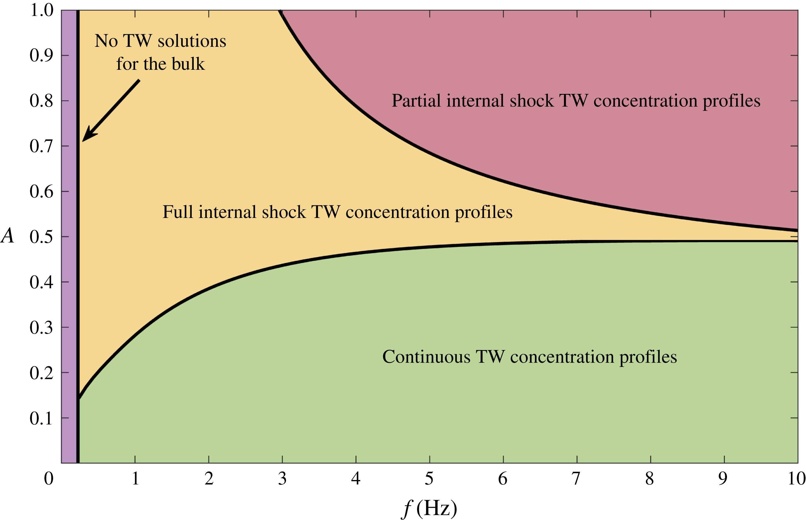
To simulate bidisperse roll waves in an inclined chute, a numerical domain
 $0\leqslant x\leqslant 5~\text{m}$
is discretised over 50 000 grid points, and initial conditions
 $$\begin{eqnarray}\displaystyle h(x,0)=h_{0},\quad \bar{u}(x,0)=\bar{u}_{0},\quad \bar{\unicode[STIX]{x1D719}}(x,0)=\bar{\unicode[STIX]{x1D719}}_{0}, & & \displaystyle\end{eqnarray}$$
representing steady uniform flow are enforced along its length. Note that these conditions do not capture the initial front propagation down the empty chute, but have the advantage of avoiding the degeneracy of the system as
 $h\rightarrow 0$
. The variables at the inflow of the chute are set to be
 $$\begin{eqnarray}\displaystyle h(0,t)=h_{0}+\unicode[STIX]{x1D6FF}h_{1}(t),\quad \bar{u}(0,t)=\bar{u}_{0},\quad \bar{\unicode[STIX]{x1D719}}(0,t)=\bar{\unicode[STIX]{x1D719}}_{0}, & & \displaystyle\end{eqnarray}$$
which constitute the same steady uniform flow as the initial conditions but with a time-dependent perturbation to the flow thickness, designed to trigger the roll wave instability. All simulations are carried out with the same perturbation magnitude
 $\unicode[STIX]{x1D6FF}=h_{0}/100$
, but different forms of the function
 $h_{1}(t)$
are subsequently employed. The numerics are computed using the viscous form of the momentum equation (3.10) with
 $\unicode[STIX]{x1D708}=0.001~\text{m}^{3/2}~\text{s}^{-1}$
.
6.1 Periodic inflow perturbation
The inflow perturbation is initially taken to be a sinusoidal function of the form
 $h_{1}(t)=\sin (2\unicode[STIX]{x03C0}ft)$
, where
 $f=2~\text{Hz}$
is the perturbation frequency. This periodicity is motivated by the desire to produce well-defined regular waves that can be directly related to the ODE travelling-wave solutions derived in §§ 4 and 5.
Numerical simulations showing the thickness
 $h$
(thick solid lines) and interface
 $\unicode[STIX]{x1D702}$
(thin solid lines) profiles at time
 $t=20~\text{s}$
for flows beginning from
 $h_{0}=2~\text{mm}$
and
 $\bar{\unicode[STIX]{x1D719}}_{0}=0.8$
, subject to a periodic inflow perturbation of frequency
 $f=2~\text{Hz}$
. The green shaded region therefore corresponds to the region with large grains and the white region underneath it to small grains. The shear parameter in (a) is
 $A=0.1$
and in (b) is
 $A=0.5$
. Panels (c) and (d) show close ups of the final wave extracted from the PDE solutions (black lines), with the predictions from the inviscid ODE solutions superimposed on top (red lines). Supplementary movies 3 and 4 are available online showing the time evolution of both states.

Figure 12 shows the results of two numerical simulations at time
 $t=20~\text{s}$
, each computed with steady uniform thickness
 $h_{0}=2~\text{mm}$
and concentration
 $\bar{\unicode[STIX]{x1D719}}_{0}=0.8$
. The resulting thickness profiles are thus identical, and the bulk waves grow as they move downslope before their amplitudes eventually saturate (as shown in movies 3 and 4), forming a periodic train of steady travelling waves. Differences in the interface profiles
 $\unicode[STIX]{x1D702}(x,t)$
arise due to different shear parameters
 $A$
being used in the two cases, with figure 12(a) showing a low shear value (
 $A=0.1$
) where the interface largely follows the wave. This corresponds to the ‘continuous’ concentration profiles described in § 5. Figure 12(b), on the other hand, shows a higher shear value (
 $A=0.5$
) which leads to the formation of the second class of solutions with full internal concentration shocks. Numerical simulations have also been carried out in the third regime where
 $h>h_{b}$
everywhere, leading to concentration profiles with partial internal shocks, but these are omitted here for brevity.
These simulations suggest that all classes of travelling-wave solutions predicted by the inviscid ODE are stable and manifest themselves in the full system of viscous PDEs. Figure 12(c,d) extends this idea further by calculating the ODE solutions that have mean total flux
 $q=q_{0}$
and small particle flux
 $q^{S}=q_{0}^{S}$
, and overlaying the profiles on the final downstream wave extracted from the PDE solutions. There is excellent agreement for both the thickness and concentration profiles in both regimes, indicating that solutions of the viscous PDEs are well approximated by inviscid travelling waves. Further comparisons between the inviscid and viscous solutions are described in the Appendix.
To further investigate the kinematics of these two classes of solution, a tracer region of large red particles is now introduced into the simulations, which is designed to mimic the experimental approach of § 2. To achieve this, the mass and momentum balance and transport equations, (3.9), (3.10) and (3.7) are solved as above until
 $t=20~\text{s}$
, allowing a well-developed periodic wavetrain to form. The final thickness, velocity and concentration profiles are then taken as initial conditions for a second set of simulations, where the same equations are solved for
 $h$
,
 $\bar{u}$
and
 $\bar{\unicode[STIX]{x1D719}}$
(with identical inflow perturbation) but an additional transport equation is solved for a new variable, say
 $\bar{\unicode[STIX]{x1D719}}_{R}$
. This represents the relative amount of large red tracer particles, and is governed by the same transport equation (3.7) but with initial and inflow conditions
 $$\begin{eqnarray}\displaystyle & \displaystyle \bar{\unicode[STIX]{x1D719}}_{R}(x,0)=\left\{\begin{array}{@{}ll@{}}\bar{\unicode[STIX]{x1D719}}(x,0) & \text{if}~x_{0}<x<x_{1},\\ 1 & \text{otherwise},\end{array}\right. & \displaystyle\end{eqnarray}$$
 $$\begin{eqnarray}\displaystyle & \displaystyle \bar{\unicode[STIX]{x1D719}}_{R}(0,t)=1, & \displaystyle\end{eqnarray}$$
where
 $x_{0}$
and
 $x_{1}$
are the up- and downslope limits of the tracer region. For a sufficiently narrow range
 $(x_{0},x_{1})$
, solving for
 $\bar{\unicode[STIX]{x1D719}}_{R}$
thus represents the evolving concentration of a (large particle rich) red tracer region, whose boundary is determined by the interface
 $\unicode[STIX]{x1D702}_{R}=h\bar{\unicode[STIX]{x1D719}}_{R}$
. Note that this approach works because the transport equation is decoupled from the bulk, meaning that it can be solved without altering the overall wave properties.
Numerical simulations showing the internal kinematics of the two classes of waves described in figure 12, corresponding to
 $A=0.1$
(a,c,e,g) and
 $A=0.5$
(b,d,f,h). The thick solid lines shows the flow thickness
 $h$
. The green shading indicates large particles, the red shading shows the large red tracer particles and the white region underneath contains small particles. The interfaces between these regions determine the large/small interface
 $\unicode[STIX]{x1D702}$
and the tracer interface
 $\unicode[STIX]{x1D702}_{R}$
. Also shown with red dots are individual surface tracer grains, whose downslope position is calculated using (6.5). Times are given relative to the introduction of the tracer region/particles, and
 $\star$
symbols track a single reference wavefront. Supplementary movies 5 and 6 show an additional representation of the internal kinematics and are available online.

It is also insightful to study the paths of individual tracer particles on the surface of the flow, whose downslope position is determined by
 $$\begin{eqnarray}\displaystyle {\displaystyle \frac{\text{d}x}{\text{d}t}}=u_{s}, & & \displaystyle\end{eqnarray}$$
where the surface velocity
 $u_{s}(x,t)$
is calculated by substituting
 $z=h$
into the shear profile (3.5). Figure 13 and supplementary movies 5 and 6 show the results of these tracer region/particle simulations for the two different shear regimes. In the low shear case (
 $A=0.1$
, figure 13
a,c,e,g and movie 5) the waves always travel faster than the tracer region, consequently catching up and then passing through the red shaded section. A compression/dilation concertina effect is also apparent, with the tracer region quickly being compressed as the wavefront initially passes through and then slowly dilating as it retreats relative to the leeward side of the wave. This is confirmed by the trajectories of surface particles starting at the lateral boundaries of the tracer region
 $x_{0}$
and
 $x_{1}$
. These stay a finite distance apart from each other, but the distance decreases/increases during the wave cycle.
The kinematics of the high shear regime (
 $A=0.5$
, figure 13
b,d,f,h and movie 6) are completely different. In this case a red tracer region starting just behind the wavefront initially travels faster than the waves and is sheared to the front. It then proceeds to travel at precisely the wavespeed, meaning the tracer region remains at the front of the waves for all time. Tracer particles starting from
 $x_{0}$
and
 $x_{1}$
are both sheared to the peak of the wave (where the velocity is fastest) and then continue to move as one and with the travelling wave.
Aerial space–time plots of chute-flow simulations subject to a pseudo-random inflow perturbation, showing a downstream portion of the chute
 $1<x<3.5~\text{m}$
. The green colour shows the evolution of the regular depth-averaged concentration
 $\bar{\unicode[STIX]{x1D719}}$
, and the red colour represents the concentration
 $\bar{\unicode[STIX]{x1D719}}_{R}$
of the tracer region. Mean inflow concentrations are (a)
 $\bar{\unicode[STIX]{x1D719}}_{0}=0.8$
and (b)
 $\bar{\unicode[STIX]{x1D719}}_{0}=0.4$
. Both sets of simulations are conducted using shear parameter
 $A=0.1$
. Supplementary movies 7 and 8 show an additional representation of the internal kinematics and are available online.

6.2 Random inflow perturbation
Experimentally, the red tracer particles dropped on top of the flow travel slower than the waves and exhibit a concertina effect (figure 3), suggesting that the low shear regime is physically appropriate here. Although there is no current experimental evidence for large particles travelling with the wave crests, or faster than the wave crests, it is anticipated that these regimes could exist in more highly sheared flows. Even for the low shear regime, the periodic inflow perturbations described in § 6.1 represent an idealised version of the experiments, which do not form regular wavetrains. To model more realistic flows simulations are now carried out using a pseudo-random inflow perturbation
 $h_{1}(t)$
consisting of a random sum of Fourier modes and coefficients. The regular equations are again solved until
 $t=20~\text{s}$
, before introducing a tracer region near the inflow and tracking its evolution.
Supplementary movies 7 and 8 show the resulting wave and interface profiles, computed using shear parameter
 $A=0.1$
, inflow thickness
 $h_{0}=2~\text{mm}$
and inflow concentrations
 $\bar{\unicode[STIX]{x1D719}}_{0}=0.8$
and
 $\bar{\unicode[STIX]{x1D719}}_{0}=0.4$
corresponding to the two experimental mixtures. The same data are represented as an aerial space–time plot in figure 14 and internal space–time plot in figure 15, which are analogous to the experimental results (figures 3 and 4 respectively). For both mixtures, the random inflow perturbation leads to the development of different waves with varying wavespeeds and amplitudes, some of which merge and coarsen along the length of the chute. From figure 14 it is apparent that large green particles become concentrated at the wave fronts in both cases, but that the waves travel slower in the mixture with more large particles (figure 14
b), consistent with experimental observations. Figure 15 shows that the computed amplitudes are also typically slightly smaller at the end of the chute
 $x=3.25~\text{m}$
for
 $\bar{\unicode[STIX]{x1D719}}_{0}=0.4$
, again in qualitative agreement with experiments. There is, however, still some work necessary to obtain full quantitative agreement, since the amplitude of the computed waves in figure 15(b) is higher than those in the experiments in figure 4(b). There are a number of plausible reasons for this discrepancy. The most likely is that the choice of (i) inflow conditions, (ii) basal friction parameters and (iii) imposed perturbations are not exactly the same as the experiments, resulting in faster growth rates and hence bigger computed waves by the outflow. Certainly, the experimental waves appear still to be growing by the end of the chute, while the computed waves are already quite well developed. There may also be a direct feedback of the local particle size distribution on the bulk flow, which would necessitate fully coupled simulations.
Internal space–time plots corresponding to the random inflow numerical simulations of figure 14 at downslope position
 $x=3.25~\text{m}$
. The thick solid lines represent the flow thickness
 $h$
, the green shading shows the large particle region and the white shaded region beneath is occupied by small particles. The interface
 $\unicode[STIX]{x1D702}$
lies at the transition between these green and white regions. Mean inflow concentrations are (a)
 $\bar{\unicode[STIX]{x1D719}}_{0}=0.8$
and (b)
 $\bar{\unicode[STIX]{x1D719}}_{0}=0.4$
.

Figure 14 and supplementary movies 7 and 8 show that the red tracer region behaves similarly in both cases, moving slower than the waves and experiencing the previously described concertina effect. Note that the time scales are different for the different mixtures in figure 14 because the bulk flow is slower for
 $\bar{\unicode[STIX]{x1D719}}_{0}=0.4$
, meaning that the tracer region gets advected downslope more slowly.
7 Conclusions
This paper presents small-scale experiments in which a mass of bidisperse granular material consisting of large green and small white spherical glass ballotini (
 $200{-}250~\unicode[STIX]{x03BC}\text{m}$
and
 $75{-}150~\unicode[STIX]{x03BC}\text{m}$
diameter, respectively) is released from a hopper and flows down a chute. As the initially homogenous mixture flows over the rough bed, the large particles rise to the free surface due to size segregation. Since the flow is faster near the free surface, the large particles are preferentially transported to the flow front, where a growing region of large particles forms. Upstream of this flow head is a breaking size-segregation wave (Thornton & Gray Reference Thornton and Gray2008; Gray & Ancey Reference Gray and Ancey2009; Johnson et al.
Reference Johnson, Kokelaar, Iverson, Logan, LaHusen and Gray2012), a continuously segregating mixture of large and small grains, which connects the flow head to the inversely graded flow further upstream. The breaking wave ensures that large particles that are over-run by the advancing front are re-segregated upwards into the faster moving layers allowing the large-rich frontal region to grow in size. Small perturbations to the inversely graded upstream flow grow as they travel downslope, eventually developing into fully formed roll waves that travel faster than the bulk flow. These waves have approximately constant velocity (figure 2), although waves exist with a range of wavespeeds, leading to merging events as faster waves engulf slower moving ones. The inversely graded flow, large particle flow head, internal breaking size-segregation wave, and roll waves are directly observed though internal visualisation of the experimental flows (figure 4).
This basic roll wave instability mechanism and subsequent coarsening dynamics are understood for monodisperse flows (Forterre & Pouliquen Reference Forterre and Pouliquen2003; Gray & Edwards Reference Gray and Edwards2014; Razis et al. Reference Razis, Edwards, Gray and van der Weele2014; Edwards & Gray Reference Edwards and Gray2015). In bidisperse flows, there are higher proportions of large particles at the wave fronts compared to the rest of the flow, which consequently form dark green bands in figure 2. Large red tracer particles seeded onto the flow surface travel more slowly than the waves and pass through the wave crests (figure 3), indicating that the increased large particle concentration at the wave fronts is not caused by large particles becoming trapped and accumulating in the wave crests.
Instead, it is caused by spatial variations in the large particle flux in a frame moving with the waves. This results in the layer of large particles on the surface of the flow being compressed in the streamwise direction near the wave crest, and consequently thickening this layer. This compression and thickening is less pronounced in the small particle layer at the base of the flow, meaning that the depth integrated concentration of large particles is increased in the wave crests. This mechanism is observed experimentally; as a wavefront catches up with a region of red tracer particles, these tracers become compressed in the streamwise direction, before dilating after the wave has passed (figure 3).
The formation of bidisperse roll waves and increased concentration of large particles at roll wave crests are predicted by a depth-averaged model for the flow that combines particle size segregation (Gray & Kokelaar Reference Gray and Kokelaar2010a ,Reference Gray and Kokelaar b ) with bulk mass and momentum balance equations (Gray & Edwards Reference Gray and Edwards2014). Motivated by the experimental observations of constant wavespeeds, inviscid travelling-wave solutions are constructed for the bulk thickness and velocity profiles by switching to a moving reference frame. Equating the mean flux of material across one wave with that at the inflow, the model predicts that a given steady uniform flow can develop into a family of different steadily travelling waves, each with different wavespeeds, amplitudes and wavelengths (figure 7). Fixing any one of these properties determines a unique bulk wave profile. Larger-amplitude waves are predicted to travel faster and have longer wavelength (figure 8), which is in agreement with experimental observations of larger-amplitude waves travelling faster than (and consequently merging with) smaller waves. For a given thickness of inflow, mixtures with higher proportions of small particles are predicted to produce waves that travel faster and reach higher amplitudes (figure 8), again consistent with experimental measurements (figure 2).
This agreement occurs despite the fact that frictional differences between large and small particles are accounted for in the model using a basal friction law that depends only on the mean composition of the mixture. The agreement suggests that any increase in the local basal friction caused by increased large particle concentration at wave crests is not central to the formation of roll waves. This is despite such segregation-mobility feedback playing an essential role in other bidisperse flows such as segregation-induced finger formation (Pouliquen et al.
Reference Pouliquen, Delour and Savage1997; Woodhouse et al.
Reference Woodhouse, Thornton, Johnson, Kokelaar and Gray2012; Baker et al.
Reference Baker, Johnson and Gray2016b
). A natural extension to our modelling would be to account for this feedback, by using the local depth-averaged concentration
 $\bar{\unicode[STIX]{x1D719}}(x,t)$
in our friction law (3.13)–(3.16). This coupling adds significant mathematical complexity to the model (since the flow dynamics now depend on the predicted concentration profiles throughout the wave), but is simple to implement in numerical codes, and is likely necessary for quantitative prediction of the dynamics, as well as the kinematics, of bidisperse roll waves.
Having obtained these bulk travelling-wave profiles, travelling-wave solutions can then be constructed for the relative concentration of particles throughout a wave. Three distinct classes of solution are found which all have higher concentrations of large particles towards the front but have key qualitative differences (figure 10). The first ‘continuous’ class of solution has an effective interface between layers of large and small particles that mostly follows the thickness profile, whereas the second ‘full internal shock’ solutions have a region of pure small particles at the rear of the wave transitioning rapidly to a coarser-rich zone at the front across a shock. The third ‘partial internal shock’ solutions are similar to case 2, except that some large particles are present at all points along the wave. By matching the average flux of small particles across a wave to the inflow conditions, one can predict the types of solution that may develop in chute-flow experiments (figure 11). It is found that the continuous concentration profiles typically correspond to low amounts of shear in the flow, the full internal shock solutions occur at higher degrees of shear and the partial internal shock solutions appear for the highest shear values.
Fully time-dependent numerical simulations confirm the existence and stability of the different types of concentration profile solutions (figure 12 and movies 3 and 4), which spontaneously form by perturbing a steady uniform inflow by a known frequency and allowing these perturbations to grow into a well-defined wavetrain. The resulting waves agree extremely well with the theoretical travelling waves, both in terms of the bulk and concentration profiles. The kinematics are also investigated numerically by simulating the evolution of a region of tracer particles, as well as individual grains (figures 13 and 14 and movies 5–8). In the low shear continuous regime, it can be seen that the particles move backwards relative to oncoming waves, and the tracer region dilates and compresses in the same concertina effect observed in the experiments. The kinematics are very different in the higher shear partial and full internal shock regimes, where surface tracer particles either move faster than the waves or move with the velocity of the wavefronts. At the moment there is no experimental evidence of this type of behaviour, but it may well occur in highly sheared geophysical flows.
Irrespective of which type of kinematics dominates, hazardous geophysical mass flows spontaneously develop waves that move significantly faster than depth-averaged flow, have wave peak heights that are significantly higher than an equivalent steady uniform flow and have high concentrations of large particles at their wave crests. All of these factors strongly enhance the impact pressures that such flows can exert on structures in their path, making these flows significantly more destructive than current design criteria may allow for. It is therefore anticipated that modelling roll waves and surges in hazard assessments will become much more important in future.
Acknowledgements
This research was supported by NERC grants NE/E003206/1 and NE/K003011/1 as well as EPSRC grants EP/I019189/1, EP/K00428X/1 and EP/M022447/1. J.M.N.T.G. is a Royal Society Wolfson Research Merit Award holder (WM150058) and an EPSRC Established Career Fellow (EP/M022447/1). J.L.B. would also like to acknowledge support from a NERC doctoral training award and the University of Sydney HPC service. F.M.R. acknowledges financial support from CNPq, Conselho Nacional de Desenvolvimento Científico e Tecnológico – Brazil. All research data supporting this publication are directly available within this publication.
Supplementary movies
Supplementary movies are available at https://doi.org/10.1017/jfm.2018.348.
Appendix A. Construction of viscous travelling-wave solutions
This appendix explains how to construct viscous travelling-wave solutions for the bulk thickness and velocity field, and compares to the analogous inviscid case of § 4. As before, switching to a moving reference frame and seeking steady travelling-wave solutions, the bulk mass and momentum balance (3.9) and (3.10) reduce to
 $$\begin{eqnarray}\displaystyle & \displaystyle {\displaystyle \frac{\text{d}}{\text{d}\unicode[STIX]{x1D709}}}(h(\bar{u}-u_{w}))=0, & \displaystyle\end{eqnarray}$$
 $$\begin{eqnarray}\displaystyle & \displaystyle {\displaystyle \frac{\text{d}}{\text{d}\unicode[STIX]{x1D709}}}(h\bar{u}(\bar{u}-u_{w}))+{\displaystyle \frac{\text{d}}{\text{d}\unicode[STIX]{x1D709}}}\left({\displaystyle \frac{1}{2}}gh^{2}\cos \unicode[STIX]{x1D701}\right)=gh\cos \unicode[STIX]{x1D701}(\tan \unicode[STIX]{x1D701}-\unicode[STIX]{x1D707}_{b})+{\displaystyle \frac{\text{d}}{\text{d}\unicode[STIX]{x1D709}}}\left(\unicode[STIX]{x1D708}h^{3/2}{\displaystyle \frac{\text{d}\bar{u}}{\text{d}\unicode[STIX]{x1D709}}}\right).\quad & \displaystyle\end{eqnarray}$$
Equation (A 1) can be integrated directly to give
 $$\begin{eqnarray}\displaystyle h(u_{w}-\bar{u})=Q_{1}, & & \displaystyle\end{eqnarray}$$
for constant
 $Q_{1}$
, and substituting (A 3) into (A 2) leads to the second-order ODE
 $$\begin{eqnarray}\displaystyle & \displaystyle {\displaystyle \frac{\text{d}^{2}h}{\text{d}\unicode[STIX]{x1D709}^{2}}}=\frac{1}{2h}\left({\displaystyle \frac{\text{d}h}{\text{d}\unicode[STIX]{x1D709}}}\right)^{2}+{\displaystyle \frac{gh^{3/2}\cos \unicode[STIX]{x1D701}}{\unicode[STIX]{x1D708}Q_{1}}}\left[\left(1-{\displaystyle \frac{Q_{1}^{2}}{gh^{3}\cos \unicode[STIX]{x1D701}}}\right){\displaystyle \frac{\text{d}h}{\text{d}\unicode[STIX]{x1D709}}}-\tan \unicode[STIX]{x1D701}+\unicode[STIX]{x1D707}_{b}(h)\right], & \displaystyle\end{eqnarray}$$
with
 $$\begin{eqnarray}\displaystyle & \displaystyle \unicode[STIX]{x1D707}_{b}(h)=\unicode[STIX]{x1D707}_{1}+{\displaystyle \frac{(\unicode[STIX]{x1D707}_{2}-\unicode[STIX]{x1D707}_{1})(hu_{w}-Q_{1})}{\unicode[STIX]{x1D6FE}h^{5/2}+hu_{w}-Q_{1}}}. & \displaystyle\end{eqnarray}$$
Introducing
 $n=\text{d}h/\text{d}\unicode[STIX]{x1D709}$
, allows this to be written as a first-order system
 $$\begin{eqnarray}\displaystyle & \displaystyle {\displaystyle \frac{\text{d}h}{\text{d}\unicode[STIX]{x1D709}}}=n, & \displaystyle\end{eqnarray}$$
 $$\begin{eqnarray}\displaystyle & \displaystyle {\displaystyle \frac{\text{d}n}{\text{d}\unicode[STIX]{x1D709}}}={\displaystyle \frac{1}{2h}}n^{2}+{\displaystyle \frac{gh^{3/2}\cos \unicode[STIX]{x1D701}}{\unicode[STIX]{x1D708}Q_{1}}}\left[\left(1-{\displaystyle \frac{Q_{1}^{2}}{gh^{3}\cos \unicode[STIX]{x1D701}}}\right)n-\tan \unicode[STIX]{x1D701}+\unicode[STIX]{x1D707}_{b}(h)\right], & \displaystyle\end{eqnarray}$$
with unknown parameters
 $u_{w}$
and
 $Q_{1}$
. Gray & Edwards (Reference Gray and Edwards2014) used (A 3) to relate
 $Q_{1}$
to
 $u_{w}$
by assuming that each wave must go through the equilibrium point
 $h=h_{0}$
,
 $\bar{u}=\bar{u}_{0}$
. They then constructed periodic roll wave solutions as limit cycles in
 $(h,n)$
-space around this fixed point by solving an initial value problem (IVP) and extracting the final periodic orbit. Gray & Edwards (Reference Gray and Edwards2014) found that subtly different values of
 $u_{w}$
gave rise to waves with drastically different wavelengths and amplitudes. This approach may be considered as the viscous analogue to the basic solution procedure of § 4.1, with the main difference being that the resulting families of waves no longer travel at exactly the same speed as each other. A slightly different approach is adopted here. The viscous travelling-wave solutions are instead directly related to their parent steady uniform flow, in a similar way to the inviscid case explained in § 4.2. To achieve this, it is useful to define
An example family of viscous roll wave solutions using a BVP solver in (a) the physical plane
 $(\unicode[STIX]{x1D709},h)$
and (b) the phase plane
 $(n,h)$
. Black lines represent previous iterations used to construct the final wave of wavelength 0.3 m (red). The inflow thickness and mean concentration are
 $h_{0}=0.002~\text{m}$
and
 $\bar{\unicode[STIX]{x1D719}}_{0}=0.4$
respectively.

 $$\begin{eqnarray}\displaystyle & \displaystyle m(\unicode[STIX]{x1D709})={\displaystyle \frac{1}{\unicode[STIX]{x1D6EC}}}\int _{0}^{\unicode[STIX]{x1D709}}h(\unicode[STIX]{x1D709}^{\prime })\bar{u}(\unicode[STIX]{x1D709}^{\prime })\,\text{d}\unicode[STIX]{x1D709}^{\prime }, & \displaystyle\end{eqnarray}$$
where
 $\unicode[STIX]{x1D6EC}$
is the wavelength of one wave. Note that
 $m(\unicode[STIX]{x1D6EC})=q$
, with the mean flux
 $q$
being given by (4.24), and hence the waves that form from a steady uniform inflow
 $(h_{0},\bar{u}_{0})$
are those for which
 $m(\unicode[STIX]{x1D6EC})=q_{0}$
. Equation (A 8) can also be written as a first-order ODE (using (A 3))
 $$\begin{eqnarray}\displaystyle & \displaystyle {\displaystyle \frac{\text{d}m}{\text{d}\unicode[STIX]{x1D709}}}={\displaystyle \frac{h}{\unicode[STIX]{x1D6EC}}}\Bigl(u_{w}-{\displaystyle \frac{Q_{1}}{h}}\Bigr), & \displaystyle\end{eqnarray}$$
and the problem can now be reduced to a boundary value problem (BVP) by solving (A 6), (A 7) and (A 9) subject to the boundary conditions
 $$\begin{eqnarray}\displaystyle h(0)=h(\unicode[STIX]{x1D6EC}),\quad n(0)=n(\unicode[STIX]{x1D6EC})=0,\quad m(0)=0,\quad m(\unicode[STIX]{x1D6EC})=q_{0}. & & \displaystyle\end{eqnarray}$$
For a given wavelength
 $\unicode[STIX]{x1D6EC}$
these five conditions allow the two unknown parameters
 $u_{w}$
and
 $Q_{1}$
to be found in conjunction with the three dependent variables
 $h$
,
 $n$
and
 $m$
, providing a suitable initial guess is chosen. Here, such a guess is provided using the solution procedure of Gray & Edwards (Reference Gray and Edwards2014) to find a limit cycle solution, which does not necessarily have the correct average flux or wavelength. The BVP is then solved iteratively, until the solution does have the correct mean flux, using bvp4c in Matlab with the previous solution as an initial guess. At each stage the wavelength is gradually adjusted until it is equal to the required
 $\unicode[STIX]{x1D6EC}$
. Figure 16 shows example wave profiles constructed with this method, with all (black) solutions having the same average flux and the final (red) wave having the desired wavelength.
(a) Comparison between inviscid (solid black lines) and viscous solutions (red dashed lines) of a family of roll wave solutions resulting from a steady uniform inflow thickness
 $h_{0}=2~\text{mm}$
and mean concentration
 $\bar{\unicode[STIX]{x1D719}}_{0}=0.4$
. The dashed black lines represent the theoretical absolute minimum and maximum thickness obtained from the inviscid solution. (b) Close up of the largest wave showing the differences between both solutions.

These viscous travelling-wave solutions can also be directly compared to the inviscid ones constructed in § 4.2. Setting the steady uniform inflow thickness
 $h_{0}$
and mean concentration
 $\bar{\unicode[STIX]{x1D719}}_{0}$
leads to a constant upstream flux
 $q_{0}$
given by equation (4.23). From this inflow flux, a family of inviscid roll waves can be found, each of them having a different amplitude and velocity but all with the same flux as
 $q_{0}$
(illustrated in figure 7). The wavelength of each of these inviscid waves can then be matched by the BVP procedure described above to get the corresponding viscous solution. Figure 17(a) shows a comparison between inviscid and viscous travelling waves for the same inflow flux (
 $h_{0}=0.002~\text{m}$
and
 $\bar{\unicode[STIX]{x1D719}}_{0}=0.4$
). The viscous solution is almost identical to the inviscid one and a close-up view is actually needed to see any influence of the viscosity on the wave properties. In figure 17(b), a zoom of the last wave shows the difference between both solutions. As expected, the viscosity smooths the shape of the wave and leads to a less sharp shock, but the differences are otherwise minimal.


 Open access

