





1. Introduction
Meticulous understanding of plasma turbulence is essential for explaining different nonlinear phenomena in space and astrophysics. At length scales larger than the ion inertial length (
 $d_i$
), plasma behaviour is described by magnetohydrodynamics (MHD), in which the dynamics of an ion–electron plasma is effectively captured by the centre-of-mass fluid. In the limit of infinite conductivity, the magnetic field lines are frozen to the MHD fluid. However, for length scales comparable or inferior to
 $d_i$
but superior to the electron inertial scale (
 $d_e$
), the ion and electron fluids no longer move together and the magnetic field lines are frozen only in the electron fluid. At those scales, one has to consider a Hall MHD (HMHD) model where the induction equation is given by
 \begin{equation} \partial _t {\boldsymbol{b}} - \eta {\nabla} ^2 {{\boldsymbol{b}}} =\boldsymbol{\nabla }\times ({\boldsymbol{u}}\times {\boldsymbol{b}})- d_i \boldsymbol{\nabla }\times ({\boldsymbol{j}}\times {\boldsymbol{b}}), \end{equation}
where
 $\boldsymbol{u}$
is the velocity of the centre-of-mass fluid,
 $\boldsymbol{b}$
is the magnetic field expressed in Alfvén units,
 $\eta$
is the magnetic diffusivity,
 ${\boldsymbol{j}}=\boldsymbol{\nabla }\times {\boldsymbol{b}}$
represents the current and the last term on the right-hand side represents the Hall term. The presence of the Hall term distinguishes a HMHD flow from an ordinary MHD flow both in terms of the linear wave modes and turbulence. An ordinary incompressible MHD flow responds to a weak perturbation in terms of non-dispersive Alfvén waves, whereas the inclusion of the Hall term induces dispersion which mostly acts at scales comparable to or smaller than
 $d_i$
. For length scales much larger than
 $d_i$
, one recovers the Alfvén waves. However, at scales much smaller than
 $d_i$
, the dispersion relation splits into right-circularly polarised whistler and left-circularly polarised ion-cyclotron waves (Lighthill Reference Lighthill1960; Galtier Reference Galtier2016). Beyond the linear regime, HMHD turbulence distinguishes itself by the formation of fine-scale current sheets and tubular structures (Miura Reference Miura2024). However, similar to MHD, the total energy
 $(\int (u^2+b^2)/2\ {\rm d}\tau )$
is also an inviscid invariant of HMHD, where
 $\text{d}\tau$
represents the elementary volume element. In fully developed HMHD turbulence, one therefore expects a universal energy cascade with constant flux rate
 $\varepsilon$
across the extended inertial range comprising both MHD and Hall dominated sub-ion scales. In the realm of space and astrophysical plasmas, the cascade rate
 $\varepsilon$
is pivotal to unravelling the mechanisms behind magnetic reconnection (Huba & Rudakov Reference Huba and Rudakov2004; Drake, Shay & Swisdak Reference Drake, Shay and Swisdak2008; Sullivan, Bhattacharjee & Huang Reference Sullivan, Bhattacharjee and Huang2009; Huang, Bhattacharjee & Sullivan Reference Huang, Bhattacharjee and Sullivan2011), turbulent heating (Sorriso-Valvo et al. Reference Sorriso-Valvo, Marino, Carbone, Noullez, Lepreti, Veltri, Bruno, Bavassano and Pietropaolo2007; Sahraoui et al. Reference Sahraoui, Goldstein, Robert and Khotyaintsev2009; Marino & Sorriso-Valvo Reference Marino and Sorriso-Valvo2023), small-scale dynamos (Mininni et al. Reference Mininni, Gomez and Mahajan2003, Reference Mininni, Alexakis and Pouquet2007; Kumar, Verma & Samtaney Reference Kumar, Verma and Samtaney2013) etc. The analytical expressions of
 $\varepsilon$
, obtained from exact relations in terms of two-point correlators or increments of relevant flow variables such as the velocity, the magnetic field etc. (Politano & Pouquet Reference Politano and Pouquet1998; Galtier Reference Galtier2008; Banerjee & Galtier Reference Banerjee and Galtier2013; Banerjee & Kritsuk Reference Banerjee and Kritsuk2017; Andrés et al. Reference Andrés, Galtier and Sahraoui2018; Banerjee & Kritsuk Reference Banerjee and Kritsuk2018; Andrés & Banerjee Reference Andrés and Banerjee2019), are indeed used to calculate the turbulent heating rate using both numerical and observational data of plasma turbulence (Hellinger et al. Reference Hellinger, Verdini, Landi, Franci and Matteini2018; Andrés et al. Reference Andrés, Sahraoui, Galtier, Hadid, Ferrand and Huang2019; Ferrand et al. Reference Ferrand, Galtier, Sahraoui, Meyrand, Andrés and Banerjee2019; Bandyopadhyay et al. Reference Bandyopadhyay2020). Interestingly, in Fourier space, the energy transfer induced by the Hall term is found to differ significantly from that of ordinary MHD. At MHD scales, the magnetic energy spectrum follows a Kolmogorov-like
 $k^{-5/3}$
power law whereas a
 $k^{-7/3}$
spectrum emerges beyond the ion inertial scale (Krishan & Mahajan Reference Krishan and Mahajan2004a
,
Reference Krishan and Mahajanb
; Miura, Yang & Gotoh Reference Miura, Yang and Gotoh2019), where
 $k$
is the wavenumber. In addition, when
 $k$
is less than the Hall wavenumber
 $k_H (\sim d_i^{-1})$
, the modal transfer rate of magnetic energy due to the Hall term becomes negative, leading to a backscatter of magnetic energy to the large scales (Mininni, Alexakis & Pouquet Reference Mininni, Alexakis and Pouquet2007; Gómez et al. Reference Gómez, Mininni and Dmitruk2010). To investigate the distinct nature of the energy transfers between MHD and HMHD in depth, it is customary to analyse in terms of the resonating energy conserving wavevector triads
 $({\boldsymbol{k}},{\boldsymbol{p}},{\boldsymbol{q}})$
such that
 ${\boldsymbol{k}} + {\boldsymbol{p}} +{\boldsymbol{q}} = \boldsymbol{0}$
. The triads are said to be local if
 $k\simeq p\simeq q$
whereas for non-local triads we have one of the sides being significantly smaller or larger than the other two sides (note that a side of the triangle can be arbitrarily small with respect to the other two sides, whereas it cannot be arbitrarily larger than the other two as mandated by the law of cosines). On the other hand, the energy transfer is said to be local when the giver and the receiver modes are closely situated while the mediator mode, in principle, may be located anywhere. A local triad therefore always leads to local transfer whereas a non-local triad may associate a local or non-local transfer according to whether the giver and the receiver modes are of comparable sizes or not, respectively. Apart from small non-local transfers due to the energy-containing large-scale structures in MHD (Alexakis, Mininni & Pouquet Reference Alexakis, Mininni and Pouquet2005; Carati et al. Reference Carati, Debliquy, Knaepen, Teaca and Verma2006; Cho Reference Cho2010), the inertial-scale energy transfers in both hydrodynamics (HD) and MHD turbulence are predominantly mediated by the local triads (Kraichnan Reference Kraichnan1971; Verma, Ayyer & Chandra Reference Verma, Ayyer and Chandra2005). For HMHD turbulence, the situation becomes trickier. Whereas the total energy transfer remains local in nature, the energy transfer due to the Hall term shows clear signatures of non-locality in the modal transfer of magnetic energy (Mininni et al. Reference Mininni, Alexakis and Pouquet2007; Gómez et al. Reference Gómez, Mininni and Dmitruk2010; Araki & Miura Reference Araki and Miura2011). Despite these studies, a dedicated study to investigate the possible source of such non-locality is still awaited. Also in those studies, the energy transfer was simply interpreted as an exchange between different modes of the
 $\boldsymbol{b}$
-fields only. However,
 $\boldsymbol{b}$
and
 $\boldsymbol{j}$
are connected with each other through space and time coordinates but one is not an explicit closed form of the other in the physical space. Whether all sorts of exchange due to the Hall term can be attributed to the
 $\boldsymbol{b}$
-field is a matter of debate. The total Hall term looks very similar to
 $\boldsymbol{\nabla }\times ({\boldsymbol{u}}\times {\boldsymbol{b}})$
, which is the nonlinear term in the induction of ordinary MHD. Albeit non-unique, one can be inspired by the
 $\boldsymbol{u}$
-to-
 $\boldsymbol{b}$
and
 $\boldsymbol{b}$
-to-
 $\boldsymbol{b}$
decomposition in ordinary MHD (Plunian, Stepanov & Verma Reference Plunian, Stepanov and Verma2019) and decompose the Hall term into two parts as
 $\boldsymbol{\nabla }\times ({\boldsymbol{j}}\times {\boldsymbol{b}} )=- ({\boldsymbol{j}}\boldsymbol{\cdot }\boldsymbol{\nabla } ){\boldsymbol{b}} + ({\boldsymbol{b}}\boldsymbol{\cdot }\boldsymbol{\nabla }){\boldsymbol{j}}$
to compare their individual contributions in the energy transfer.Footnote
1
The channel corresponding to
 $- ({\boldsymbol{j}}\boldsymbol{\cdot }\boldsymbol{\nabla }){\boldsymbol{b}}$
is labelled as channel
 $\mathcal{BB}$
and the channel corresponding to
 $({\boldsymbol{b}}\boldsymbol{\cdot }\boldsymbol{\nabla }){\boldsymbol{j}}$
is labelled as channel
 $\mathcal{JB}$
. In fact, rather than
 $\boldsymbol{j}$
, here, the variable of interest is
 $-d_i{\boldsymbol{j}}$
, which is the relative velocity between electron and the ion fluids which essentially reduces to the electron fluid velocity in the small-scale limit
 $(kd_i\gg 1)$
, where the motion of the ions can be neglected (Biskamp et al. Reference Biskamp, Schwarz, Zeiler, Celani and Drake1999).
Note that this decomposition has already been used to explore the small-scale dynamo action and the mode-to-mode transfer rates due to the Hall term (Halder et al. Reference Halder, Banerjee, Chatterjee and Sharma2023; Banerjee & Halder Reference Banerjee and Halder2024). By rigorous calculation, it was shown that the magnetic energy transfers through
 $\mathcal{BB}$
and
 $\mathcal{JB}$
channels are separately conserved in each triad
 ${\boldsymbol{k}} + {\boldsymbol{p}} +{\boldsymbol{q}} =\boldsymbol{0}$
. However, the nature of triadic conservation for the two channels is found to be structurally different (Banerjee & Halder Reference Banerjee and Halder2024). The transfers through the channel
 $\mathcal{BB}$
are made up of three fundamental transfer unitsFootnote
2
whereas the transfers of the channel
 $\mathcal{JB}$
consist of five fundamental units. In addition, for the small-scale HMHD dynamos, the channel
 $\mathcal{JB}$
is found to be the primary contributor to the small-scale turbulent Hall dynamo (Halder et al. Reference Halder, Banerjee, Chatterjee and Sharma2023). These aspects motivate a study to explore the direction and locality of energy transfer corresponding to each of the two channels.
In this paper, using direct numerical simulations of HMHD turbulence with
 $512^3$
grid points, we thoroughly examine the locality (or non-locality) of magnetic energy transfer through the aforesaid two channels. Employing shell-to-shell (S2S hereinafter) transfer rates, we calculate the local and non-local contributions originating from each term, and identify the direct or inverse character of the resulting transfer. While both of the channels contain the signature of back transfer to large scales, their scale-wise behaviours are found to differ significantly from each other. In particular, for the channel
 $\mathcal{JB}$
, a change of nature of the local transfer is observed across the Hall wavenumber
 $k_H$
. To further characterise the locality of the triads, we compute S2S transfer rates for a fixed giver shell (denoted as the mediator-specific transfer later) and find a prominent disparity between the two channels. Finally, assuming a heuristic power-law behaviour of the modal fields, we propose some quantitative comparison on the basis of our observed results.
The paper is organised as follows: in § 2, we present the governing equations, the definition of the energy transfer rates and discuss the numerical methods along with the simulation details. Section 3 consists of the calculation of the flux and S2S transfer rates with and without fixing the giver shell together with a heuristic quantitative interpretation of our findings. Finally, in § 4, we summarise and conclude.
2. Methodology
2.1. Governing equations and energy transfer rates
The inviscid incompressible HMHD equations are given by
 \begin{align} \partial _t {\boldsymbol{u}} &= -({\boldsymbol{u}}\boldsymbol{\cdot }\boldsymbol{\nabla }){\boldsymbol{u}} + ({\boldsymbol{b}}\boldsymbol{\cdot }\boldsymbol{\nabla }){\boldsymbol{b}} -\boldsymbol{\nabla } P_T ,\\[-10pt]\nonumber \end{align}
 \begin{align} \partial _t {\boldsymbol{b}} &=-({\boldsymbol{u}}\boldsymbol{\cdot }\boldsymbol{\nabla }){\boldsymbol{b}} +({\boldsymbol{b}}\boldsymbol{\cdot }\boldsymbol{\nabla }){\boldsymbol{u}}+ d_i\left ({\boldsymbol{j}}\boldsymbol{\cdot }\boldsymbol{\nabla }\right ){\boldsymbol{b}} -d_i\left ({\boldsymbol{b}}\boldsymbol{\cdot }\boldsymbol{\nabla }\right ){\boldsymbol{j}},\\[-10pt]\nonumber \end{align}
 \begin{align} &\boldsymbol{\nabla } \boldsymbol{\cdot }{\boldsymbol{u}} = 0, \;\; \boldsymbol{\nabla } \boldsymbol{\cdot }{\boldsymbol{b}} = 0, \end{align}
where
 $P_T = p+b^2/2$
is the total pressure. To examine the locality of the energy conserving triads, it is customary to obtain the evolution equations for
 $n$
th-shell energy densities
 $E^u_n$
and
 $E^b_n$
as
 \begin{align} \partial _t E^u_n &= \sum _m\partial _t E^u_{n, m} =\sum _m \left [T^{u, u}_{n, m} + T^{u, b}_{n, m}\right ]\!,\\[-10pt]\nonumber \end{align}
 \begin{align} \partial _t E^b_n &= \sum _m\partial _t E^b_{n, m} =\sum _m \left [ T^{b, b}_{n, m} + T^{b, u}_{n, m} + \mathcal{H}^{b, b}_{n, m} + \mathcal{H}^{b, j}_{n, m}\right ]\!, \end{align}
where
 $E^u_n =\sum _{|{\boldsymbol{k}}|\in n}{\boldsymbol{u}}_{{\boldsymbol{k}}}\boldsymbol{\cdot }{\boldsymbol{u}}_{{\boldsymbol{k}}}^* /2$
and
 $E^b_n =\sum _{|{\boldsymbol{k}}|\in n}{\boldsymbol{b}}_{{\boldsymbol{k}}}\boldsymbol{\cdot }{\boldsymbol{b}}_{{\boldsymbol{k}}}^* /2$
, with
 ${\boldsymbol{u}}_{{\boldsymbol{k}}}$
and
 ${\boldsymbol{b}}_{{\boldsymbol{k}}}$
denoting the Fourier transforms of
 ${\boldsymbol{u}}(\boldsymbol{x})$
and
 ${\boldsymbol{b}}(\boldsymbol{x})$
, respectively, and where
 $T^{x, y}_{n, m}$
represents the net transfer rate in ordinary MHD from the field
 ${\boldsymbol{y}}_{\kern-2pt{\boldsymbol{p}}}$
to the field
 ${\boldsymbol{x}}_{{\boldsymbol{k}}}$
, where
 $\left |{\boldsymbol{p}}\right |$
and
 $\left |{\boldsymbol{k}}\right |$
belong to the shells
 $m$
and
 $n$
, respectively, and is mathematically expressed as
 \begin{equation} T^{x, y}_{n, m}= {\mathscr{S}} ({\boldsymbol{x}}, {\boldsymbol{y}}) \sum _{|{\boldsymbol{k}}|\in n}\sum _{|{\boldsymbol{p}}|\in m}^{\varDelta }\Im [({\boldsymbol{p}}\boldsymbol{\cdot }{\boldsymbol{z}}_{{\boldsymbol{q}}})({\boldsymbol{y}}_{\kern-2pt{\boldsymbol{p}}}\boldsymbol{\cdot }{\boldsymbol{x}}_{{\boldsymbol{k}}})] ,\end{equation}
where
 $\boldsymbol{x}$
,
 $\boldsymbol{y}$
and
 $\boldsymbol{z}$
can be
 $\boldsymbol{u}$
and
 $\boldsymbol{b}$
with
 $\Im$
denoting the imaginary part of a complex number,
 ${\mathscr{S}} ({\boldsymbol{x}}, {\boldsymbol{y}}) = 1$
if
 $\boldsymbol{x}$
and
 $\boldsymbol{y}$
represent the same field and is equal to
 $-1$
otherwise and
 $\varDelta$
denotes the condition
 ${\boldsymbol{k}}+{\boldsymbol{p}}+{\boldsymbol{q}}=\boldsymbol{0}$
. The terms
 $\mathcal{H}^{b, b}_{n, m}$
and
 $\mathcal{H}^{b, j}_{n, m}$
represent the S2S transfer rates due to the Hall term and are defined below. In the present context, the quantity
 $\Im [({\boldsymbol{p}}\boldsymbol{\cdot }{\boldsymbol{z}}_{{\boldsymbol{q}}})({\boldsymbol{y}}_{\kern-2pt{\boldsymbol{p}}}\boldsymbol{\cdot }{\boldsymbol{x}}_{{\boldsymbol{k}}})]$
represents the field specific mode-to-mode transfer rate from
 ${\boldsymbol{y}}_{\kern-2pt{\boldsymbol{p}}}$
to
 ${\boldsymbol{x}}_{{\boldsymbol{k}}}$
, with
 $\boldsymbol{k}$
,
 $\boldsymbol{p}$
and
 $\boldsymbol{q}$
being denoted as the receiver, giver and mediator wave modes, respectively (Dar, Verma & Eswaran Reference Dar, Verma and Eswaran2001; Verma Reference Verma2004; Banerjee & Halder Reference Banerjee and Halder2024). Note that, these transfer rates are defined without symmetrising the triads and the definitions of giver and mediators are debatable. However, previous works have shown that S2S transfer rates can be properly defined (i.e. they conserve energy and have all properties expected for a transfer function), and calculated much more easily if one uses the non-symmetrised expressions (Dar et al. Reference Dar, Verma and Eswaran2001; Teimurazov et al. Reference Teimurazov, Stepanov, Verma, Barman, Kumar and Sadhukhan2018). Nonetheless, it is important to recognise that a phenomenological interpretation based on the concepts of the giver and mediator wavenumbers constitutes just one of several plausible interpretations. Similar to the aforementioned nonlinear transfers,
 $\mathcal{H}^{b, b}_{n, m}$
and
 $\mathcal{H}^{b, j}_{n, m}$
represent the transfer rates associated with
 $d_i ({\boldsymbol{j}}\boldsymbol{\cdot }\boldsymbol{\nabla } ){\boldsymbol{b}}$
and
 $-d_i ({\boldsymbol{b}}\boldsymbol{\cdot }\boldsymbol{\nabla } ){\boldsymbol{j}}$
, respectively and are written as
 \begin{align} \mathcal{H}^{b, b}_{n, m}&=-d_i\sum _{|{\boldsymbol{k}}|\in n}\sum _{|{\boldsymbol{p}}|\in m}^{\varDelta }\Im \left [\left ({\boldsymbol{p}}\boldsymbol{\cdot }{\boldsymbol{j}}_{{\boldsymbol{q}}}\right )\left ({\boldsymbol{b}}_{\kern-1pt{\boldsymbol{p}}}\boldsymbol{\cdot }{\boldsymbol{b}}_{{\boldsymbol{k}}}\right )\right ]\!, \end{align}
 \begin{align} \mathcal{H}^{b, j}_{n, m}&=d_i\sum _{|{\boldsymbol{k}}|\in n}\sum _{|{\boldsymbol{p}}|\in m}^{\varDelta }\Im \left [\left ({\boldsymbol{p}}\boldsymbol{\cdot }{\boldsymbol{b}}_{{\boldsymbol{q}}}\right )\left ({\boldsymbol{j}}_{\kern-1.5pt{\boldsymbol{p}}}\boldsymbol{\cdot }{\boldsymbol{b}}_{{\boldsymbol{k}}}\right )\right ]\!. \end{align}
Following the standard nomenclature of mode-to-mode transfers, it is straightforward to recognise that the transfers in (2.7) and (2.8) are associated with the channels
 $\mathcal{BB}$
and
 $\mathcal{JB}$
, respectively. In HMHD, however, no term of energy transfer is obtained by taking the scalar product of the HMHD equations with
 $\boldsymbol{j}$
and hence the back transfer for the channel
 $\mathcal{JB}$
does not appear. In the shell picture, the transfer is said to be local if the shell number
 $n$
mostly receives energy from the neighbouring shells whereas for the non-local transfers a non-negligible contribution also comes from the distant shells.
2.2. Numerical details
Simulation parameters. Here,
 $N^3$
is the number of grid points,
 $\nu _h$
is the hyperviscous coefficient,
 $\eta _h$
is the hyperdiffusive coefficient,
 $d_i$
is the ion inertial length,
 $f_0$
is the external forcing amplitude and
 $k_{d}$
is the hyperviscous Kolmogorov wavenumber.

Table 1. Long description
The table presents simulation parameters used in a study on turbulence. It contains one row and seven columns. The columns are labeled as follows: N, vh = ηh, di, f0, kd, kmax/kd. The row provides the following values: 512, 10^-7, 0.05, 0.5, 100, 1.7. The table summarizes key parameters including the number of grid points, hyperviscous coefficient, hyperdiffusive coefficient, ion inertial length, external forcing amplitude, and hyperviscous Kolmogorov wavenumber.
(a) Instantaneous slice of absolute values of magnetic and current fields at statistical steady state. Both fields show signature of a fully developed turbulent flow. (b) Kinetic and magnetic energy spectra at steady state as a function of wavenumber
 $k$
. The dashed vertical line represents the Hall wavenumber
 $k_H$
.

We solve (2.1) and (2.2) using a parallel pseudo-spectral code in a three-dimensional periodic domain with
 $512^3$
grid points. The box length is taken to be
 $2\pi$
in each spatial direction. In our simulation, we take
 $d_i =0.05$
below which the Hall effect is expected to be visible. The aliasing error is removed with the standard 2/3-dealiasing method which fixes the maximum available wavenumber
 $k_{max}\approx 171$
(Orszag Reference Orszag1971). A fourth-order Runge–Kutta scheme is used for time integration and the time step is adjusted with the Courant-Friedrichs-Lewy condition. The turbulence is generated and sustained by Taylor–Green forcing
 $\boldsymbol{f}= f_0 [\sin(k_0x)\cos(k_0y)\cos(k_0z),$
 $-\cos(k_0x)\sin(k_0y)\cos(k_0z)]$
with
 $f_0 = 0.5$
and
 $k_0=2$
, which corresponds to the forcing wavenumber
 $k_f = k_0\sqrt {3}\approx 3.4$
. A clear inertial range can be obtained if the dissipative terms contain higher-order derivatives as compared with the nonlinear terms. In order to avoid the contamination of Hall contribution due to the usual dissipative effects
 $({\sim}{\nabla} ^2)$
, here we employ a
 ${\nabla} ^4$
-hyperdiffusive operator in both the momentum and induction equations. Note that the magnetic Prandtl number for our simulation is taken to be unity. The simulation is well resolved as the ratio
 $k_{max}/k_d \gt 1$
, where
 $k_d = (\varepsilon /\nu _h^3)^{(1/10)}$
is the hyperviscous Kolmogorov wavenumber, where
 $\varepsilon$
is the total dissipation rate and
 $\nu _h$
is the hyperviscous coefficient (Banerjee, Halder & Das Reference Banerjee, Halder and Das2025). The relevant simulation parameters are summarised in table 1. All of the numerical calculations are performed when the system reaches a statistical steady state balancing the average injection and dissipation of total energy. An instantaneous slice of the magnetic and current fields (see figure 1
a) shows the clear signature of fully developed homogeneous turbulence. In figure 1(b), we plot the power spectra for magnetic and kinetic energies as a function of wavenumber
 $k$
. For scales larger than the
 $d_i$
, magnetic and kinetic energies follow
 $k^{-1.3}$
and
 $k^{-1.2}$
, respectively, whereas for scales below
 $d_i$
, the magnetic and the kinetic energy spectra follow
 $k^{-7/3}$
and
 $k^{-5/3}$
power laws, respectively. The spectra for scales larger than
 $d_i$
are shallower than the ones reported in earlier studies on HMHD turbulence (Miura et al. Reference Miura, Yang and Gotoh2019; Yadav, Miura & Pandit Reference Yadav, Miura and Pandit2022). In our simulations with
 $512^3$
grid points, the forcing wavenumber
 $k_f \approx 3.4$
and the Hall wavenumber
 $k_H\approx 20$
are close and hence a well-separated MHD inertial range is not obtained. However, an extended inertial range with kinetic and magnetic spectral exponents close to
 $-1.5$
and
 $-1.6$
is obtained for a simulation with
 $512^3$
grid points and
 $d_i = 0.02$
, corresponding to
 $k_H \approx 50$
(see figure 9
a in § 3.5). Nevertheless, we continue using
 $k_H = 20$
throughout the entire analysis in order to keep the Hall wavenumber approximately in the middle of the logarithmic wavenumber range (see figure 1
a). One may then question the robustness of the results as
 $k_H$
changes. To verify that, we have explicitly calculated the S2S transfer rates and show that the main conclusion regarding the nature of energy transfer in the two channels remains unchanged (see figures 10
a and 10
b in § 3.5).
To capture a clear picture of the energy transfer in the inertial range, we construct
 $25$
concentric shells with the radii:
 $k_n\in \{0, 2, 4, 8, \ldots , 128, 256\}$
where the radii between
 $8$
and
 $128$
are logarithmically binned with the ratio
 $k_n/k_{n-1}=1.15$
, between the subsequent shells. Note that, in our case, the inner and outer radii of the
 $n$
th shell are
 $k_{n-1}$
and
 $k_{n}$
, respectively. The choice of logarithmic binning for the intermediate wavenumbers is adopted to ensure localisation of small turbulent eddies in the physical space (Eyink & Aluie Reference Eyink and Aluie2009). This is due to the fact that shell thickness grows with increasing radius, enabling the accumulation of a large number of Fourier modes in the high wavenumber region. In contrast, linear binning generates shells of uniform thickness, which does not necessarily guarantee such localisation (see Appendix A). Using the aforementioned radii, we also calculate the corresponding flux rates for the kinetic energy and the magnetic energy (MHD and Hall contributions), in addition to the total energy injection and the dissipation rates as
 \begin{align} \varPi _u (k_0) =& -\sum _{|{\boldsymbol{k}}|\leqslant k_0} \sum _{|{\boldsymbol{p}}|\gt k_0}^{\varDelta }\Im [ ({\boldsymbol{p}}\boldsymbol{\cdot }{\boldsymbol{u}}_{{\boldsymbol{q}}})({\boldsymbol{u}}_{{\boldsymbol{p}}}\boldsymbol{\cdot }{\boldsymbol{u}}_{{\boldsymbol{k}}})-({\boldsymbol{p}}\boldsymbol{\cdot }{\boldsymbol{b}}_{{\boldsymbol{q}}})({\boldsymbol{b}}_{\kern-1pt{\boldsymbol{p}}}\boldsymbol{\cdot }{\boldsymbol{u}}_{{\boldsymbol{k}}})],\\[-10pt]\nonumber \end{align}
 \begin{align} \varPi _b (k_0) =& - \sum _{|{\boldsymbol{k}}|\leqslant k_0}\sum _{|{\boldsymbol{p}}|\gt k_0}^{\varDelta } \Im [ ({\boldsymbol{p}}\boldsymbol{\cdot }{\boldsymbol{u}}_{{\boldsymbol{q}}})({\boldsymbol{b}}_{\kern-1pt{\boldsymbol{p}}}\boldsymbol{\cdot }{\boldsymbol{b}}_{{\boldsymbol{k}}})-({\boldsymbol{p}}\boldsymbol{\cdot }{\boldsymbol{b}}_{{\boldsymbol{q}}})({\boldsymbol{u}}_{{\boldsymbol{p}}}\boldsymbol{\cdot }{\boldsymbol{b}}_{{\boldsymbol{k}}})],\\[-10pt]\nonumber \end{align}
 \begin{align} \varPi _{Hall} (k_0) =& -d_i \sum _{|{\boldsymbol{k}}|\leqslant k_0}\sum _{|{\boldsymbol{p}}|\gt k_0}^{\varDelta } \Im [ ({\boldsymbol{p}}\boldsymbol{\cdot }{\boldsymbol{b}}_{{\boldsymbol{q}}})({\boldsymbol{j}}_{\kern-1.5pt{\boldsymbol{p}}}\boldsymbol{\cdot }{\boldsymbol{b}}_{{\boldsymbol{k}}})-({\boldsymbol{p}}\boldsymbol{\cdot }{\boldsymbol{j}}_{{\boldsymbol{q}}})({\boldsymbol{b}}_{\kern-1pt{\boldsymbol{p}}}\boldsymbol{\cdot }{\boldsymbol{b}}_{{\boldsymbol{k}}})]\nonumber \\ & - d_i \sum _{|{\boldsymbol{k}}|\leqslant k_0}\sum _{|{\boldsymbol{p}}|\leqslant k_0}^{\varDelta }\Im [ ({\boldsymbol{p}}\boldsymbol{\cdot }{\boldsymbol{b}}_{{\boldsymbol{q}}})({\boldsymbol{j}}_{\kern-1.5pt{\boldsymbol{p}}}\boldsymbol{\cdot }{\boldsymbol{b}}_{{\boldsymbol{k}}})],\\[-10pt]\nonumber \end{align}
 \begin{align} \varPi _{inj} (k_0) =& \sum _{|{\boldsymbol{p}}|\leqslant k_0} \Re \big[{\boldsymbol{u}}_{{\boldsymbol{p}}}^*\boldsymbol{\cdot }\boldsymbol{f}_{\kern-2.6pt{\boldsymbol{p}}}\big]\;\; \text{and}\\[-10pt]\nonumber \end{align}
 \begin{align} \varPi _{D} (k_0) =& -\sum _{|{\boldsymbol{p}}|\leqslant k_0} \left [ \nu _h p^{4} |{\boldsymbol{u}}_{{\boldsymbol{p}}}^*|^2 + \eta _h p^{4} |{\boldsymbol{b}}_{\kern-1pt{\boldsymbol{p}}}^*|^2 \right ]\!, \end{align}
respectively.Footnote 3
It is interesting to note that the term
 $- d_i \sum _{|{\boldsymbol{k}}|\leqslant k_0}\sum _{|{\boldsymbol{p}}|\leqslant k_0}^{\varDelta }\Im [ ({\boldsymbol{p}}\boldsymbol{\cdot }{\boldsymbol{b}}_{{\boldsymbol{q}}})({\boldsymbol{j}}_{\kern-1.5pt{\boldsymbol{p}}}\boldsymbol{\cdot }{\boldsymbol{b}}_{{\boldsymbol{k}}})]$
in (2.11) represents the net transfer rate of magnetic energy with both
 $|{\boldsymbol{p}}|$
and
 $|{\boldsymbol{k}}|$
being inside a sphere of radius
 $k_0$
. For transfer of energy from
 $\boldsymbol{x}$
-to-
 $\boldsymbol{y}$
field, this particular term gets cancelled with a similar type of contribution emerging from the corresponding back transfer from
 $\boldsymbol{y}$
-to-
 $\boldsymbol{x}$
. This is true for
 $\boldsymbol{u}$
-to-
 $\boldsymbol{u}$
,
 $\boldsymbol{b}$
-to-
 $\boldsymbol{b}$
and
 $\boldsymbol{b}$
-to-
 $\boldsymbol{u}$
transfers where the corresponding back transfers automatically exist for the first two cases and also holds for the third case where
 $\boldsymbol{u}$
-to-
 $\boldsymbol{b}$
transfers participate in the resulting energy cascade (Verma Reference Verma2019; Banerjee & Halder Reference Banerjee and Halder2024). In the case of HMHD, the energy transfer involves channels
 $\mathcal{BB}$
and
 $\mathcal{JB}$
where the back transfer for the channel
 $\mathcal{JB}$
does not appear in the energy transfer. The aforementioned contribution is therefore not counter-balanced and survives in the calculation of
 $\varPi _{Hall}$
(see Appendix B).
(a) Total energy flux rates, with and without the contribution from the Hall term, as a function of wavenumber
 $k$
;
 $\varPi _{inj}$
and
 $\varPi _{D}$
respectively denote the flux rates due to injection and total energy dissipation. (b) Various components of the total flux as function of wavenumber
 $k$
. Here,
 $\varPi _{b}$
,
 $\varPi _{u}$
and
 $\varPi _{Hall}$
respectively denote flux rates for magnetic, kinetic energies and due to the Hall term with
 $\varPi _{Total} = \varPi _{b}+\varPi _{u}+\varPi _{Hall}$
.

Figure 2. Long description
Two line graphs depict the energy flux rates and their components as functions of wavenumber. Panel A: The line graph shows the total energy flux rates with and without the contribution from the Hall term as a function of wavenumber. The x-axis represents the wavenumber on a logarithmic scale, and the y-axis represents the flux rates on a logarithmic scale. The graph includes multiple lines representing different flux rates, such as the total energy flux rate, the flux rate without the Hall term, the flux rate due to injection, and the total energy dissipation rate. Panel B: The line graph shows various components of the total flux as a function of wavenumber. The x-axis represents the wavenumber on a logarithmic scale, and the y-axis represents the flux rates. The graph includes multiple lines representing different flux rates, such as the flux rate for magnetic energy, kinetic energy, and the Hall term with a specific value. The lines are color-coded and labeled accordingly. Both graphs highlight the behavior of energy flux rates across different wavenumbers, showing how the Hall term and other components contribute to the overall energy dynamics.
3. Results and discussion
3.1. Behaviour of flux rates
In figure 2(a), we plot the total energy flux
 $\varPi _{Total} (=\varPi _u + \varPi _b + \varPi _{Hall})$
as a function of wavenumber
 $k$
, using the expressions provided in (2.9)–(2.11). For the sake of comparison and to delineate the role of the Hall term, we plot
 $\varPi _{Total}$
with and without
 $\varPi _{Hall}$
. As it is clearly observed,
 $\varPi _{Total}$
closely follows the injection flux rate
 $\varPi _{inj}$
(dashed orange curve in figure 2
a) across a range of intermediate wavenumbers, indicating a Kolmogorov-like universal regime for the total energy cascade. For clarity, we also plot the dissipation flux rate
 $-\varPi _{D}$
(dotted orange curve in figure 2
a). Evidently,
 $-\varPi _{D}$
remains negligible compared with
 $\varPi _{Total}$
up to the hyperviscous Kolmogorov wavenumber
 $k_d$
, where it eventually takes over, ensuring an approximately dissipation-free inertial cascade regime. To further probe into the behaviour of various components of
 $\varPi _{Total}$
, we plot
 $\varPi _u$
,
 $\varPi _b$
and
 $\varPi _{Hall}$
as a function of
 $k$
in figure 2(b). For length scales greater than
 $d_i$
, i.e.
 $k d_i\lt 1$
, the magnetic energy transfer rate
 $\varPi _b$
dominates over
 $\varPi _u$
and
 $\varPi _{Hall}$
. Similar to previous studies (Mininni et al. Reference Mininni, Alexakis and Pouquet2007; Gómez et al. Reference Gómez, Mininni and Dmitruk2010; Halder et al. Reference Halder, Banerjee, Chatterjee and Sharma2023),
 $\varPi _{Hall}$
becomes slightly negative across the said range of scales. However, for
 $k d_i \gt 1$
,
 $\varPi _{Hall}$
becomes positive and gradually exceeds
 $\varPi _b$
and
 $\varPi _u$
at sufficiently small scales. Interestingly, both
 $\varPi _u$
(pink curve in figure 2
b) and
 $\varPi _b + \varPi _{Hall}$
(green curve in figure 2
b) remain approximately constant across the inertial range, suggesting a decoupled cascade of kinetic and magnetic energies. In ordinary MHD, such decoupling is attributed to the suppression of magnetic field-line stretching in the inertial regime (Bian & Aluie Reference Bian and Aluie2019). However, for HMHD, a similar type of reasoning requires further investigation.
The flux rates discussed so far only provide the net transfer rate to a particular mode from all the others. In order to get a more detailed picture of the energy cascade and to investigate its locality, it is appropriate to study the corresponding S2S transfer rates using (2.6).
3.2. Calculation of shell-to-shell transfer rates
The S2S transfer rates corresponding to MHD nonlinear terms as a function of giver and receiver shells
 $(m, n)$
. Here,
 $T^{u, u}_{n, m}$
and
 $T^{u, b}_{n, m}$
denote the transfer rate of kinetic energy through
 $\boldsymbol{u}$
-to-
 $\boldsymbol{u}$
,
 $\boldsymbol{b}$
-to-
 $\boldsymbol{u}$
channels respectively, and
 $T^{b, u}_{n, m}$
and
 $T^{b, b}_{n, m}$
denote the transfers rates of magnetic energy through
 $\boldsymbol{u}$
-to-
 $\boldsymbol{b}$
and
 $\boldsymbol{b}$
-to-
 $\boldsymbol{b}$
channels respectively.

First, we examine
 $T^{u, u}_{n, m}$
and
 $T^{u, b}_{n, m}$
which denote the S2S transfer rates of kinetic energy through the
 $\boldsymbol{u}$
-to-
 $\boldsymbol{u}$
and
 $\boldsymbol{b}$
-to-
 $\boldsymbol{u}$
channels, respectively. For a given value of the receiver shell number
 $n$
, if
 $T^{x, y}_{n, m}$
is positive for
 $n\gt m$
or negative for
 $n\lt m$
, then we have a direct transfer and vice versa. From figure 3, both
 $T^{u, u}_{n, m}$
and
 $T^{b, b}_{n, m}$
represent direct transfers that are mainly local in nature i.e. for a receiver shell number
 $n$
, significant contribution primarily comes from the neighbouring shells. In contrast, for both cases of cross-transfer
 $T^{u, b}_{n, m}$
and
 $T^{b, u}_{n, m}$
, a non-negligible non-local transfer is observed involving the scale of energy injection. This agrees with the previous findings of non-local transfers in MHD due to the effect of large-scale energy-containing structures (Alexakis et al. Reference Alexakis, Mininni and Pouquet2005; Carati et al. Reference Carati, Debliquy, Knaepen, Teaca and Verma2006; Cho Reference Cho2010).
Panels (a) and (c) show the S2S transfer rates for the channel
 $\mathcal{BB}$
of the Hall term as a function of giver and receiver shell numbers (
 $m$
,
 $n$
) and (b) and (d) show the same for the channel
 $\mathcal{JB}$
as a function of giver and receiver shell numbers (
 $m$
,
 $n$
).

In figures 4(a) and 4(b), we plot the S2S transfer rates corresponding to channels
 $\mathcal{BB}$
and
 $\mathcal{JB}$
of the Hall term as a function of giver and receiver shell numbers
 $(m, n)$
, respectively. As it is apparent, both the channels comprise local and non-local transfers. For
 $\mathcal{H}^{b, b}_{n, m}$
, close to the diagonal, for a fixed giver shell
 $m$
, positive transfer is observed for a receiver shell
 $n\lt m$
(red squares above the diagonal) whereas negative transfer is observed for a receiver shell
 $n\gt m$
(blue squares below the diagonal). This clearly signifies a local inverse transfer of magnetic energy. On the other hand, far from the diagonal, the nature of the transfer is reversed and therefore a negative transfer is found above the diagonal while a positive transfer is found below the diagonal, indicating a direct non-local transfer of magnetic energy. Interestingly, the strength of the non-local transfers becomes increasingly important at small scales i.e. for large values of
 $m$
and
 $n$
(see figure 4
a). The nature of the energy transfer due to
 $\mathcal{H}^{b, j}_{n, m}$
, on the other hand, is remarkably different (see figure 4
b). For shells with
 $m,n \lt 12$
, both the local and non-local transfer rates of
 $\mathcal{H}^{b, j}_{n, m}$
are found to be relatively weaker compared with those of
 $\mathcal{H}^{b, b}_{n, m}$
whereas the transfer rate increases considerably at smaller scales where it is principally nourished by the local S2S transfers. Furthermore, the colour code of the transfers clearly indicates an inverse transfer of energy for small wavenumbers whereas the transfer becomes direct at sufficiently small scales. Interestingly, in both channels, a considerable transfer associated with
 $m, n = 3$
is observed which is possibly induced by the interaction between the injection and the Hall wavenumbers.
Receiver shell indices and the corresponding wavenumber ranges.

Table 2. Long description
A table titled Receiver shell indices and the corresponding wavenumber ranges. The table has two columns and seven rows. The first column is labeled Shell no. and the second column is labeled Wavenumber range. The table presents the following data: Row 1: Shell no. 5, Wavenumber range 9.19 to 10.56. Row 2: Shell no. 9, Wavenumber range 16.00 to 18.38. Row 3: Shell no. 10, Wavenumber range 18.38 to 21.11. Row 4: Shell no. 11, Wavenumber range 21.11 to 24.25. Row 5: Shell no. 13, Wavenumber range 27.86 to 32.00. Row 6: Shell no. 15, Wavenumber range 36.76 to 42.22. Row 7: Shell no. 19, Wavenumber range 64.00 to 73.52.
To further compare the strength of local and non-local transfer rates for the two channels of the Hall term, we plot
 $\mathcal{H}^{b, b}_{n, m}$
and
 $\mathcal{H}^{b, j}_{n, m}$
as functions of
 $m$
for
 $n=5, 9, 11, 13, 15$
and
 $19$
(see figures 4
c and 4
d). The corresponding wavenumber ranges are summarised in table 2. Such a diagram is useful to recognise the principal contributors for a fixed receiver shell
 $n$
. For every single
 $n$
, the peaks of the transfer are situated at neighbouring shells, indicating a predominant local transfer for
 $\mathcal{H}^{b, b}_{n, m}$
. In addition, the amplitudes of the local transfers increase with receiver shell number
 $n$
running from
 $5$
to
 $15$
. A similar trend is also observed for the negative transfers at large
 $m$
. These two features offer an alternative way to delineate the increasing strength of both the local and non-local transfers at small scales. For
 $n = 19$
, however, the amplitude for the local transfer is found to decrease along with a substantial non-local contribution from small values of
 $m$
. For
 $\mathcal{H}^{b, j}_{n, m}$
, the situation is notably different. For
 $n\lt 15$
, we observe a comparatively weaker inverse transfer made up of comparable contributions both from local and non-local giver shells. For
 $n = 15$
and beyond, the direction of the energy transfer flips and local contributions become quite large with respect to the non-local contributions. Interestingly, similar to the
 $\mathcal{H}^{b, b}_{n, m}$
, here also a considerable (both local and non-local) transfer is observed around
 $m, n = 3$
.
In order to exclusively capture the contributions from the local shells, we calculate the total magnetic energy flux rate up to second nearest neighbour shell (see figures 5
a and 5
c). As an example, for receiver shell
 $n$
, the total flux rate is computed for giver shells
 $m = n-1$
and
 $m = n-2$
. Note that there is no standard threshold value to distinguish between the local and the non-local transfers. For the present study, a rough idea about the extent of the local transfers can be obtained from the S2S transfers in MHD (see figure 3). As it is apparent, for a given receiver shell
 $n$
, the transfers die down beyond
 $m = n\pm 2$
. In our work, this is taken as a benchmark for designating local and non-local transfers. In fact, from figures 4(c) and 4(d), one can see that, even for the Hall term, such a choice is justified as the nearby contributions to a shell
 $n$
mostly come from
 $m = n\pm 2$
before the first fall of the transfer rates. As expected, for lower wavenumbers, the local contribution for the channel
 $\mathcal{BB}$
is stronger compared with the channel
 $\mathcal{JB}$
. Around shell number 15, the local contribution of the latter sharply increases and becomes positive, signifying direct S2S transfer. Evidently, the local contributions for the channel
 $\mathcal{JB}$
are primarily responsible for the observed enhancement of magnetic energy transfer towards smaller scales discussed previously. In contrast, the non-local contributions for both the channels
 $\mathcal{BB}$
and
 $\mathcal{JB}$
are inverse and of comparable magnitudes for shells below
 $ n = 15$
. Beyond that, both become direct, with
 $\mathcal{H}^{b, b}_{n, m}$
being slightly greater than
 $\mathcal{H}^{b, j}_{n, m}$
(see figures 5
b and 5
d).
Panels (a) and (b) show the local and non-local magnetic energy transfer rates due to
 $\mathcal{H}^{b, b}_{n, m}$
(plotted in blue colour) as a function of
 $n$
, respectively, and (c) and (d) show similar plots for
 $\mathcal{H}^{b, j}_{n, m}$
(in red colour). For a given
 $n$
, the local transfer rates are computed only for
 $m=n-1$
and
 $n-2$
.

Figure 5. Long description
The image contains four scatter plots labeled (a), (b), (c), and (d). Each plot shows the magnetic energy transfer rates as a function of n. Panel A: The scatter plot shows the local magnetic energy transfer rate due to a variable plotted in blue color. The x-axis is labeled n, and the y-axis ranges from -0.005 to 0.005. The data points show a trend that starts near zero, fluctuates slightly, and then increases. Panel B: The scatter plot shows the non-local magnetic energy transfer rate due to the same variable plotted in blue color. The x-axis is labeled n, and the y-axis ranges from -0.005 to 0.005. The data points show a trend that starts near zero, fluctuates slightly, and then increases. Panel C: The scatter plot shows the local magnetic energy transfer rate due to another variable plotted in red color. The x-axis is labeled n, and the y-axis ranges from -0.005 to 0.005. The data points show a trend that starts near zero, fluctuates slightly, and then increases. Panel D: The scatter plot shows the non-local magnetic energy transfer rate due to the same variable plotted in red color. The x-axis is labeled n, and the y-axis ranges from -0.005 to 0.005. The data points show a trend that starts near zero, fluctuates slightly, and then increases.
Value of
 $|\mathcal{H}^{b, j}_{n, m}| - |\mathcal{H}^{b, b}_{n, m}|$
as a function of giver–receiver shell numbers
 $(m, n)$
.

Finally, to summarise the relative strength of the two channels of the Hall term, in figure 6, we plot
 $|\mathcal{H}^{b, j}_{n, m}| - |\mathcal{H}^{b, b}_{n, m}|$
as a function of
 $(m, n)$
. For a given
 $(m, n)$
, positive and negative values of the transfer rate denote the dominance of
 $|\mathcal{H}^{b, j}_{n, m}|$
and
 $|\mathcal{H}^{b, b}_{n, m}|$
, respectively. As it is apparent, local transfers at smaller scales (high values of
 $m$
and
 $n$
) are dominated by
 $\mathcal{H}^{b, j}_{n, m}$
whereas large-scale (low values of
 $m$
and
 $n$
) local transfers are primarily governed by
 $\mathcal{H}^{b, b}_{n, m}$
. For the non-local transfers, on the other hand, the regions with
 $m \gt n$
are dominated by
 $\mathcal{H}^{b, j}_{n, m}$
whereas
 $\mathcal{H}^{b, b}_{n, m}$
becomes important for
 $m \lt n$
. A possible insight into the different natures of the transfer for the two channels can be obtained by expressing the transfers in terms of two-point correlators in physical space. To achieve this, we start with the two-point magnetic energy correlator
 $\mathscr{R}_b = \langle {\boldsymbol{b}}\boldsymbol{\cdot }{\boldsymbol{b}}' \rangle /2$
, where primed and unprimed quantities denote variables at positions
 ${\boldsymbol{x}} + \boldsymbol{r}$
and
 $\boldsymbol{x}$
, respectively, and
 $\langle (\boldsymbol{\cdot })\rangle$
denotes statistical average (equivalent to space average for homogeneous turbulence). Using (2.2), the total contribution to the magnetic energy transfer due to the Hall term can be written as
 $\mathscr{T}_{b\rightarrow b}^{H} + \mathscr{T}_{j\rightarrow b}^{H}$
where
 \begin{align} \mathscr{T}_{b\rightarrow b}^{\kern2.2pt H} &= \frac {d_i}{2}\langle {\boldsymbol{b}}\boldsymbol{\cdot }[({\boldsymbol{j}}'\boldsymbol{\cdot }\boldsymbol{\nabla }'){\boldsymbol{b}}']+{\boldsymbol{b}}'\boldsymbol{\cdot }\left [\left ({\boldsymbol{j}}\boldsymbol{\cdot }\boldsymbol{\nabla }\right ){\boldsymbol{b}}\right ] \rangle \;\; \text{and}\\[-12pt]\nonumber \end{align}
 \begin{align} \mathscr{T}_{j\rightarrow b}^{\kern2.2pt H} &= \frac {d_i}{2}\langle -{\boldsymbol{b}}\boldsymbol{\cdot }[({\boldsymbol{b}}'\boldsymbol{\cdot }\boldsymbol{\nabla }'){\boldsymbol{j}}']-{\boldsymbol{b}}'\boldsymbol{\cdot }[({\boldsymbol{b}}\boldsymbol{\cdot }\boldsymbol{\nabla }){\boldsymbol{j}}]\rangle \nonumber \\[0pt] &= \frac {d_i}{4} \langle -{\boldsymbol{b}}'\boldsymbol{\cdot } [ ({\boldsymbol{b}}\boldsymbol{\cdot }\boldsymbol{\nabla } ){\boldsymbol{j}} ]-{\boldsymbol{b}}\boldsymbol{\cdot } [ ({\boldsymbol{b}}'\boldsymbol{\cdot }\boldsymbol{\nabla }' ){\boldsymbol{j}}' ] -{\boldsymbol{j}}'\boldsymbol{\cdot } [ ({\boldsymbol{b}}\boldsymbol{\cdot }\boldsymbol{\nabla } ){\boldsymbol{b}} ]-{\boldsymbol{j}}\boldsymbol{\cdot } [ ({\boldsymbol{b}}'\boldsymbol{\cdot }\boldsymbol{\nabla }' ){\boldsymbol{b}}' ] \rangle \nonumber \\[0pt] &-\frac {d_i}{4} \langle {\boldsymbol{b}}\boldsymbol{\cdot } [ ({\boldsymbol{j}}'\boldsymbol{\cdot }\boldsymbol{\nabla }' ){\boldsymbol{b}}' ]+{\boldsymbol{b}}'\boldsymbol{\cdot } [ ({\boldsymbol{j}}\boldsymbol{\cdot }\boldsymbol{\nabla } ){\boldsymbol{b}} ] \rangle \end{align}
are the transfer rates corresponding to the channels
 $\mathcal{BB}$
and
 $\mathcal{JB}$
, respectively. One can associate the net energy flux rates due to the Hall term
 $\sum _{|{\boldsymbol{k}}'| \lt k}\widehat {\mathscr{T}_{b\rightarrow b}^{\kern2.2pt H}}({\boldsymbol{k}}')$
and
 $\sum _{|{\boldsymbol{k}}'| \lt k}\widehat {\mathscr{T}_{j\rightarrow b}^{\kern2.2pt H}}({\boldsymbol{k}}')$
with
 $\sum _{l \gt n}\sum _{m \leqslant n} \mathcal{H}^{b, b}_{l, m}$
and
 $\sum _{l \gt n}\sum _{m \leqslant n} \mathcal{H}^{b, j}_{l, m}$
, respectively, if the wavenumber
 $k$
belongs to the intermediate shell
 $n$
(Teimurazov et al. Reference Teimurazov, Stepanov, Verma, Barman, Kumar and Sadhukhan2018). Whereas the channel
 $\mathcal{BB}$
consists of a single type of transfer (see (3.1)), the channel
 $\mathcal{JB}$
is the combination of various type of transfers (see (3.2)). The non-monotonic nature of the channel
 $\mathcal{JB}$
transfer is probably stemming from the interplay between those different type of transfer terms. However, a straightforward conclusion on this remains difficult at the moment.
3.3. Calculation of mediator-specific S2S transfers
The S2S transfer rates, discussed so far, examine the locality of transfer between a pair of giver–receiver shells
 $(m, n)$
without any information regarding the location of the mediator mode
 $(q)$
. However, the knowledge of
 $q$
is essential to distinguish between local transfers (comparable giver and receiver wavenumbers) mediated by local (
 $k\simeq p \simeq q$
) and elongated triads
 $(k \simeq p \gg q)$
. For HD and MHD, local transfers via non-local triads are found to play important role in the inertial energy cascade (Alexakis et al. Reference Alexakis, Mininni and Pouquet2005; Mininni et al. Reference Mininni, Alexakis and Pouquet2006, Reference Mininni, Alexakis and Pouquet2008; Cho Reference Cho2010). In order to investigate the same due to the Hall term, we calculate the energy transfer rates as a function of
 $m, n$
and mediator shell
 $o$
 \begin{align} \mathcal{H}^{b, b}_{n, m, o}&=-d_i\sum _{|{\boldsymbol{k}}|\in n}\sum _{|{\boldsymbol{q}}|\in o}\sum _{|{\boldsymbol{p}}|\in m}^{\varDelta }\Im [({\boldsymbol{p}}\boldsymbol{\cdot }{\boldsymbol{j}}_{{\boldsymbol{q}}})({\boldsymbol{b}}_{\kern-1pt{\boldsymbol{p}}}\boldsymbol{\cdot }{\boldsymbol{b}}_{{\boldsymbol{k}}})], \end{align}
 \begin{align} \mathcal{H}^{b, j}_{n, m, o}&=d_i\sum _{|{\boldsymbol{k}}|\in n}\sum _{|{\boldsymbol{q}}|\in o}\sum _{|{\boldsymbol{p}}|\in m}^{\varDelta }\Im [({\boldsymbol{p}}\boldsymbol{\cdot }{\boldsymbol{b}}_{{\boldsymbol{q}}})({\boldsymbol{j}}_{\kern-1.5pt{\boldsymbol{p}}}\boldsymbol{\cdot }{\boldsymbol{b}}_{{\boldsymbol{k}}})]. \end{align}
In the top and middle rows of figure 7, we plot
 $\mathcal{H}^{b, b}_{n, m, o}$
and
 $\mathcal{H}^{b, j}_{n, m, o}$
for
 $m = 5, 10$
and
 $19$
, respectively. Due to the logarithmic binning in the inertial range, these choices of giver shells approximately correspond to wavenumbers
 $\approx 10, 20, 70$
which capture the three regions of
 $kd_i \lt 1$
,
 $kd_i \sim 1$
and
 $kd_i \gt 1$
, respectively (see table 2). For
 $\mathcal{H}^{b, b}_{n, m, o}$
, regions with weak local transfer are observed for
 $m = 5$
and close to
 $o = 5$
, corresponding to local triads where
 $k\simeq p\simeq q$
(see bottom left of figure 7
a). Note that, for a fixed
 $(m, n)$
, we define the triads to be local if
 $|o-m| \leqslant 2$
or
 $|o-n| \leqslant 2$
and non-local otherwise. Another region with a weak but non-zero non-local transfer can be identified for
 $(n, o) \gg m$
, which naturally associates highly non-local triads with
 $k \simeq q \gg p$
(from centre to top right of figure 7
a). For
 $m = 10$
, the most intense region of local transfer occurs for
 $o = 2$
and
 $3$
, associating non-local triads with
 $k \simeq p \gg q$
(deep red and blue squares at the bottom of figure 7
b). In this case, two regions of substantial non-local transfers are also evident: (i)
 $m\simeq o \gg n$
corresponding to triads
 $p \simeq q\gg k$
(blue and red squares at the centre left) and (ii)
 $n\simeq o \gg m$
corresponding to triads
 $k\simeq q\gg p$
(elongated region at top right). Finally, for
 $ m = 19$
, a similar region of moderate local transfers through non-local triads
 $k\simeq p\gg q$
is observed up to
 $o \approx 12$
(moderate blue and red squares at bottom right of figure 7
c). Beyond this, a horizontal spread towards smaller
 $n$
values emerges, indicating non-local energy transfer involving non-local triads where
 $p\simeq q\gg k$
.
Top row:
 $\mathcal{H}^{b, b}_{n, m, o}$
as a function of mediator and receiver shell numbers
 $(o, n)$
for a giver shell number
 $m$
. Middle row:
 $\mathcal{H}^{b, j}_{n, m, o}$
as a function of mediator and receiver shell numbers
 $(o, n)$
for a giver shell number
 $m$
. Bottom row:
 $|\mathcal{H}^{b, j}_{n, m, o}| - |\mathcal{H}^{b, b}_{n, m, o}|$
.

Figure 7. Long description
A heat map representing the distribution of values across different shell numbers for various parameters in plasma turbulence. The heat map is divided into three rows and three columns, each panel showing a different set of conditions. Panel A: Heat map showing the values of a parameter as a function of mediator and receiver shell numbers for a giver shell number of 5. The x-axis represents the receiver shell number, and the y-axis represents the mediator shell number. The color scale ranges from blue to red, indicating lower to higher values, respectively. Panel B: Heat map showing the values of a parameter as a function of mediator and receiver shell numbers for a giver shell number of 10. The x-axis represents the receiver shell number, and the y-axis represents the mediator shell number. The color scale ranges from blue to red, indicating lower to higher values, respectively. Panel C: Heat map showing the values of a parameter as a function of mediator and receiver shell numbers for a giver shell number of 19. The x-axis represents the receiver shell number, and the y-axis represents the mediator shell number. The color scale ranges from blue to red, indicating lower to higher values, respectively. Panel D: Heat map showing the values of a parameter as a function of mediator and receiver shell numbers for a giver shell number of 5. The x-axis represents the receiver shell number, and the y-axis represents the mediator shell number. The color scale ranges from blue to red, indicating lower to higher values, respectively. Panel E: Heat map showing the values of a parameter as a function of mediator and receiver shell numbers for a giver shell number of 10. The x-axis represents the receiver shell number, and the y-axis represents the mediator shell number. The color scale ranges from blue to red, indicating lower to higher values, respectively. Panel F: Heat map showing the values of a parameter as a function of mediator and receiver shell numbers for a giver shell number of 19. The x-axis represents the receiver shell number, and the y-axis represents the mediator shell number. The color scale ranges from blue to red, indicating lower to higher values, respectively. Panel G: Heat map showing the values of a parameter as a function of mediator and receiver shell numbers for a giver shell number of 5. The x-axis represents the receiver shell number, and the y-axis represents the mediator shell number. The color scale ranges from blue to red, indicating lower to higher values, respectively. Panel H: Heat map showing the values of a parameter as a function of mediator and receiver shell numbers for a giver shell number of 10. The x-axis represents the receiver shell number, and the y-axis represents the mediator shell number. The color scale ranges from blue to red, indicating lower to higher values, respectively. Panel I: Heat map showing the values of a parameter as a function of mediator and receiver shell numbers for a giver shell number of 19. The x-axis represents the receiver shell number, and the y-axis represents the mediator shell number. The color scale ranges from blue to red, indicating lower to higher values, respectively.
For
 $m = 5$
, unlike the previous case, local transfers of
 $\mathcal{H}^{b, j}_{n, m, o}$
with local triads become significant close to
 $o = 5$
. As with
 $\mathcal{H}^{b, b}_{n, m, o}$
, the non-local transfer for
 $n\simeq o \gg m$
remains extremely weak for this channel (see figure 7
d). For
 $m=10$
, similar regions of non-negligible local transfer via non-local triads
 $k\simeq p\gg q$
and non-local transfer with non-local triads
 $p\simeq q\gg k$
(dark red and blue squares in the centre left of figure 7
e) are also observed. However, in contrast to
 $\mathcal{H}^{b, b}_{n, m, o}$
, no substantial non-local transfer is evident for the
 $k\simeq q\gg p$
triads (elongated top right section). For
 $m = 19$
, a region of strong local transfer mediated by non-local triads persists up to
 $o\approx 12$
. Beyond this, a horizontal spread of diminishing intensity towards smaller
 $n$
values is observed, suggesting non-local energy transfer through triads with
 $p\simeq q\gg k$
(see figure 7
f).
Finally, to compare the relative strengths of
 $\mathcal{H}^{b, b}_{n, m, o}$
and
 $\mathcal{H}^{b, j}_{n, m, o}$
, we compute the difference
 $|\mathcal{H}^{b, j}_{n, m, o}| - |\mathcal{H}^{b, b}_{n, m, o}|$
for
 $m = 5, 10$
and
 $19$
(figure 7 bottom row). For each
 $(o, n)$
pair, positive values indicate the dominance of
 $|\mathcal{H}^{b, j}_{n, m, o}|$
whereas negative values indicate dominance of
 $|\mathcal{H}^{b, b}_{n, m, o}|$
. As is evident, for
 $m = 5$
, the strengths of the local transfers mediated by local triads are comparable for the two channels despite a slight dominance of
 $|\mathcal{H}^{b, b}_{n, m, o}|$
in the region governed by non-local transfers (elongated top right section of figure 7
g). For
 $m = 10$
,
 $|\mathcal{H}^{b, b}_{n, m, o}|$
is stronger for regions of local transfer via non-local triads (bottom middle of figure 7
h) as well as in the non-local transfer regime via non-local triads
 $k\simeq q\gg p$
(see elongated top right section). However,
 $|\mathcal{H}^{b, j}_{n, m, o}|$
takes over in the non-local transfer regime associated with
 $p\simeq q\gg k$
triads (see left middle section). Finally, for
 $m = 19$
,
 $|\mathcal{H}^{b, j}_{n, m, o}|$
clearly dominates in the region of local transfer through non-local triads (dark red squares at bottom right of figure 7
i). However,
 $|\mathcal{H}^{b, b}_{n, m, o}|$
slightly takes over
 $|\mathcal{H}^{b, j}_{n, m, o}|$
in the non-local energy transfer regime involving triads with
 $p\simeq q\gg k$
(see moderate blue squares at centre top).
3.4. Quantitative estimation using power laws
(a) Schematic diagram of contributing triads involved in local and non-local transfers and compensated spectrum for (b) magnetic energy as a function of wavenumber
 $k$
.

In the preceding discussion, we have identified different types of triads that contribute to the local and non-local transfer of magnetic energy due to the Hall term. These are broadly classified into four categories: (i)
 $k\simeq p\simeq q$
, (ii)
 $k\simeq p\gg q$
, (iii)
 $k\simeq q \gg p$
and (iv)
 $p\simeq q \gg k$
(see figure 8
a). Triads of type (i) and (ii) are primarily involved in local transfers whereas types (iii) and (iv) participate in non-local transfers. For a given triad
 $({\boldsymbol{k}}, {\boldsymbol{p}}, {\boldsymbol{q}})$
, we can define the ratio
 \begin{equation} \mathcal{R} = \frac {|\mathcal{H}^{b, b}_{n, m, o}|}{|\mathcal{H}^{b, j}_{n, m, o}|} \approx \frac {d_i p j_q b_p b_k}{d_i p b_q j_p b_k} = \frac {j_q b_p}{b_q j_p} , \end{equation}
where
 $\mathcal{R}$
can be taken as a measure of relative strength of the two channels. Assuming a power-law spectrum for the magnetic energy, one can write
 $E_b (k)\sim b_k^2 \sim k^{-\alpha } \implies b_k \sim k^{-\alpha /2}$
, where
 $\alpha = 5/3$
and
 $7/3$
for
 $k d_i \leqslant 1$
and
 $k d_i \gt 1$
, respectively (see figure 8
b). Due to the algebraic relation
 ${\boldsymbol{j}}_{{\boldsymbol{k}}} = i ({\boldsymbol{k}}\times {\boldsymbol{b}}_{{\boldsymbol{k}}}) \implies\! j_k^2 = k^2 b_k^2$
, leading to
 $j_k \sim k^{(1-\alpha /2)}$
. Using this in the expression (3.5), we get
 $\mathcal{R} = q/p$
irrespective of the wavenumber range. The local triads of type (i) lead to
 $\mathcal{R} \sim 1$
. Interestingly, this is similar to the patterns observed in the S2S transfer rates in figure 7 with
 $m = 10$
and
 $19$
. For
 $m = 5$
, the agreement is weaker, which may be due to the fact that the wavenumber region containing triads of type (i) is not completely free from the external forcing effect. In contrast, local transfers via non-local triads of type (ii) result in
 $\mathcal{R} \ll 1$
, indicating stronger transfer in the channel
 $\mathcal{JB}$
. This is also similar to the nature of S2S transfer rates in figures 7(c), 7(f) and 7(i). Triads of type (iii) give
 $\mathcal{R} \gg 1$
, leading to comparatively stronger transfer in the channel
 $\mathcal{BB}$
, consistent with observed enhanced values seen in the top right regions of all the sub-figures of figure 7 with
 $m = 5$
and
 $10$
. Finally, type (iv) triads give
 $\mathcal{R} \sim 1$
, similar to the patterns seen in the top left regions of figures 7(c), 7(f) and 7(i). Apart from the aforementioned triad configurations, another type of non-local triad with
 $k \simeq p \ll q$
is also possible, which leads to
 $\mathcal{R}\gg 1$
. However, due to the law of cosines mentioned earlier, such triads are practically small in number and thus contribute negligibly, as manifested by the negligible transfer rates observed in figure 7 for
 $m = 5$
(top left) and
 $10$
(top middle). For a better agreement between numerical observations and theoretical results we need a more rigorous analytical framework combined with high-resolution simulations.
3.5. Effect of the Hall wavenumber
(a) Kinetic and magnetic energy spectra and (b) total energy flux rate, with and without the Hall contribution, as a function of
 $k$
for the simulation with
 $k_H = 50$
.

Shell-to-shell transfer rates for the (a)
 $\mathcal{BB}$
and (b)
 $\mathcal{JB}$
channels for the run with
 $k_H = 50$
.

To assess the effect of the Hall wavenumber on the observed results, we run an additional simulation with parameters identical to those listed in table 1, except for
 $d_i = 0.02$
, corresponding to
 $k_H \approx 50$
. In the new simulation, we have found an extended inertial range for MHD associated with kinetic and magnetic energy spectral exponents of
 $-1.5$
and
 $-1.6$
, respectively (figure 9
a). This supports our interpretation that the previously observed deviations in the
 $k_H \approx 20$
run are primarily due to the limited separation between
 $k_f$
and
 $k_H$
. Despite a weaker
 $\varPi _{Hall}$
for the region
 $k\gt k_H$
, here, we also observe a range of intermediate wavenumbers where
 $\varPi _{Total}$
closely follows
 $\varPi _{inj}$
, thus confirming a Kolmogorov-like universal regime for the total energy cascade (figure 9
b). Finally, to examine the effect of
 $k_H$
on transfer rates, we plot S2S transfer rates for the
 $\mathcal{BB}$
and
 $\mathcal{JB}$
channels in figures 10(a) and 10(b), respectively. Similar to figure 4(a), the channel
 $\mathcal{BB}$
shows a consistent local inverse transfer for all wavenumbers while a direct non-local transfer is observed at small scales. For the channel
 $\mathcal{JB}$
, similar to figure 4(b), weak local and non-local inverse transfers are observed up to a certain shell region beyond which the transfer becomes considerably stronger and corresponds to direct magnetic energy transfer. This transition wavenumber (or the shell number) is now shifted towards a higher value with respect to the previous simulation. This analysis clearly shows that the main conclusion of the current work remains effectively unchanged even with the new Hall wavenumber.
4. Summary and conclusion
In this work, we have numerically explored the locality of energy transfer in three-dimensional HMHD turbulence. Noting that the energy is conserved per triad in both the transfer terms associated with
 $d_i ({\boldsymbol{j}}\boldsymbol{\cdot }\boldsymbol{\nabla }){\boldsymbol{b}}$
and
 $-d_i({\boldsymbol{b}}\boldsymbol{\cdot }\boldsymbol{\nabla }){\boldsymbol{j}}$
, we have decomposed the energy transfer via the channels
 $\mathcal{BB}$
and
 $\mathcal{JB}$
, respectively, and checked the locality of the energy transfer in each channel. The total energy flux
 $\varPi _{Total}$
is found to be approximately constant across the inertial range, consistent with a steady Kolmogorov cascade of energy. The kinetic and total magnetic (MHD + Hall) fluxes are also found to be approximately constant, thus implying a theoretical description using an almost decoupled cascade for kinetic and magnetic energies is possible in some cases, as also seen in previous studies (Bian & Aluie Reference Bian and Aluie2019). For
 $kd_i \lt 1$
, the Hall flux
 $\varPi _{Hall}$
is slightly negative whereas it becomes positive for
 $kd_i \gt 1$
and then gradually exceeds
 $\varPi _u$
and
 $\varPi _b$
.
Schematic diagram summarising the nature of transfers for the two channels of the Hall term. The red and blue colours indicate the forward and inverse transfers, respectively, whereas the thickness of the arrows represents the intensity of the transfers.

By computing S2S transfer rates between a pair of giver–receiver shells
 $(m, n)$
, we find that the channel
 $\mathcal{BB}$
exhibits a strongly local inverse transfer of magnetic energy for all the wavenumbers. Additionally, this channel shows a non-local direct transfer that increases at large wavenumbers. On the other hand, both the local and non-local inverse transfers of the channel
 $\mathcal{JB}$
remain relatively weak up to shell number 15 (approximately corresponding to the wavenumber where the slope of magnetic energy spectrum changes from
 $k^{-5/3}$
to
 $k^{-7/3}$
). Beyond that, the transfer becomes positive, accompanied by an increase in intensity of local transfers (see figures 4 and 5, also figure 11 for a schematic diagram). To convincingly show this, we further showed S2S transfer rates for six receiver shells
 $n = 5, 9, 11, 13, 15$
and
 $19$
where the Hall wavenumber is situated between shell numbers
 $9$
and
 $11$
. The nature of the transfer also indicates that the local transfer for shell
 $n$
is mainly coming from shells
 $n\pm 2$
.
To further examine the nature of fundamental triad interactions, we computed S2S transfer rates for a fixed giver shell
 $m$
while varying the mediator and receiver shells
 $o$
and
 $n$
, respectively. In particular, we have chosen
 $m = 5, 10$
and
 $19$
to probe the nature of triad interactions in the wavenumber regions
 $kd_i \lt 1$
,
 $kd_i \sim 1$
and
 $kd_i \gt 1$
, respectively. For
 $m=5$
, both in
 $\mathcal{H}^{b, b}_{n, m, o}$
and
 $\mathcal{H}^{b, j}_{n, m, o}$
local transfers via local triads are predominant (see figures 7
a, 7
d and 7
g). For
 $m=10$
, similar local transfers via local triads for both the channels decrease whereas the local and non-local transfers through non-local triads start to develop (see figures 7
b, 7
e and 7
h). This is further confirmed for
 $m = 19$
, where strong local transfer through non-local triads is observed for both the channels (see figures 7
c, 7
f and 7
i). Non-local transfers involve two distinct triad configurations
 $k \simeq q \gg p$
and
 $p \simeq q \gg k$
(see types (iii) and (iv) in figure 8
a). Whereas
 $\mathcal{H}^{b, b}_{n, m, o}$
is predominantly made up of the first kind of non-local triads, leading to enhanced non-local transfer at large wavenumbers, the second type of non-local triads are largely present in
 $\mathcal{H}^{b, j}_{n, m, o}$
at moderate wavenumbers. To explain the different transfer terms in HMHD turbulence, we use power-law assumptions for spectral fields (
 $b_k\sim k^{-\alpha /2}$
and
 $j_k\sim k^{(1-\alpha /2)}$
). For small wavenumbers (
 $kd_i\lt 1$
), the model indicates comparable contributions from both the channels whereas for large wavenumbers (
 $kd_i \gt 1$
), the transfer through the channel
 $\mathcal{JB}$
dominates, thus providing qualitative support for our results obtained from the simulation.
The current work gives a detailed picture of the fundamental triadic interactions responsible for non-locality and backscatter of energy, as reported in earlier studies (Mininni et al. Reference Mininni, Alexakis and Pouquet2007; Gómez et al. Reference Gómez, Mininni and Dmitruk2010). Our results demonstrate that non-local triads play a significant role both in the local and non-local transfers via the channels
 $\mathcal{BB}$
and
 $\mathcal{JB}$
. The existing shell model, proposed by Galtier & Buchlin (Reference Galtier and Buchlin2007), is developed assuming local transfers through local triads only. Our findings motivate a re-examination of this model to include additional triadic interactions. Despite its simplicity, HMHD is often used to study the sub-ion-scale turbulence in solar wind and magnetospheric plasmas in the vicinity of the ion scale. With the advent of high-resolution plasma measurements from multi-spacecraft missions like MMS, it is now possible to directly measure the heating rate associated with different channels of the Hall term (Ferrand et al. Reference Ferrand, Galtier, Sahraoui, Meyrand, Andrés and Banerjee2019). Our results may provide insight into the relative importance between the heating from local and non-local interactions at different scales. In a recent work, turbulent relaxation in fluids and plasmas was shown to be explained by the principle of vanishing nonlinear transfer, where the relaxed states are associated with zero average nonlinear transfer across inertial scales (Banerjee, Halder & Pan Reference Banerjee, Halder and Pan2023; Pan, Banerjee & Halder Reference Pan, Banerjee and Halder2024; Sasmal & Banerjee Reference Sasmal and Banerjee2025). The present study can be useful to understand how the local and non-local transfers are affected as a result of such relaxation. The eddy-damped quasi normal Markovian approximation has been shown to replicate the observed locality of energy transfer both in HD and MHD turbulence (Orszag Reference Orszag1970; Pouquet, Frisch & Léorat Reference Pouquet, Frisch and Léorat1976). A similar investigation for HMHD turbulence to compare the observed results remains a subject for future study. In addition to the energy, similar investigations can be carried out for magnetic and generalised helicity cascades, associated with two other quadratic inviscid invariants of HMHD flow (Yoshida & Mahajan Reference Yoshida and Mahajan2002; Banerjee & Galtier Reference Banerjee and Galtier2016; Hu et al. Reference Hu, Xie, Wang, Li, Fang, Hu and Yu2025). Beyond HMHD, the current framework may also be extended to the fully developed turbulence of other complex flows including electron MHD and two-fluid plasmas (Celani, Prandi & Boffetta Reference Celani, Prandi and Boffetta1998; Banerjee & Andrés Reference Banerjee and Andrés2020; Banerjee et al. Reference Banerjee, Halder and Das2025), ferrofluids (Mouraya & Banerjee Reference Mouraya and Banerjee2019; Mouraya, Pan & Banerjee Reference Mouraya, Pan and Banerjee2024), binary fluids (Pan & Banerjee Reference Pan and Banerjee2022, Reference Pan and Banerjee2025) etc. to obtain a clear anatomy of the locality of the nonlinear interactions across the inertial scales.
Acknowledgements
The authors acknowledge one of the anonymous referees for the valuable suggestion to verify the robustness of our results for a different Hall wavenumber. The authors express sincere gratitude to the Editor, Dr T. Passot, for his insightful comments and valuable suggestions, particularly regarding the calculation of the flux rates. A.H. and S.B. acknowledge the financial support from STC-ISRO grant (STC/PHY/2023664O). The simulation code is developed by A.H. following the parallelisation schemes in Mortensen & Langtangen (Reference Mortensen and Langtangen2016). The simulation is performed using the support and resources provided by PARAM Sanganak under the National Supercomputing Mission, Government of India at the Indian Institute of Technology, Kanpur.
Editor Thierry Passot thanks the referees for their advice in evaluating this article.
Declaration of interests
The authors report no conflict of interest.
Appendix A
The volumes of the
 $n$
th shell for linear and logarithmic binnings are given by
 \begin{equation} \Delta V_{lin} = \frac {4}{3}\pi \left [k_n^3 - (k_n - 1)^3\right ]\;\;\; \text{and}\;\;\; \Delta V_{log} = \frac {4}{3}\pi \left [k_n^3 - \left (\frac {k_n}{\beta }\right )^3 \right ]\!, \end{equation}
respectively, where
 $k_n$
is the outer radius of the
 $n$
th shell and
 $\beta = k_n/k_{n-1}$
. Simplifying and assuming
 $1/k_n = \epsilon \ll 1$
, the above two expressions can be written
 \begin{equation} \Delta V_{lin} = \frac {4}{3}\pi k_n^3\left [1 -\left (1-\epsilon \right )^3 \right ]\simeq \frac {4}{3}\pi k_n^3 (3\epsilon ) \;\;\; \text{and}\;\;\; \Delta V_{log} = \frac {4}{3}\pi k_n^3 \left (1-\frac {1}{\beta ^3}\right )\!. \end{equation}
For
 $\beta = 1.15$
, it is easy to see that
 $\Delta V_{log} \gt \Delta V_{lin}$
for
 $k_n\gt 8$
, where the logarithmic binning accommodates a large number of high wavenumber Fourier modes.
Appendix B
The net transfer rate from
 $\boldsymbol{y}$
-to-
 $\boldsymbol{x}$
across a sphere of radius
 $k_0$
field can be written as
 \begin{equation} \varPi ^{xy}(k_0) = -\sum _{|{\boldsymbol{k}}|\leqslant k_0}\sum _{|{\boldsymbol{p}}|\gt k_0}^{\varDelta } S^{xy}(\boldsymbol{k}|\boldsymbol{p}|\boldsymbol{q}) - \sum _{|{\boldsymbol{k}}|\leqslant k_0}\sum _{|{\boldsymbol{p}}|\leqslant k_0}^{\varDelta } S^{xy}(\boldsymbol{k}|\boldsymbol{p}|\boldsymbol{q}). \end{equation}
The back transfer from
 $\boldsymbol{x}$
-to-
 $\boldsymbol{y}$
field, if it exists, can be written as
 \begin{equation} \varPi ^{yx}(k_0) = -\sum _{|{\boldsymbol{k}}|\leqslant k_0}\sum _{|{\boldsymbol{p}}|\gt k_0}^{\varDelta } S^{yx}(\boldsymbol{k}|\boldsymbol{p}|\boldsymbol{q}) - \sum _{|{\boldsymbol{k}}|\leqslant k_0}\sum _{|{\boldsymbol{p}}|\leqslant k_0}^{\varDelta } S^{yx}(\boldsymbol{k}|\boldsymbol{p}|\boldsymbol{q}). \end{equation}
The first term on the right-hand side of (B1) and (B2) cannot permit any swapping between
 $\boldsymbol{k}$
and
 $\boldsymbol{p}$
as
 $|{\boldsymbol{k}}|$
and
 $|{\boldsymbol{p}}|$
can take mutually exclusive values. However, the second terms permit a
 $\boldsymbol{k}$
–
 $\boldsymbol{p}$
swapping and hence one can write
 \begin{equation} - \sum _{|{\boldsymbol{k}}|\leqslant k_0}\sum _{|{\boldsymbol{p}}|\leqslant k_0}^{\varDelta } S^{yx}(\boldsymbol{k}|\boldsymbol{p}|\boldsymbol{q}) = - \sum _{|{\boldsymbol{p}}|\leqslant k_0}\sum _{|{\boldsymbol{k}}|\leqslant k_0}^{\varDelta } S^{yx}(\boldsymbol{p}|\boldsymbol{k}|\boldsymbol{q}). \end{equation}
Again, due to the giver–receiver anti-symmetry one may write
 \begin{equation} - \sum _{|{\boldsymbol{p}}|\leqslant k_0}\sum _{|{\boldsymbol{k}}|\leqslant k_0}^{\varDelta } S^{yx}(\boldsymbol{p}|\boldsymbol{k}|\boldsymbol{q}) = \sum _{|{\boldsymbol{p}}|\leqslant k_0}\sum _{|{\boldsymbol{k}}|\leqslant k_0}^{\varDelta } S^{xy}(\boldsymbol{k}|\boldsymbol{p}|\boldsymbol{q}), \end{equation}
thus leading to the mutual cancellation of the last two terms on the right-hand side of (B1) and (B2). As mentioned earlier, in HMHD, the back transfer of the channel
 $\mathcal{JB}$
does not appear in the energy transfer. It is therefore necessary to include the contribution from
 $\sum _{|{\boldsymbol{p}}|\leqslant k_0}\sum _{|{\boldsymbol{k}}|\leqslant k_0}^{\varDelta } S^{bj}(\boldsymbol{k}|\boldsymbol{p}|\boldsymbol{q})$
to calculate the correct flux rate.



 N3
 νh
 ηh
 di
 f0
 kd

 k
 kH

 k
 Πinj
 ΠD
 k
 Πb
 Πu
 ΠHall
 ΠTotal=Πb+Πu+ΠHall

 (m,n)
 Tn,mu,u
 Tn,mu,b
 u
 u
 b
 u
 Tn,mb,u
 Tn,mb,b
 u
 b
 b
 b

 BB
 m
 n
 JB
 m
 n
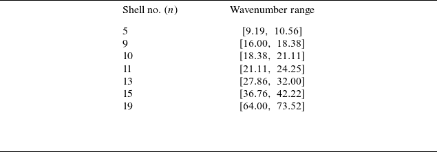

 Hn,mb,b
 n
 Hn,mb,j
 n
 m=n−1
 n−2
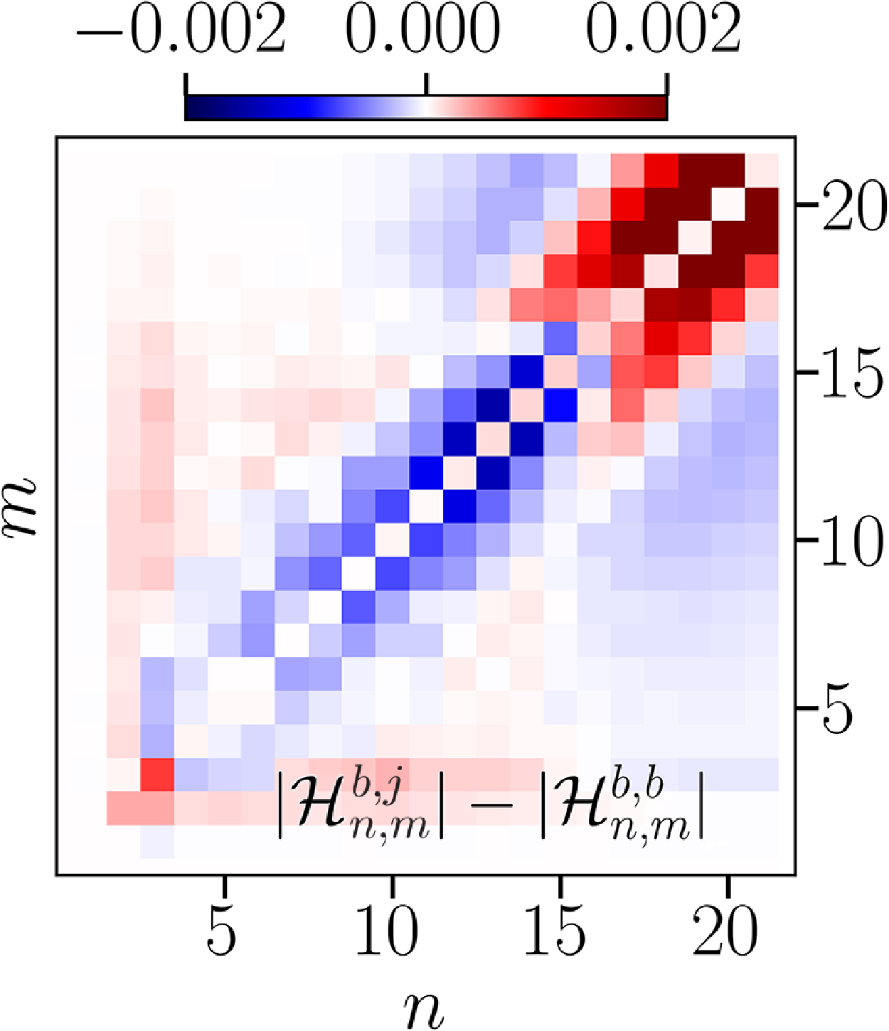
 |Hn,mb,j|−|Hn,mb,b|
 (m,n)

 Hn,m,ob,b
 (o,n)
 m
 Hn,m,ob,j
 (o,n)
 m
 |Hn,m,ob,j|−|Hn,m,ob,b|

 k

 k
 kH=50
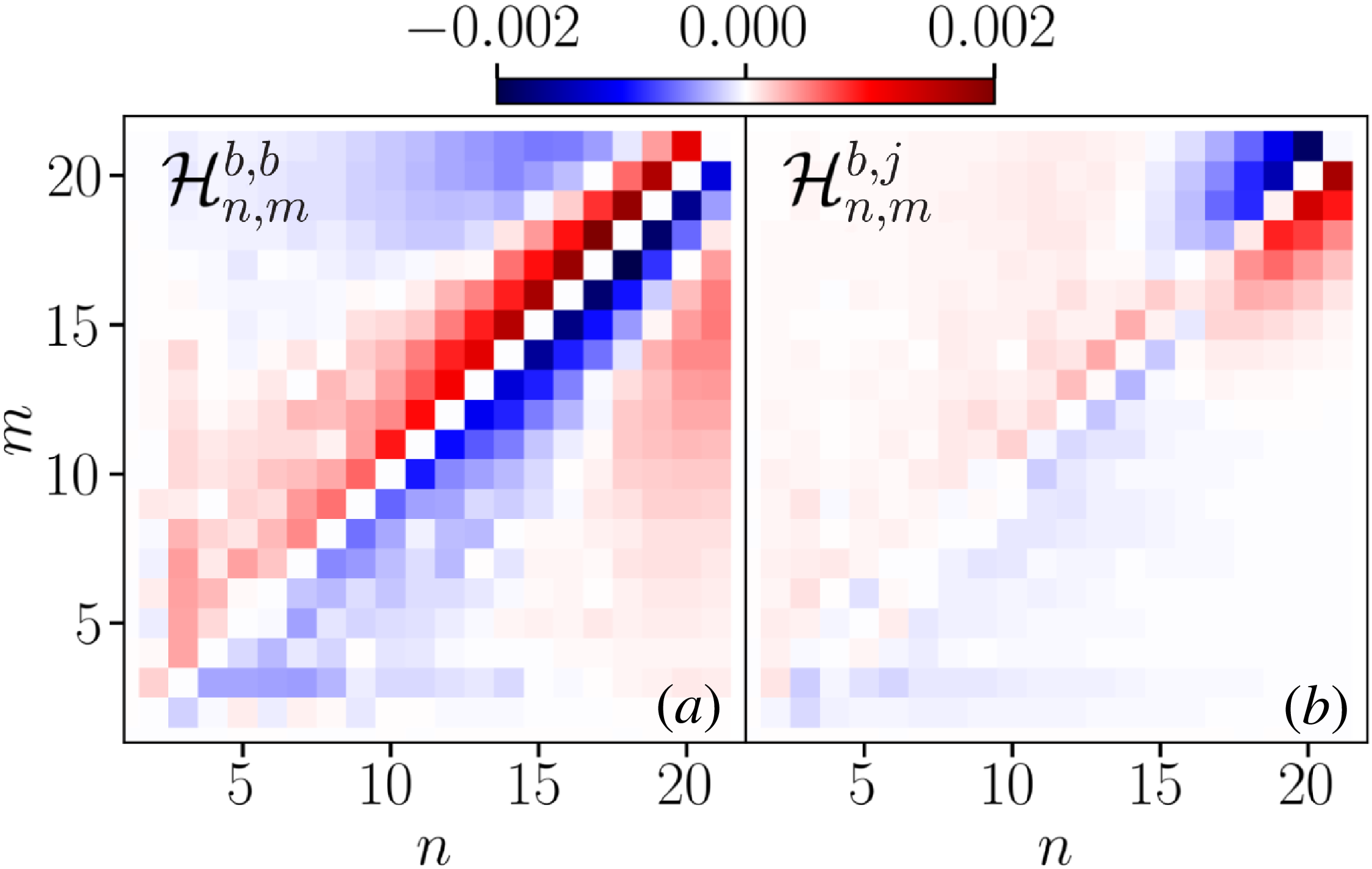
 BB
 JB
 kH=50
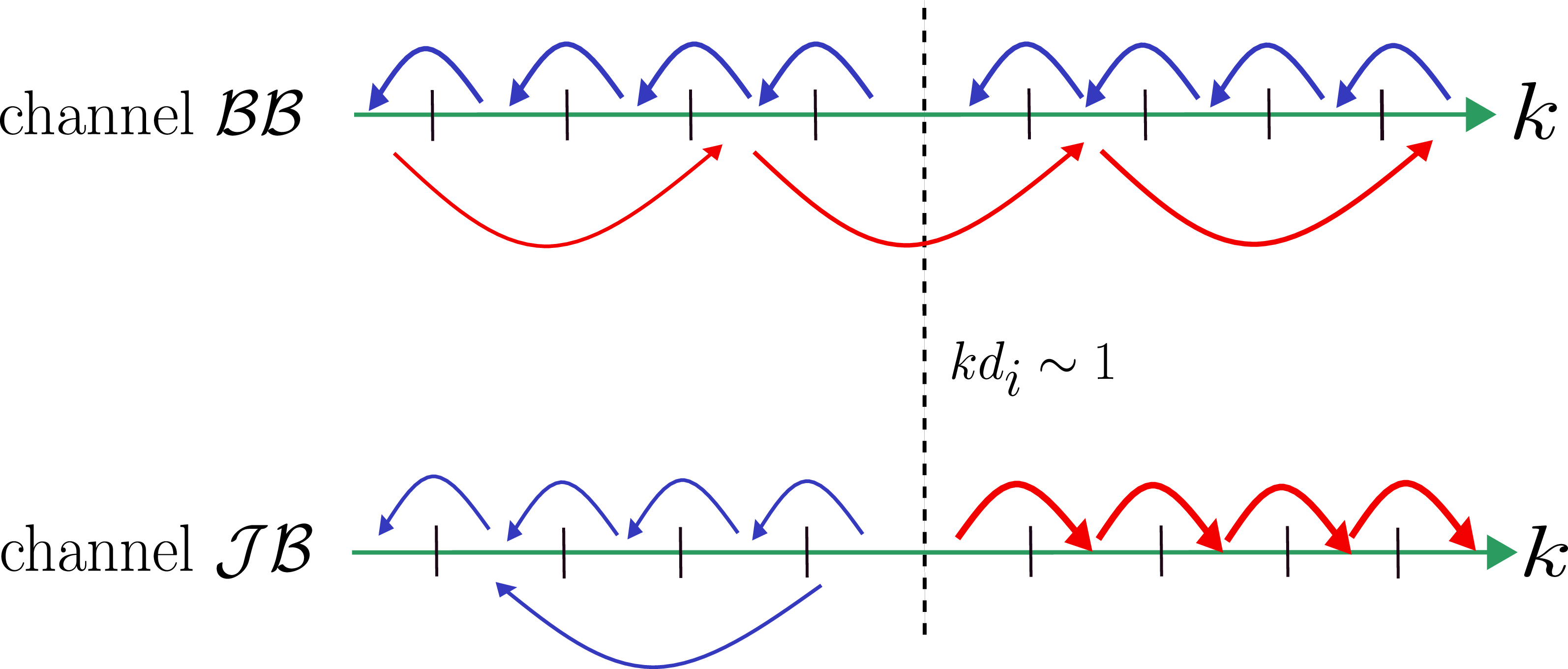

 Open access

