



1. Introduction
Preferential flow usually refers to a ‘winner-takes-all’ phenomenon of uneven fluid or solute transport in porous media, where the fluids prefer to travel through the low-resistance pathways rather than through other parts of the matrix. The frequent occurrence of this phenomenon has attracted much attention from biochemists, hydrologists, agriculturalists and geophysicists, for its close relevance to numerous practical issues, such as drug delivery in vascular networks (Kim, Park & Lee Reference Kim, Park and Lee2017; Jensen & Chernyavsky Reference Jensen and Chernyavsky2019), soil wetting (Homsy Reference Homsy1987; Valentine, Zhang & Robinson Reference Valentine, Zhang and Robinson2002; Šimůnek et al. Reference Šimůnek, Jarvis, Van Genuchten and Gärdenäs2003; Good, Noone & Bowen Reference Good, Noone and Bowen2015), enhanced oil recovery (EOR) (Payatakes Reference Payatakes1982; Gerritsen & Durlofsky Reference Gerritsen and Durlofsky2005; Thomas Reference Thomas2008; Zinchenko & Davis Reference Zinchenko and Davis2017; Singh et al. Reference Singh, Jung, Brinkmann and Seemann2019) and microfluidic logic control (Fuerstman, Garstecki & Whitesides Reference Fuerstman, Garstecki and Whitesides2007; Prakash & Gershenfeld Reference Prakash and Gershenfeld2007; Gasperino et al. Reference Gasperino, Baughman, Hsieh, Bell and Weigl2018). As opposed to uniform flow, preferential flow is one of the most unwelcome flow patterns during the above processes. For example, in reservoir engineering, when preferential water paths (fingers) form, oil recovery in the remaining parts of the reservoir is drastically reduced (Homsy Reference Homsy1987). This effect may lead to a considerable amount of the remaining oil trapped underground, and therefore controlling and suppressing preferential flow, which is the theme of this paper, is of crucial importance.
Extensive efforts have been made to understand the mechanism of this flow pattern from the large scale (Adler & Brenner Reference Adler and Brenner1988; Ritsema et al. Reference Ritsema, Dekker, Hendrickx and Hamminga1993; Khan et al. Reference Khan, Koneshloo, Knappett, Ahmed, Bostick, Mailloux, Mozumder, Zahid, Harvey and Van Geen2016) down to the core-to-pore scale (Chen & Wilkinson Reference Chen and Wilkinson1985; Stokes et al. Reference Stokes, Weitz, Gollub, Dougherty, Robbins, Chaikin and Lindsay1986; Cueto-Felgueroso & Juanes Reference Cueto-Felgueroso and Juanes2008; Li et al. Reference Li, Lowengrub, Fontana and Palffy-Muhoray2009; Segre & Holtzman Reference Segre and Holtzman2015; Holtzman Reference Holtzman2016; Singh et al. Reference Singh, Jung, Brinkmann and Seemann2019). These results suggest that either applying to a more homogeneous matrix or providing more favourable flow conditions (e.g. controlling the flow rate, viscosity ratio and wettability) may lead to more stable and compact displacements. Advanced techniques for enhanced oil recovery, like foam or continuous polymer flooding, have shown success in suppressing preferential flow (Li et al. Reference Li, Yan, Liu, Hirasaki and Miller2010; Wever, Picchioni & Broekhuis Reference Wever, Picchioni and Broekhuis2011; Talebian et al. Reference Talebian, Masoudi, Tan and Zitha2014; Wei & Romero-Zer Reference Wei and Romero-Zer2014; Al Ayesh et al. Reference Al Ayesh, Salazar, Farajzadeh, Vincent-Bonnieu and Rossen2016). Dispersed polymer systems (non-soluble polymer drops/particles in water), including preformed particle-gel (PPG) solution (Bai et al. Reference Bai, Li, Liu, Liu, Wang and You2007a) and soft microgel (SMG) (Wu et al. Reference Wu, Xiong, Xu, Zhang, Lu, Lu, Li, Cao, Zhang and Cui2015), were further proposed to provide a better conformance control rather than the traditional continuous polymer solutions.
Laboratory core experiments have demonstrated their EOR performance, and the excellent capability of dispersed polymers for EOR has been ascribed to the plugging and diverting effect (Bai et al. Reference Bai, Liu, Coste and Li2007b; Wang et al. Reference Wang, Liu, Wang and Hou2012; Abdulbaki et al. Reference Abdulbaki, Huh, Sepehrnoori, Delshad and Varavei2014; Han et al. Reference Han, Alshehri, Krinis and Lyngra2014; Wu et al. Reference Wu, Xiong, Xu, Zhang, Lu, Lu, Li, Cao, Zhang and Cui2015). Researchers figured out the importance of size matching between the particles and pore throats for plugging. Bai et al. (Reference Bai, Liu, Coste and Li2007b) and Wu & Bai (Reference Wu and Bai2008) found that a sharp increase in pressure took place when the PPG size is relative to the pore-throat size. Zaitoun et al. (Reference Zaitoun, Tabary, Rousseau, Pichery, Nouyoux, Mallo and Braun2007) reported a field application of microgels in a gas storage reservoir and showed the existence of an optimal gel size of ~2 μm for plugging of the high-permeability layer. Dai et al. (Reference Dai, Liu, Zou, You, Yang, Zhao, Zhao, Wu and Sun2017) defined a matching factor to investigate the matching relationship between the particle size and the pore-throat size, and they found that the optimized matching factor ranged from 0.21 to 0.29. If the plugging effect was the only mechanism for EOR, the application of this method had to be very picky and limited. Meanwhile, nanoparticles were reported to be effective for EOR (Suleimanov, Ismailov & Veliyev Reference Suleimanov, Ismailov and Veliyev2011; Sun et al. Reference Sun, Zhang, Chen and Gai2017; Olayiwola & Dejam Reference Olayiwola and Dejam2019), whose size was much smaller than the throat size. Therefore, the mechanisms of dispersed polymer microparticles for robust applications have not been fully explored yet.
Challenges are faced in both experimental and numerical tools, and their combination, for studying the mechanisms. For experiments, the characterization of the mechanical properties of microparticles and the visualization and quantification of micro-flow and phase interaction of multiple phases are very crucial but challenging. For numerical simulations, to the best of our knowledge, there are few comprehensive models for modelling multiphase systems including dispersed polymers. The difficulties include: (1) three phases at least should be considered, including oil, water and polymers; (2) incorporation of complex viscoelastic non-Newtonian behaviour for the polymer solution is a necessity (Wang et al. Reference Wang, Cheng, Yang, Wenchao, Qun and Chen2000; Abdulbaki et al. Reference Abdulbaki, Huh, Sepehrnoori, Delshad and Varavei2014; Saghafi et al. Reference Saghafi, Naderifar, Gerami and Emadi2016); and (3) such an intricate flow system should be modelled in the complex solid porous geometries of rocks. In our previous work (Xie, Lv & Wang Reference Xie, Lv and Wang2018b), we reduced the problem to a two-phase flow system by treating the polymer in water as a well-mixed continuous phase with a viscoplastic behaviour according to their bulk rheological properties (Wever et al. Reference Wever, Picchioni and Broekhuis2011; Cohen-Addad, Höhler & Pitois Reference Cohen-Addad, Höhler and Pitois2013; Jung et al. Reference Jung, Zhang, Chon and Choi2013). Comparisons between the shear-thinning and shear-thickening fluids were reported by a two-phase numerical model for viscoplastic fluids (Xie et al. Reference Xie, Zhang, Bertola and Wang2016), which showed that merely shear rheological properties did not enhance the diversion as expected. This research further indicated the importance of directly considering three-phase (water, oil and dispersed polymer) fluid flow in porous media for revealing the mechanisms of EOR by dispersed polymers.
In this paper, we first examine the EOR performance of polymers containing microparticles in the microchip experiments in § 2. Inspired by the experimental observation, we perform pore-scale numerical simulations for oil displacement processes by a dispersed polymer system in heterogeneous porous media in § 3. By combination of experimental and numerical analysis, we figure out new mechanisms of dispersed polymers for preferential flow control (diversion), which may lead to new EOR techniques.
2. Experimental observation
In order to examine the effectiveness of polymer flooding with microsphere particles for preferential flow control in heterogeneous rocks, we first perform experiments. A microfluidic platform has been established to observe and characterize the displacement process by multiphase systems in heterogeneous porous media, as shown in figure 1(a) (Lei et al. Reference Lei, Liu, Xie, Yang, Wu and Wang2020). The microfluidic chip is made of silicon, consisting of two layers, a higher- and a lower-permeability layer, as shown in figure 1(b). The dimensions of the chip are 8.64 mm × 5.76 mm, with a depth of 60 μm. The diameter of the larger grains in the upper layer is 420 μm, while that of the smaller grains in the lower layer is 210 μm. The pore-throat sizes are 220–100 μm and 110–50 μm for the upper and the lower layers, respectively. In the experiments, a decane solution (molecular weight = 142.28 g mol−1, viscosity = 0.00073 mPa s−1, density = 678 kg m−3) is used as the oil phase. The fluorescent dispersed polymer (containing 20 wt % dispersed microsphere particles) was made by inverse micro-emulsion polymerization techniques and it is diluted to 3 vol % by deionized water in experiments.
Diagram of the microfluidic platform. (a) Experimental system of the platform. (b) Heterogeneous porous structure with two layers of microfluidic chip (black represents solid grains and yellow denotes flow region). (c) Microscope picture of the dispersed microsphere polymer.

The plugging mechanism of polymer particles has been proved and well understood when the pore/throat size is comparable to the particle size. In this study, we choose microparticles whose mean diameter is much smaller than the pore-throat size of porous media. The mean particle diameter of the microsphere particles in our experiments is 7.64 μm, as measured by Malvern Mastersizer (MS 3000). The microsphere particles are a network of aggregated colloidal particles with soft solid-like mechanical properties (Lei et al. Reference Lei, Xie, Wu, Wu and Wang2019), as shown in figure 1(c). The contact angle between the aqueous fluids and decane is 93.3°, as measured by the Drop Shape Analysis (DSA25, KRUSS) system. A constant flow rate is set at 1 μL min−1 by a syringe pump to inject all the displacing fluids.
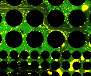
The process of dispersed polymer flooding is compared with that of deionized water flooding in figure 2(a,b) (see also the supplementary movies 1 and 2, available at https://doi.org/10.1017/jfm.2020.763). During deionized water flooding, the preferential flow path quickly forms in the higher-permeability layer, the upper part of the chip, leaving most oil residual in the lower part. Even though the mean diameter of the microsphere polymer particles is much smaller than the pore-throat size of both layers, it is surprisingly found that the dispersed polymer flooding process shows an evident diversion effect, as the displacing fronts in the upper part and lower part move forward alternately, and the lower front can even be ahead of the upper front (0.33 PV, PV = pore volume). Figure 2(c) presents enlarged views of two adjacent snapshots during dispersed polymer flooding. Yellow denotes the oil phase, dark is the displacing phase, and the dispersed microspheres are dyed as green. As noted by the circled area and the red arrow, the dispersed microspheres are diverted from the upper layer to the lower layer at this moment when the upper layer stays blocked. These observations confirm the advantages of the dispersed polymer microparticles by providing a diversion effect for preferential flow control. Since the microsphere particle size is much smaller than the pore-throat size, the plugging mechanism proposed by previous researchers may not explain the diversion behaviour fully. The experiments examine the effect qualitatively, but hardly reveal the phase interactions and diversion effects quantitatively. Therefore, in order to discover the remaining mechanisms, we further perform pore-scale numerical simulations.
Displacing processes of (a) deionized water flooding and (b) dispersed microsphere polymer flooding in the microfluidic chip. (c) Enlarged view of two adjacent snapshots during dispersed polymer flooding illustrating the diversion of the dispersed microsphere. Yellow denotes the oil phase, dark parts are the displacing phase, and the dispersed microspheres are dyed as green.

3. Numerical simulation and mechanism analysis
A powerful numerical tool for multiphase flow in porous media is necessary to study this problem comprehensively. The lattice Boltzmann (LB) methods for multiphase flow have been validated against experiments or empirical models and have exhibited excellent performance on predicting multiphase flow in simple porous media (Jiang & Tsuji Reference Jiang and Tsuji2017; Zhao et al. Reference Zhao, MacMinn, Primkulov, Chen, Valocchi, Zhao, Kang, Bruning, McClure and Miller2019). Recently, we have also developed an LB framework for three-phase complex fluid flows with viscoelastic or viscoplastic properties (Xie, Lei & Wang Reference Xie, Lei and Wang2018a), which has proved excellent for mass conservation, numerical accuracy and stability for complex geometries. This model is based on an improved Rothman–Keller type LB method (Leclaire, Reggio & Trépanier Reference Leclaire, Reggio and Trépanier2013; Leclaire & Pellerin Reference Leclaire and Pellerin2014) for immiscible multiphase flow with accurate mass conservation for each phase, which is essential for fluid displacement in porous media. It applies N (number of fluids) sets of LB equations to describe the movement of each fluid denoted by k, with each equation being a similar form as
 \begin{equation}f_i^k(\boldsymbol{x} + {\boldsymbol{c}_i}\mathrm{\Delta }t,t + \mathrm{\Delta }t) - f_i^k(\boldsymbol{x},t) = \varOmega _i^k(\,f_i^k(\boldsymbol{x},t)) + \varGamma_i \left( {\frac{{{\rho_k}}}{\rho }\boldsymbol{F}(\boldsymbol{x},t)} \right),\end{equation}
where  $f_i^k$ is the distribution function of fluid k in the ith velocity direction, x the lattice position, t the time, Δt the time step, and
 ${\boldsymbol{c}_i}$ the lattice speed. In addition,
 ${\rho _k}$, ρ and u are the macroscopic phase density, total density and flow velocity, respectively;
 $\varOmega _i^k$ is the collision operator to govern the momentum evolution and interfacial dynamics, and to ensure mass conservation for each phase; and
 ${\varGamma _i}$ is the forcing term to account for the body force F including gravity ρg (g is the gravitational acceleration) (Guo, Zheng & Shi Reference Guo, Zheng and Shi2011) and the viscoelastic force
 ${\boldsymbol{F}_{el}}$.
The Maxwell constitutive relation is correctly introduced into the momentum equation to account for the viscoelastic behaviour of polymers (Saghafi et al. Reference Saghafi, Naderifar, Gerami and Emadi2016). The viscoelastic body force  ${\boldsymbol{F}_{el}}$ of a Maxwell fluid is derived as
 \begin{equation}{\boldsymbol{F}_{el}}(\boldsymbol{x},t) = \boldsymbol{\nabla} \boldsymbol{\cdot}\boldsymbol{\sigma }=\frac{{{\eta _p}}}{{{\tau _{el}}}}\int_{ - \infty }^{\boldsymbol{t}} \exp \left( { - \frac{{t - t^{\prime}}}{{{\tau_{el}}}}} \right) {\nabla ^2}\boldsymbol{u}(\boldsymbol{x},t^{\prime})\,\textrm{d}t^{\prime},\end{equation}
where  $\boldsymbol{\sigma }$ is the Cauchy stress tensor,
 ${\eta _p}$ the polymer intrinsic dynamic viscosity, E the elastic modulus and
 ${\tau _{el}} = {\eta _p}/E$ the viscoelastic relaxation time.
Combined with the proper statistical relations for the distribution functions (Xie et al. Reference Xie, Lei and Wang2018a), the above LB equations can recover the following governing equations at continuum scale for this problem:
 \begin{gather}\boldsymbol{\nabla} \boldsymbol{\cdot}(\rho \boldsymbol{u}) = 0,\end{gather}
 \begin{gather}{\partial _t}\rho \boldsymbol{u} + (\boldsymbol{u}\boldsymbol{\cdot}\boldsymbol{\nabla})\rho \boldsymbol{u} ={-} \boldsymbol{\nabla} \boldsymbol{\cdot}p\boldsymbol{\boldsymbol{\mathsf{I}}} + \boldsymbol{\nabla} \boldsymbol{\cdot}\boldsymbol{\sigma } + \rho \boldsymbol{g} + {\boldsymbol{F}_\gamma },\end{gather}
where p is the pressure,  ${\boldsymbol{F}_\gamma }$ is in charge of the interfacial tension
 $\gamma $, and
 ${\boldsymbol{\mathsf{I}}}$ the identity tensor,
 \begin{equation}\boldsymbol{\nabla} \boldsymbol{\cdot}\boldsymbol{\sigma } = \eta {\nabla ^2}\boldsymbol{u}\quad (\hbox{for Newtonian fluids: water and oil in this paper})\end{equation}
or
 \begin{equation}\dot{\varepsilon } = \frac{\boldsymbol{\sigma }}{{{\eta _p}}} + \frac{1}{E}\frac{{\textrm{d}\boldsymbol{\sigma }}}{{\textrm{d}t}}\quad (\hbox{for viscoelastic polymer}),\end{equation}
where  $\eta $ is the dynamic viscosity and
 $\dot{\varepsilon }$ the strain rate.
The numerical algorithm to solve the above equations is given in appendix A. The verifications of the numerical model for capturing correct three-phase momentum evolution, wettability and viscoelastic features are presented in appendix B. To simulate the dispersed polymer flooding, the schematic of the computational domain and the initial fluid configurations are illustrated in figure 3. According to the convergence study shown in appendix C, we apply a 901 × 452 lattice to cover the whole domain. On the left side of the main porous region, a ‘dispersed polymer generation device’ is included using a 214 × 452 lattice inspired by the microfluidic techniques (Gunther & Jensen Reference Gunther and Jensen2006). We construct three inlet pipes with the same width of 22 lattices in the left buffer, where the polymers, injected from the left with the area flow rate Qp, are cut into dispersed drops by the water on two sides with a flow rate Qw 1. We also add another two inlets with the width of 11 lattices for additional water to come in with a flow rate Qw 2, which is used to adjust the polymer concentration while keeping the ratio of Qp/Qw 1 to successfully generate the dispersed polymers.
Schematic of the domain and the initial fluid configurations for dispersed polymer flooding simulation. Black represents the solid grain or boundaries, red represents the oil, blue represents the water and green represents the polymer. The permeability ratio between the upper and lower parts of the main porous medium is 3.11 according to our single-phase calculations. The left buffer is desired for water and dispersed polymer injection.

Three groups of displacements are considered, continuous water flooding, continuous polymer flooding and dispersed polymer flooding. The two-phase continuous water flooding and the continuous polymer flooding cases are considered by changing the left pipe to water injection and the two cutting pipes to polymer injection, respectively. In our simulations, a time step  $\Delta t = 2.13 \times {10^{ - 6}}\ \textrm{s}$ and a lattice spacing
 $\Delta x = 12.8\;\mu \mathrm{m}$ are used to satisfy the criteria set in Xie et al. (Reference Xie, Lei and Wang2018a). Gravity effects are negligible in the x–y plane. The inlet boundary parameters are the given flow rates (Guo & Zheng Reference Guo and Zheng2002) for five inlets, and the outlet boundary condition is a convective outflow boundary (Lou, Guo & Shi Reference Lou, Guo and Shi2013). Unless otherwise specified, the left injection rate is set at
 ${Q_p} = 3.5 \times {10^{ - 6}}\;{\textrm{m}^2}\ {\textrm{s}^{ - 1}}$ with a cutting flow rate set at
 ${Q_{w1}} = 8.5 \times {10^{ - 6}}\ {\textrm{m}^2}\ {\textrm{s}^{ - 1}}$ from the upper and lower sides, and the adjusting flow rate is set at Qw 2 = 0. These conditions result in a flow rate ratio of 7 : 17 that ensures a stable generation of dispersed polymer drops. Other parameters in the simulations are
 ${\rho _w} = 1000\;\textrm{kg}\ {\textrm{m}^{ - 3}}$,
 ${\rho _o} = 678\ \textrm{kg}\ {\textrm{m}^{ - 3}}$ and
 ${\rho _p} = 920\ \textrm{kg}\ {\textrm{m}^{ - 3}}$; the dynamic viscosities are
 ${\eta _w} = 0.00091\;\textrm{Pa}\ \textrm{s}$,
 ${\eta _o} = 0.02\ \textrm{Pa}\ \textrm{s}$ and
 ${\eta _p} = 0.025\;\textrm{Pa}\ \textrm{s}$; the interface tensions are
 ${\gamma _{wo}} = 0.006\;\textrm{N}\ {\textrm{m}^{ - 1}}$,
 ${\gamma _{pw}} = 0.005\;\textrm{N}\ {\textrm{m}^{ - 1}}$ and
 ${\gamma _{op}} = 0.005\;\textrm{N}\; {\textrm{m}^{ - 1}}$; the contact angles on solid grains are set as
 ${\theta _{wo}} = 90^\circ $,
 ${\theta _{pw}} = 155^\circ $ and
 ${\theta _{op}} = 25^\circ $. Note that the neutral–wet condition is selected at the water–oil–grain interfaces here just for mechanism study to exclude other factors, such as the capillary effects, which could also affect the flow preference (Morrow & Mason Reference Morrow and Mason2001), to avoid interfering with the main theme of this study. Therefore, for the two-phase continuous polymer displacements, the oil–polymer contact angle is set as
 ${\theta _{op}} = {\theta _{wo}} = 90^\circ $ in order to be comparable with the two-phase water flooding case.
The displacing processes are shown in figure 4 (see also the supplementary movies 3–5) and the evolutions of pressure distribution are shown in figure 5 (see also the supplementary movies 6–8), respectively. The preferential flow paths form in the higher-permeability layer of the porous structure immediately for continuous water flooding, which suppresses the driving pressure in the lower-permeability layer. The continuous polymer solution has a very high viscosity, e.g. the momentum transfer capability, to even the driving pressure of both layers. As a result, the polymer flooding has a much higher oil recovery than the water flooding, which is also indicated quantitatively in figure 6(a). This can also be explained by the well-established knowledge of mobility/viscosity ratio control for more stable displacement. However, although the effective viscosity of the dispersed polymer system with a smaller amount of polymer is smaller than the continuous polymer solution, its performance is surprisingly even better than the continuous polymer flooding. This could be explained by the automatic diversion of the dispersed polymers, which induces a larger pressure fluctuation. As illustrated in figure 6(b) and qualitatively in figure 5, the dispersed polymer flooding has the most remarkable fluctuation of pressure than the other two flooding processes.
Displacing processes of (a) continuous water flooding, (b) continuous polymer flooding and (c) dispersed polymer flooding. The cumulative injection volume of fluids normalized by the pore volume (PV) of the main porous region is used to denote the displacing time.

Evolution the corresponding pressure distribution during (a) continuous water flooding, (b) continuous polymer flooding and (c) dispersed polymer flooding.

Evolutions of (a) the total oil saturation in the main porous region and (b) the pressure drop through the porous medium. Mean pressures at the left and right sides of the porous medium are counted as the inlet and outlet pressure, respectively.

Something inspiring can be found from comparisons between the dispersed polymer flooding and the water flooding. Before breakthrough at the higher-permeability layer, the differences in the pressure distributions are small, because the driving pressure can transfer farther in the region with a lower resistance, which leads to the formation of preferential flow paths for each case, as shown in figure 5(a,c) at 0.11 PV. Later on, the pressure distribution reverses for the dispersed polymer flooding as more and more polymers with higher viscosity are squeezed into the higher-permeability layer, resulting in increase of resistance there, while the pressure contour keeps the same shape for the water flooding, as shown in figure 5(a,c) during 0.45–0.75 PV. Sequentially, the dispersed polymer solution switches pathways between the higher- and lower-permeability layers in the heterogeneous porous structure based on the resistance and consequent driving pressure changes. The result is an induced pressure fluctuation during the displacement process and the benefit is the significantly enhanced sweeping area. Such fluctuations never happen for the water flooding and the pressure distributions. These processes are shown in figure 5(a,c) during 0.75–4.20 PV. The pressure fluctuation plays a significant role in EOR, as it helps to activate the original hard-to-displace oil and to reduce the residual oil, as shown in figure 4(c) compared with figure 4(a,b) at 4.20 PV. As to the two-phase continuous polymer flooding, though the preferential flow is suppressed to the largest extent at the initial stage, leading to an almost flat pressure contour, there is no fluctuation induced, as shown in figure 5(b), because its principle for preferential flow control lies only in the higher viscosity of the displacing fluids.
The qualitative analysis above illustrates what happens in detail for continuous water flooding, continuous polymer flooding and dispersed polymer flooding in the heterogeneous porous structure. Since they are simulated numerically, especially for the polymer–water–oil three-phase flow system for the first time, a quantitative comparison can be made in this work. As is well known, the benefits and the costs are a contradictory pair. The benefit of using polymer for EOR is very clear, e.g. increase of oil recovery rate, which could be characterized by the residual oil saturation. The cost comes from at least two points: one from increased driving force for displacing fluids, and the other from the expense of the polymer materials. An optimal EOR scheme needs a balance between the benefits and the costs. Our numerical tool makes it possible to compare the schemes quantitatively.
The local evolutions of pressure and oil saturation have been exactly captured by our simulations, which are shown in figure 6. Figure 6(a) indicates that using polymers, either continuous or dispersed ones, is effective for EOR. Compared with the water flooding, both continuous and dispersed polymer flooding reduce the final oil saturation by over 30 %. The oil recovery from continuous polymer flooding is quicker than that from dispersed flooding, yet the final oil recovery rates are close and the dispersed one has less residual oil left behind. The evolution curves of pressure drop are shown in figure 6(b), which indicates that continuous polymer flooding needs much higher driving pressure than the dispersed one. After statistically averaging the fluctuating pressure drops after 1 PV of the dispersed polymer flooding, we find this value is only 38 % of the continuous polymer flooding. This means that the dispersed polymer flooding can save much pumping power for displacing fluids and is more suitable for low-permeability reservoirs compared with continuous polymer flooding. In addition, dispersed polymer flooding needs much less polymer material, which is also a big cost for EOR. Therefore, the dispersed polymer flooding method can improve the oil recovery in a more intelligent and efficient way, with a better performance for even tougher reservoir conditions compared with continuous polymer flooding.
Furthermore, we characterize the diversion effect, which suppresses the preferential flow via the oil saturation difference between the lower and upper parts of the heterogeneous porous medium in figure 7(a). With a smaller difference indicating a stronger diversion effect, the poorest profile is not surprisingly found in the water flooding. Here we focus on comparisons between the two polymer flooding cases. Similar to the fluctuating pressure profile of dispersed polymer flooding in figure 6(b), the oil saturation difference curve shows fluctuations as well in figure 7(a). Moreover, the upward or downward shifts in the oil saturation difference curve correspond to different stages in accordance with different displacing processes, each of which is characterized by a corresponding inset in figure 7(a).
Evolutions of the oil saturation differences between the lower and upper parts of (a) the regular packed porous medium and (b) the complex porous medium. Smaller values indicate stronger suppression of the preferential flow.

In the first stage, all three curves quickly go up during the initial formation of preferential flow paths, and the continuous polymer flooding case offers the best control of it because of its higher viscosity. The sharp rising stages end around the breakthrough of the upper layer, and then these curves enter the second stage. The curves of the two polymer flooding cases turn down after the upper layers are almost saturated, yet there is enough room for oil in the lower layers to be displaced slowly. As seen in the second stage, the dispersed polymer system shows even better diversion capability. During this period (0.45–0.75 PV), all higher viscous polymers are automatically squeezed into the high-permeability upper layer while more water is diverted into the lower layer. Thus the dispersed polymer creates the largest difference in viscous property between the two layers and redistributes the flow resistances, leading to better diversion. As the cumulative increase of the resistance in the upper layer reaches some critical value, the dispersed polymers will ‘feel’ the change of resistance and pressure reverse, and part of them will begin to penetrate into the lower layer (0.75 PV). Afterwards, the curve turns distinctly upwards for the dispersed polymer case as the third stage, since the polymers keep entering into both layers (0.75–1.26 PV), which slightly weakens the diversion effect. Again, it turns downwards in the fourth stage, as all the polymers turn into the upper layer, enhancing the diversion due to their smart adaptions to the pressure and resistance (e.g. 2.41 PV). On the other hand, for the continuous polymer flooding case, the turning-down trend in the second stage continues with a decreasing slope as the lower layer also approaches saturated. Although the diversion effect of the dispersed polymer system is not always better than that of the continuous polymer system, it is this kind of intelligent self-adaption that provides the helpful pressure fluctuations for EOR mentioned above.
In addition to the regular packed porous geometry, we also consider a porous medium with a complex geometry close to that of real rocks, which was used in our previous study (Xie et al. Reference Xie, Lv and Wang2018b). The permeability ratio of this heterogeneous complex structure is 4.68, indicating that the difference between the two layers is larger than that of the regular geometry. Evolutions of the oil saturation differences for the complex geometry are shown in figure 7(b). The oil saturation difference curve for the dispersed polymer flooding also shows clear upward and downward stages, and the insets present similar self-adaptive diversion processes. Compared with the regular structure, the diversion effect in the complex geometry is even more prominent, as the red curve remains lower for a wider range of pore volume. These results illustrate the effectiveness of preferential flow control by using dispersed polymers in real porous media.
Moreover, the effect of polymer concentration on the capability for preferential flow control is investigated. This capability is quantified by the difference in pore volume injected for the occurrence of breakthrough at the lower and upper parts of the regularly packed porous medium. For all cases, we still keep the total flow rate at 1.2 × 10⁻⁵ m2 s−1 and the ratio between Qp and Qw 1 at 7 : 17. By adjusting the flow rate Qw 2 from 0 to 9.94 × 10⁻⁶ m2 s−1, we obtain different polymer concentrations at 29 %, 25 %, 20 %, 15 %, 10 % and 5 %. The phase distributions at the breakthrough moments for different polymer concentrations are presented in figure 8. The differences in pore volume injected are then plotted against polymer concentration in figure 9. These figures show that the capability for preferential flow control enhances with increasing polymer concentration, because more polymers are able to provide a bigger difference in the viscous property between the two layers. However, the enhancement is not as great as it is at low concentrations when the polymer concentration reaches about 20 %.
The phase distributions at the breakthrough moments in (a) the upper half and (b) the lower half for different polymer concentrations.

The effect of polymer concentration on the capability for preferential flow control by dispersed polymer flooding.

4. Conclusions
In conclusion, we investigate the mechanisms of preferential flow control by dispersed polymers via micro-model experiments and pore-scale simulations. The experimental observation confirms the diversion effect of dispersed microsphere particles with much smaller sizes than the pore-throat size. Through pore-scale modelling, we demonstrate that the dispersed polymer system provides preferential flow control and improves the oil recovery in a smarter and more efficient way. It saves the energy cost by 60 %, in particular, and shows even better performance than continuous polymer flooding in removing the remaining oil. In addition to the mechanisms of plugging and mobility/viscosity ratio control, new mechanisms are discovered for the dispersed system. The movements of dispersed polymers intelligently adapt to the changes of pressure and flow resistance, thus automatically controlling the preferential flow and fluctuating the driving pressure, which further benefit oil recovery. We further find that the capability for preferential flow control drastically enhances with increasing polymer concentration at low concentrations (<20 %). However, the enhancement is not that significant when the polymer concentration is larger than 20 %. The outcomes and novel understandings from this study can direct more effective polymer injection for enhanced oil recovery and may also lead to new designs for microfluidic systems.
Acknowledgements
M.W. gratefully acknowledges support from the National Key Research and Development Programme of China (No. 2019YFA0708704), the NSF grant of China (No. U1837602) and the Tsinghua University Initiative Scientific Research Programme. M.T.B. acknowledges the Chemical EOR Industrial Affiliates Project in the Center for Subsurface Energy and the Environment at The University of Texas at Austin. Our simulations are run on the ‘Explorer 100’ cluster of Tsinghua National Laboratory for Information Science and Technology.
Declaration of interests
The authors declare no conflict of interest.
Supplementary movies
Supplementary movies are available at https://doi.org/10.1017/jfm.2020.763.
Appendix A. Numerical procedure
The numerical algorithm for a single time step is given as follows:
(1) Given the values of
 $f_i^k(\boldsymbol{x},t)$, ${\boldsymbol{F}_{el}}(\boldsymbol{x},t)$ and $\boldsymbol{u}(\boldsymbol{x},t)$ from the last time step.
(2) Perform the streaming process of
$f_i^k(\boldsymbol{x},t)$.(3) Use the inlet and outlet boundary conditions to get the unknown
$f_i^k(\boldsymbol{x},t + \Delta t)$ on the open boundaries.(4) Use bounce-back rules to get the unknown
$f_i^k(\boldsymbol{x},t + \Delta t)$ on the solid boundary.(5) Compute the derivatives of
$\boldsymbol{u}(\boldsymbol{x},t)$ to get $\boldsymbol{\nabla}\boldsymbol{u}$.(6) Update the macroscopic variables
$\rho (\boldsymbol{x},t + \Delta t)$, ${\rho _k}(\boldsymbol{x},t + \Delta t)$, $\boldsymbol{u}(\boldsymbol{x},t + \Delta t)$ and ${\boldsymbol{F}_{el}}(\boldsymbol{x},t + \Delta t)$.(7) Compute the derivatives of colour gradients.
(8) Obtain the equilibrium distribution function
$f_i^{k,eq}(\boldsymbol{x},t + \Delta t)$.(9) Perform the collision process to evolve the LB equation (3.1) and to obtain
$f_i^k(\boldsymbol{x},t + \Delta t)$.(10) Increase the time step and go back to step 1 to start another cycle until the desired time step has been reached.


Appendix B. Verifications of numerical methods
Here we present three benchmark cases to verify the model from different aspects, including momentum transfer, wettability and viscoelasticity, which are three key factors for a close simulation for the problem of oil displacement by dispersed polymers in porous media.
B.1. Momentum transfer at the interface
In this case, a four-layer Couette flow driven by the upper plate with a wall velocity  ${u_w} = 0.01\;\textrm{m}\ {\textrm{s}^{ - 1}}$ is considered. The sketch of this problem is shown in figure 10(a). The fluids are placed in parallel between two infinite plates, with a red (r) fluid on two sides and a blue (b) and a green (g) fluid in the middle. The width of each fluid layer is
 $h = 3\;\textrm{mm}$. The densities and kinematic viscosities of these fluids are
 ${\rho _r} = 1000\ \textrm{kg}\ {\textrm{m}^{ - 3}}$,
 ${\nu _r} = 1 \times {10^{ - 6}}\ {\textrm{m}^2}\ {\textrm{s}^{ - 1}}$,
 ${\rho _g} = 100\ \textrm{kg}\ {\textrm{m}^{ - 3}}$,
 ${\nu _g} = 5 \times {10^{ - 6}}\ {\textrm{m}^2}\ {\textrm{s}^{ - 1}}$, and
 ${\rho _b} = 350\;\textrm{kg}\ {\textrm{m}^{ - 3}}$,
 ${\nu _b} = 9 \times {10^{ - 6}}\ {\textrm{m}^2}\ {\textrm{s}^{ - 1}}$, respectively. The fluid domain is covered by a
 $10 \times 122$ lattice in our simulation. We apply periodic boundary conditions on the left and right, the bounce-back rule on the lower stationary plate, and a moving boundary condition (Ladd Reference Ladd1994; Ladd & Verberg Reference Ladd and Verberg2001) on the upper moving plate. The interface tensions between the fluids are all set as
 $\gamma = 0.01\;\textrm{N}\ {\textrm{m}^{ - 1}}$. The cross-sectional momentum profile in the steady state is obtained in figure 10(b), which matches well with the theoretical solutions calculated by Leclaire et al. (Reference Leclaire, Reggio and Trépanier2013).
Validation of momentum transfer at interfaces by comparison of simulation results with theoretical solutions for a four-layer Couette flow. (a) The sketch of the physical problem. (b) The cross-sectional momentum profiles in the steady state.

B.2. Three-phase wettability
In this case, we examine the validity of this model to capture three-phase fluid–fluid and fluid–solid interactions. As shown in figure 11(a), the three-phase system in contact with a solid plate is considered. Two symmetrical quarter-circular droplets (green and blue fluids with initial radius  ${R_0} = 2.5\;\textrm{mm}$) are initially placed closely in contact with each other on the bottom plate, surrounded by another bulk fluid (red). Densities and kinematic viscosities of the fluids are
 ${\rho _r} = 1000\;\textrm{kg}\ {\textrm{m}^{ - 3}}$,
 ${\nu _r} = 1 \times {10^{ - 4}}\ {\textrm{m}^2}\ {\textrm{s}^{ - 1}}$,
 ${\rho _g} = 200\ \textrm{kg}\ {\textrm{m}^{ - 3}}$,
 ${\nu _g} = 1 \times {10^{ - 4}}\ {\textrm{m}^2}\ {\textrm{s}^{ - 1}}$, and
 ${\rho _b} = 800\, \textrm{kg}\ {\textrm{m}^{ - 3}}$,
 ${\nu _b} = 1 \times {10^{ - 4}}\;{\textrm{m}^2}\ {\textrm{s}^{ - 1}}$, respectively. Owing to the interactions between fluids and solid, the relationship between interface tensions and contact angles follows (Semprebon, Krüger & Kusumaatmaja Reference Semprebon, Krüger and Kusumaatmaja2016):
 ${\gamma _{rg}}\cos {\theta _{rg}} + {\gamma _{gb}}\cos {\theta _{gb}} + {\gamma _{br}}\cos {\theta _{br}} = 0$.
Validation of three-phase contacts. (a) Sketch of three-phase contacts. (b,c) Equilibrium three-phase distributions obtained by simulations for the prescribed contact angles of (b)  ${\theta _{gr}} = 45^\circ $,
 ${\theta _{gb}} = 45^\circ $ and
 ${\theta _{br}} = 90^\circ $ and (c)
 ${\theta _{gr}} = 90^\circ $,
 ${\theta _{gb}} = 60^\circ $ and
 ${\theta _{br}} = 145^\circ $.

Two groups of simulations are performed using  ${\theta _{gr}} = 45^\circ $,
 ${\theta _{gb}} = 45^\circ $ and
 ${\theta _{br}} = 90^\circ $ for group (b) and
 ${\theta _{gr}} = 90^\circ $,
 ${\theta _{gb}} = 60^\circ $ and
 ${\theta _{br}} = 145^\circ $ for group (c). The interface tensions between phases are all set as
 $\gamma = 0.01\;\textrm{N}\ {\textrm{m}^{ - 1}}$. The simulation domain covers a
 $100 \times 42$ lattice. The wetting boundary conditions with the prescribed values are imposed on the lower plate. The phase distributions in the equilibrium states are shown in figure 11(b,c), which demonstrate that the evolved contact angles match well the prescribed values for both groups.
B.3. Multiphase viscoelasticity
The captured viscoelasticity is validated here by a Newtonian bubble rising in a viscoelastic fluid. The bubble with an initial radius of R is released in a closed tank filled with the bulk viscoelastic fluid. The bubble will rise driven by the buoyancy force. If the capillary number (Ca) and the Deborah number (De) are relatively large, there will appear a sharp tip at the tail of the bubble, and a ‘negative wake’ region because of the viscoelastic memory effect (Liu, Liao & Joseph Reference Liu, Liao and Joseph1995; Pillapakkam et al. Reference Pillapakkam, Singh, Blackmore and Aubry2007; Fraggedakis et al. Reference Fraggedakis, Pavlidis, Dimakopoulos and Tsamopoulos2016).
We perform numerical simulations for the bubble rising dynamics in a viscoelastic fluid or in a Newtonian fluid. We choose parameters that lead to a capillary number of  $Ca = 21.2$ and a Deborah number of
 $De = 4.04$. The bubble rising evolutions are shown in figure 12(a,b). The ‘cusp shape’ of the bubble is well captured for the viscoelastic case, in contrast to the Newtonian one. The streamlines during bubble rising are shown in figure 12(c,d). The ‘negative wake’ region behind the bubble and two vortex rings are captured in the viscoelastic case, while they are never found in the Newtonian case. These results indicate that our model well captures the viscoelastic features.
Bubble shape evolution and streamline snapshots during bubble rising processes. (a) Bubble shape evolution in a Newtonian fluid. (b) Bubble shape evolution in a viscoelastic fluid. (c) Snapshot of streamline during bubble rising in a Newtonian fluid. (d) Snapshot of streamline during bubble rising in a viscoelastic fluid. The tank size is  $L \times H = 20\; \;\textrm{mm} \times 40\;\textrm{mm}$ divided into a
 $201 \times 401$ lattice grid. Closed wall boundary conditions with completely bulk fluid-wetting conditions are applied on all walls. For the Newtonian bubble:
 ${\rho _b} = 100\;\textrm{kg}\ {\textrm{m}^{ - 3}}$ and
 ${\eta _b} = 0.015\;\textrm{Pa}\ \textrm{s}$. The initial radius of the bubble is
 $R = 3\;\textrm{mm}$. Other parameters are
 $g = 9.8\;\textrm{m}\ {\textrm{s}^{ - 2}}$ and
 $\gamma = 0.01\;\textrm{N}\ {\textrm{m}^{ - 1}}$. For the bulk fluids:
 ${\eta _p} = 0.875\;\textrm{Pa}\ \textrm{s}$. The viscoelastic relaxation time of the viscoelastic fluid is
 ${\tau _{el}} = 0.1\;\textrm{s}$.

Appendix C. Convergence study
We select three grids to perform the convergence tests on the default dispersed polymer flooding case. All the physical parameters are kept the same, except the domain size, the lattice space and the time step listed in table 1. We use different time steps for different grids to ensure the same relaxation time in the LB equation.
Parameters for convergence tests.

Figure 13 presents the comparisons of (a) the oil saturation evolution curves and (b) phase distributions at 0.24 PV obtained by simulations using different grids. As is seen, the oil saturation curves almost collapse for the medium grid  $(901 \times 452)$ and the large grid
 $(1201 \times 602)$ cases, while the small grid (601 × 302) result deviates from them. For the phase distributions at 0.24 PV, the medium grid result is similar to the large grid result, where all of the polymers go to the higher-permeability layer and water is just about to penetrate into the lower-permeability layer; however, the small grid result is much different.
Convergence tests for the dispersed polymer flooding case. (a) Comparisons of the evolution of oil saturation evolution. (b) Comparisons of the phase distribution at 0.24 PV.

In addition, we compare the computational efficiency of these three cases according to the computational times for them to reach the same physical displacing time of 1 s. Then we find that the efficiency for the large grid case is at least four times lower compared with the medium grid case. Therefore, we use the medium grids for the results given in the main content, although there are still some certain differences with the large grid results.



