



1 Introduction
In this work we analyse the propagation of an ideal Newtonian gas into a thin micron-sized gap, bounded by linearly elastic substrates. The gap, a deformable two-dimensional microchannel, is initially filled with gas at atmospheric pressure. The substrates are modelled as continuous linear spring arrays. At standard atmospheric conditions, pressure-driven gaseous flows within micron-sized configurations involve significant viscous resistance which leads to relatively large pressure drops. As a result, substantial density variations appear which yield ‘low-Mach-number compressibility’ with negligible inertial effects (Taylor & Saffman Reference Taylor and Saffman1957; Arkilic, Schmidt & Breuer Reference Arkilic, Schmidt and Breuer1997). In addition, weak rarefaction effects resulting from Knudsen numbers at the range of
 $Kn\approx 0.01$
to
 ${\approx}0.1$
yield velocity and temperature slip at the solid boundaries (Cercignani Reference Cercignani2000). The examined model is relevant to research fields such as lab-on-a-chip devices involving gas flows, miniaturized pneumatic soft robots and biomechanics of respiratory flows.
As far as rigid boundaries are considered, effects of weak rarefaction and low-Mach-number compressibility on pressure-driven flows were extensively studied in the context of gaseous micro-fluidics (Ho & Tai Reference Ho and Tai1998; Gad-el-Hak Reference Gad-el-Hak1999). The first experimental works were conducted by Pong et al. (Reference Pong, Ho, Liu and Tai1994) and Liu, Tai & Ho (Reference Liu, Tai and Ho1995) and presented non-constant pressure gradients in uniform microchannels associated with compressibility effects. Arkilic et al. (Reference Arkilic, Schmidt and Breuer1997) and Zohar et al. (Reference Zohar, Lee, Lee, Jiang and Tong2002) analytically and experimentally studied gas flow through long uniform microchannels with both compressibility and velocity-slip effects (among others such as Aubert & Colin Reference Aubert and Colin2001; Jang & Wereley Reference Jang and Wereley2004). Gaseous flows through shallow non-uniform microchannels, involving elements such as bends, constrictions and cavities, were studied experimentally by Yu et al. (Reference Yu, Lee, Wong and Zohar2005), Lee, Wong & Zohar (Reference Lee, Wong and Zohar2001, Reference Lee, Wong and Zohar2002) and treated analytically by Gat, Frankel & Weihs (Reference Gat, Frankel and Weihs2008, Reference Gat, Frankel and Weihs2009, Reference Gat, Frankel and Weihs2010a ,Reference Gat, Frankel and Weihs b ) and Zaouter, Lasseux & Prat (Reference Zaouter, Lasseux and Prat2018).
In the current problem we present an analysis of gas flow in a compliant microchannel configuration. We focus on the limit of large substrate deformation compared with the initial channel height. In this limit the flow regime is characterized by a distinct peeling front, similarly to the fronts in free-surface flows (Oron, Davis & Bankoff Reference Oron, Davis and Bankoff1997) and viscous gravity currents (e.g. Huppert Reference Huppert1982). McEwan & Taylor (Reference McEwan and Taylor1966) were the first to examine viscous peeling, and studied the removal of an adhesive strip from a rigid surface. While previous studies modelled the adhesive as a Hookean elastic material, McEwan & Taylor (Reference McEwan and Taylor1966) examined the opposite limit of a Newtonian viscous fluid, which enabled calculation of the peeling speed as a function of the applied tension. Other works involving viscous peeling dynamics include Hosoi & Mahadevan (Reference Hosoi and Mahadevan2004), who examined the peeling and levitation of an elastic sheet over a thin viscous film, and Lister, Peng & Neufeld (Reference Lister, Peng and Neufeld2013), who studied axisymmetric viscous peeling of an elastic sheet from a flat rigid surface by injection of fluid between the surface and the sheet (additional relevant works include Hodges & Jensen (Reference Hodges and Jensen2002), Hewitt, Balmforth & De Bruyn (Reference Hewitt, Balmforth and De Bruyn2015), Elbaz & Gat (Reference Elbaz and Gat2016), Thorey & Michaut (Reference Thorey and Michaut2016), Young & Stone (Reference Young and Stone2017)).
The understanding of viscous–elastic dynamics in micron-scale configurations is of particular relevance due to the widespread use of soft materials such as polydimethylsiloxane (PDMS) in the fabrication of lab-on-a-chip devices, pneumatic soft robots and other microfluidic devices. Within the context of lab-on-a-chip devices, Gervais et al. (Reference Gervais, El-Ali, Günther and Jensen2006) have studied the deformation of shallow microchannels in steady fluid flow and proposed a linear pressure-displacement relation to account for the loss of pressure drop or non-constant pressure gradient as observed in deformable microchannels by comparison to rigid-walled channels. Their Hookean-based model, which was validated experimentally, has since been widely used in studies of incompressible flows within compliant microchannels (e.g. Dendukuri et al. Reference Dendukuri, Gu, Pregibon, Hatton and Doyle2007; Hardy et al. Reference Hardy, Uechi, Zhen and Kavehpour2009; Cheung, Toda-Peters & Shen Reference Cheung, Toda-Peters and Shen2012; Kang, Roh & Overfelt Reference Kang, Roh and Overfelt2014; Zeng et al. Reference Zeng, Jacobi, Beck, Li and Stone2015; Shidhore & Christov Reference Shidhore and Christov2018). Christov et al. (Reference Christov, Cognet, Shidhore and Stone2018) have recently presented closed-form solutions based on perturbation methods for the flow-rate–pressure-drop relation of a shallow rectangular channel whose top wall is modelled by Kirchhoff–Love plate theory. In other microfluidic applications the change of channel cross-section due to elastic deformation has also been deemed a useful applicative tool. These include flow control (Leslie et al. Reference Leslie, Easley, Seker, Karlinsey, Utz, Begley and Landers2009; George, Anoop & Sen Reference George, Anoop and Sen2015) mixing (Günther et al. Reference Günther, Khan, Thalmann, Trachsel and Jensen2004; Srinivas & Kumaran Reference Srinivas and Kumaran2017) and peristaltic pumping (Li & Brasseur Reference Li and Brasseur1993; Takagi & Balmforth Reference Takagi and Balmforth2011). Within the field of soft robotics, while propagation of pressurized gas into elastic channels is commonly used to induce required solid deformations (Ilievski et al. Reference Ilievski, Mazzeo, Shepherd, Chen and Whitesides2011; Onal Reference Onal2016; Onal et al. Reference Onal, Chen, Whitesides and Rus2017), no models of transient gas dynamics have yet been suggested.
The current study also relates to fluid–structure interaction models in physiological flows (we refer the reader to the review of Grotberg & Jensen (Reference Grotberg and Jensen2004) and references therein). Of particular relevance is the work of Gaver et al. (Reference Gaver, Halpern, Jensen and Grotberg1996) who analysed the steady propagation of an air finger into a liquid-filled two-dimensional flexible-walled channel as a model of pulmonary airway reopening. The channel walls were modelled as linearly elastic substrates but included membrane tension at the fluid interface as well. Gaver et al. (Reference Gaver, Halpern, Jensen and Grotberg1996) have revealed a multiple branch behaviour in which the air pressure of the propagating finger can be associated with two distinct values of its steady propagation speed. These lead to two distinct regimes of propagation. The first is a pushing regime in which a recirculation region appears ahead of the air finger and is pushed by it, while the second is a peeling regime in which the air finger remains adjacent to the substrate walls, peeling them apart from each other as it propagates.
The present work introduces unsteady gaseous viscous peeling within the framework of compliant microfluidic studies, while also extending the analysis of rarefied, low-Mach-number compressible gas flows to include both elasticity and unsteady peeling dynamics therein. The structure of this work is as follows. In § 2 we define the problem and present general dimensional governing equations and boundary conditions. In § 3 we derive the evolution equation for the channel height. In § 4.1 we present an implicit steady-state solution. In § 4.2 we present self-similar solutions of the evolution equation for various limits. In § 4.3 we map the transitions between the different regimes and present numerical validation. In § 4.4 we develop a self-similar solution which includes weak rarefaction effects for configurations which involve symmetry between elasticity and compressibility. Concluding remarks are presented in § 5. A summary of results, including both governing equations and solutions, which appear in non-dimensional form in §§ 3 and 4, are given in appendix A in their dimensional form. Appendix B presents a brief scaling argument justifying the assumption of isothermal conditions.
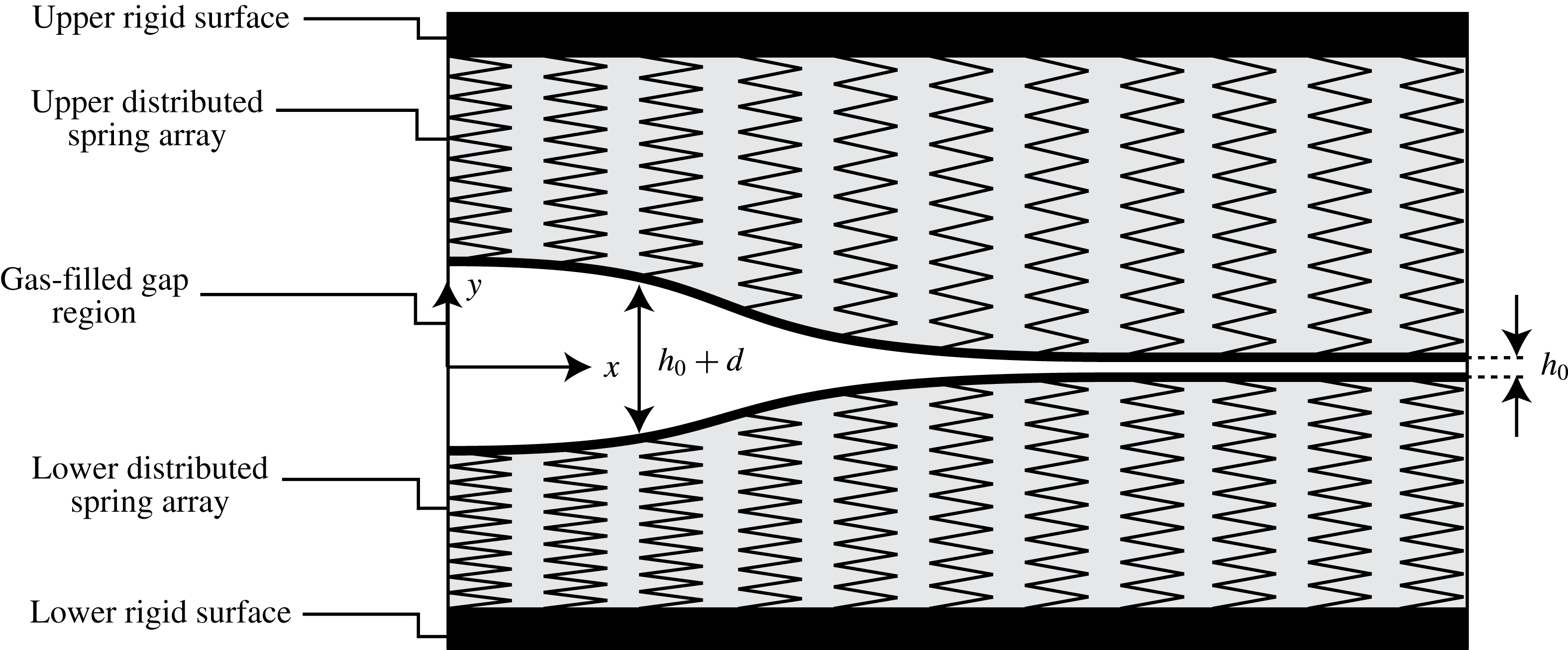
A schematic description of the configuration: a gas-filled gap separates two parallel distributed linear spring arrays bounded by rigid surfaces. The vertical deformation denoted by
 $d$
separates the upper and lower substrates symmetrically about the mid-plane,
 $y=0$
.
2 Problem formulation
We examine pressure-driven gaseous viscous flow in a two-dimensional microchannel bounded by linearly elastic substrates, as illustrated in figure 1. The origin of the
 $(x,y)$
coordinate system is located at the centre of the channel at rest, where
 $x$
is parallel to the channel’s streamwise direction. The axial length scale of the configuration is denoted by
 $l$
, time is
 $t$
and temperature is
 $\unicode[STIX]{x1D703}_{0}$
. The gas velocity vector is defined as
 $\boldsymbol{u}=(u,v)$
, absolute pressure is
 $p$
, the Newtonian stress tensor is
 $\unicode[STIX]{x1D749}$
, gas shear and bulk viscosity coefficients are
 $\unicode[STIX]{x1D707}$
and
 $\unicode[STIX]{x1D6FE}$
, respectively (due to lubrication flow
 $\unicode[STIX]{x1D6FE}$
will be neglected), gas density is
 $\unicode[STIX]{x1D70C}$
, the gas constant is
 ${\mathcal{R}}$
and the gas mean free path is
 $\unicode[STIX]{x1D706}$
. At rest, the constant gap between the lower and upper substrates is denoted by
 $h_{0}$
, and contains gas at background pressure
 $p_{0}$
. The channel height
 $h$
, the pressure-induced vertical deformation
 $d$
, and the pressure
 $p$
are related by
 $$\begin{eqnarray}h=h_{0}+d,\quad p=p_{0}+kd,\end{eqnarray}$$
where
 $k$
is the stiffness of the substrates. The system is assumed to be symmetric about the mid-plane
 $y=0$
; a discussion of the asymmetric case is given in § 5.
The current model only considers vertical displacements, a common assumption in elastic microchannels (e.g. Gervais et al.
Reference Gervais, El-Ali, Günther and Jensen2006; Hardy et al.
Reference Hardy, Uechi, Zhen and Kavehpour2009). Specifically, examining the stress exerted by the fluid on the substrate interface, for slender channels (with aspect ratio
 $\unicode[STIX]{x1D700}\ll 1$
) the shear stress scales with
 $\unicode[STIX]{x1D70E}_{xy}\sim \unicode[STIX]{x1D700}p$
whereas the normal stress scales with
 $\unicode[STIX]{x1D70E}_{yy}\sim p$
. Thus streamwise displacements due to shear stress are negligible. In addition, for slender elastic configurations bound to rigid surfaces (see figure 1, representing practical working configurations such as PDMS bound to glass) the Hookean requirement of small strain limits the streamwise deformation to be small compared with channel length, and the vertical deformation to be small compared with the height of the spring array. The vertical deformation, however, may be large compared with the initial channel thickness
 $h_{0}$
, yet still involve small elastic strains. Given these assumptions, the current model may be used to describe one-dimensional compressible lubrication flow in other elastic settings which employ (2.1). Examples are given in § 5.
Under the assumptions of isothermal flow (see appendix B) and negligible body forces, which are common practice for flows through micron-sized configurations (e.g. Arkilic, Breuer & Schmidt Reference Arkilic, Breuer and Schmidt2001; Zohar et al. Reference Zohar, Lee, Lee, Jiang and Tong2002), we begin by considering the governing equations of motion for a perfect viscous gas. Written in dimensional form are the momentum equation,
 $$\begin{eqnarray}\unicode[STIX]{x1D70C}\left(\frac{\unicode[STIX]{x2202}\boldsymbol{u}}{\unicode[STIX]{x2202}t}+\boldsymbol{u}\boldsymbol{\cdot }\unicode[STIX]{x1D735}\boldsymbol{u}\right)=-\unicode[STIX]{x1D735}p+\unicode[STIX]{x1D735}\boldsymbol{\cdot }\unicode[STIX]{x1D749},\end{eqnarray}$$
the compressible continuity equation,
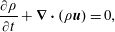 $$\begin{eqnarray}\frac{\unicode[STIX]{x2202}\unicode[STIX]{x1D70C}}{\unicode[STIX]{x2202}t}+\unicode[STIX]{x1D735}\boldsymbol{\cdot }\left(\unicode[STIX]{x1D70C}\boldsymbol{u}\right)=0,\end{eqnarray}$$
and the equation of state,
 $$\begin{eqnarray}p=\unicode[STIX]{x1D70C}{\mathcal{R}}\unicode[STIX]{x1D703}_{0}.\end{eqnarray}$$
The temperature
 $\unicode[STIX]{x1D703}_{0}$
is constant (discussion of the assumption of isothermality is given in appendix B). The stress tensor for a Newtonian gas is given by
 $$\begin{eqnarray}\unicode[STIX]{x1D749}=\unicode[STIX]{x1D707}(\unicode[STIX]{x1D735}\boldsymbol{u}+\unicode[STIX]{x1D735}\boldsymbol{u}^{tr})-({\textstyle \frac{2}{3}}\unicode[STIX]{x1D707}-\unicode[STIX]{x1D6FE})(\unicode[STIX]{x1D735}\boldsymbol{\cdot }\boldsymbol{u})\unicode[STIX]{x1D644}.\end{eqnarray}$$
We define the Knudsen number,
 $Kn$
(a variable in the present problem), as the ratio between the molecular mean free path
 $\unicode[STIX]{x1D706}$
and the local channel height
 $h$
. Its reference value
 $Kn_{0}$
is defined as the ratio of reference mean free path
 $\unicode[STIX]{x1D706}_{0}$
(corresponding to reference pressure
 $p_{0}$
) to initial channel height
 $h_{0}$
. Since the mean free path is inversely proportional to the local pressure,
 $Kn$
takes on the form
 $$\begin{eqnarray}Kn=\frac{\unicode[STIX]{x1D706}}{h}=Kn_{0}\left(\frac{p_{0}}{p}\right)\left(\frac{h_{0}}{h}\right).\end{eqnarray}$$
For the steady cases considered herein
 $Kn_{0}$
expresses the outlet Knudsen number, by analogy to rigid-walled gaseous micro-fluidics. For the transient cases
 $Kn_{0}$
is the Knudsen number ahead of any disturbance where the channel is at rest. The validity of the continuum assumption requires a vanishingly small Knudsen number (practically, as small as
 $Kn<10^{-3}$
); however, for gas flows through micron-sized configurations at standard atmospheric conditions the Knudsen number ranges between
 $Kn\approx 10^{-1}$
and
 $10^{-2}$
. This Knudsen regime requires modification of the continuum model by incorporation of velocity slip on the deforming substrate walls. Thus the boundary conditions for the flow are given by the Navier-slip condition, written in dimensional form as
 $$\begin{eqnarray}u=\mp \unicode[STIX]{x1D70E}\unicode[STIX]{x1D706}\frac{\unicode[STIX]{x2202}u}{\unicode[STIX]{x2202}y}\quad \text{at }y=\pm h/2,\end{eqnarray}$$
where
 $\unicode[STIX]{x1D706}$
varies with
 $p$
according to (2.3), as well as the kinematic boundary condition,
 $$\begin{eqnarray}v=\pm \frac{1}{2}\left(\frac{\unicode[STIX]{x2202}h}{\unicode[STIX]{x2202}t}+u\frac{\unicode[STIX]{x2202}h}{\unicode[STIX]{x2202}x}\right)\quad \text{at }y=\pm h/2,\end{eqnarray}$$
both implemented at the gas–substrate interface. In (2.4a
)
 $\unicode[STIX]{x1D70E}$
denotes the streamwise momentum accommodation coefficient. It is related to the tangential momentum accommodation coefficient
 $\unicode[STIX]{x1D70E}_{m}$
via
 $$\begin{eqnarray}\unicode[STIX]{x1D70E}=\frac{2-\unicode[STIX]{x1D70E}_{m}}{\unicode[STIX]{x1D70E}_{m}},\end{eqnarray}$$
which represents the interaction between the gas molecules and the substrate wall (Chapman & Cowling Reference Chapman and Cowling1952). A value of
 $\unicode[STIX]{x1D70E}_{m}=0$
corresponds to specular reflection (zero accommodation), whereas
 $\unicode[STIX]{x1D70E}_{m}=1$
corresponds to full accommodation which will be the assumed case for the current work, thus in all calculations
 $\unicode[STIX]{x1D70E}=1$
.
3 Derivation of the channel height evolution equation
The displacement of the substrates is assumed to be a linear function of the pressure, hence
 $d^{\ast }=p^{\ast }/k$
may be taken as its characteristic value, where
 $p^{\ast }$
is the characteristic gauge pressure (representing the characteristic value of
 $p-p_{0}$
).
For practical purposes, it is assumed that the characteristic pressure is a known and controlled input parameter in the system, thus the vertical length scale of
 $d^{\ast }$
which enters in the non-dimensionalization (soon to follow) will be replaced by
 $p^{\ast }/k$
where applicable. We hereafter denote normalized variables by capital letters and define the dimensionless ratios
 $$\begin{eqnarray}\unicode[STIX]{x1D6F1}_{H}=\frac{h_{0}k}{p^{\ast }},\quad \unicode[STIX]{x1D6F1}_{P}=\frac{p_{0}}{p^{\ast }},\end{eqnarray}$$
representing the ratio of initial gap to elastic displacements (also termed prewetting thickness ratio) and the ratio of external background pressure to
 $p^{\ast }$
, respectively. The limit
 $\unicode[STIX]{x1D6F1}_{H}\rightarrow \infty$
corresponds to negligible elastic deformations, while the limit
 $\unicode[STIX]{x1D6F1}_{P}\rightarrow \infty$
corresponds to negligible compressibility effects.
Scaling according to the lubrication approximation, the corresponding normalized variables are the coordinates
 $(X,Y)$
, time
 $T$
, vertical displacement
 $D$
, channel height
 $H$
,
 $$\begin{eqnarray}X=\frac{x}{l},\quad Y=\frac{yk}{p^{\ast }},\quad T=\frac{t{p^{\ast }}^{3}}{k^{2}l^{2}\unicode[STIX]{x1D707}},\quad D=\frac{\text{d}k}{p^{\ast }},\quad H=\frac{hk}{p^{\ast }}=\unicode[STIX]{x1D6F1}_{H}+D,\end{eqnarray}$$
fluid velocities
 $(U,V)$
, pressure
 $P$
and density
 $\unicode[STIX]{x1D6EC}$
,
 $$\begin{eqnarray}U=\frac{uk^{2}\unicode[STIX]{x1D707}l}{{p^{\ast }}^{3}},\quad V=\frac{vk^{3}\unicode[STIX]{x1D707}l^{2}}{{p^{\ast }}^{4}},\quad P=\frac{p}{p^{\ast }},\quad \unicode[STIX]{x1D6EC}=\frac{\unicode[STIX]{x1D70C}}{p^{\ast }/{\mathcal{R}}\unicode[STIX]{x1D703}_{0}}.\end{eqnarray}$$
Normalized linear relations between vertical displacement and pressure or alternatively, between channel height and pressure readily follow:
 $$\begin{eqnarray}D=P-\unicode[STIX]{x1D6F1}_{P},\quad H=P+\unicode[STIX]{x1D6F1}_{H}-\unicode[STIX]{x1D6F1}_{P}.\end{eqnarray}$$
Applying the above non-dimensionalizations to (2.2), the requirements for validity of the lubrication approximation are given by the following relations:
 $$\begin{eqnarray}\unicode[STIX]{x1D700}=\frac{p^{\ast }}{kl}\ll 1,\quad \unicode[STIX]{x1D700}Re=\frac{{p^{\ast }}^{6}}{{\mathcal{R}}\unicode[STIX]{x1D703}_{0}k^{4}\unicode[STIX]{x1D707}^{2}l^{2}}\ll 1,\end{eqnarray}$$
where
 $\unicode[STIX]{x1D700}$
represents the slenderness of the configuration and
 $\unicode[STIX]{x1D700}Re$
is the reduced Reynolds number. Consequently, the leading-order balance of the momentum equations (2.2a
) reduces to standard lubrication form,
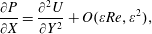 $$\begin{eqnarray}\displaystyle & \displaystyle \frac{\unicode[STIX]{x2202}P}{\unicode[STIX]{x2202}X}=\frac{\unicode[STIX]{x2202}^{2}U}{\unicode[STIX]{x2202}Y^{2}}+O(\unicode[STIX]{x1D700}Re,\unicode[STIX]{x1D700}^{2}), & \displaystyle\end{eqnarray}$$
 $$\begin{eqnarray}\displaystyle & \displaystyle \frac{\unicode[STIX]{x2202}P}{\unicode[STIX]{x2202}Y}=O(\unicode[STIX]{x1D700}^{3}Re,\unicode[STIX]{x1D700}^{2}), & \displaystyle\end{eqnarray}$$
 $$\begin{eqnarray}\frac{\unicode[STIX]{x2202}\unicode[STIX]{x1D6EC}}{\unicode[STIX]{x2202}T}+\frac{\unicode[STIX]{x2202}(\unicode[STIX]{x1D6EC}U)}{\unicode[STIX]{x2202}X}+\frac{\unicode[STIX]{x2202}(\unicode[STIX]{x1D6EC}V)}{\unicode[STIX]{x2202}Y}=0,\end{eqnarray}$$
and
 $$\begin{eqnarray}\unicode[STIX]{x1D6EC}=P,\end{eqnarray}$$
respectively. Pressure may thus be substituted for density throughout. When normalized, the Navier-slip condition (2.4a ) takes the form
 $$\begin{eqnarray}U=\mp \frac{\unicode[STIX]{x1D70E}Kn_{0}\unicode[STIX]{x1D6F1}_{H}\unicode[STIX]{x1D6F1}_{P}}{P}\frac{\unicode[STIX]{x2202}U}{\unicode[STIX]{x2202}Y}\quad \text{at }Y=\pm H/2,\end{eqnarray}$$
while the kinematic boundary condition (2.4b ) reads
 $$\begin{eqnarray}V=\pm \frac{1}{2}\left(\frac{\unicode[STIX]{x2202}H}{\unicode[STIX]{x2202}T}+U\frac{\unicode[STIX]{x2202}H}{\unicode[STIX]{x2202}X}\right)\quad \text{at }Y=\pm H/2.\end{eqnarray}$$
The resulting normalized slip length in (3.9a
) stems from the definition of the Knudsen number (see 2.3) and reflects the choice of
 $h_{0}$
as the reference height for
 $Kn_{0}$
and
 $p^{\ast }/k$
as the scale of the vertical coordinate
 $y$
. The formulated peeling problem has two sources of time evolution. The first comes from the kinematic condition (3.9b
) while the second comes from the unsteady mass conservation equation (3.7). It will be shown in the following sections that many of the properties of the solution will be determined by a competition between these two mechanisms.
Applying (3.9a
) to the
 $X$
-momentum equation (3.6a
) yields the velocity profile
 $$\begin{eqnarray}U=\frac{1}{2}\frac{\unicode[STIX]{x2202}P}{\unicode[STIX]{x2202}X}\left(Y^{2}-\frac{H^{2}}{4}-\unicode[STIX]{x1D70E}Kn_{0}\unicode[STIX]{x1D6F1}_{H}\unicode[STIX]{x1D6F1}_{P}\frac{H}{P}\right).\end{eqnarray}$$
Integration of the continuity equation with respect to
 $Y$
across the gas layer and in conjunction with (3.9b
)–(3.10) yields the following evolution equation, relating channel height
 $H$
, pressure
 $P$
and density
 $\unicode[STIX]{x1D6EC}$
,
 $$\begin{eqnarray}\frac{\unicode[STIX]{x2202}(\unicode[STIX]{x1D6EC}H)}{\unicode[STIX]{x2202}T}=\frac{\unicode[STIX]{x2202}}{\unicode[STIX]{x2202}X}\left\{\left(\frac{H^{3}}{12}+\frac{\unicode[STIX]{x1D70E}Kn_{0}\unicode[STIX]{x1D6F1}_{H}\unicode[STIX]{x1D6F1}_{P}}{2}\frac{H^{2}}{P}\right)\frac{\unicode[STIX]{x2202}P}{\unicode[STIX]{x2202}X}\unicode[STIX]{x1D6EC}\right\},\end{eqnarray}$$
which describes conservation of mass as gaseous viscous flow is driven by a pressure gradient down the compliant-walled channel, where the diffusion coefficient is given by the classical lubrication term
 $H^{3}/12$
as well as a term arising from Navier slip, associated with rarefaction effects. Elastic effects, i.e. variations in channel height
 $H$
due to changes in pressure, are negligible when
 $D\ll \unicode[STIX]{x1D6F1}_{H}$
(i.e.
 $d\ll h_{0}$
). Compressibility effects, i.e. variations in density
 $\unicode[STIX]{x1D6EC}$
, are negligible when
 $D\ll \unicode[STIX]{x1D6F1}_{P}$
(i.e.
 $d\ll p_{0}/k$
). Rarefaction effects are negligible when
 $HP\gg \unicode[STIX]{x1D70E}Kn_{0}\unicode[STIX]{x1D6F1}_{H}\unicode[STIX]{x1D6F1}_{P}$
. Finally, a governing equation for the channel height
 $H$
may be attained by incorporating the linear relation between pressure and channel height (3.4), and rearranging,
 $$\begin{eqnarray}\frac{\unicode[STIX]{x2202}H}{\unicode[STIX]{x2202}{\mathcal{T}}}=\frac{1}{2H+\unicode[STIX]{x1D6F1}_{P}-\unicode[STIX]{x1D6F1}_{H}}\frac{\unicode[STIX]{x2202}}{\unicode[STIX]{x2202}X}\left\{[H^{3}(H+\unicode[STIX]{x1D6F1}_{P}-\unicode[STIX]{x1D6F1}_{H})+6\unicode[STIX]{x1D70E}Kn_{0}\unicode[STIX]{x1D6F1}_{H}\unicode[STIX]{x1D6F1}_{P}H^{2}]\frac{\unicode[STIX]{x2202}H}{\unicode[STIX]{x2202}X}\right\},\end{eqnarray}$$
where hereafter
 ${\mathcal{T}}=T/12$
for convenience. Equation (3.12) is given in its dimensional form in (A 1). For some of the cases considered herein it is worthwhile to represent (3.12) in the deflection variable
 $D$
, which reads
 $$\begin{eqnarray}\frac{\unicode[STIX]{x2202}D}{\unicode[STIX]{x2202}{\mathcal{T}}}=\frac{1}{2D+\unicode[STIX]{x1D6F1}_{P}+\unicode[STIX]{x1D6F1}_{H}}\frac{\unicode[STIX]{x2202}}{\unicode[STIX]{x2202}X}\left\{[(D+\unicode[STIX]{x1D6F1}_{P})(D+\unicode[STIX]{x1D6F1}_{H})^{3}+6\unicode[STIX]{x1D70E}Kn_{0}\unicode[STIX]{x1D6F1}_{H}\unicode[STIX]{x1D6F1}_{P}(D+\unicode[STIX]{x1D6F1}_{H})^{2}]\frac{\unicode[STIX]{x2202}D}{\unicode[STIX]{x2202}X}\right\},\end{eqnarray}$$
and may be convenient due to homogeneous boundary conditions.
4 Solutions of the evolution equation
4.1 Steady state
We start our analysis of the governing equation (3.12) by examining its steady-state ordinary differential equation (ODE) form in the pressure variable
 $$\begin{eqnarray}\frac{\text{d}}{\text{d}X}\left\{[P(P+\unicode[STIX]{x1D6F1}_{H}-\unicode[STIX]{x1D6F1}_{P})^{3}+6\unicode[STIX]{x1D70E}Kn_{0}\unicode[STIX]{x1D6F1}_{H}\unicode[STIX]{x1D6F1}_{P}(P+\unicode[STIX]{x1D6F1}_{H}-\unicode[STIX]{x1D6F1}_{P})^{2}]\frac{\text{d}P}{\text{d}X}\right\}=0.\end{eqnarray}$$
We first note that by taking the limit
 $\unicode[STIX]{x1D6F1}_{H}\rightarrow \infty$
in (4.1) and neglecting elastic deformations, we recover the governing equation for the leading-order pressure distribution of a two-dimensional rigid microchannel (Arkilic et al.
Reference Arkilic, Schmidt and Breuer1997),
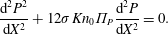 $$\begin{eqnarray}\frac{\text{d}^{2}P^{2}}{\text{d}X^{2}}+12\unicode[STIX]{x1D70E}Kn_{0}\unicode[STIX]{x1D6F1}_{P}\frac{\text{d}^{2}P}{\text{d}X^{2}}=0.\end{eqnarray}$$
Unlike the rigid case, which has an exact explicit solution, the more general elastic case can only be solved implicitly. Assuming a finite configuration with prescribed pressures at the inlet and outlet sections (
 $P(X=0)$
and
 $P(X=1)$
, respectively) integration of (4.1) yields
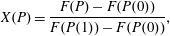 $$\begin{eqnarray}X(P)=\frac{F(P)-F(P(0))}{F(P(1))-F(P(0))},\end{eqnarray}$$
where
 $$\begin{eqnarray}F(P)=40\unicode[STIX]{x1D70E}Kn_{0}\unicode[STIX]{x1D6F1}_{H}\unicode[STIX]{x1D6F1}_{P}(P+\unicode[STIX]{x1D6E5}_{\unicode[STIX]{x1D6F1}})^{3}+5P(P+\unicode[STIX]{x1D6E5}_{\unicode[STIX]{x1D6F1}})^{4}-(P+\unicode[STIX]{x1D6E5}_{\unicode[STIX]{x1D6F1}})^{5},\end{eqnarray}$$
and
 $$\begin{eqnarray}\unicode[STIX]{x1D6E5}_{\unicode[STIX]{x1D6F1}}\equiv \unicode[STIX]{x1D6F1}_{H}-\unicode[STIX]{x1D6F1}_{P}.\end{eqnarray}$$
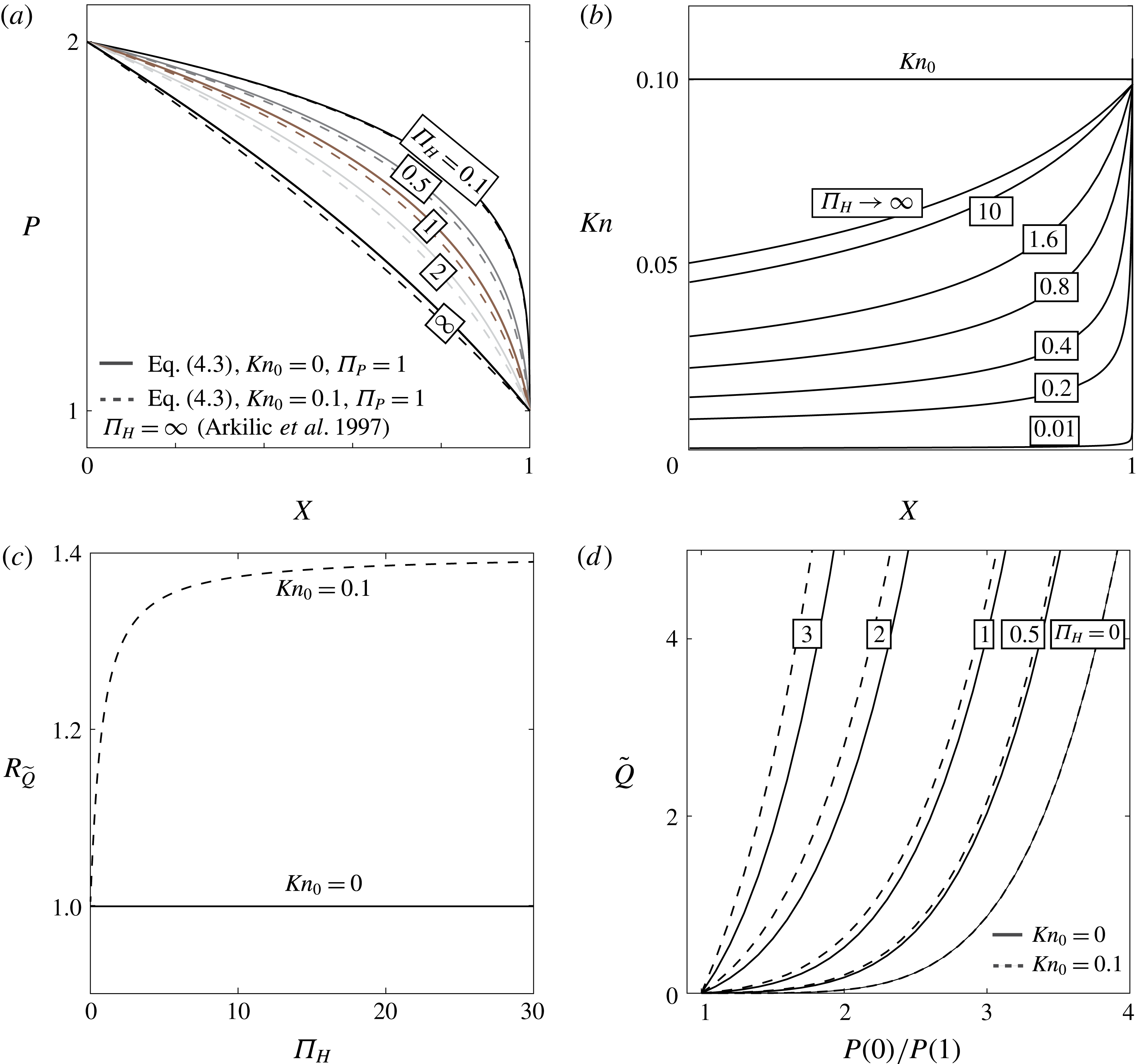
Solution (4.3) is depicted in figure 2(a) for the case of
 $\unicode[STIX]{x1D6F1}_{P}=1$
,
 $P(0)/P(1)=2$
,
 $Kn_{0}=0$
(solid lines) and
 $Kn_{0}=0.1$
(dashed lines) for various values of
 $\unicode[STIX]{x1D6F1}_{H}$
. The rigid pressure distributions
 $\unicode[STIX]{x1D6F1}_{H}\rightarrow \infty$
(for both slip and no-slip flow) converge to the solution of (4.2) and have the least curvature (innermost). Smaller values of
 $\unicode[STIX]{x1D6F1}_{H}$
represent larger ratios of elastic deformation to initial channel height
 $h_{0}$
, which reduce the pressure gradient near the inlet while increasing it towards the outlet. For constant initial channel thickness and background pressure (i.e. constant
 $Kn_{0}$
), decreasing
 $\unicode[STIX]{x1D6F1}_{H}$
decreases the local Knudsen number (as seen in figure 2
b) thus decreasing the effect of rarefaction on the pressure distribution. Figure 2(c) presents the effect of rarefaction on the mass flow rate versus
 $\unicode[STIX]{x1D6F1}_{H}$
. The ratio of non-dimensional flow rate for the case of velocity slip over the no-slip flow rate
 $\widetilde{Q}(Kn_{0}=0.1)/\widetilde{Q}(Kn_{0}=0)$
is presented, where
 $\widetilde{Q}=2\int _{0}^{H/2}\unicode[STIX]{x1D6EC}U\,\text{d}Y$
. Rarefaction effects on the mass flow rate tend to a constant finite value for
 $\unicode[STIX]{x1D6F1}_{H}\rightarrow \infty$
, and decrease with
 $\unicode[STIX]{x1D6F1}_{H}$
. Figure 2(d) presents the mass flow rate
 $\widetilde{Q}$
versus the pressure difference for various values of
 $\unicode[STIX]{x1D6F1}_{H}$
. While the gradients of the different lines vary significantly with
 $\unicode[STIX]{x1D6F1}_{H}$
for the limit of small pressures at the inlet, as the inlet pressure increases the viscous resistance no longer depends on
 $\unicode[STIX]{x1D6F1}_{H}$
(or
 $h_{0}$
) and the gradients converge.
Steady-state solution (4.3) of gaseous viscous flow in a two-dimensional microchannel bounded by linearly elastic substrates. Gas pressure (a) and local Knudsen (b) profiles versus
 $X$
for varying
 $\unicode[STIX]{x1D6F1}_{H}$
and
 $P(0)/P(1)=2$
. (c) Ratio of mass flow rates
 $R_{\widetilde{Q}}$
versus
 $\unicode[STIX]{x1D6F1}_{H}$
,
 $R_{\widetilde{Q}}=\widetilde{Q}(Kn_{0})/\widetilde{Q}(Kn_{0}=0)$
,
 $Kn_{0}=0.1$
(dashed),
 $Kn_{0}=0$
(solid),
 $P(0)/P(1)=2$
. (d) Mass flow rate versus pressure ratio
 $P(X=0)/P(X=1)$
for various values of
 $\unicode[STIX]{x1D6F1}_{H}$
. For all panels
 $\unicode[STIX]{x1D70E}=1$
and
 $\unicode[STIX]{x1D6F1}_{P}=1$
. A value of
 $Kn_{0}=0.1$
was used in (b).
Explicit solutions of (4.3) may be obtained for various physical limits involving
 $\unicode[STIX]{x1D6F1}_{P}$
,
 $\unicode[STIX]{x1D6F1}_{H}$
and the deformation variable
 $D$
for the case of negligible slip
 $Kn_{0}\rightarrow 0$
. These can be written as
 $$\begin{eqnarray}D(X)=[((D(1)+C)^{N}-(D(0)+C)^{N})X+(D(0)+C)^{N}]^{1/N}-C,\end{eqnarray}$$
where
 $(N,C)=(5,\unicode[STIX]{x1D6F1}_{P})$
for the limit of
 $\unicode[STIX]{x1D6F1}_{P},\unicode[STIX]{x1D6F1}_{H}\ll D$
or the symmetric case of
 $\unicode[STIX]{x1D6F1}_{P}=\unicode[STIX]{x1D6F1}_{H}$
, representing a compressibility–elasticity–viscosity regime,
 $(N,C)=(2,\unicode[STIX]{x1D6F1}_{P})$
for the limit of
 $\unicode[STIX]{x1D6F1}_{H}\gg \unicode[STIX]{x1D6F1}_{P},D$
(compressibility–viscosity regime),
 $(N,C)=(4,\unicode[STIX]{x1D6F1}_{H})$
for the limit of
 $\unicode[STIX]{x1D6F1}_{P}\gg \unicode[STIX]{x1D6F1}_{H},D$
(elasticity–viscosity regime), and finally,
 $(N,C)=(1,0)$
for the linear limit of
 $\unicode[STIX]{x1D6F1}_{P},\unicode[STIX]{x1D6F1}_{H}\gg D$
(viscous regime).
4.2 Self-similar Barenblatt solutions for negligible rarefaction effects
While exact solutions of (3.12) are not available, several limits involving negligible rarefaction effects yield known self-similar solutions. Furthermore, for a given set of parameters (namely, initial channel height
 $h_{0}$
, substrate stiffness
 $k$
and background pressure
 $p_{0}$
) the flow field may be described by transition in time between different approximate solutions associated with different time scales. Physical insight may thus be gained by mapping the different approximate solutions, their corresponding time scales and the transitions between them.
We focus on fundamental solutions for the case of impulse-driven peeling – an abrupt release of a finite mass
 $M$
(non-dimensional) at
 ${\mathcal{T}}=0$
into the inlet at
 $X=0$
. The integral expressing mass conservation is
 $$\begin{eqnarray}M=\int _{0}^{\infty }[\unicode[STIX]{x1D6EC}H-\unicode[STIX]{x1D6F1}_{H}\unicode[STIX]{x1D6F1}_{P}]\,\text{d}X=\int _{0}^{\infty }[D^{2}+(\unicode[STIX]{x1D6F1}_{H}+\unicode[STIX]{x1D6F1}_{P})D]\,\text{d}X.\end{eqnarray}$$
The boundary conditions are
 $D\rightarrow 0$
as
 $X\rightarrow \infty$
(far-field attenuation, equivalently expressed by
 $P\rightarrow \unicode[STIX]{x1D6F1}_{P}$
or
 $H\rightarrow \unicode[STIX]{x1D6F1}_{H}$
) and
 $\unicode[STIX]{x2202}D/\unicode[STIX]{x2202}X=0$
at
 $X=0$
(no further inlet flux after the initial injection). For some of the cases considered herein the leading-order solutions of (3.13) will exhibit compact support and a distinct propagation front,
 $X=X_{F}({\mathcal{T}})$
. For those cases, the far-field attenuation condition is met exactly at the front and the upper bound of the mass conservation integral (4.5) may be replaced by
 $X=X_{F}$
. The dimensional form of the mass is
 $m=({p^{\ast }}^{2}lw/k{\mathcal{R}}\unicode[STIX]{x1D703}_{0})M$
, where
 $w$
is a lateral dimension, normal to the
 $(x,y)$
plane. We note that from a mathematical standpoint two out of the three parameters
 $\unicode[STIX]{x1D6F1}_{H},\unicode[STIX]{x1D6F1}_{P}$
and
 $M$
can be eliminated in the idealized self-similar problem, since both the height and length scales,
 $d^{\ast }$
and
 $l$
, are arbitrary. However, these parameters are retained due to practical considerations.
4.2.1 Early times
 $D\gg \unicode[STIX]{x1D6F1}_{H}$
,
$\unicode[STIX]{x1D6F1}_{P}$


For sufficiently early times
 $D\gg \unicode[STIX]{x1D6F1}_{H},\unicode[STIX]{x1D6F1}_{P}$
and both elasticity and compressibility contribute to the peeling process. The leading order of equation (3.13) reduces to a porous medium equation (PME) of order
 $2.5$
for the variable
 $Q=D^{2}$
. The corresponding leading-order mass conservation integral (4.5) can also be expressed in terms of
 $Q$
:
 $$\begin{eqnarray}\frac{\unicode[STIX]{x2202}Q}{\unicode[STIX]{x2202}{\mathcal{T}}}=\frac{1}{5}\frac{\unicode[STIX]{x2202}^{2}Q^{2.5}}{\unicode[STIX]{x2202}X^{2}},\quad M=\int _{0}^{X_{F}}Q\,\text{d}X.\end{eqnarray}$$
The initial condition is given by
 $Q(X,{\mathcal{T}}=0)=M\unicode[STIX]{x1D6FF}(X)$
, where
 $\unicode[STIX]{x1D6FF}$
is Dirac’s delta function. Applying Zel’dovich, Kompaneets and Barenblatt’s (ZKB) solution (Barenblatt Reference Barenblatt1952) yields the time propagation rate of
 $X_{F}=O({\mathcal{T}}^{2/7})$
and the peeling dynamics are given by
 $$\begin{eqnarray}D(X,{\mathcal{T}})=0.9659M^{2/7}{\mathcal{T}}^{-1/7}\left[1-\left(\frac{X}{1.45M^{3/7}{\mathcal{T}}^{2/7}}\right)^{2}\right]_{+}^{1/3},\end{eqnarray}$$
where
 $(s)_{_{+}}=\max (s,0)$
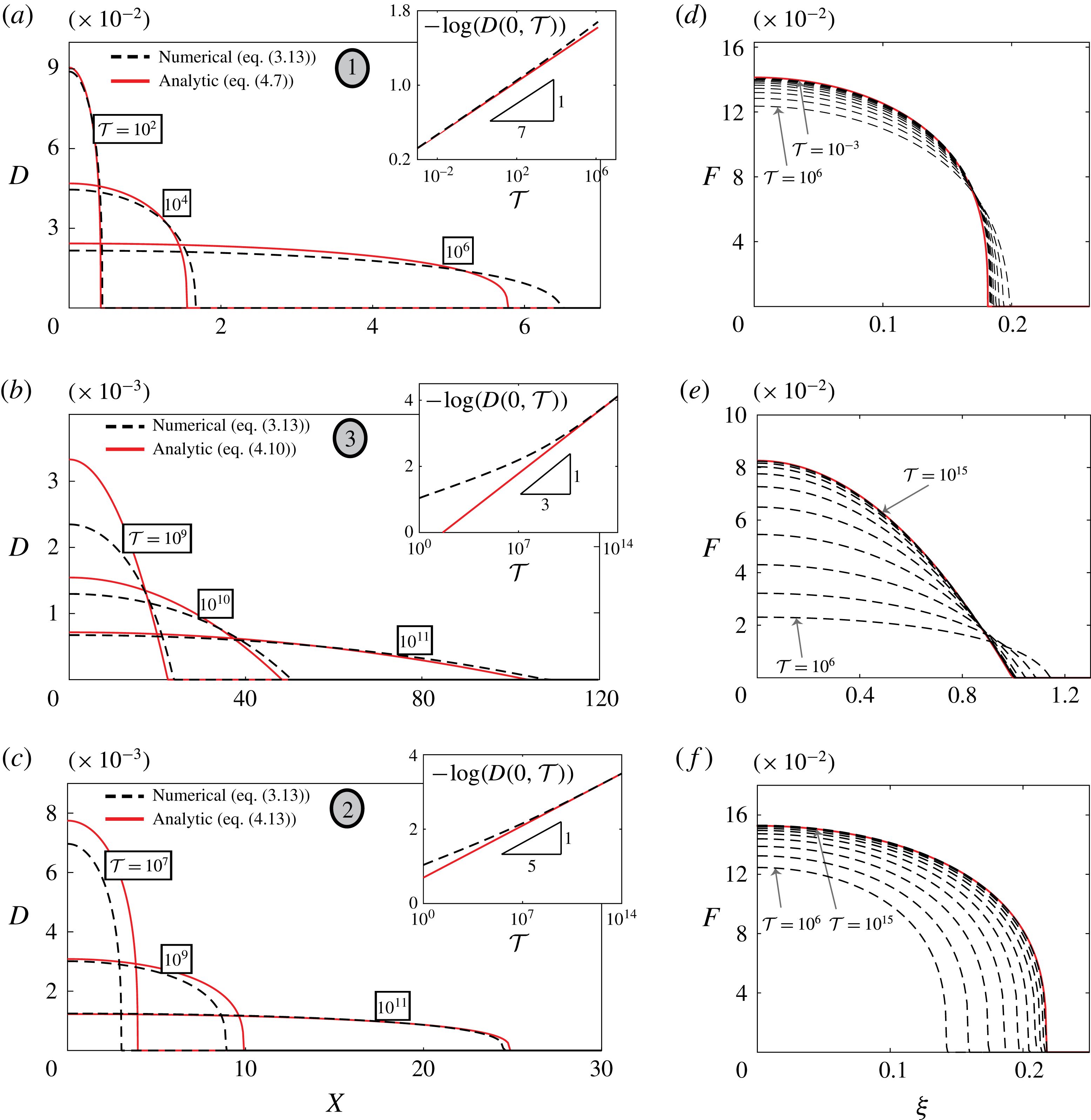
. Solution (4.7) is characterized by a compactly supported region of displacement associated with the peeling process. The solution is given in its dimensional form in (A 3). The convergence of the full numerical solution of (3.13) to the early-time approximation (4.7) is shown in figure 3(a,d). Time snapshots are provided in figure 3(a) along with the maximal channel height (figure 3
a inset) plotted on a double-logarithmic scale. Figure 3(d) illustrates the convergence in the similarity variables
 $D(X,{\mathcal{T}})=((1/5){\mathcal{T}})^{-1/7}F(\unicode[STIX]{x1D709})$
, where
 $\unicode[STIX]{x1D709}=X((1/5){\mathcal{T}})^{-2/7}$
. The numerical deformation profiles obtained from time-stepping over multiple decades were superimposed on the similarity grid. Calculations were performed using a MATLAB-based nonlinear parabolic partial differential equation (PDE) solver. An important property of the solution, as can be seen in figure 3(a), is that its global volume increases with time (for finite mass),
 $\int _{0}^{X_{F}}D(X,{\mathcal{T}})\,\text{d}X=O({\mathcal{T}}^{1/7})$
, a direct consequence of the compressibility–elasticity coupling. As the added mass propagates and expands into the channel, the gas pressure decreases and thus
 $D$
decreases, eventually invalidating the requirement that
 $D\gg \unicode[STIX]{x1D6F1}_{H},\unicode[STIX]{x1D6F1}_{P}$
. This sets a validity time range of (also given in dimensional form in (A 4))
 $$\begin{eqnarray}{\mathcal{T}}\ll \frac{M^{2}}{\max (\unicode[STIX]{x1D6F1}_{H}^{7},\unicode[STIX]{x1D6F1}_{P}^{7})}\end{eqnarray}$$
for (4.7) based on
 $D(X=0,{\mathcal{T}})$
.
Convergence of the numerical deformation profiles obtained from (3.13) to the theoretical results (4.7), (4.10) and (4.13). (a,d) Compressibility–elasticity–viscosity regime (transitioning towards compressibility–viscosity regime),
 $(M,\unicode[STIX]{x1D6F1}_{H},\unicode[STIX]{x1D6F1}_{P})=(2.77\times 10^{-4},5\times 10^{-3},0)$
. (b,e) Compressibility–viscosity regime (approaching from compressibility–elasticity–viscosity regime),
 $(M,\unicode[STIX]{x1D6F1}_{H},\unicode[STIX]{x1D6F1}_{P})$
the same as above. (c,f) Elasticity–viscosity regime (approaching from compressibility–elasticity–viscosity regime),
 $(M,\unicode[STIX]{x1D6F1}_{H},\unicode[STIX]{x1D6F1}_{P})=(2.86\times 10^{-4},0,1\times 10^{-2})$
. Panels (a), (b) and (c), respectively, present time snapshot comparisons over several decades and include insets of the maximal deflection (double-logarithmic scale). Panels (d), (e) and (f), respectively, depict the convergence in the similarity variables
 $(\unicode[STIX]{x1D709},F)$
. The numerical deformation profiles obtained from time-stepping were superimposed on the similarity grid, 10 consecutive decades are shown in each case. The values of (
 $M,\unicode[STIX]{x1D6F1}_{H},\unicode[STIX]{x1D6F1}_{P}$
) used here correspond to those used in the simulations which will follow in figure 5. In panels (a), (b) and (c) the grey ellipse numbering scheme defined in figure 4 is used to label the regimes.
4.2.2 Intermediate times
$\unicode[STIX]{x1D6F1}_{P}\ll D\ll \unicode[STIX]{x1D6F1}_{H}$
or
$\unicode[STIX]{x1D6F1}_{H}\ll D\ll \unicode[STIX]{x1D6F1}_{P}$


Beyond the range of (4.8) the solution may branch into one of two regimes, contingent upon the ratio of
 $\unicode[STIX]{x1D6F1}_{H}/\unicode[STIX]{x1D6F1}_{P}$
. If the ratio is significantly larger than unity
 $\unicode[STIX]{x1D6F1}_{H}/\unicode[STIX]{x1D6F1}_{P}=h_{0}/(p_{0}/k)\gg 1$
(corresponding to negligible effects of elasticity and dominant effects of gas compressibility) an intermediate regime exists where
 $\unicode[STIX]{x1D6F1}_{P}\ll D\ll \unicode[STIX]{x1D6F1}_{H}$
. In this regime, the leading order of equation (3.13) is a porous medium equation of order 2 for
 $D$
; the leading-order mass integral (4.5) reduces to volume conserving form,
 $$\begin{eqnarray}\frac{\unicode[STIX]{x2202}D}{\unicode[STIX]{x2202}{\mathcal{T}}}=\frac{\unicode[STIX]{x1D6F1}_{H}^{2}}{2}\frac{\unicode[STIX]{x2202}^{2}D^{2}}{\unicode[STIX]{x2202}X^{2}},\quad M=\unicode[STIX]{x1D6F1}_{H}\int _{0}^{X_{F}}D\,\text{d}X.\end{eqnarray}$$
The solution will thus transition to a propagation rate of
 $X_{F}=O({\mathcal{T}}^{1/3})$
and the resulting profile
 $$\begin{eqnarray}D(X,{\mathcal{T}})=0.7211M^{2/3}\unicode[STIX]{x1D6F1}_{H}^{-4/3}{\mathcal{T}}^{-1/3}\left[1-\left(\frac{X}{2.0801M^{1/3}\unicode[STIX]{x1D6F1}_{H}^{1/3}{\mathcal{T}}^{1/3}}\right)^{2}\right]_{+}\end{eqnarray}$$
will emerge in intermediate times with a validity range of
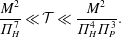 $$\begin{eqnarray}\frac{M^{2}}{\unicode[STIX]{x1D6F1}_{H}^{7}}\ll {\mathcal{T}}\ll \frac{M^{2}}{\unicode[STIX]{x1D6F1}_{H}^{4}\unicode[STIX]{x1D6F1}_{P}^{3}}.\end{eqnarray}$$
See (A 5) and (A 6) for the dimensional forms of (4.10) and (4.11), respectively. Solution (4.10) represents the limit of dominant gas compressibility, and is identical to the evolution of compressible low-Reynolds-number gas flow in rigid configurations and analogous to ideal isothermal gas flow in a homogeneous porous medium (Leibenzon Reference Leibenzon1930; Muskat Reference Muskat1937). The relevant time scale of this limit is
 $t\sim \unicode[STIX]{x1D707}/p^{\ast }(h_{0}/l)^{2}$
. Convergence of the numerical solution of (3.13) to the intermediate-time profiles (4.10) for the case of
 $\unicode[STIX]{x1D6F1}_{H}/\unicode[STIX]{x1D6F1}_{P}\gg 1$
is shown in figure 3(b,e). Time snapshots are provided in figure 3(b) along with the maximal value of
 $D$
at the base (figure 3
b inset). Figure 3(e) depicts the convergence of superimposed numerical profiles when collapsed on the self-similar grid using the transformation
 $D(X,{\mathcal{T}})=((\unicode[STIX]{x1D6F1}_{H}^{2}/2){\mathcal{T}})^{-1/3}F(\unicode[STIX]{x1D709})$
, where
 $\unicode[STIX]{x1D709}=X((\unicode[STIX]{x1D6F1}_{H}^{2}/2){\mathcal{T}})^{-1/3}$
.
Alternatively, for
 $\unicode[STIX]{x1D6F1}_{P}/\unicode[STIX]{x1D6F1}_{H}=p_{0}/kh_{0}\gg 1$
, a different intermediate regime exists for which
 $\unicode[STIX]{x1D6F1}_{H}\ll D\ll \unicode[STIX]{x1D6F1}_{P}$
. The leading-order evolution equation is a porous medium equation of order 4 for
 $D$
, while (4.5) takes on an alternate volume conserving form,
 $$\begin{eqnarray}\frac{\unicode[STIX]{x2202}D}{\unicode[STIX]{x2202}{\mathcal{T}}}=\frac{1}{4}\frac{\unicode[STIX]{x2202}^{2}D^{4}}{\unicode[STIX]{x2202}X^{2}},\quad M=\unicode[STIX]{x1D6F1}_{P}\int _{0}^{X_{F}}D\,\text{d}X,\end{eqnarray}$$
yielding
 $$\begin{eqnarray}D(X,{\mathcal{T}})=0.8423M^{2/5}\unicode[STIX]{x1D6F1}_{P}^{-2/5}{\mathcal{T}}^{-1/5}\left[1-\left(\frac{X}{1.4112M^{3/5}\unicode[STIX]{x1D6F1}_{P}^{-3/5}{\mathcal{T}}^{1/5}}\right)^{2}\right]_{_{+}}^{1/3}\end{eqnarray}$$
with an
 $X_{F}=O({\mathcal{T}}^{1/5})$
spread rate, typical of the early-time propagation of the incompressible peeling problem (e.g. Elbaz & Gat Reference Elbaz and Gat2016), and a validity range of
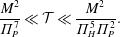 $$\begin{eqnarray}\frac{M^{2}}{\unicode[STIX]{x1D6F1}_{P}^{7}}\ll {\mathcal{T}}\ll \frac{M^{2}}{\unicode[STIX]{x1D6F1}_{H}^{5}\unicode[STIX]{x1D6F1}_{P}^{2}}.\end{eqnarray}$$
See (A 7) and (A 8) for the dimensional forms of (4.13) and (4.14), respectively. Convergence of the numerical solution of (3.13) to the alternative intermediate-time profiles (4.13) for the case of
 $\unicode[STIX]{x1D6F1}_{P}/\unicode[STIX]{x1D6F1}_{H}\gg 1$
is shown in figure 3(c,f). Time snapshots are provided in figure 3(c) along with the maximal channel deflection (figure 3
c inset). Figure 3(f) depicts the convergence of superimposed numerical profiles when collapsed on the self-similar grid. The relevant transformation for the current case is
 $D(X,{\mathcal{T}})=((1/4){\mathcal{T}})^{-1/5}F(\unicode[STIX]{x1D709})$
, where
 $\unicode[STIX]{x1D709}=X((1/4){\mathcal{T}})^{-1/5}$
.
We note that the asymptotic ZKB solutions presented thus far fail to capture the physical boundary condition ahead of the front which must require some form of regularization. From a numerical standpoint this is achieved by reintroducing small values of
 $(\unicode[STIX]{x1D6F1}_{H},\unicode[STIX]{x1D6F1}_{P})$
as performed presently. This can also be done analytically by matching the ZKB solutions, which are valid in the bulk outside the front, to an exponential solution near the front which decays in the far field. The process was addressed by the authors in a related problem (see Elbaz & Gat Reference Elbaz and Gat2016).
4.2.3 Late times
$D\ll \unicode[STIX]{x1D6F1}_{H},\unicode[STIX]{x1D6F1}_{P}$

All solutions will ultimately settle on the late-time behaviour of
 $X_{F}=O({\mathcal{T}}^{1/2})$
as
 ${\mathcal{T}}\rightarrow \infty$
whether it is the prewetting thickness ratio
 $\unicode[STIX]{x1D6F1}_{H}$
or the background to gauge pressure ratio
 $\unicode[STIX]{x1D6F1}_{P}$
that is the final regularization mechanism which linearizes (3.13). For such late times propagation is governed by the linear heat equation,
 $$\begin{eqnarray}\frac{\unicode[STIX]{x2202}D}{\unicode[STIX]{x2202}{\mathcal{T}}}=\frac{\unicode[STIX]{x1D6F1}_{H}^{3}(1+6\unicode[STIX]{x1D70E}Kn_{0})}{1+\unicode[STIX]{x1D6F1}_{H}/\unicode[STIX]{x1D6F1}_{P}}\frac{\unicode[STIX]{x2202}^{2}D}{\unicode[STIX]{x2202}X^{2}},\end{eqnarray}$$
with corresponding fundamental solution,
 $$\begin{eqnarray}D(X,{\mathcal{T}})=\frac{M}{\sqrt{\unicode[STIX]{x1D70B}(\unicode[STIX]{x1D6F1}_{H}+\unicode[STIX]{x1D6F1}_{P})\unicode[STIX]{x1D6F1}_{P}\unicode[STIX]{x1D6F1}_{H}^{3}(1+6\unicode[STIX]{x1D70E}Kn_{0}){\mathcal{T}}}}\exp \left\{-\frac{(1+\unicode[STIX]{x1D6F1}_{H}/\unicode[STIX]{x1D6F1}_{P})X^{2}}{4\unicode[STIX]{x1D6F1}_{H}^{3}(1+6\unicode[STIX]{x1D70E}Kn_{0}){\mathcal{T}}}\right\},\end{eqnarray}$$
and range of validity,
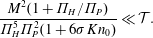 $$\begin{eqnarray}\frac{M^{2}(1+\unicode[STIX]{x1D6F1}_{H}/\unicode[STIX]{x1D6F1}_{P})}{\unicode[STIX]{x1D6F1}_{H}^{5}\unicode[STIX]{x1D6F1}_{P}^{2}(1+6\unicode[STIX]{x1D70E}Kn_{0})}\ll {\mathcal{T}}.\end{eqnarray}$$
See (A 9) and (A 10) for the dimensional forms of (4.16) and (4.17), respectively. Velocity slip is shown to accelerate the propagation causing the system to linearize sooner (this point will be illustrated numerically in § 4.3).
Finally, we note that while the analytical treatment of § 4.2 is of an idealized impulsive mass insertion, in a more realistic setting where the mass is introduced over a non-zero time scale
 ${\mathcal{T}}_{0}$
, a regime which is only valid for
 ${\mathcal{T}}\ll {\mathcal{T}}_{0}$
will be skipped and not observed.
4.3 Numerical validation of regime transitions
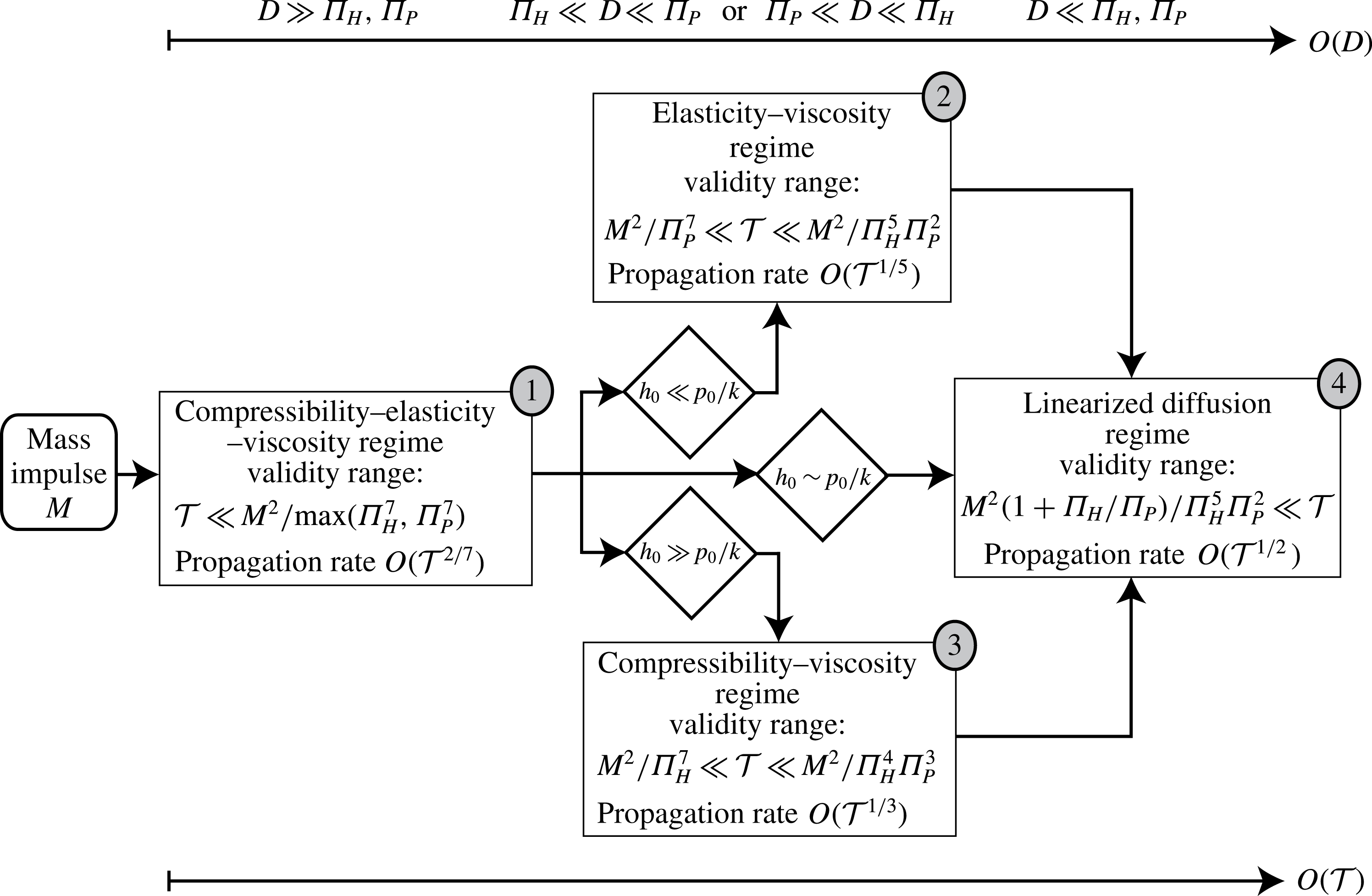
We first illustrate the regime transitions discussed in §§ 4.2.1, 4.2.2 and 4.2.3 in the flow chart shown in figure 4. It is initiated by an impulsive mass insertion of magnitude
 $M$
and flows temporally from left to right. The dominant balances of equation (3.13) associated with each regime are shown in the top order-of-magnitude axis of the deflection
 $D$
in sequence. The regimes are labelled
 $(1),\ldots ,(4)$
in grey ellipses. The corresponding time ranges for each temporal limit are also presented in the figure and were calculated by requiring the appropriate order of magnitude of
 $D$
for the examined limit from solutions (4.7), (4.10) and (4.13) at
 $X=0$
. Non-dimensional parametric conditions involving
 $(\unicode[STIX]{x1D6F1}_{H},\unicode[STIX]{x1D6F1}_{P})$
are stated in dimensional form (diamonds) in terms of the initial channel thickness
 $h_{0}$
, channel stiffness
 $k$
and background pressure
 $p_{0}$
.
For the numerical simulation of regime transitions we chose the initial value of
 $D(X=0,{\mathcal{T}}\rightarrow 0)\sim 1$
which defines the characteristic deflection
 $d^{\ast }=d(x=0,t\rightarrow 0)$
and sets the requirement that
 $\unicode[STIX]{x1D6F1}_{H},\unicode[STIX]{x1D6F1}_{P}\ll 1$
for the appearance of the early-time regime (i.e. large actuation gauge pressure compared with the background pressure and large displacement to prewetting thickness ratio). The initial volume
 $\int _{0}^{\infty }D(X,0)\,\text{d}X$
was set constant for all numerical runs. Consequently, the value of
 $M$
, calculated from (4.5), is kept constant as
 $(\unicode[STIX]{x1D6F1}_{H},\unicode[STIX]{x1D6F1}_{P})$
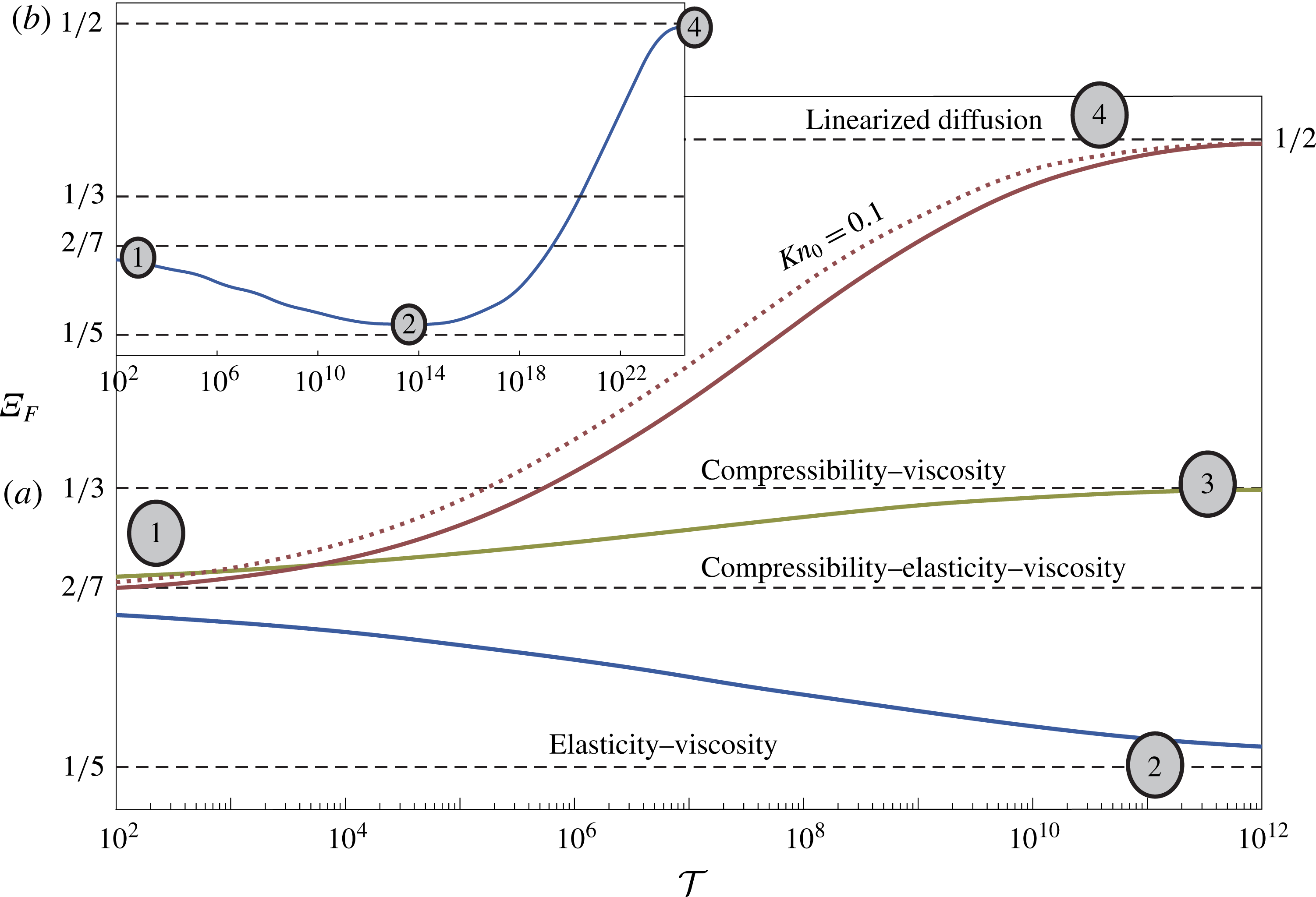
are varied between simulations but maintained small. The evolution of the solution through the various regimes is presented in figures 3 and 5. The solution
 $D(X,{\mathcal{T}})$
was first computed from (3.13). The logarithmic derivative of the peeling front location
 $X_{F}({\mathcal{T}})$
was then calculated,
 $\unicode[STIX]{x1D6EF}_{F}\equiv \text{d}(\log X_{F})/\text{d}(\log {\mathcal{T}})$
, based on where
 $D$
falls below 1 % of its maximal value. The resulting log–log velocity plot is shown in figure 5. It is convenient since the Barenblatt limit solutions (4.7), (4.10) and (4.13) appear as lines of constant
 $\unicode[STIX]{x1D6EF}_{F}$
in the figure (dashed black). All solutions will either converge to these lines, representing the limits, or veer away from them, representing transitions. As shown in the figure, these transitions may occur over several orders of magnitude of
 ${\mathcal{T}}$
, suggesting that certain physical processes may practically take place over segments of
 ${\mathcal{T}}$
and not the full span presented in the figure.
The transition lines (figure 5) are labelled with the grey ellipse numberings where applicable, corresponding to the flow chart (see figure 4). Figure 5(a) describes a single transition between two regimes while figure 5(b) describes two transitions along three regimes. An additional solution with velocity slip (dotted red) was also considered along with its no-slip counterpart, both describe transition between regimes (1)
 $\rightarrow$
(4). Examining these (1)
 $\rightarrow$
(4) lines the effect of Knudsen diffusion on the spread rate can be interpreted as follows. At early times rarefaction effects are negligible since
 $HP\gg \unicode[STIX]{x1D70E}Kn_{0}\unicode[STIX]{x1D6F1}_{H}\unicode[STIX]{x1D6F1}_{P}$
. At intermediate times for the examined impulse-type initial conditions the Knudsen term of the diffusion coefficient of (3.13) enforces a faster spread rate since it enters with
 ${\sim}D^{2}$
as opposed to the viscous–compression term which scales as
 ${\sim}D^{4}$
. At late times, as both terms impose a similar propagation rate
 $O({\mathcal{T}}^{1/2})$
, rarefaction effects may still contribute (altering the prefactor), in accordance with the late-time solution (4.16), but will not show in figure 5. Figure 5 is supplemented by figure 3 which presents the numerical deformation profiles for various limits and the convergence of these profiles to the theoretical results. Figures 3(a,d), 3(b,e) and 3(c,f) correspond to solutions (4.7), (4.10) and (4.13), respectively, where panels (a,d) present convergence to the compressibility–elasticity–viscosity regime (transitioning towards the compressibility–viscosity regime along line (1)
 $\rightarrow$
(3) of figure 5), panels (b,e) depict convergence to the compressibility–viscosity regime (approaching from the compressibility–elasticity–viscosity regime along line (1)
 $\rightarrow$
(3) of figure 5) and panels (c,f) depict convergence to the elasticity–viscosity regime (approaching from the compressibility–elasticity–viscosity regime along line (1)
 $\rightarrow$
(2) of figure 5).
Flow chart diagram of impulse-driven transient gaseous flow in a two-dimensional microchannel bounded by linearly elastic substrates. The diagram describes the transition in time
 ${\mathcal{T}}$
between the various propagation regimes associated with different dominant balances of the governing evolution equation (3.13) (shown in the top scale of the order of magnitude of the non-dimensional deflection
 $D$
and its relation to the prewetting thickness ratio
 $\unicode[STIX]{x1D6F1}_{H}$
and the compression ratio
 $\unicode[STIX]{x1D6F1}_{P}$
). Dimensional parametric conditions involving initial channel thickness
 $h_{0}$
, channel stiffness
 $k$
and background pressure
 $p_{0}$
are also given. The regimes are labelled in grey ellipse numberings as follows:
 $(1)$
compressibility–elasticity–viscosity,
 $(2)$
elasticity–viscosity,
 $(3)$
compressibility–viscosity,
 $(4)$
linearized diffusion. This numbering scheme is used accordingly in figures 3 and 5.
Numerical simulation of propagation regime transitions of impulse-driven gas flow in a two-dimensional elastic microchannel and comparison to theoretical results. Propagation front velocity
 $\unicode[STIX]{x1D6EF}_{F}\equiv \text{d}(\log X_{F})/\text{d}(\log {\mathcal{T}})$
(logarithmic derivative) is computed numerically from (3.13) and compared to the theoretical limits given by (4.7)–(4.16) (dashed black). The transition lines are labelled with the grey ellipse numberings describing convergence to regimes
 $(1),\ldots ,(4)$
(see figure 4). Panel (a) describes a single transition between two regimes: line (1)
 $\rightarrow$
(4) (solid red) no-slip transition with
 $(M,\unicode[STIX]{x1D6F1}_{H},\unicode[STIX]{x1D6F1}_{P})=(2.95\times 10^{-4},5\times 10^{-3},1\times 10^{-2})$
, line (1)
 $\rightarrow$
(4) (dashed red) transition with velocity slip
 $\unicode[STIX]{x1D70E}Kn_{0}=0.1$
and
 $(M,\unicode[STIX]{x1D6F1}_{H},\unicode[STIX]{x1D6F1}_{P})$
the same as above, line (1)
 $\rightarrow$
(3) (solid green) no slip with
 $(M,\unicode[STIX]{x1D6F1}_{H},\unicode[STIX]{x1D6F1}_{P})=(2.77\times 10^{-4},5\times 10^{-3},0)$
, line (1)
 $\rightarrow$
(2) (solid blue) no slip with
 $(M,\unicode[STIX]{x1D6F1}_{H},\unicode[STIX]{x1D6F1}_{P})=(2.86\times 10^{-4},0,1\times 10^{-2})$
. Panel (b) describes transition along three regimes: (1)
 $\rightarrow$
(2)
 $\rightarrow$
(4), no slip with
 $(M,\unicode[STIX]{x1D6F1}_{H},\unicode[STIX]{x1D6F1}_{P})=(2.86\times 10^{-4},1\times 10^{-5},1\times 10^{-2})$
– the simulation of panel (a) line (1)
 $\rightarrow$
(2) was extended further until the system undergoes linearization at
 ${\mathcal{T}}\rightarrow \infty$
. For all simulations a Gaussian profile was used for the initial volume distribution, such that
 $\int _{0}^{\infty }D(X,0)\,\text{d}X=2\times 10^{-3}$
, the integral
 $\int _{0}^{\infty }D^{2}(X,0)\,\text{d}X$
was calculated accordingly. The value of
 $M$
follows from (4.5); it varies only slightly between simulations due to the change in
 $(\unicode[STIX]{x1D6F1}_{H},\unicode[STIX]{x1D6F1}_{P})$
.
4.4 Self-similar solution with rarefaction effects for
$D\gg \unicode[STIX]{x1D6F1}_{P}-\unicode[STIX]{x1D6F1}_{H}$

In the limit of
 $D\gg \unicode[STIX]{x1D6F1}_{P}-\unicode[STIX]{x1D6F1}_{H}$
, achieved for sufficiently small difference between the prewetting thickness ratio and compression ratio (i.e. the physical scale of
 $k\approx p_{0}/h_{0}$
), an additional exact self-similar solution may be attained for the case of suddenly applied fixed inlet pressure. Under these conditions both the viscous and Knudsen diffusion terms of equation (3.12) will enforce a
 $O({\mathcal{T}}^{1/2})$
spread rate; the change of variables,
 $f=D+\unicode[STIX]{x1D6F1}_{H}=D+\unicode[STIX]{x1D6F1}_{P}$
, substituted into (3.12) yields a self-similar boundary value problem in
 $f(\unicode[STIX]{x1D702};\unicode[STIX]{x1D6F1}_{H})$
, where
 $\unicode[STIX]{x1D702}=X{\mathcal{T}}^{-1/2}$
, which includes rarefaction effects
 $$\begin{eqnarray}{f^{5}}^{\prime \prime }+10\unicode[STIX]{x1D70E}Kn_{0}\unicode[STIX]{x1D6F1}_{H}^{2}{f^{3}}^{\prime \prime }+\frac{5\unicode[STIX]{x1D702}}{2}{f^{2}}^{\prime }=0,\end{eqnarray}$$
 $$\begin{eqnarray}f(0)=1+\unicode[STIX]{x1D6F1}_{H},\quad f(\infty )=\unicode[STIX]{x1D6F1}_{H}.\end{eqnarray}$$
The mass in the channel also grows as
 ${\sim}{\mathcal{T}}^{1/2}$
with a flux rate
 ${\mathcal{Q}}={\mathcal{Q}}(\unicode[STIX]{x1D6F1}_{H})$
such that
 $$\begin{eqnarray}M=\int _{0}^{\infty }[D^{2}+2\unicode[STIX]{x1D6F1}_{H}D]\,\text{d}X={\mathcal{Q}}{\mathcal{T}}^{1/2},\quad {\mathcal{Q}}=\int _{0}^{\infty }[f^{2}(\unicode[STIX]{x1D702})-\unicode[STIX]{x1D6F1}_{H}^{2}]\,\text{d}\unicode[STIX]{x1D702}.\end{eqnarray}$$
Self-similar profiles for various values of
 $\unicode[STIX]{x1D6F1}_{H}$
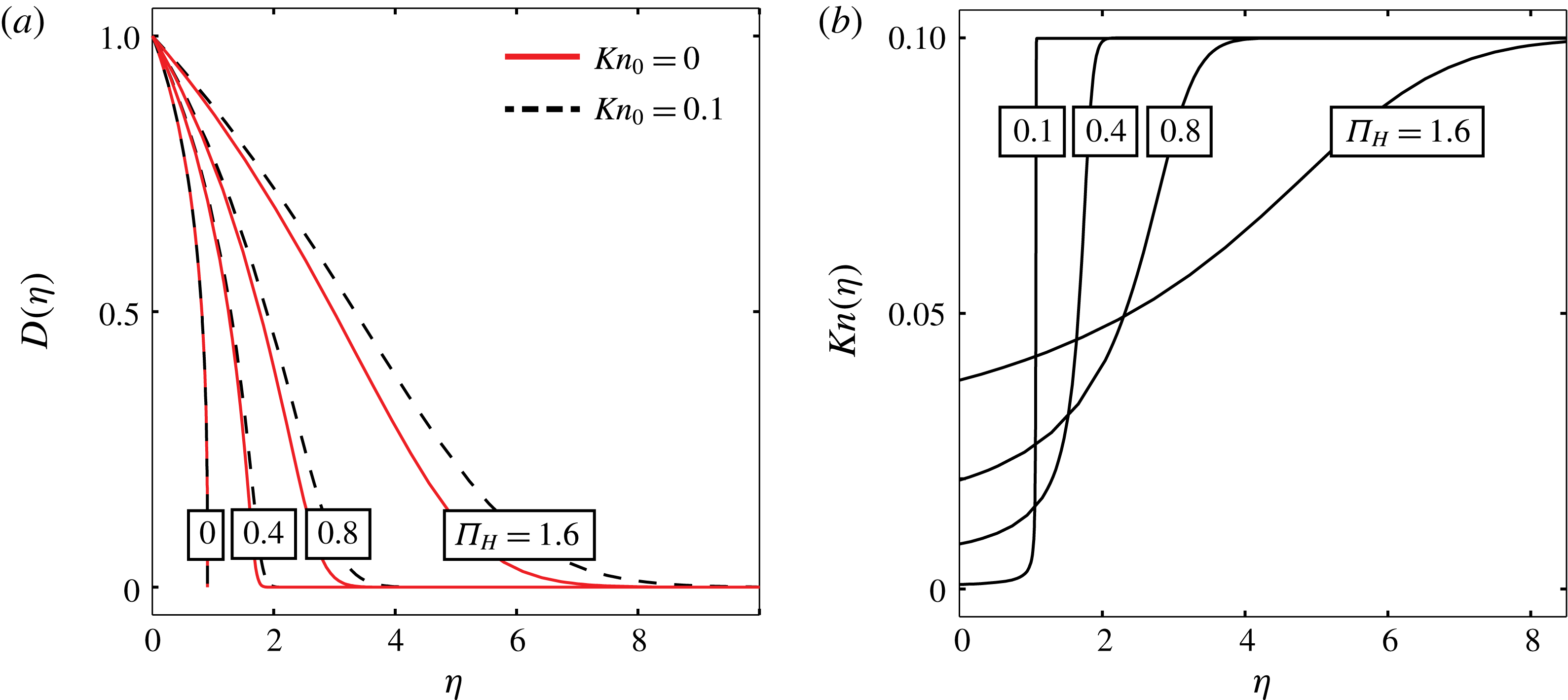
are presented in figure 6(a) for
 $Kn_{0}=0$
(solid lines) and
 $\unicode[STIX]{x1D70E}=1,Kn_{0}=0.1$
(dashed lines). The effect of rarefaction is shown to increase the speed of gas propagation, and reduce the gradients of the deformation. This effect decreases as
 $\unicode[STIX]{x1D6F1}_{H}$
and
 $\unicode[STIX]{x1D6F1}_{P}$
decrease, since
 $Kn_{0}$
is defined ahead of the front, while the local Knudsen number decreases as channel height and pressure increase (see (2.3)). For small
 $\unicode[STIX]{x1D6F1}_{P}$
and
 $\unicode[STIX]{x1D6F1}_{H}$
, the pressure and height in the peeled region are greater compared with the background pressure
 $p_{0}$
and initial channel thickness
 $h_{0}$
. This yields a significantly smaller effective Knudsen number in the peeled region, as illustrated in figure 6(b).
Self-similar solutions with rarefaction effects for
 $\unicode[STIX]{x1D6F1}_{P}=\unicode[STIX]{x1D6F1}_{H}$
and
 $\unicode[STIX]{x1D70E}=1$
. (a) Self-similar deformation profile as a function of the prewetting thickness ratio
 $\unicode[STIX]{x1D6F1}_{H}$
for
 $Kn_{0}=0$
(solid lines) and
 $Kn_{0}=0.1$
(dashed lines). (b) Local Knudsen number as a function of
 $\unicode[STIX]{x1D702}$
for various values of
 $\unicode[STIX]{x1D6F1}_{H}$
for
 $Kn_{0}=0.1$
. Solution based on numerical integration of (4.18).
5 Concluding remarks
The propagation of a gas into micron-sized configurations with linearly elastic boundaries is governed by interaction between effects of low-Mach-number compressibility, rarefaction, elasticity and viscosity. A governing nonlinear evolution equation was derived for the flow field. While exact solutions of this equation are not available, several limiting cases allow solution by self-similarity. These limits correspond to different physical regimes, including: (i) dominant balance between compressibility and viscosity, (PME of order
 $2$
) characterizing compressible flow in rigid microchannels, (ii) dominant balance between elasticity and viscosity, (PME of order
 $4$
) characterizing incompressible flow in elastic microchannels, and (iii) dominant balance involving viscosity, elasticity and compressibility (PME of order
 $2.5$
). Transition of the flow field between the aforementioned regimes and corresponding exact solutions was illustrated for the case of an impulsive mass insertion in which the order of magnitude of the deflection evolves in time. A map of these transitions was presented as a function of the initial channel thickness, the background pressure and stiffness of the spring array. The case where
 $kh_{0}\approx p_{0}$
represents symmetry between compressibility and elasticity, and allowed us to obtain an additional self-similar solution accounting for rarefaction effects.
We note that the analysis presented in §§ 2 and 3 for symmetric displacements about the mid-plane
 $y=0$
can be readily adapted for the case of different stiffness coefficients of the upper and lower substrates (e.g. PDMS channels bonded to glass substrates). In this case we define the total stiffness as
 $k=(p-p_{0})/d=(k_{u}^{-1}+k_{l}^{-1})^{-1}$
(where
 $k_{u}$
and
 $k_{l}$
are the stiffness of the upper and lower surfaces, respectively). For axial flow in the thin annular gap between an elastic shell and an inner rigid cylinder, the stiffness
 $k$
is given by
 $k=Ew_{t}/r_{t}^{2}$
(Elbaz & Gat Reference Elbaz and Gat2016), where
 $E$
is Young’s modulus,
 $w_{t}$
is the shell thickness and
 $r_{t}$
is the radius of the cylinder. In addition, based on Gervais et al. (Reference Gervais, El-Ali, Günther and Jensen2006), for rectangular microchannels
 $k$
can be approximated by
 $k=E/w_{c}c_{1}$
, where
 $w_{c}$
is the width of the channel and
 $c_{1}$
is an order-one proportionality constant. Assuming parabolic deformation, the maximal cross-sectional deflection, taken as
 $d$
, can be linked to the average deflection
 $\langle d\rangle$
by
 $2d/3\sim \langle d\rangle$
. This leads to a minor adjustment in the true mass
 $m$
as a function of the non-dimensional mass
 $M$
,
 $m=(2{p^{\ast }}^{2}lw/3k{\mathcal{R}}\unicode[STIX]{x1D703}_{0})M$
.
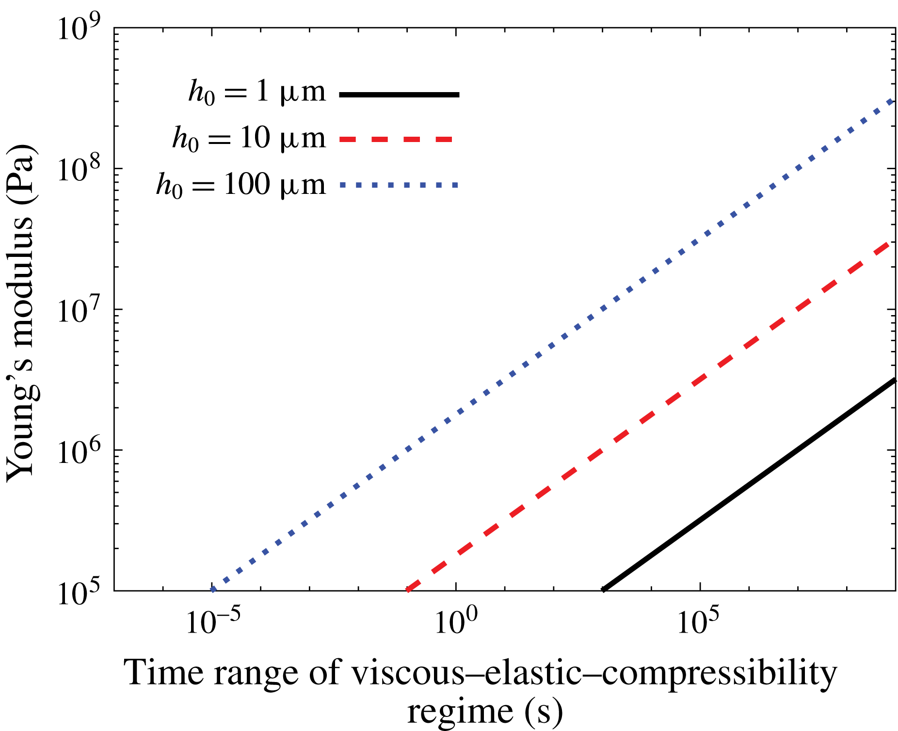
Appendix A presents the dimensional form of the governing evolution equation, the steady-state solution, the early-time compressibility–elasticity–viscosity regime, intermediate-time compressibility–viscosity regime, intermediate-time elasticity–viscosity regime and late-time linearized diffusion regime. While the current work emphasized transitions between the different regimes, in many configurations the propagation dynamics may be limited to a single regime within the time scale of interest. This is illustrated in figure 7, which presents the validity time range of the early compressibility–elasticity–viscosity regime for several initial channel gap values
 $h_{0}$
of
 $1~\unicode[STIX]{x03BC}\text{m}$
(solid black line),
 $10~\unicode[STIX]{x03BC}\text{m}$
(dashed red line) and
 $100~\unicode[STIX]{x03BC}\text{m}$
(dotted blue line). Gas mass
 $m=1~\text{mg}$
of air (viscosity
 $\unicode[STIX]{x1D707}=15\times 10^{-6}~\text{Pa}~\text{s}$
, specific gas constant
 ${\mathcal{R}}=286.9~\text{J}~\text{kg}^{-1}~\text{K}^{-1}$
) is rapidly introduced into a thin gap between two elastic regions with thickness of
 $h_{m}=100h_{0}$
, temperature
 $\unicode[STIX]{x1D703}_{0}=300~\text{K}$
and various values of Young’s modulus (where
 $k=E/h_{m}$
). Very large time scales of the early-time regime characterize
 $h_{0}=1~\unicode[STIX]{x03BC}\text{m}$
channels, or configurations with large values of Young’s modulus
 $E$
, and thus the early-time regime may be valid throughout the time scale of interest.
Time range threshold for the compressibility–elasticity–viscosity early-time regime of impulse-driven air propagation into a shallow elastic microchannel. The time range (s) (horizontal axis) is plotted against substrate Young’s modulus (Pa), for three initial channel heights based on (A 4). The stiffness of the channel was approximated by
 $k=E/h_{m}$
, where
 $h_{m}$
is the thickness of the substrates, taken as
 $h_{m}=100h_{0}$
. Other relevant quantities: viscosity
 $\unicode[STIX]{x1D707}=15\times 10^{-6}~\text{Pa}~\text{s}$
, specific gas constant
 ${\mathcal{R}}=286.9~\text{J}~\text{kg}^{-1}~\text{K}^{-1}$
, temperature
 $\unicode[STIX]{x1D703}_{0}=300~\text{K}$
, mass
 $m=1~\text{mg}$
, channel width
 $w=100~\unicode[STIX]{x03BC}\text{m}$
, background pressure
 $p_{0}=101\,325~\text{Pa}$
.
Appendix A. Results in dimensional form
The governing evolution equation for channel height
 $h$
corresponding to (3.12) reads
 $$\begin{eqnarray}\frac{\unicode[STIX]{x2202}h}{\unicode[STIX]{x2202}t}=\left(\frac{k}{12\unicode[STIX]{x1D707}}\right)\frac{1}{2h-h_{0}+(p_{0}/k)}\frac{\unicode[STIX]{x2202}}{\unicode[STIX]{x2202}x}\left\{\left[h^{3}(h-h_{0}+p_{0}/k)+\frac{6\unicode[STIX]{x1D70E}\unicode[STIX]{x1D706}_{0}p_{0}}{k}h^{2}\right]\frac{\unicode[STIX]{x2202}h}{\unicode[STIX]{x2202}x}\right\},\end{eqnarray}$$
where
 $x$
is the streamwise coordinate,
 $t$
is time,
 $p_{0}$
is the background pressure,
 $\unicode[STIX]{x1D706}_{0}$
is the slip length at atmospheric pressure,
 $h_{0}$
is the undeformed channel height,
 $\unicode[STIX]{x1D70E}$
is the streamwise momentum accommodation coefficient,
 $\unicode[STIX]{x1D707}$
is gas viscosity and
 $k$
is substrate stiffness.
The implicit steady-state solution relating channel streamwise location
 $x$
to gas pressure
 $p$
, corresponding to (4.3), is given by
 $$\begin{eqnarray}\frac{x(p)}{l}=\frac{f(p)-f(p(x=0))}{f(p(x=l))-f(p(x=0))},\end{eqnarray}$$
where
 $$\begin{eqnarray}f(p)=40\unicode[STIX]{x1D70E}\unicode[STIX]{x1D706}_{0}p_{0}k(p-p_{0}+h_{0}k)^{3}+5p(p-p_{0}+h_{0}k)^{4}-(p-p_{0}+h_{0}k)^{5}.\end{eqnarray}$$
The transient early-time (compressibility–elasticity–viscosity regime) solution for the deflection
 $d(x,t)$
in the case of negligible rarefaction effects and corresponding to (4.7) is given by
 $$\begin{eqnarray}d(x,t)=\frac{(60\unicode[STIX]{x1D707})^{1/7}}{k^{5/7}}t^{-1/7}\left[\left(\frac{2{\mathcal{R}}\unicode[STIX]{x1D703}_{0}km}{S_{1}w}\right)^{6/7}-\frac{3(60k^{2}\unicode[STIX]{x1D707})^{4/7}}{35}x^{2}t^{-4/7}\right]_{+}^{1/3},\quad S_{1}=5.0495,\end{eqnarray}$$
where
 $(s)_{_{+}}=\max (s,0)$
,
 $m$
is the initial input mass,
 $w$
the channel width (perpendicular to the
 $(x,y)$
plane),
 ${\mathcal{R}}$
the gas constant and
 $\unicode[STIX]{x1D703}_{0}$
the temperature. The time range for which (A 3) is valid, corresponding to (4.8), is given by
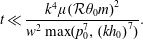 $$\begin{eqnarray}t\ll \frac{k^{4}\unicode[STIX]{x1D707}({\mathcal{R}}\unicode[STIX]{x1D703}_{0}m)^{2}}{w^{2}\max (p_{0}^{7},(kh_{0})^{7})}.\end{eqnarray}$$
The first (compressibility–viscosity branch) intermediate-time solution for the deflection
 $\text{d}(x,t)$
in the case of negligible rarefaction effects and corresponding to (4.10) is given by
 $$\begin{eqnarray}d(x,t)=\frac{(24\unicode[STIX]{x1D707})^{1/3}}{k^{5/3}h_{0}^{4/3}}t^{-1/3}\left[\left(\frac{2{\mathcal{R}}\unicode[STIX]{x1D703}_{0}km}{S_{2}w}\right)^{2/3}-\frac{1}{12}\left(\frac{24k\unicode[STIX]{x1D707}}{h_{0}}\right)^{2/3}x^{2}t^{-2/3}\right]_{+},\quad S_{2}=4.6188.\end{eqnarray}$$
The time range for which (A 5) is valid, corresponding to (4.11), is given by
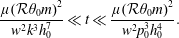 $$\begin{eqnarray}\frac{\unicode[STIX]{x1D707}({\mathcal{R}}\unicode[STIX]{x1D703}_{0}m)^{2}}{w^{2}k^{3}h_{0}^{7}}\ll t\ll \frac{\unicode[STIX]{x1D707}({\mathcal{R}}\unicode[STIX]{x1D703}_{0}m)^{2}}{w^{2}p_{0}^{3}h_{0}^{4}}.\end{eqnarray}$$
The second (elasticity–viscosity branch) intermediate-time solution for the deflection
 $\text{d}(x,t)$
in the case of negligible rarefaction effects and corresponding to (4.13) is given by
 $$\begin{eqnarray}d(x,t)=\frac{(48\unicode[STIX]{x1D707})^{1/5}}{k^{3/5}p_{0}^{2/5}}t^{-1/5}\left[\left(\frac{2{\mathcal{R}}\unicode[STIX]{x1D703}_{0}km}{S_{3}w}\right)^{6/5}-\frac{3p_{0}^{6/5}(48k^{2}\unicode[STIX]{x1D707})^{2/5}}{40}x^{2}t^{-2/5}\right]_{+}^{1/3},\quad S_{3}=6.1441.\end{eqnarray}$$
The time range for which (A 7) is valid, corresponding to (4.14), is given by
 $$\begin{eqnarray}\frac{k^{4}\unicode[STIX]{x1D707}({\mathcal{R}}\unicode[STIX]{x1D703}_{0}m)^{2}}{w^{2}p_{_{0}}^{7}}\ll t\ll \frac{\unicode[STIX]{x1D707}({\mathcal{R}}\unicode[STIX]{x1D703}_{0}m)^{2}}{kw^{2}p_{0}^{2}h_{0}^{5}}.\end{eqnarray}$$
The late-time (linearized regime) solution for the deflection
 $\text{d}(x,t)$
including rarefaction effects and corresponding to (4.16) reads
 $$\begin{eqnarray}\frac{m{\mathcal{R}}\unicode[STIX]{x1D703}_{0}\sqrt{12\unicode[STIX]{x1D707}}}{\sqrt{\unicode[STIX]{x1D70B}kw^{2}p_{0}^{2}h_{0}^{3}(1+h_{0}k/p_{0})(1+6\unicode[STIX]{x1D70E}Kn_{0})t}}\exp \left\{\frac{3(1+h_{0}k/p_{0})\unicode[STIX]{x1D707}x^{2}}{kh_{0}^{3}(1+6\unicode[STIX]{x1D70E}Kn_{0})t}\right\}.\end{eqnarray}$$
The time range for which (A 9) is valid, corresponding to (4.17), is given by
 $$\begin{eqnarray}\frac{\unicode[STIX]{x1D707}({\mathcal{R}}\unicode[STIX]{x1D703}_{0}m)^{2}(1+h_{0}k/p_{0})}{kw^{2}p_{0}^{2}h_{0}^{5}(1+6\unicode[STIX]{x1D70E}Kn_{0})}\ll t.\end{eqnarray}$$
Appendix B. Asymptotic formulation of the assumption of isothermal conditions
In order to assess the order of magnitude of temperature variations for the examined problem we write the dimensional energy equation for a perfect gas (previously omitted from (2.2)),
 $$\begin{eqnarray}\unicode[STIX]{x1D70C}c_{v}\frac{\text{D}\unicode[STIX]{x1D703}}{\text{D}t}=-\unicode[STIX]{x1D735}\boldsymbol{\cdot }\boldsymbol{q}-p\unicode[STIX]{x1D735}\boldsymbol{\cdot }\boldsymbol{u}+\unicode[STIX]{x1D749}\mathbf{: }\unicode[STIX]{x1D735}\boldsymbol{u},\end{eqnarray}$$
where
 $\unicode[STIX]{x1D70C}$
is gas density,
 $c_{v}$
is the specific heat capacity at constant volume,
 $\text{D}$
denotes a material derivative (
 $\text{D}/\text{D}t\equiv \unicode[STIX]{x2202}/\unicode[STIX]{x2202}t+\boldsymbol{u}\boldsymbol{\cdot }\unicode[STIX]{x1D735}$
),
 $\unicode[STIX]{x1D703}$
is gas temperature,
 $t$
is time,
 $\boldsymbol{q}$
is the heat flux density vector satisfying Fourier’s law
 $\boldsymbol{q}=-\unicode[STIX]{x1D705}\unicode[STIX]{x1D735}\unicode[STIX]{x1D703}$
(
 $\unicode[STIX]{x1D705}$
denoting the heat conductivity),
 $p$
is gas pressure,
 $\boldsymbol{u}$
is the gas velocity vector
 $\boldsymbol{u}=(u,v)$
and
 $\unicode[STIX]{x1D749}$
is the Newtonian stress tensor given by (2.2d
). We refer to the previously defined normalized variables in (3.2) and (3.3), and further define the normalized temperature
 $\unicode[STIX]{x1D6E9}=\unicode[STIX]{x1D703}/\unicode[STIX]{x1D703}_{0}$
, the normalized velocity vector
 $\boldsymbol{U}=(U,V)$
, the characteristic streamwise velocity component
 $u^{\ast }$
(where
 $u=u^{\ast }U$
), the characteristic density
 $\unicode[STIX]{x1D70C}^{\ast }$
(where
 $\unicode[STIX]{x1D70C}=\unicode[STIX]{x1D70C}^{\ast }\unicode[STIX]{x1D6EC}$
), the kinematic viscosity
 $\unicode[STIX]{x1D708}^{\ast }=\unicode[STIX]{x1D707}/\unicode[STIX]{x1D70C}^{\ast }$
, the thermal diffusivity
 $\unicode[STIX]{x1D6FC}$
and the heat capacity ratio
 $\unicode[STIX]{x1D6FE}_{c}$
. Normalizing (B 1) according to these definitions we may derive the leading-order energy equation in non-dimensional form,
 $$\begin{eqnarray}\displaystyle \frac{\unicode[STIX]{x1D700}^{2}}{\unicode[STIX]{x1D6FE}_{c}}\left(\frac{\unicode[STIX]{x1D708}^{\ast }}{\unicode[STIX]{x1D6FC}}\right)\left(\frac{u^{\ast }l}{\unicode[STIX]{x1D708}^{\ast }}\right)\unicode[STIX]{x1D6EC}\frac{\text{D}\unicode[STIX]{x1D6E9}}{\text{D}T} & = & \displaystyle \left[\frac{\unicode[STIX]{x2202}^{2}\unicode[STIX]{x1D6E9}}{\unicode[STIX]{x2202}Y^{2}}+O(\unicode[STIX]{x1D700}^{2})\right]-\unicode[STIX]{x1D700}^{2}\frac{\unicode[STIX]{x1D6FE}_{c}-1}{\unicode[STIX]{x1D6FE}_{c}}\left(\frac{\unicode[STIX]{x1D708}^{\ast }}{\unicode[STIX]{x1D6FC}}\right)\left(\frac{u^{\ast }l}{\unicode[STIX]{x1D708}^{\ast }}\right)P\unicode[STIX]{x1D735}_{N}\boldsymbol{\cdot }\boldsymbol{U}\nonumber\\ \displaystyle & & \displaystyle +\,(\unicode[STIX]{x1D6FE}_{c}-1)\left(\frac{\unicode[STIX]{x1D708}^{\ast }}{\unicode[STIX]{x1D6FC}}\right)\frac{{u^{\ast }}^{2}}{\unicode[STIX]{x1D6FE}_{c}{\mathcal{R}}\unicode[STIX]{x1D703}_{0}}\left[\left(\frac{\unicode[STIX]{x2202}U}{\unicode[STIX]{x2202}Y}\right)^{2}+O(\unicode[STIX]{x1D700}^{2})\right],\end{eqnarray}$$
where
 $\text{D}/\text{D}T\equiv \unicode[STIX]{x2202}/\unicode[STIX]{x2202}T+\boldsymbol{U}\boldsymbol{\cdot }\unicode[STIX]{x1D735}_{N}$
and
 $\unicode[STIX]{x1D735}_{N}$
is the equivalent non-dimensional operator. Noting the definitions of the Reynolds number
 $Re=u^{\ast }l/\unicode[STIX]{x1D708}^{\ast }$
(see also (3.5a,b
)), the Prandtl number
 $Pr=\unicode[STIX]{x1D708}^{\ast }/\unicode[STIX]{x1D6FC}$
and the Mach number
 $Ma=u^{\ast }/\sqrt{\unicode[STIX]{x1D6FE}_{c}{\mathcal{R}}\unicode[STIX]{x1D703}_{0}}$
, the order of magnitude of temperature variations may be written
 $$\begin{eqnarray}\unicode[STIX]{x0394}\unicode[STIX]{x1D6E9}=O(\unicode[STIX]{x1D700}^{2}Pr\,Re,Pr\,Ma^{2}).\end{eqnarray}$$
Since the Prandtl number for common gases (e.g. air, nitrogen etc.) is
 $Pr\approx 0.7{-}0.8$
, isothermal flow is achieved for sufficiently small
 $\unicode[STIX]{x1D700}^{2}Re,Ma^{2}\ll 1$
, assuming the boundaries of the configuration are maintained at constant temperature. These values correlate to experimental results of rigid-walled gaseous microflows (e.g. Arkilic et al.
Reference Arkilic, Schmidt and Breuer1997; Zohar et al.
Reference Zohar, Lee, Lee, Jiang and Tong2002).



