


I. INTRODUCTION
Wireless power transfer technology has been developing quickly and found many applications in areas such as moist harsh environments, charging the batteries of electric vehicles [Reference Covic, Boys, Tam and Peng1, Reference James, Boys and Covic2], portable electronic devices [Reference Si, Hu, Malpas and Budgett3, Reference Hsu and Hu4], and implanted electronic devices [Reference Si, Hu, Malpas and Budgett5, Reference Hamill and Bina6], etc. Among a number of choices to transfer power wirelessly, inductive power transfer (IPT) is the most developed one so far. As there is usually a relatively large gap between the primary and secondary coils of an IPT system, its power transfer ability and efficiency are greatly limited compared with traditional tightly-coupled transformers and electric motors. To solve this problem, three major techniques are usually adopted, i.e. increasing the frequency of the system, improving the coupling degree between the primary and secondary coils, and taking advantage of the principles of resonance.
To maintain resonant operation for an IPT system and realize soft-switching, one method is to adjust the zero voltage switching (ZVS) frequency of the system dynamically to match the gate driving frequency. Traditionally, this is realized through switching mode capacitors [Reference Al-Kuran7–Reference Perez-Nicoli, Castro and Silveira13] or inductors [Reference Aghdam, Babaei and Zadeh14–Reference Tang, Fu, Wang and Xu22]. However, there are a few disadvantages with the conventional methods, such as complexity in circuit structure and control strategy, high electro magnetic interference (EMI), the frequency not being able to be adjusted smoothly, etc. A Balanced-voltage-controlled Variable Capacitor Structure has been proposed in the conference paper [Reference Tian and Hu23], but more detailed theoretical analysis and experimental results are necessary.
This paper proposes a Voltage-controlled Variable Capacitor Structure (VVCS) to adjust the ZVS frequency of an autonomous push–pull converter though a DC voltage. The DC voltage controls the conduction period of a diode in the VVCS. The equivalent capacitance of the VVCS changes with the variation of the conduction period of the diode. The basic operating principle of the method is explained in Section II of this paper. Section III presents theoretical modeling of the circuit. The experimental results are provided in Section IV. Finally Section V draws the conclusions.
II. THE PROPOSED METHOD AND BASIC OPERATING PRINCIPLE
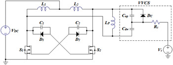
Figure 1 shows the proposed VVCS applied to the resonant tank of an autonomous push–pull converter that has been introduced in section 7.3 of [Reference Hu24]. As can be seen, the common fixed value resonant capacitor in the resonant tank of the autonomous push–pull converter is replaced by the VVCS as shown in the dashed block consisting of C up , Cdw, Dc , and R c . The equivalent capacitance C e of the VVCS can be changed by the control voltage V c . The higher V c is, the larger the equivalent capacitance C e , and the lower the ZVS frequency f zvs of the converter.
The proposed VVCS applied to the autonomous push–pull converter.

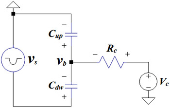
The reason that the equivalent capacitance C e can be controlled by the voltage V c is that V c influences the conduction period T con of the diode D c . The higher V c is, the longer T con is, because the higher V c is, the larger the voltage on the anode of the diode D c . When the diode conducts, C up is shorted so that the equivalent capacitance of the VVCS is C dw , while when the diode is off, the equivalent capacitance of the VVCS is C up and C dw in series. As the capacitance of C dw is larger than that of C up and C dw in series, the longer the diode conducts, the larger the equivalent capacitance of the VVCS is.
III. THEORETICAL MODELING
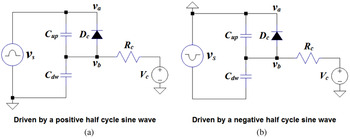
The goal of the theoretical analysis is to find the relationship between the equivalent capacitance C e of the VVCS and the control voltage V c . For this purpose, the circuit in Fig. 1 is simplified as the ones shown in Fig. 2, which include only C up , Cdw, Dc, Rc , and V c of the original circuit and is driven periodically with positive and negative half cycle sinusoidal waves v s in turn as being the same case as in the original circuit.
The simplified circuit for theoretical analysis of the VVCS.

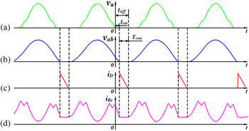
Figure 3 shows the typical waveforms of v
a
, vab
, the current i
D
and
 $i_{R_c}$
flowing through the diode D
c
, and the resistor R
c
, respectively, in steady state. The period when i
D
is not zero represents the conduction period T
con
of the diode D
c
. It can be seen from Fig. 3 that the diode turns on when the voltage across it (v
ab
) is zero and turns off when both the voltage across it (v
ab
) and the current flowing through it (i
D
) drops to zero. So the switching condition of the passive diode is very good, which helps to keep EMI low. This is achieved at the expense of higher power loss at the control resistor R
c
. As can be seen from Fig. 3(d), a continuous current
 $i_{R_c}$
flows through the resistor R
c
. The value of
 $i_{R_c}$
depends upon the values of R
c
and the control voltage V
c
. Smaller R
c
and larger V
c
lead to higher
 $i_{R_c}$
. So within the control range, larger R
c
and smaller V
c
are preferred.
Typical wave forms of the circuit: v
a
, vab, iD
, and
 $i_{R_{\rm c}} $
.

The major task of the theoretical analysis part is to derive the relationship between C e and V c , which is carried out in three steps. Firstly, the relationship between T con and V c is derived. Secondly, the relationship between C e and T con is found out. Finally, the relationship between C e and V c is calculated based on the above two relationships. To find out the relationship between T con and V c , two exact moments, i.e. the moment the diode starts to conduct- “t on ” and the moment the diode stops to conduct- “t off ” need to be determined first. After that, T con can be calculated with (1):
 $$T_{con} = t_{off} - t_{on}. $$
A. Determination of the moment the diode stops to conduct
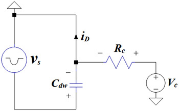
Figure 4 shows the equivalent circuit of Fig. 2(b) when the diode is conducting. C up and D c are removed because an ideal conducting diode amounts to a short-circuit.
The equivalent circuit when the diode is conducting.

The diode is regarded as stopping to conduct when the current flowing through it (i D ) drops to zero, where i D is governed by (2):
 $$i_D = C_{dw} \displaystyle{{{\rm d}v_s} \over {{\rm d}t}} + \displaystyle{{V_c} \over {R_c}}. $$
Substitute v s = A s sinωt and i D = 0 into (2), the moment the diode stops to conduct t off can be derived as:
 $$t_{off} = \displaystyle{{{\rm arccos}\left( { - \displaystyle{{V_c} \over {\omega A_s R_c C_{dw}}}} \right)} \over \omega}, $$
where A s is the magnitude of the voltage of the resonant tank of the autonomous push–pull converter, which is roughly π times the voltage of the DC voltage source V DC [Reference Hu24, Reference Si, Hu, Budgett, Malpas, Yang and Gao25].
According to simulation and the theoretical analysis result as shown in (3), the value of ωt off varies between π/2 and π when the value of V c varies between 0 and ωA s RcCdw .
B. Determination of the moment the diode starts to conduct
Figure 5 shows the equivalent circuit when the diode is not conducting, regarded as open so as to be removed from the circuit.
The equivalent circuit when the diode is not conducting.

The voltage at the anode of the diode v b is governed by (4):
 $$\displaystyle{{{\rm d}v_b} \over {{\rm d}t}} + \displaystyle{1 \over {R_c (C_{up} + C_{dw} )}} \cdot v_b = \displaystyle{{\omega A_s R_c C_{dw} {\rm cos}\omega t + V_c} \over {R_c (C_{up} + C_{dw} )}}.$$
The solution of (4) is:
 $$v_b = \omega k_1 {\rm sin}\omega t + kk_1 {\rm cos}\omega t + V_c + Ke^{ - kt}, $$
Where
 $$k = \displaystyle{1 \over {R_c(C_{up} + C_{dw})}}{\rm }\comma \;k_1 = \displaystyle{{\omega A_sC_{dw}} \over {(C_{up} + C_{dw})(\omega ^2 + k^2)}}.$$
The constant K in (5) can be determined by the initial condition, i.e. the value of v b at the moment of t 2 (refer to Fig. 3). The moment t 2 can be expressed by (6):
 $$t_2 = t_{off} - \displaystyle{{2\pi} \over \omega}. $$
Substitute (3), (6) and v b = 0 into (5), the constant K can be derived as:
 $$K = \displaystyle{{ - \omega k_1 \sqrt {1 - k_2 ^2} + kk_1 k_2 - V_c} \over {e^{ - k \cdot \displaystyle{{{\rm arccos}( - k_2 ) - 2\pi} \over \omega}}}}, $$
where
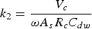 $k_2 = \displaystyle{{V_c} \over {\omega A_s R_c C_{dw}}}$
.
It can be seen from Fig. 3 that the diode starts to conduct when v b becomes zero. Substituting v b = 0 into (5) gives:
 $$\omega k_1 \cdot {\rm sin}\omega t + kk_1 \cdot {\rm cos}\omega t + V_c + Ke^{ - kt} = 0.$$
The exponential component Ke −kt in (8) relates to the transient response of the circuit, which does not change much during a short time period of one or half a cycle of v b , which is usually much smaller than the time constant τ of the circuit determined by the product of the capacitor and resistor R c (C up + C dw ). Consequently, Ke −kt can be set roughly at a constant value Ke −kt c , where t c can be simply zero. However, the closer t c is to the moment the diode starts to conduct t on , the smaller the error it causes.
From (8), the moment the diode starts to conduct can be derived as (9):
 $$t_{on} \approx \displaystyle{{{\rm arcsin}\left( { - \displaystyle{{V_c + Ke^{ - kt_c}} \over {k_1 \sqrt {\omega ^2 + k^2}}}} \right) - {\rm arctan}\displaystyle{k \over \omega}} \over \omega}. $$
The value of ωt on varies between 0 and π/2, which is in consistent with what has been observed from a wide range of simulation studies.
C. The relationship between T con and V c
Substitute (3) and (9) into (1), the conduction period T con of the diode can be derived as:
 $$\eqalign{T_{con} \approx &\eqalign{&\displaystyle{{{\rm arccos}\left( { - \displaystyle{{V_c} \over {\omega A_s R_c C_{dw}}}} \right) + {\rm arcsin}\left( {\displaystyle{{V_c + Ke^{ - kt_c}} \over {k_1 \sqrt {\omega ^2 + k^2}}}} \right) }}\cr &+ {\rm arctan}\displaystyle{k \over \omega}} \over \omega}. $$
When the circuit quality factor Q is high, the angular frequency ω in (10) can be simplified as the undamped natural oscillation frequency as expressed by (11):
 $$\omega = 2\pi f = \displaystyle{1 \over {\sqrt {LC}}}. $$
Substitute (11) into (10) gives (12),
 $$\eqalign{T_{con} &= \sqrt {LC_{on}} \cdot \left( {{\rm arccos}\left( { - \displaystyle{{V_c \cdot \sqrt {LC_{on}}} \over {A_s R_c C_{dw}}}} \right) }\right.\cr & \left. \quad- {\rm arcsin}\left( { - \displaystyle{{V_c + Ke^{ - kt_c}} \over {k_1 \sqrt {\displaystyle{1 \over {LC_{off}}} + k^2}}}} \right.) + {\rm arctan}(k\sqrt {LC_{off}} ) \right)}$$
where C on and C off represent the capacitance of the circuit when the diode is on and off, respectively, as expressed by (13) and (14):
 $$C_{on} = C_{dw} \comma$$
 $$ C_{off} = \displaystyle{{C_{up} C_{dw}} \over {C_{up} + C_{dw}}}. $$
D. The relationship between C e and V c
To find the relationship between C e and V c , the relationship between C e and T con needs to be found first, which can then be combined with (12) to get the relationship between C e and V c . Derivation of the relationship between C e and T con is based on a LC parallel resonance circuit. The frequency of such a circuit is governed by (11). From (11), the equivalent capacitance of the circuit can be derived as:
 $$C_e = \displaystyle{1 \over {L \cdot (2\pi f)^2}} = \displaystyle{{T^2} \over {4\pi ^2 L}}\comma$$
where T represents the period of one cycle, i.e. the reciprocal of the frequency “f”. Suppose that the inductance of the parallel LC resonance circuit is fixed while the capacitance of the parallel LC resonance circuit switches between two distinct values C on and C off periodically and their duration are t on and t off , respectively. According to (15), the equivalent capacitance C e of the circuit is:
 $$C_e = \displaystyle{{(t_{on} + t_{off} )^2} \over {4\pi ^2 L}}.$$
Actually t on equals T con , and t off can be derived based on the principle that the wave forms when the capacitance is C on and C off , respectively, need to go continuously into each other. Finally the relationship between C e and T con is derived as (17):
 $$C_e = \displaystyle{{\left( {2\pi \sqrt {LC_{off}} + \left( {1 - \sqrt {\displaystyle{{C_{off}} \over {C_{on}}}}} \right) \cdot T_{con}} \right)^2} \over {4\pi ^2 L}}.$$
Substituting (12) into (17) gives the relationship between C e and V c as expressed by (18):
 $$\eqalign{C_e & = \left[ \sqrt {C_{off}} + \displaystyle{{\sqrt {C_{on}} - \sqrt {C_{off}}} \over {2\pi}} \left({\rm arccos}\left( - \displaystyle{{V_{\rm c} \sqrt {LC_{{\rm on}}}} \over {A_{\rm s} R_{\rm c} C_{{\rm dw}}}}\right)\right.\right. \cr & \quad \left. \left. - \arcsin \left({ - \displaystyle{{V_c + Ke^{ - kt_c}} \over {k_1 \sqrt {\displaystyle{1 \over {LC_{off}}} + k^2}}}}\right) + {\rm arctan}(k\sqrt {LC_{off}})\right) \right]^{2}}.$$
Equation (18) can be simplified as (19):
 $$C_e = \left[ {\sqrt {C_{off}} + \displaystyle{{\sqrt {C_{on}} - \sqrt {C_{off}}} \over {2\pi}} \cdot T_{rad}} \right]^{2}\comma $$
where:
 $$T_{rad} = {\rm arccos}\left( { - \displaystyle{{V_c \sqrt {LC_{on}}} \over {A_s R_c C_{dw}}}} \right) - \arcsin \left( { - \displaystyle{{V_c + Ke^{ - kt_c}} \over {k_1 \sqrt {\displaystyle{1 \over {LC_{off}}} + k^2}}}} \right) + {\rm arctan}(k\sqrt {LC_{off}} ).$$
Actually, T rad is the diode conduction period T con in radians. Theoretically, T rad changes from 0 to 2π. When T rad is 0, (19) becomes:
 $$C_e = C_{off}. $$
It means that when the diode conduction period is 0, the equivalent capacitance is C off , which coincides exactly with the real circuit situation. While when T rad is 2π (meaning that the diode always conducts so as to be equivalent to a short-circuit), (19) becomes:
 $$C_e = C_{on}. $$
Again, this is in agreement with the basic concept and practical circuit situation.
It can be seen from (21) and (22) that theoretically the equivalent capacitance of the VVCS changes between C on and C off , which correspond to C dw and the capacitance of C up and C dw in series, respectively, as can be seen from (13) and (14). So the variation range of the equivalent capacitance of the VVCS is determined by the values of the two capacitors C up and C dw . When the value of C dw is fixed, a smaller C up results in a larger the variation range of the VVCS. When the values of C up and C dw are fixed, a smaller value of R c leads to larger adjustable range of the VVCS with the same variation range of the control voltage V c .
E. The relationship between f zvs and V c
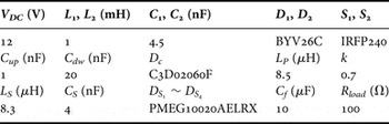
Substituting (18) into (11) gives the relationship between f zvs and V c as expressed by (23). Figure 8 in Section IV shows the theoretical relationship between the ZVS frequency f zvs and the control voltage V c got from (23) using parameters as shown in Table 1 of Section IV together with the experimental results, from which it can be seen that the theoretical and experimental results agree with each other quite well.
 $$f_{zvs} = \displaystyle{{1} \over {\eqalign{ & 2\pi \sqrt L \cdot \left( \sqrt {C_{off}} + \displaystyle{{\sqrt {C_{on}} - \sqrt {C_{off}}} \over {2\pi}} \left( {\rm arccos}\left({ - \displaystyle{{V_{\rm c} \sqrt {LC_{{\rm on}}}} \over {A_{\rm s} R_{\rm c} C_{{\rm dw}}}}} \right)\right. \right. \cr & \left. \left. - \arcsin \left({ - \displaystyle{{V_c + Ke^{ - kt_c} \over {k_1 \sqrt {\displaystyle{1 \over {LC_{off}}} + k^2}}}}}\right) + {\rm arctan}(k\sqrt {LC_{off}})\right)\right)}}}.$$
IV. EXPERIMENTAL RESULTS
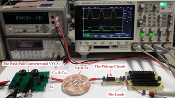
Figure 6 shows the experimental setup, which includes the push–pull converter and the VVCS (refer to Fig. 1), the primary and secondary side coils L
P
and L
S
, and the parallel tuning, full-bridge regulation pick-up circuit. Table 1 shows the components and parameters of the primary and secondary side circuits, where C
s
is the parallel tuning capacitor of the pick-up circuit,
 $D_{{\rm s}_{\rm 1}} \sim D_{{\rm s}_{\rm 4}}$
the regulation diodes, C
f
the filter capacitor, and R
load
the load resistance.
The experimental setup.

Parameters and components of the primary and secondary side circuits.

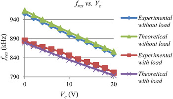
Figure 7 shows the experimental and theoretical relationships between the operating frequency of the converter and the control voltage V c together under two different situations, i.e. when there is (R load = 100 Ω) and there is no load, from which it can be seen that the theoretical and experimental results agree with each other quite well. It shows that the operating frequency is negatively related to the control voltage V c because the higher V c is, the larger the equivalent capacitance of the VVCS as explained in Sections II and III.
Experimental and theoretical relationships between the frequency of the converter and the control voltage.

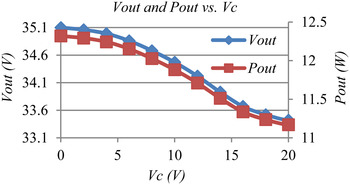
Figure 8 shows the experimental relationships of the output voltage V out and power P out against the control voltage V c when the load resistance R load is 100 Ω. As the circuit is designed to resonant when the control voltage is zero, the output voltage decreases with the increase of the control voltage because the higher the control voltage is, the larger the equivalent capacitance of the VVCS and therefore the lower the frequency of the converter becomes, so that the operating frequency deviates from the resonant frequency further.
Experimental relationships of the output voltage V out and power P out against the control voltage V c .

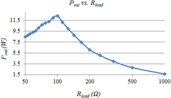
Figure. 9 shows the relationship between the load resistance R load and the output power P out when the control voltage V c is zero, from which it can be seen that the output power changes with the change of the load resistance, and reaches the maximum power of about 12 W when the load resistance is 100 Ω.
Experimental relationship between the output power P out and the load resistance R load .

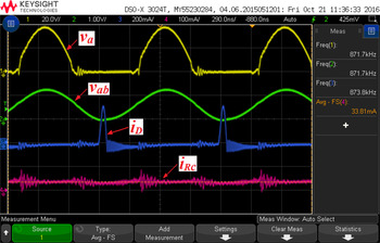
Figure 10 shows the experimental waveforms of v
a
, vab
, the current i
D
, and
 $i_{R_{\rm c}}$
flowing through the diode D
c
and the resistor R
c
, respectively, from which it can be seen that a short period transition from on to off of the diode D
c
causes negligible distortion in its voltage (v
ab
) because of the favorable switching conditions of the diode.
Experimental waveforms of v
a
, vab
and the current i
D
and
 $i_{R_{\rm c}} $
flowing through D
c
and R
c
.

V. CONCLUSIONS
This paper proposes a new method to adjust the ZVS frequency of an autonomous push–pull converter by replacing the common fixed value resonant capacitor in the resonant tank with a VVCS. The equivalent capacitance of the VVCS can be adjusted simply with a DC voltage, which influences the ZVS frequency, and therefore the output voltage and power of the IPT system. As a passive diode instead of an active switch is used to control the conduction time of a capacitor in the VVCS, the equivalent capacitance of the VVCS can be adjusted more smoothly with less EMI than traditional switch mode capacitors. Mathematical models for the relationship between the equivalent capacitance of the VVCS and the frequency of the converter against the control voltage is developed, and practical experiments are carried out to prove their validity.
 Jianlong Tian received his B.S. degree in Mechanical and Electric Engineering from the Agricultural University of Hebei, Baoding, China, in 1989; and his M.S. degree in Detection Technology and Automatic Equipment from the Beijing University of Chemical Technology, Beijing, China, in 2003. He has been working towards his Ph.D. degree at the University of Auckland, Auckland, New Zealand, since 2012. For more than eight years he worked as an Electronic Engineer for a couple of companies in Beijing, China. His current research interest include the high frequency and resonant operation of IPT systems, voltage controlled variable capacitors and soft-switching DC-AC power converters.
 Dr. Aiguo Patrick Hu received his B.S. and M.S. degrees from Xian Jiaotong University, Xian, China, in 1985 and 1988, respectively; and his Ph.D. degree from the University of Auckland, Auckland, New Zealand, in 2001. He served as a Lecturer and as a Director of the China Italy Cooperative Technical Training Center in Xian, China, and as the General Manager of a technical development company. He stayed for a semester at the National University of Singapore (NUS), Singapore, as an Exchange Postdoctoral Research Fellow with funding from the Asian2000 Foundation. Patrick is a leading researcher in the field of wireless power technologies. He holds 15 patents in wireless/contactless power transfer and microcomputer control technologies, has published papers in more than 200 peer reviewed journal and conference proceedings and has over 2600 citations. He authored the first monograph on wireless inductive power transfer technology, and contributed 4 book chapters on inductive power transfer modeling/control as well as electrical machines. Patrick is currently with the Department of Electrical and Electronic Engineering, University of Auckland, Auckland, New Zealand. He is also the Head of Research of PowerbyProxi Ltd, as well as a Guest Professor of Chongqing University, Chongqing, China, and Taiyuan University of Technology, Taiyuan, China. He is a Senior Member of IEEE, a former Chairman of IEEE NZ Power Systems/Power Electronics Chapter, and the current Chairman of the NZ North Section. He served as Secretary/Treasurer of the NZ Chinese Scientists Association, and is now the Vice President. His current research interests include wireless/contactless power transfer systems, and the application of power electronics in renewable energy systems.