1 Introduction
A conglomeration of discrete macroscopic particles characterized by dissipative collisions is termed as a granular material. Granular materials are prevalent in various industries – for instance in the chemical, agriculture and food industries – as well as in nature – for instance in the asteroid belt, sand dunes, debris, etc. Under substantially strong driving forces (e.g. vibration, shearing, etc.), granular materials are in the rapid flow regime, in which they exhibit fluid-like behaviour and are often referred to as granular gases (Campbell Reference Campbell1990; Goldhirsch Reference Goldhirsch2003). In the rapid flow regime, the particles of a granular material move randomly and, similarly to a monatomic gas, it can be assumed that the collisions among them are binary and instantaneous. However, in contrast to a monatomic gas, the collisions between any two particles of a granular material are inherently inelastic, and thereby energy is dissipated during each collision. The inelastic collisions in granular materials lead to many interesting phenomena – for instance standing wave patterns (Melo, Umbanhowar & Swinney Reference Melo, Umbanhowar and Swinney1995; Umbanhowar, Melo & Swinney Reference Umbanhowar, Melo and Swinney1996), clustering (Kudrolli, Wolpert & Gollub Reference Kudrolli, Wolpert and Gollub1997), fingering (Pouliquen, Delour & Savage Reference Pouliquen, Delour and Savage1997), mixing and segregation (Mullin Reference Mullin2000; Ottino & Khakhar Reference Ottino and Khakhar2000; Breu et al. Reference Breu, Ensner, Kruelle and Rehberg2003), shear banding (Mueth et al. Reference Mueth, Debregeas, Karczmar, Eng, Nagel and Jaeger2000; Shukla & Alam Reference Shukla and Alam2009), jamming (Corwin, Jaeger & Nagel Reference Corwin, Jaeger and Nagel2005), density waves (Liss, Conway & Glasser Reference Liss, Conway and Glasser2002; Alam, Chikkadi & Gupta Reference Alam, Chikkadi and Gupta2009), etc. Nevertheless, the mechanics of granular material is still not well-understood, although there have been significant developments in the last couple of decades.
The analogy between granular and molecular fluids has motivated several researchers to devise theoretical methods for studying granular fluids based on the kinetic theory within the framework of the Boltzmann equation; see, e.g., Jenkins & Richman (Reference Jenkins and Richman1985a
,Reference Jenkins and Richman
b
), Goldshtein & Shapiro (Reference Goldshtein and Shapiro1995), Brey, Moreno & Dufty (Reference Brey, Moreno and Dufty1996), Brey et al. (Reference Brey, Dufty, Kim and Santos1998a
), Sela & Goldhirsch (Reference Sela and Goldhirsch1998), Garzó & Santos (Reference Garzó and Santos2003), Bisi, Spiga & Toscani (Reference Bisi, Spiga and Toscani2004), Brilliantov & Pöschel (Reference Brilliantov and Pöschel2004) and Kremer, Santos & Garzó (Reference Kremer, Santos and Garzó2014). Kinetic theory for granular flows was first introduced in the two seminal papers by Jenkins & Savage (Reference Jenkins and Savage1983) and Lun et al. (Reference Lun, Savage, Jeffrey and Chepurniy1984), the former of which deals with the theory for nearly elastic granular flows while the latter with arbitrary inelasticity. The reported works on the kinetic theory for granular fluids also attempted to extend the two well-known approximation methods in the kinetic theory for monatomic gases, namely the Chapman–Enskog (CE) expansion (Chapman & Cowling Reference Chapman and Cowling1970) and Grad’s method of moments (Grad Reference Grad1949b
). Despite the fact that the higher-order approximations (Burnett and beyond) resulting from the CE expansion lead to unstable equations while Grad’s method of moments always yields linearly stable sets of equations in the case of monatomic gases (Bobylev Reference Bobylev1982), the former has been studied extensively even for granular gases. Goldshtein & Shapiro (Reference Goldshtein and Shapiro1995) applied the CE expansion to obtain Euler-like hydrodynamic equations for rough granular flows. The papers by Brey et al. (Reference Brey, Dufty, Kim and Santos1998a
) and Garzó & Dufty (Reference Garzó and Dufty1999) applied the CE expansion to dilute and dense granular gases respectively to derive the first-order (Navier–Stokes and Fourier) constitutive relations for the system of mass, momentum and energy balance equations. Both the works assumed that the space and time dependence of the distribution function can be expressed completely in terms of the hydrodynamic fields and represented the distribution function in a formal series of a uniformity parameter that measures the strength of the spatial gradients of the hydrodynamic fields. Sela, Goldhirsch & Noskowicz (Reference Sela, Goldhirsch and Noskowicz1996) performed a generalized expansion on the distribution function in powers of two small parameters, namely the Knudsen number and the degree of inelasticity
 $\unicode[STIX]{x1D716}=1-e^{2}$
, where
 $e$
is the coefficient of (normal) restitution, and determined the constitutive relations up to Burnett order for the system of mass, momentum and energy balance equations specialized to a simply sheared two-dimensional hard-sphere granular gas via the CE expansion. Subsequently, with the same method, Sela & Goldhirsch (Reference Sela and Goldhirsch1998) (see also Gupta Reference Gupta2011) determined the constitutive relations up to Burnett order for a smooth hard-sphere granular gas in three dimensions. However, both of these works restricted the coefficient of restitution to very close to
 $1$
in order to get the zeroth-order solution in the expansion as Maxwellian, similarly to a monatomic gas. Lutsko (Reference Lutsko2005) employed the CE expansion to obtain the constitutive relations for dense granular gases with arbitrary energy loss models. His model produced the homogeneous cooling state (HCS) solution at the zeroth order in the expansion while Navier–Stokes and Fourier constitutive relations at first order. Following the approach of expanding the distribution function in powers of the uniformity parameter, Khalil, Garzó & Santos (Reference Khalil, Garzó and Santos2014) recently obtained the Burnett-order constitutive relations for a smooth granular gas described with (inelastic) Maxwell interaction potential via the CE expansion. It is worth pointing out that, unlike Sela & Goldhirsch (Reference Sela and Goldhirsch1998), their approach did not restrict the coefficient of restitution to close to
 $1$
. Recently, Kremer et al. (Reference Kremer, Santos and Garzó2014) employed the CE expansion to obtain the transport coefficients up to Navier–Stokes order for a granular gas of rough hard spheres.
Despite the success of Grad’s method of moments over the CE expansion in the case of monatomic gases (see, e.g., Torrilhon Reference Torrilhon2016, and references therein), the former in the case of granular flows has received much less attention than the latter which has been investigated extensively. Nevertheless, over the last few years, researchers have shown interest in exploring the former method as well (see, e.g., Kremer & Marques Jr Reference Kremer and Marques2011; Garzó Reference Garzó2013; Saha & Alam Reference Saha and Alam2014). The pioneering work on Grad’s method of moments for granular flows is due to Jenkins & Richman, who extended the method to granular flows and derived the Grad 13-moment (G13) equations for a dense and smooth granular gas in Jenkins & Richman (Reference Jenkins and Richman1985a
) and, subsequently, the Grad 16-moment equations for a dense and rough two-dimensional granular gas in Jenkins & Richman (Reference Jenkins and Richman1985b
) – the extra field variables in the latter work are due to rotational motion of rough particles on collision. Bisi et al. (Reference Bisi, Spiga and Toscani2004) further extended Grad’s method of moments to weakly inelastic granular flows with variable coefficient of restitution, although in one dimension. As it is well established that the scalar fourth moment is necessary for the proper description of a granular gas, Risso & Cordero (Reference Risso and Cordero2002) included the scalar fourth moment and – for a granular gas – obtained the Grad moment equations for nine hydrodynamic fields in two dimensions (corresponding to
 $14$
field variables in three dimensions), and applied them to investigate two problems, namely the HCS and a granular system steadily heated by two parallel walls. Kremer & Marques Jr (Reference Kremer and Marques2011) presented the Grad 14-moment (G14) theory for dilute granular gases, and by employing this theory they investigated the HCS, found the constitutive relations for five-moment equations and performed eigenmode analysis on 13-field theory, where they assumed a constant value for the scalar fourth moment. Garzó (Reference Garzó2013) demonstrated the G14 theory for moderately dense granular flows, although the work aimed at finding the Navier–Stokes level constitutive relations through the G14 equations. Recently, Saha & Alam (Reference Saha and Alam2014) developed Grad’s method of moments based on an anisotropic Gaussian and employed it to investigate the non-Newtonian stress, collisional dissipation and heat flux in a sheared two-dimensional granular flow.
The main reasons, among others, why Grad’s method of moments for granular flows is receiving less attention could be that (i) the production terms, which emanate through the Boltzmann collision integral, in the moment equations are very difficult to evaluate for a general interaction potential, (ii) how many and which moments one should consider for describing a process is not known a priori and (iii) the boundary conditions associated with the Grad moment equations are unclear, which is apparently also the case for higher-order equations resulting from the CE expansion. Over the last couple of years, two of the present authors have developed a computational methodology that can compute the production terms associated with the Grad moment equations for (i) a monatomic gas, (ii) a mixture of monatomic gases and (iii) a dilute granular gas, all interacting with a general interaction potential (Gupta & Torrilhon Reference Gupta and Torrilhon2012, Reference Gupta and Torrilhon2015a ; Gupta Reference Gupta2015). The order of magnitude method developed by Struchtrup (Reference Struchtrup2004, Reference Struchtrup2005), which regularizes the original G13 equations, identifies the required moments for describing a process in rarefied monatomic gases in a systematic way, although the method requires the Grad 26-moment (G26) equations which at present are not available for granular gases. The boundary conditions associated with the Grad moment equations for monatomic gases are typically obtained using the Maxwell accommodation model (Maxwell Reference Maxwell1879); however, those for granular gases are yet to be explored.
Within moment approximations, the number of moments is crucial and has a strong influence on the results, especially when considering only a few moments. It is known from studies in monatomic gases that, while moment approximations do converge to the solution of the Boltzmann equation for a large number of moments, when using small systems, the oscillatory convergence pattern makes it difficult to judge the approximation quality; see Torrilhon (Reference Torrilhon2015). Consequently, when using moment approximations, one should always compare a set of successive approximations with different numbers of moments. The result of a 14-moment theory alone is not conclusive and must be cross-checked with larger systems. A similar argument applies to the use of linearized models, where it is important to check the possible influence of nonlinearity even if the outcome confirms its negligibility. Another important reason to consider moment equations beyond 14 moments is the long-term perspective of establishing a complete set of predictive moment equations for granular flows. For monatomic gases, the regularized 13-moment (R13) equations provide such a model. The R13 system is derived from the G26 model, and only on that level can relevant phenomena like Knudsen layers or non-gradient transport be predicted.
In this paper, we derive the G26 equations for dilute granular gases through Grad’s method of moments, although we consider neither the regularization of the Grad moment equations nor the required boundary conditions – these problems will be considered elsewhere in the future. The fully nonlinear production terms associated with an even larger Grad moment system – which includes the fully contracted sixth moment as a field variable along with the
 $26$
moments and is referred to as the system of Grad 27-moment (G27) equations here – are computed with the computer algebra software Mathematica
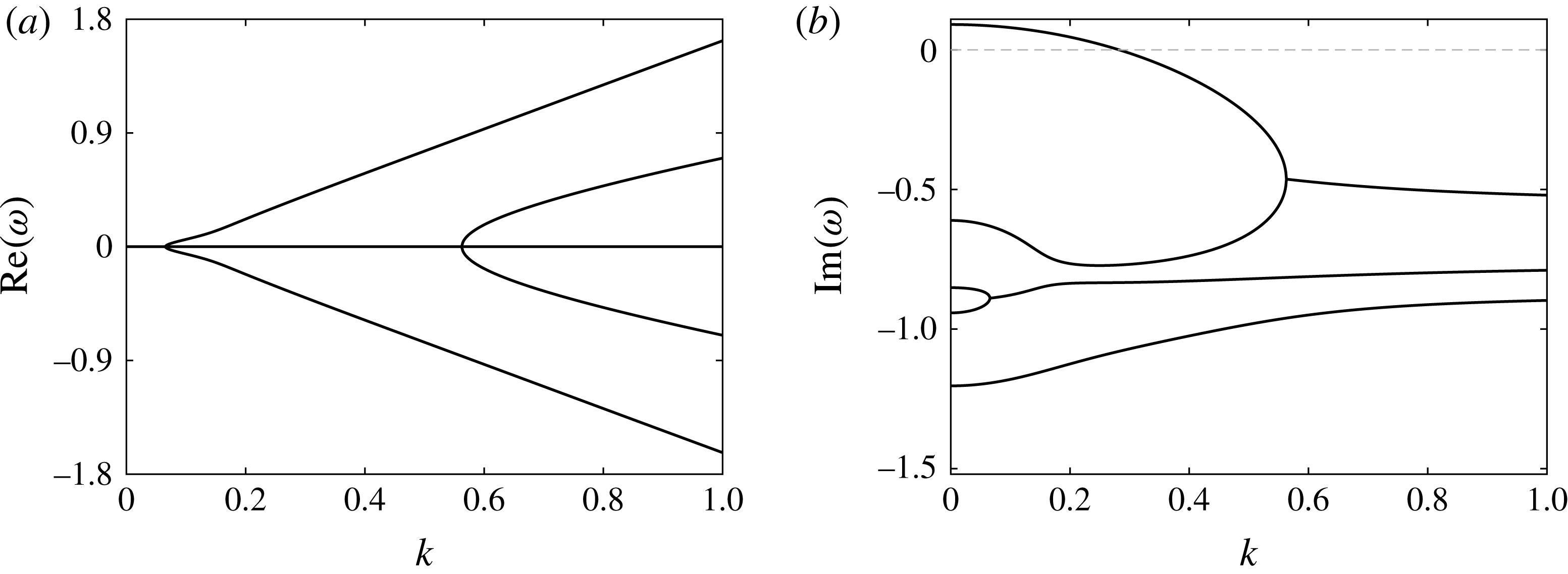
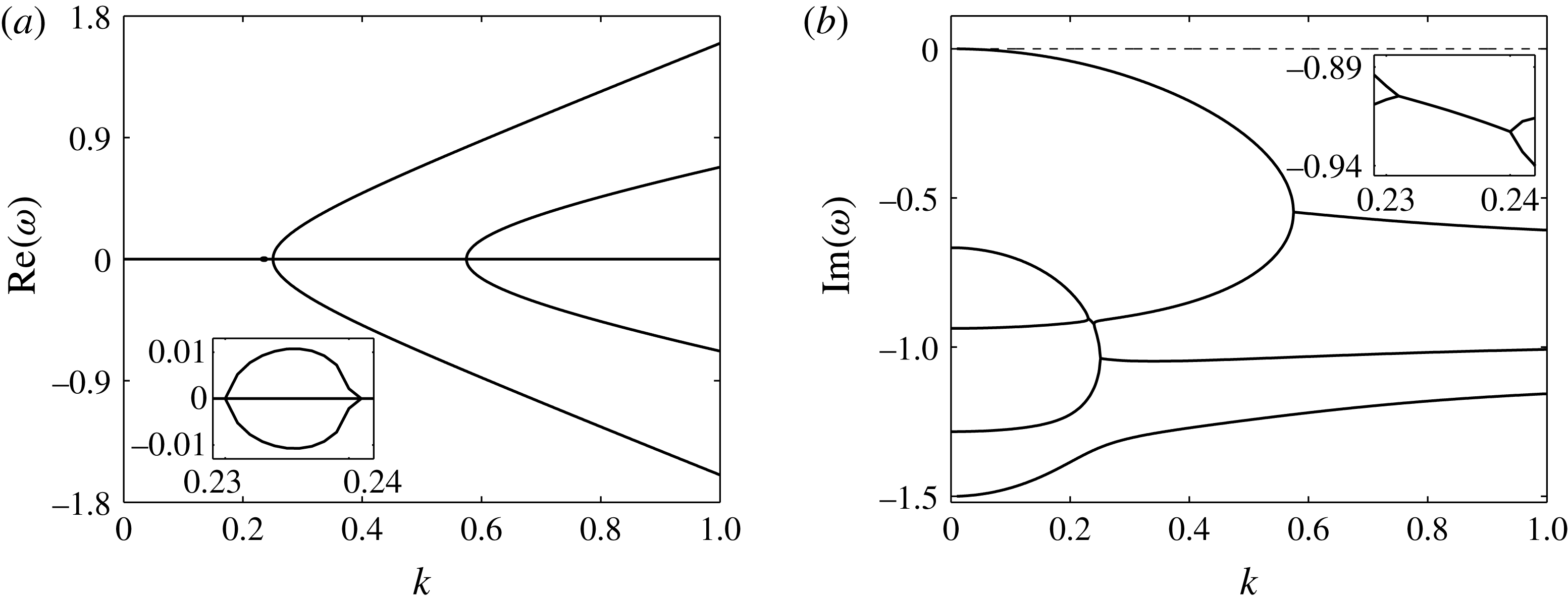
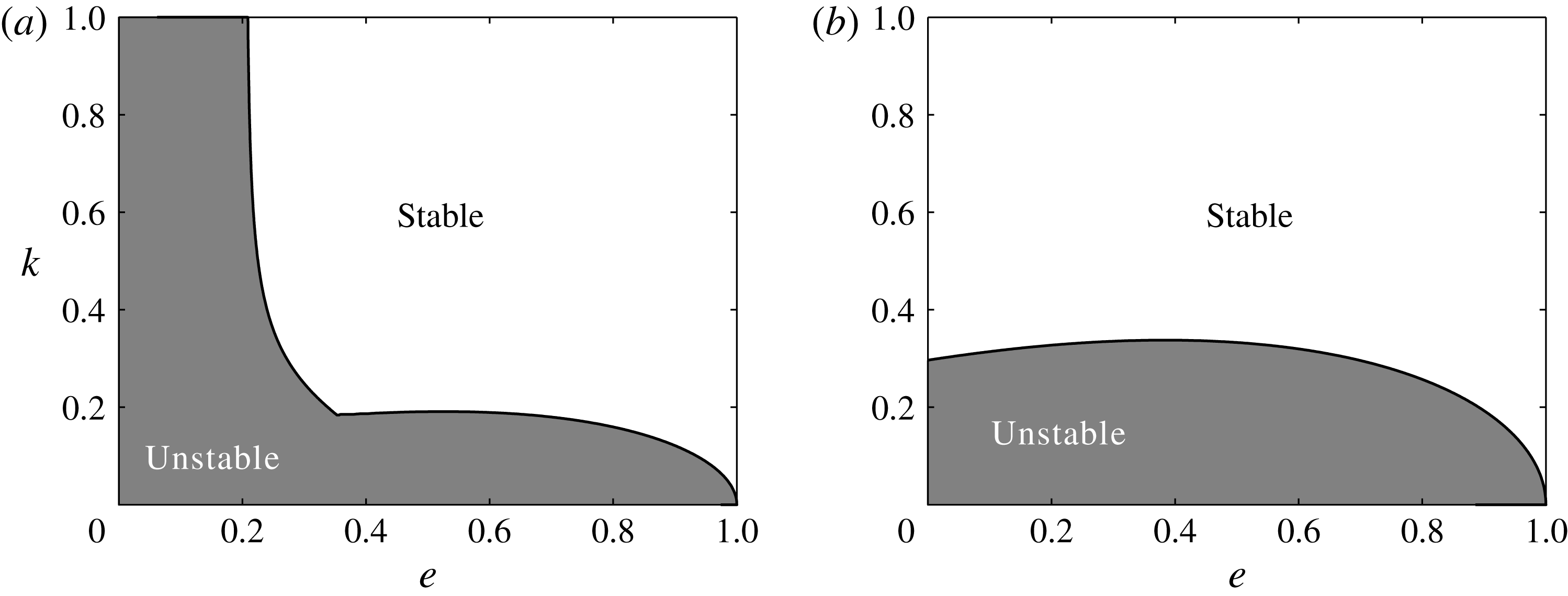
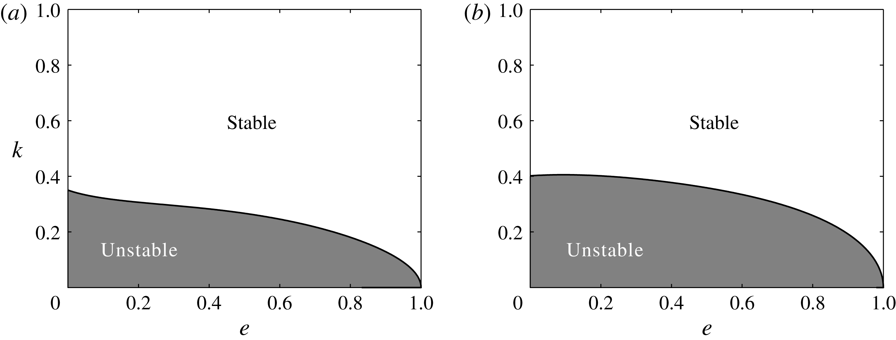
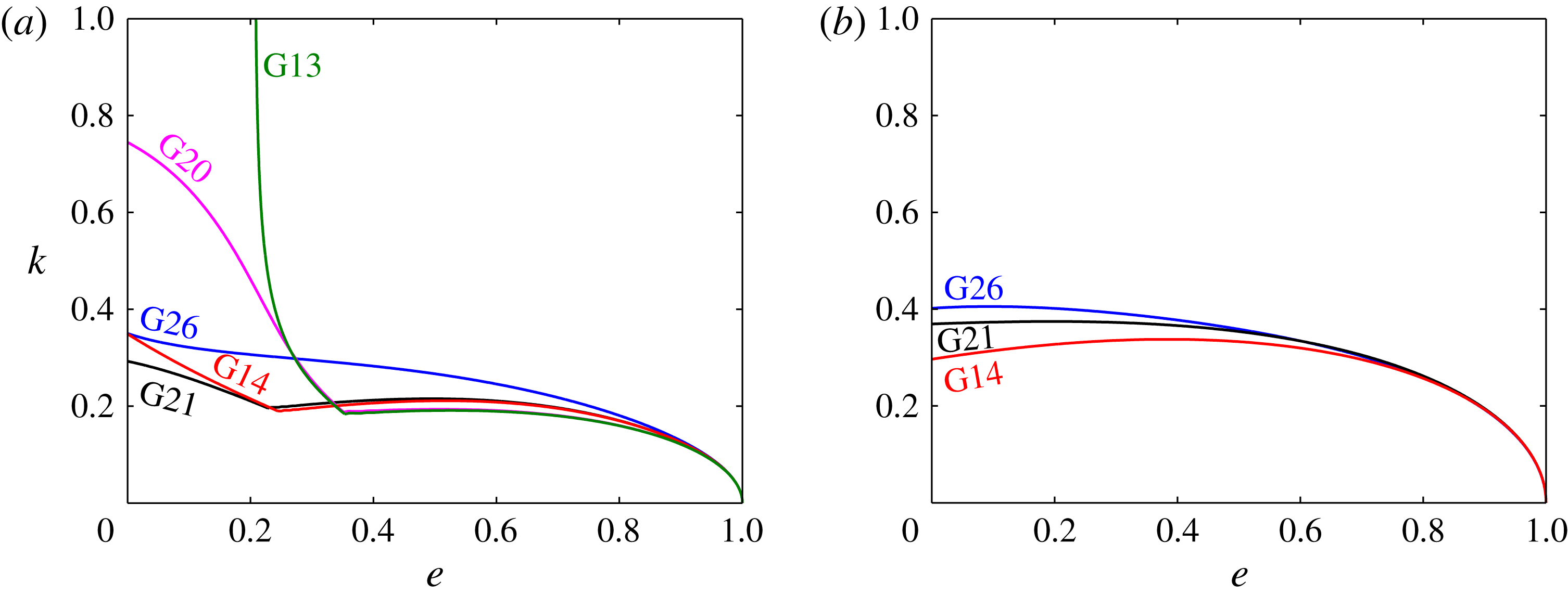
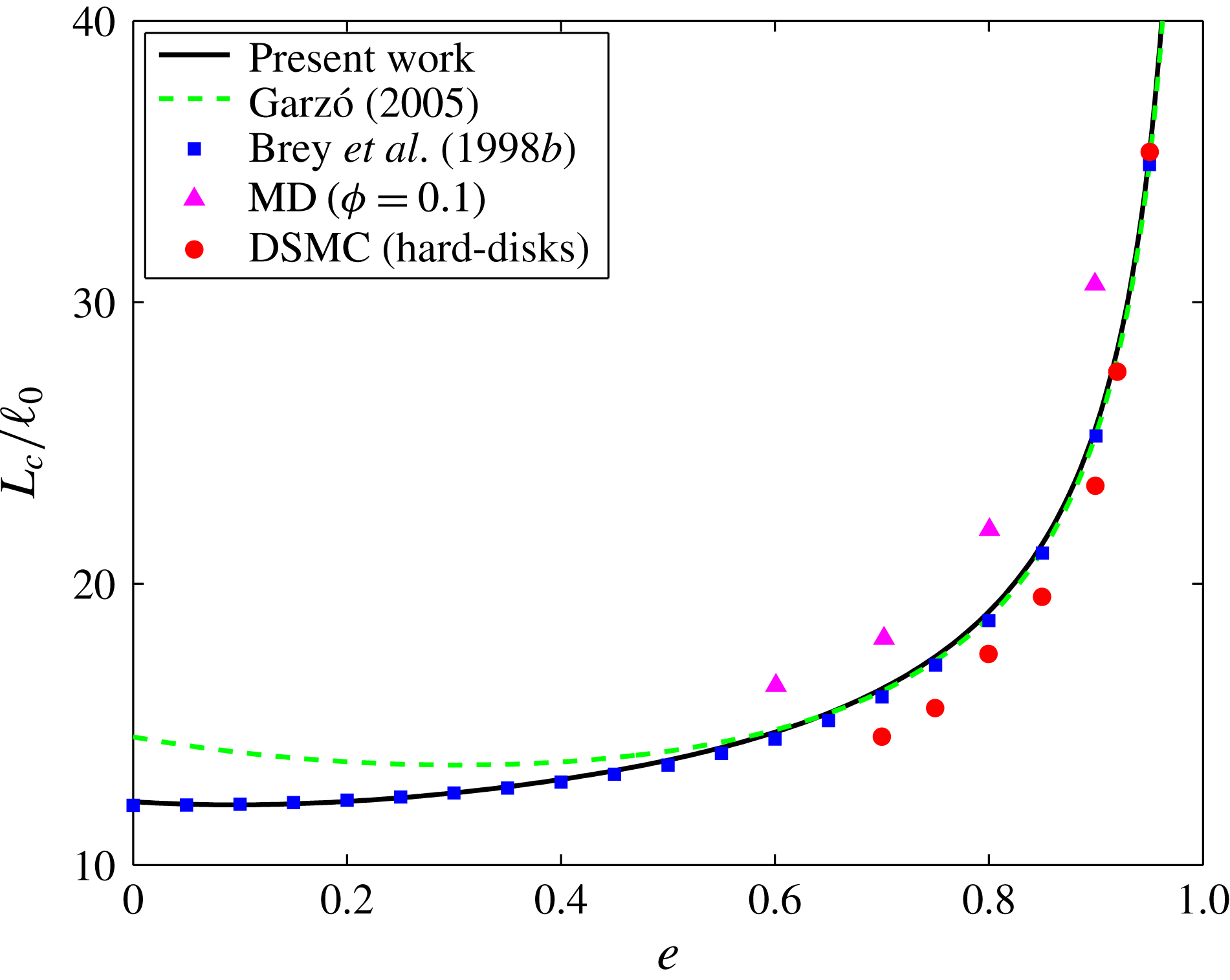
® and presented in appendix A for hard-sphere interaction potential. The production terms for the G26 equations can readily be found from those for the G27 equations by simply discarding the terms containing the fully contracted sixth moment. Here, it is noteworthy to point out that the present work does not have any restriction on the coefficient of restitution other than being a constant, and is, consequently, expected to be applicable not only for nearly elastic granular gases but also for those having large inelasticity. With the semi-linearized G26 and G27 equations, we investigate the HCS – which has also been studied a great deal theoretically, numerically as well as experimentally – of a freely cooling granular gas to show that the decay of the granular temperature closely follows Haff’s law (Haff Reference Haff1983) while the other higher-order moments relax on a faster time scale than the granular temperature. We further study the effect of nonlinear terms of the scalar fourth moment and that of linear terms of the scalar sixth moment on Haff’s law. Following the approach of Garzó (Reference Garzó2013), we determine the constitutive relations for the stress and heat flux for dilute granular gases through the G26 equations and compare them with those obtained via the CE expansion and via computer simulations. We further investigate the linear stability of the HCS by scrutinizing the eigenmodes of longitudinal and transverse problems associated with the G26 system and other subsystems. Similar problems related to the stability of eigenmodes have been investigated earlier by Brey et al. (Reference Brey, Moreno and Dufty1996) for five-moment theory and by Kremer & Marques Jr (Reference Kremer and Marques2011) for 13-moment theory. We find that one eigenmode from each Grad moment theory considered in this paper is unstable for inelastic gases while the others are stable, while all of the eigenmodes are stable for monatomic (elastic) gases. Moreover, the 13-moment theory of Kremer & Marques Jr (Reference Kremer and Marques2011) shows that the unstable heat mode of the longitudinal system remains unstable below a certain value of the coefficient of restitution for all wavenumbers, while the present work reveals that the unstable heat mode of the longitudinal system associated with all moment theories expect for the G13 theory becomes stable above a critical wavenumber for all values of the coefficient of restitution. By investigating the critical wavenumbers of the longitudinal and transverse systems from the G26 theory, we also study the critical system size, beyond which the system becomes unstable, and compare the results with existing theories and simulations. The findings of this paper will be useful for a better understanding of granular gases, for the development of new mathematical models – such as regularized moment equations – and boundary conditions, and for capturing some intriguing features of granular gases theoretically.
The rest of the paper is structured as follows. Kinetic theory for granular gases is briefly reviewed in § 2. Grad’s method of moments is outlined and applied to derive the Grad moment systems of various orders – in particular, the system of G26 equations – for granular gases in § 3. The HCS of a freely cooling granular gas is investigated through the G26 and G27 equations in § 4 in order to discern the effects of nonlinear terms of the scalar fourth moment and of linear terms of the scalar sixth moment on the HCS. The constitutive relations for the stress and heat flux are computed through the G26 equations in § 5. The linear stability of the HCS is analysed in § 6 through the G26 equations by decomposing them into longitudinal and transverse systems. The conclusions are given in § 7.
2 Short review of kinetic theory
We consider a dilute granular gas composed of smooth inelastic identical hard spheres of mass
 $m$
and diameter
 $d$
. The binary collision between two such spheres with pre-collisional velocities
 $\boldsymbol{c}$
and
 $\boldsymbol{c}_{1}$
leads to the following velocity transformation after the collision (see, e.g., Brilliantov & Pöschel Reference Brilliantov and Pöschel2004; Rao & Nott Reference Rao and Nott2008):
 $$\begin{eqnarray}\left.\begin{array}{@{}c@{}}\displaystyle \boldsymbol{c}^{\prime }=\boldsymbol{c}-\frac{1+e}{2}(\hat{\boldsymbol{k}}\boldsymbol{\cdot }\boldsymbol{g})\hat{\boldsymbol{k}},\\ \displaystyle \boldsymbol{c}_{1}^{\prime }=\boldsymbol{c}_{1}+\frac{1+e}{2}(\hat{\boldsymbol{k}}\boldsymbol{\cdot }\boldsymbol{g})\hat{\boldsymbol{k}},\end{array}\right\}\end{eqnarray}$$
where
 $\boldsymbol{c}^{\prime }$
and
 $\boldsymbol{c}_{1}^{\prime }$
are the post-collisional velocities of the respective spheres,
 $\boldsymbol{g}=\boldsymbol{c}-\boldsymbol{c}_{1}$
is the relative velocity,
 $\hat{\boldsymbol{k}}$
is the unit vector directed from the centre of one sphere to that of other at the time of collision and
 $e$
is the coefficient of normal restitution (also referred to as the coefficient of restitution). The coefficient of restitution
 $e$
, in principle, is not a constant and usually depends on the impact velocity (Bizon et al.
Reference Bizon, Shattuck, Swift and Swinney1999; Brilliantov & Pöschel Reference Brilliantov and Pöschel2004). Nevertheless, for simplicity, we assume that
 $e$
is constant with
 $0\leqslant e\leqslant 1$
in this work. The two limiting cases of
 $e=0$
and
 $e=1$
correspond to sticky and perfectly elastic collisions respectively.
In kinetic theory, the state of a dilute granular gas can be described with the single-particle velocity distribution function
 $f\equiv f(t,\boldsymbol{x},\boldsymbol{c})$
, which obeys the (inelastic) Boltzmann equation (Goldshtein & Shapiro Reference Goldshtein and Shapiro1995; Sela & Goldhirsch Reference Sela and Goldhirsch1998; Brilliantov & Pöschel Reference Brilliantov and Pöschel2004)
 $$\begin{eqnarray}\frac{\unicode[STIX]{x2202}f}{\unicode[STIX]{x2202}t}+c_{i}\,\frac{\unicode[STIX]{x2202}f}{\unicode[STIX]{x2202}x_{i}}+F_{i}\,\frac{\unicode[STIX]{x2202}f}{\unicode[STIX]{x2202}c_{i}}=d^{2}\int _{\mathbb{R}^{3}}\!\int _{S^{2}}\!\left(\frac{1}{e^{2}}f^{\prime \prime }f_{1}^{\prime \prime }-f\,f_{1}\right)(\hat{\boldsymbol{k}}\boldsymbol{\cdot }\boldsymbol{g})\,\unicode[STIX]{x1D6E9}(\hat{\boldsymbol{k}}\boldsymbol{\cdot }\boldsymbol{g})\,\text{d}\hat{\boldsymbol{k}}\,\text{d}\boldsymbol{c}_{1},\end{eqnarray}$$
where
 $\unicode[STIX]{x1D6E9}$
is the Heaviside step function,
 $\boldsymbol{F}$
is the external force per unit mass and usually does not depend on
 $\boldsymbol{c}$
,
 $f_{1}\equiv f(t,\boldsymbol{x},\boldsymbol{c}_{1})$
,
 $f^{\prime \prime }\equiv f(t,\boldsymbol{x},\boldsymbol{c}^{\prime \prime })$
,
 $f_{1}^{\prime \prime }\equiv f(t,\boldsymbol{x},\boldsymbol{c}_{1}^{\prime \prime })$
, the integration limits of
 $\hat{\boldsymbol{k}}$
extend over the unit sphere
 $S^{2}$
and the Einstein summation convention is assumed over repeated indices. The velocities
 $\boldsymbol{c}^{\prime \prime }$
and
 $\boldsymbol{c}_{1}^{\prime \prime }$
are the pre-collisional velocities in an inverse collision and are related to
 $\boldsymbol{c}$
and
 $\boldsymbol{c}_{1}$
as follows (see, e.g., Brilliantov & Pöschel Reference Brilliantov and Pöschel2004; Rao & Nott Reference Rao and Nott2008):
 $$\begin{eqnarray}\left.\begin{array}{@{}c@{}}\displaystyle \boldsymbol{c}^{\prime \prime }=\boldsymbol{c}-\frac{1+e}{2e}(\hat{\boldsymbol{k}}\boldsymbol{\cdot }\boldsymbol{g})\hat{\boldsymbol{k}},\\ \displaystyle \boldsymbol{c}_{1}^{\prime \prime }=\boldsymbol{c}_{1}+\frac{1+e}{2e}(\hat{\boldsymbol{k}}\boldsymbol{\cdot }\boldsymbol{g})\hat{\boldsymbol{k}}.\end{array}\right\}\end{eqnarray}$$
For the sake of brevity, hereafter, we shall omit the limits of integrations. Nevertheless, the integration over any velocity space will stand for the volume integral over
 $\mathbb{R}^{3}$
and that over
 $\hat{\boldsymbol{k}}$
will stand for the volume integral over the unit sphere
 $S^{2}$
. The right-hand side of (2.2) is referred to as the (inelastic) Boltzmann collision operator.
The hydrodynamic variables – number density
 $n\equiv n(t,\boldsymbol{x})$
, macroscopic velocity
 $\boldsymbol{v}\equiv \boldsymbol{v}(t,\boldsymbol{x})$
, granular temperature
 $T\equiv T(t,\boldsymbol{x})$
– are directly related to the velocity distribution function as follows:
 $$\begin{eqnarray}\displaystyle & \displaystyle n(t,\boldsymbol{x})=\int f(t,\boldsymbol{x},\boldsymbol{c})\,\text{d}\boldsymbol{c}, & \displaystyle\end{eqnarray}$$
 $$\begin{eqnarray}\displaystyle & \displaystyle n(t,\boldsymbol{x})\boldsymbol{v}(t,\boldsymbol{x})=\int \boldsymbol{c}f(t,\boldsymbol{x},\boldsymbol{c})\,\text{d}\boldsymbol{c}, & \displaystyle\end{eqnarray}$$
 $$\begin{eqnarray}\displaystyle & \displaystyle \frac{3}{2}n(t,\boldsymbol{x})T(t,\boldsymbol{x})=\frac{1}{2}m\int C^{2}f(t,\boldsymbol{x},\boldsymbol{c})\,\text{d}\boldsymbol{c}, & \displaystyle\end{eqnarray}$$
where
 $\boldsymbol{C}(t,\boldsymbol{x},\boldsymbol{c})=\boldsymbol{c}-\boldsymbol{v}(t,\boldsymbol{x})$
is the peculiar velocity. Here, the definition of the granular temperature – which is a measure of the fluctuating kinetic energy – is adopted following Brilliantov & Pöschel (Reference Brilliantov and Pöschel2004) and Garzó (Reference Garzó2013), although some authors, for instance Lun et al. (Reference Lun, Savage, Jeffrey and Chepurniy1984), Campbell (Reference Campbell1990) and Saha & Alam (Reference Saha and Alam2014), also refer to
 $\unicode[STIX]{x1D703}=T/m$
as the granular temperature (defined as the fluctuating kinetic energy per unit mass). It should be noted that in the case of monatomic gases,
 $T$
in (2.6) is replaced with
 $k_{B}T_{th}$
, where
 $k_{B}$
denotes the Boltzmann constant and
 $T_{th}$
is the thermodynamic temperature.
The governing equations for the hydrodynamic variables can be derived from the Boltzmann equation (2.2) as follows. Let us first introduce the moments. For a particle property,
 $\unicode[STIX]{x1D713}\equiv \unicode[STIX]{x1D713}(t,\boldsymbol{x},\boldsymbol{c})$
, its average value
 $\langle \unicode[STIX]{x1D713}\rangle \equiv \langle \unicode[STIX]{x1D713}\rangle (t,\boldsymbol{x})$
is defined in terms of the distribution function
 $f$
as
 $$\begin{eqnarray}\langle \unicode[STIX]{x1D713}\rangle (t,\boldsymbol{x})=\frac{1}{n(t,\boldsymbol{x})}\int \unicode[STIX]{x1D713}(t,\boldsymbol{x},\boldsymbol{c})\,f(t,\boldsymbol{x},\boldsymbol{c})\,\text{d}\boldsymbol{c}.\end{eqnarray}$$
The integral
 $\int \unicode[STIX]{x1D713}f\,\text{d}\boldsymbol{c}$
on the right-hand side of (2.7) is referred to as the moment of the velocity distribution function with respect to
 $\unicode[STIX]{x1D713}$
. Clearly,
 $$\begin{eqnarray}1=\langle 1\rangle ,\quad \boldsymbol{v}=\langle \boldsymbol{c}\rangle \quad \text{and}\quad T=\left\langle {\textstyle \frac{1}{3}}mC^{2}\right\rangle .\end{eqnarray}$$
The governing equation for the moment
 $\int \unicode[STIX]{x1D713}f\,\text{d}\boldsymbol{c}$
– often referred to as the moment equation for
 $n\langle \unicode[STIX]{x1D713}\rangle$
or the transfer equation for property
 $\unicode[STIX]{x1D713}$
– is obtained by multiplying the Boltzmann equation (2.2) with
 $\unicode[STIX]{x1D713}$
and integrating over the velocity space
 $\boldsymbol{c}$
. The transfer equation for the quantity
 $\unicode[STIX]{x1D713}$
reads
 $$\begin{eqnarray}\frac{\text{D}}{\text{D}t}\!\int \unicode[STIX]{x1D713}f\,\text{d}\boldsymbol{c}+\text{}\underline{\frac{\unicode[STIX]{x2202}}{\unicode[STIX]{x2202}x_{i}}\!\int \unicode[STIX]{x1D713}\,C_{i}\,f\,\text{d}\boldsymbol{c}}+\frac{\unicode[STIX]{x2202}v_{i}}{\unicode[STIX]{x2202}x_{i}}\!\int \unicode[STIX]{x1D713}f\,\text{d}\boldsymbol{c}-\int \left(\frac{\text{D}\unicode[STIX]{x1D713}}{\text{D}t}+C_{i}\frac{\unicode[STIX]{x2202}\unicode[STIX]{x1D713}}{\unicode[STIX]{x2202}x_{i}}+F_{i}\frac{\unicode[STIX]{x2202}\unicode[STIX]{x1D713}}{\unicode[STIX]{x2202}c_{i}}\right)f\,\text{d}\boldsymbol{c}={\mathcal{P}}(\unicode[STIX]{x1D713}),\end{eqnarray}$$
where
 $\text{D}/\text{D}t\equiv \unicode[STIX]{x2202}/\unicode[STIX]{x2202}t+\boldsymbol{v}\boldsymbol{\cdot }\unicode[STIX]{x1D735}$
is the material derivative, the underline denotes the flux term and
 $$\begin{eqnarray}\displaystyle {\mathcal{P}}(\unicode[STIX]{x1D713}) & = & \displaystyle \frac{d^{2}}{2}\iiint \!\big(\unicode[STIX]{x1D713}^{\prime }+\unicode[STIX]{x1D713}_{1}^{\prime }-\unicode[STIX]{x1D713}-\unicode[STIX]{x1D713}_{1}\big)f\,f_{1}(\hat{\boldsymbol{k}}\boldsymbol{\cdot }\boldsymbol{g})\unicode[STIX]{x1D6E9}(\hat{\boldsymbol{k}}\boldsymbol{\cdot }\boldsymbol{g})\,\text{d}\hat{\boldsymbol{k}}\,\text{d}\boldsymbol{c}\,\text{d}\boldsymbol{c}_{1}\nonumber\\ \displaystyle & = & \displaystyle d^{2}\iiint \big(\unicode[STIX]{x1D713}^{\prime }-\unicode[STIX]{x1D713}\big)\,f\,f_{1}(\hat{\boldsymbol{k}}\boldsymbol{\cdot }\boldsymbol{g})\unicode[STIX]{x1D6E9}(\hat{\boldsymbol{k}}\boldsymbol{\cdot }\boldsymbol{g})\,\text{d}\hat{\boldsymbol{k}}\,\text{d}\boldsymbol{c}\,\text{d}\boldsymbol{c}_{1},\end{eqnarray}$$
with
 $\unicode[STIX]{x1D713}^{\prime }\equiv \unicode[STIX]{x1D713}(t,\boldsymbol{x},\boldsymbol{c}^{\prime })$
, etc., is the rate of change of
 $\langle \unicode[STIX]{x1D713}\rangle$
per unit volume due to collisions and is referred to as the production term or the (inelastic) Boltzmann collision integral corresponding to the moment
 $\int \unicode[STIX]{x1D713}f\,\text{d}\boldsymbol{c}$
. In writing (2.10), the symmetry properties of the Boltzmann collision operator (Brilliantov & Pöschel Reference Brilliantov and Pöschel2004; Rao & Nott Reference Rao and Nott2008) have been employed. It should be noted from the transfer equation (2.9) that, irrespective of the value of
 $\unicode[STIX]{x1D713}$
chosen for defining a moment by (2.7), the transfer equation (2.9) will always contain an additional moment of one more order in the flux term. On substituting
 $\unicode[STIX]{x1D713}$
in (2.9) with
 $1$
,
 $c_{i}$
and
 $(1/3)m\,C^{2}$
successively, we get the mass, momentum and energy balance equations respectively, which read
 $$\begin{eqnarray}\displaystyle & \displaystyle \frac{\text{D}n}{\text{D}t}+n\frac{\unicode[STIX]{x2202}v_{i}}{\unicode[STIX]{x2202}x_{i}}=0, & \displaystyle\end{eqnarray}$$
 $$\begin{eqnarray}\displaystyle & \displaystyle \frac{\text{D}v_{i}}{\text{D}t}+\frac{1}{mn}\left[\frac{\unicode[STIX]{x2202}\unicode[STIX]{x1D70E}_{ij}}{\unicode[STIX]{x2202}x_{j}}+\frac{\unicode[STIX]{x2202}(nT)}{\unicode[STIX]{x2202}x_{i}}\right]-F_{i}=0, & \displaystyle\end{eqnarray}$$
 $$\begin{eqnarray}\displaystyle & \displaystyle \frac{\text{D}T}{\text{D}t}+\frac{2}{3n}\left[\frac{\unicode[STIX]{x2202}q_{i}}{\unicode[STIX]{x2202}x_{i}}+\unicode[STIX]{x1D70E}_{ij}\frac{\unicode[STIX]{x2202}v_{i}}{\unicode[STIX]{x2202}x_{j}}+nT\frac{\unicode[STIX]{x2202}v_{i}}{\unicode[STIX]{x2202}x_{i}}\right]=-\unicode[STIX]{x1D701}T. & \displaystyle\end{eqnarray}$$
In (2.12) and (2.13),
 $\unicode[STIX]{x1D70E}_{ij}\equiv \unicode[STIX]{x1D70E}_{ij}(t,\boldsymbol{x})$
and
 $q_{i}\equiv q_{i}(t,\boldsymbol{x})$
are the components of the stress tensor and heat flux respectively, and, following the notations of Struchtrup (Reference Struchtrup2005), these are given by
 $$\begin{eqnarray}\unicode[STIX]{x1D70E}_{ij}=m\int C_{\langle \!i}C_{j\!\rangle }\,f\,\text{d}\boldsymbol{c}\quad \text{and}\quad q_{i}=\frac{1}{2}m\int C^{2}C_{i}\,f\,\text{d}\boldsymbol{c},\end{eqnarray}$$
where the angle brackets around the indices denote the symmetric and traceless part of the tensor (Struchtrup Reference Struchtrup2005), and
 $\unicode[STIX]{x1D701}$
in (2.13) is the cooling rate due to inelastic collisions:
 $$\begin{eqnarray}\unicode[STIX]{x1D701}=-\frac{m\,d^{2}}{6\,n\,T}\iiint \left((C^{\prime })^{2}+(C_{1}^{\prime })^{2}-C^{2}-C_{1}^{2}\right)f\,f_{1}(\hat{\boldsymbol{k}}\boldsymbol{\cdot }\boldsymbol{g})\unicode[STIX]{x1D6E9}(\hat{\boldsymbol{k}}\boldsymbol{\cdot }\boldsymbol{g})\,\text{d}\hat{\boldsymbol{k}}\,\text{d}\boldsymbol{c}\,\text{d}\boldsymbol{c}_{1}.\end{eqnarray}$$
It should be noted that the right-hand sides of (2.11) and (2.12) vanish due to conservation of mass and momentum; however, the energy is not conserved due to dissipative collisions resulting in a non-vanishing right-hand side in (2.13). It is worth pointing out that the stress and heat flux appearing in (2.12) and (2.13), in general, have non-vanishing collisional contributions in addition to the usual kinetic contribution given by (2.14) (Brey, Dufty & Santos Reference Brey, Dufty and Santos1997; Garzó & Dufty Reference Garzó and Dufty1999; Rao & Nott Reference Rao and Nott2008; Garzó Reference Garzó2013). However, for dilute granular gases, the kinetic contributions to the stress and heat flux dominate over their respective collisional transfer contributions, and therefore the collisional transfer contributions to the stress and heat flux can be neglected for dilute granular gases (Brilliantov & Pöschel Reference Brilliantov and Pöschel2004). In any case, since (2.12) and (2.13) are obtained here by taking the velocity moments of the distribution function, which is essentially the idea of Grad’s method of moments too, only kinetic contributions to the stress and heat flux will emerge in the equations. The collisional contributions to the stress and heat flux, in the case of dense granular gases, must be computed separately (Garzó Reference Garzó2013).
Obviously, the system of equations (2.11)–(2.13) in the hydrodynamic variables
 $n$
,
 $v_{i}$
and
 $T$
is not closed, since it contains the unknowns
 $\unicode[STIX]{x1D70E}_{ij}$
,
 $q_{i}$
and
 $\unicode[STIX]{x1D701}$
, and in order to deal with this system further one must close it. Here, we employ Grad’s method of moments (Grad Reference Grad1949b
) in order to obtain a closed system of equations.
3 Grad’s method of moments
The function
 $\unicode[STIX]{x1D713}$
in (2.7) can be chosen in infinitely many ways. Therefore, the transfer equation (2.9) leads to an infinite hierarchy of moment equations. However, in practice, only a finite number of moment equations, obtained by truncating the infinite hierarchy of moment equations at a certain level, are used. Nonetheless, this truncated system of equations is not closed due to the (underlined) flux term in (2.9). In order to obtain a closed (finite) system of moment equations, Grad (Reference Grad1949b
) expanded the velocity distribution function
 $f$
in a finite linear combination of the
 $N$
-dimensional Hermite polynomials (Grad Reference Grad1949a
) in peculiar velocity and computed the unknown coefficients in the expansion in terms of the considered moments by satisfying their definitions with the approximated distribution function. This method of obtaining a closed set of moment equations is referred to as Grad’s method of moments and its details can be found in Grad (Reference Grad1949b
) and many standard textbooks; see, e.g., Struchtrup (Reference Struchtrup2005) and Kremer (Reference Kremer2010).
On including the governing equations for stress (
 $\unicode[STIX]{x1D70E}_{ij}$
) and heat flux (
 $q_{i}$
) in the system of mass, momentum and energy balance equations (2.11)–(2.13), one obtains the well-known 13-moment equations (in three dimensions). Here, we want to derive and explore the G26 equations for dilute granular flows. To this end, let us first introduce the general form of a moment. The typical form of
 $\unicode[STIX]{x1D713}$
is
 $m\,C^{2a}C_{\langle \!i_{1}}C_{i_{2}}\ldots C_{i_{n}\!\rangle }$
, where
 $a,n\in \mathbb{N}_{0}$
and the angle brackets around the indices again denote the symmetric and traceless part of the corresponding quantity (Struchtrup Reference Struchtrup2005). Thus, a general moment is given by
 $$\begin{eqnarray}u_{i_{1}i_{2}\ldots i_{n}}^{a}=m\int C^{2a}C_{\langle \!i_{1}}C_{i_{2}}\ldots C_{i_{n}\!\rangle }\,f\,\text{d}\boldsymbol{c},\quad a,n\in \mathbb{N}_{0}.\end{eqnarray}$$
Clearly,
 $$\begin{eqnarray}u^{0}=m\,n=\unicode[STIX]{x1D70C},\quad u_{i}^{0}=0,\quad u^{1}=3\,nT=3\unicode[STIX]{x1D70C}\unicode[STIX]{x1D703},\quad u_{ij}^{0}=\unicode[STIX]{x1D70E}_{ij},\quad u_{i}^{1}=2q_{i},\end{eqnarray}$$
where
 $\unicode[STIX]{x1D70C}=m\,n$
is the mass density and
 $\unicode[STIX]{x1D703}=T/m$
.
3.1 The 26-moment equations
In addition to the well-known 13 moments, the system of 26-moment equations includes the full third rank tensor and one and full traces of the fourth moment (i.e. the 26-moment equations include the moments
 $n$
,
 $v_{i}$
,
 $T$
,
 $\unicode[STIX]{x1D70E}_{ij}$
,
 $q_{i}$
,
 $u_{ijk}^{0}$
,
 $u_{ij}^{1}$
,
 $u^{2}$
). The system of G26 equations is obtained by substituting
 $\unicode[STIX]{x1D713}$
in (2.9) with
 $1$
,
 $c_{i}$
,
 $(1/3)m\,C^{2}$
,
 $m\,C_{\langle \!i}C_{j\!\rangle }$
,
 $(1/2)m\,C^{2}C_{i}$
,
 $m\,C_{\langle \!i}C_{j}C_{k\!\rangle }$
,
 $m\,C^{2}C_{\langle \!i}C_{j\!\rangle }$
and
 $m\,C^{4}$
successively. The system of 26-moment equations consists of the mass, momentum and energy balance equations (2.11)–(2.13) and other higher-order moment equations, which, on using the abbreviations
 $$\begin{eqnarray}m_{ijk}=u_{ijk}^{0},\quad R_{ij}=u_{ij}^{1}-7\unicode[STIX]{x1D703}\unicode[STIX]{x1D70E}_{ij},\quad w=u^{2}-15\unicode[STIX]{x1D70C}\unicode[STIX]{x1D703}^{2},\end{eqnarray}$$
read
 $$\begin{eqnarray}\displaystyle & & \displaystyle \displaystyle \frac{\text{D}\unicode[STIX]{x1D70E}_{ij}}{\text{D}t}+\frac{\unicode[STIX]{x2202}m_{ijk}}{\unicode[STIX]{x2202}x_{k}}+\frac{4}{5}\frac{\unicode[STIX]{x2202}q_{\langle \!i}}{\unicode[STIX]{x2202}x_{j\!\rangle }}+\unicode[STIX]{x1D70E}_{ij}\frac{\unicode[STIX]{x2202}v_{k}}{\unicode[STIX]{x2202}x_{k}}+2\unicode[STIX]{x1D70E}_{k\langle i}\frac{\unicode[STIX]{x2202}v_{j\!\rangle }}{\unicode[STIX]{x2202}x_{k}}+2\unicode[STIX]{x1D70C}\unicode[STIX]{x1D703}\frac{\unicode[STIX]{x2202}v_{\langle \!i}}{\unicode[STIX]{x2202}x_{j\!\rangle }}={\mathcal{P}}_{ij}^{0},\end{eqnarray}$$
 $$\begin{eqnarray}\displaystyle & & \displaystyle \displaystyle \frac{\text{D}q_{i}}{\text{D}t}+\frac{1}{2}\frac{\unicode[STIX]{x2202}R_{ij}}{\unicode[STIX]{x2202}x_{j}}+\frac{1}{6}\frac{\unicode[STIX]{x2202}w}{\unicode[STIX]{x2202}x_{i}}+\unicode[STIX]{x1D703}\frac{\unicode[STIX]{x2202}\unicode[STIX]{x1D70E}_{ij}}{\unicode[STIX]{x2202}x_{j}}+\frac{5}{2}\unicode[STIX]{x1D70E}_{ij}\frac{\unicode[STIX]{x2202}\unicode[STIX]{x1D703}}{\unicode[STIX]{x2202}x_{j}}+\frac{5}{2}\unicode[STIX]{x1D70C}\unicode[STIX]{x1D703}\frac{\unicode[STIX]{x2202}\unicode[STIX]{x1D703}}{\unicode[STIX]{x2202}x_{i}}+m_{ijk}\frac{\unicode[STIX]{x2202}v_{j}}{\unicode[STIX]{x2202}x_{k}}\nonumber\\ \displaystyle & & \displaystyle \quad -\,\unicode[STIX]{x1D70E}_{ij}\frac{1}{\unicode[STIX]{x1D70C}}\left(\frac{\unicode[STIX]{x2202}\unicode[STIX]{x1D70E}_{jk}}{\unicode[STIX]{x2202}x_{k}}+\unicode[STIX]{x1D703}\frac{\unicode[STIX]{x2202}\unicode[STIX]{x1D70C}}{\unicode[STIX]{x2202}x_{j}}\right)+\frac{7}{5}q_{i}\frac{\unicode[STIX]{x2202}v_{j}}{\unicode[STIX]{x2202}x_{j}}+\frac{7}{5}q_{j}\frac{\unicode[STIX]{x2202}v_{i}}{\unicode[STIX]{x2202}x_{j}}+\frac{2}{5}q_{j}\frac{\unicode[STIX]{x2202}v_{j}}{\unicode[STIX]{x2202}x_{i}}=\frac{1}{2}{\mathcal{P}}_{i}^{1},\end{eqnarray}$$
 $$\begin{eqnarray}\displaystyle & & \displaystyle \displaystyle \frac{\text{D}m_{ijk}}{\text{D}t}+\frac{\unicode[STIX]{x2202}u_{ijkl}^{0}}{\unicode[STIX]{x2202}x_{l}}+\frac{3}{7}\frac{\unicode[STIX]{x2202}R_{\langle \!ij}}{\unicode[STIX]{x2202}x_{k\!\rangle }}+3\unicode[STIX]{x1D703}\frac{\unicode[STIX]{x2202}\unicode[STIX]{x1D70E}_{\langle \!ij}}{\unicode[STIX]{x2202}x_{k\!\rangle }}-3\frac{1}{\unicode[STIX]{x1D70C}}\unicode[STIX]{x1D70E}_{\langle \!ij}\left(\frac{\unicode[STIX]{x2202}\unicode[STIX]{x1D70E}_{k\rangle l}}{\unicode[STIX]{x2202}x_{l}}+\unicode[STIX]{x1D703}\frac{\unicode[STIX]{x2202}\unicode[STIX]{x1D70C}}{\unicode[STIX]{x2202}x_{k\!\rangle }}\right)\nonumber\\ \displaystyle & & \displaystyle \quad +\,m_{ijk}\frac{\unicode[STIX]{x2202}v_{l}}{\unicode[STIX]{x2202}x_{l}}+3m_{l\langle ij}\frac{\unicode[STIX]{x2202}v_{k\!\rangle }}{\unicode[STIX]{x2202}x_{l}}+\frac{12}{5}q_{\langle \!i}\frac{\unicode[STIX]{x2202}v_{j}}{\unicode[STIX]{x2202}x_{k\!\rangle }}={\mathcal{P}}_{ijk}^{0},\end{eqnarray}$$
 $$\begin{eqnarray}\displaystyle & & \displaystyle \displaystyle \frac{\text{D}R_{ij}}{\text{D}t}+2u_{ijkl}^{0}\frac{\unicode[STIX]{x2202}v_{k}}{\unicode[STIX]{x2202}x_{l}}+\frac{\unicode[STIX]{x2202}u_{ijk}^{1}}{\unicode[STIX]{x2202}x_{k}}+\frac{2}{5}\frac{\unicode[STIX]{x2202}u_{\langle \!i}^{2}}{\unicode[STIX]{x2202}x_{j\!\rangle }}+R_{ij}\frac{\unicode[STIX]{x2202}v_{k}}{\unicode[STIX]{x2202}x_{k}}-\frac{28}{5}\unicode[STIX]{x1D703}\frac{\unicode[STIX]{x2202}q_{\langle \!i}}{\unicode[STIX]{x2202}x_{j\!\rangle }}-\frac{28}{5}q_{\langle \!i}\frac{\unicode[STIX]{x2202}\unicode[STIX]{x1D703}}{\unicode[STIX]{x2202}x_{j\!\rangle }}\nonumber\\ \displaystyle & & \displaystyle \qquad +\,4\unicode[STIX]{x1D703}\displaystyle \unicode[STIX]{x1D70E}_{k\langle i}\frac{\unicode[STIX]{x2202}v_{k}}{\unicode[STIX]{x2202}x_{j\!\rangle }}+4\unicode[STIX]{x1D703}\unicode[STIX]{x1D70E}_{k\langle i}\frac{\unicode[STIX]{x2202}v_{j\!\rangle }}{\unicode[STIX]{x2202}x_{k}}-\frac{8}{3}\unicode[STIX]{x1D703}\unicode[STIX]{x1D70E}_{ij}\frac{\unicode[STIX]{x2202}v_{k}}{\unicode[STIX]{x2202}x_{k}}-\frac{14}{3}\frac{1}{\unicode[STIX]{x1D70C}}\unicode[STIX]{x1D70E}_{ij}\frac{\unicode[STIX]{x2202}q_{k}}{\unicode[STIX]{x2202}x_{k}}-\frac{14}{3}\frac{1}{\unicode[STIX]{x1D70C}}\unicode[STIX]{x1D70E}_{ij}\unicode[STIX]{x1D70E}_{kl}\frac{\unicode[STIX]{x2202}v_{k}}{\unicode[STIX]{x2202}x_{l}}\nonumber\\ \displaystyle & & \displaystyle \qquad \displaystyle -\,7\unicode[STIX]{x1D703}\frac{\unicode[STIX]{x2202}m_{ijk}}{\unicode[STIX]{x2202}x_{k}}+\frac{6}{7}R_{\langle \!ij}\frac{\unicode[STIX]{x2202}v_{k\!\rangle }}{\unicode[STIX]{x2202}x_{k}}+\frac{4}{5}R_{k\langle i}\frac{\unicode[STIX]{x2202}v_{k}}{\unicode[STIX]{x2202}x_{j\!\rangle }}+2R_{k\langle i}\frac{\unicode[STIX]{x2202}v_{j\!\rangle }}{\unicode[STIX]{x2202}x_{k}}+\frac{14}{15}w\frac{\unicode[STIX]{x2202}v_{\langle \!i}}{\unicode[STIX]{x2202}x_{j\!\rangle }}\nonumber\\ \displaystyle & & \displaystyle \qquad \displaystyle -\,2m_{ijk}\frac{\unicode[STIX]{x2202}\unicode[STIX]{x1D703}}{\unicode[STIX]{x2202}x_{k}}-2\frac{1}{\unicode[STIX]{x1D70C}}m_{ijk}\left(\frac{\unicode[STIX]{x2202}\unicode[STIX]{x1D70E}_{kl}}{\unicode[STIX]{x2202}x_{l}}+\unicode[STIX]{x1D703}\frac{\unicode[STIX]{x2202}\unicode[STIX]{x1D70C}}{\unicode[STIX]{x2202}x_{k}}\right)-\frac{28}{5}\frac{1}{\unicode[STIX]{x1D70C}}q_{\langle \!i}\left(\frac{\unicode[STIX]{x2202}\unicode[STIX]{x1D70E}_{j\rangle k}}{\unicode[STIX]{x2202}x_{k}}+\unicode[STIX]{x1D703}\frac{\unicode[STIX]{x2202}\unicode[STIX]{x1D70C}}{\unicode[STIX]{x2202}x_{j\!\rangle }}\right)\nonumber\\ \displaystyle & & \displaystyle \quad \displaystyle ={\mathcal{P}}_{ij}^{1}-7\unicode[STIX]{x1D703}{\mathcal{P}}_{ij}^{0}-\frac{14}{3}\frac{1}{\unicode[STIX]{x1D70C}}\unicode[STIX]{x1D70E}_{ij}\left(\frac{1}{2}{\mathcal{P}}^{1}\right),\end{eqnarray}$$
 $$\begin{eqnarray}\displaystyle & & \displaystyle \displaystyle \frac{\text{D}w}{\text{D}t}+\frac{\unicode[STIX]{x2202}u_{i}^{2}}{\unicode[STIX]{x2202}x_{i}}-20\unicode[STIX]{x1D703}\frac{\unicode[STIX]{x2202}q_{i}}{\unicode[STIX]{x2202}x_{i}}-8q_{i}\frac{\unicode[STIX]{x2202}\unicode[STIX]{x1D703}}{\unicode[STIX]{x2202}x_{i}}+\frac{7}{3}w\frac{\unicode[STIX]{x2202}v_{i}}{\unicode[STIX]{x2202}x_{i}}+4R_{ij}\frac{\unicode[STIX]{x2202}v_{i}}{\unicode[STIX]{x2202}x_{j}}\nonumber\\ \displaystyle & & \displaystyle \quad +\,8\unicode[STIX]{x1D703}\unicode[STIX]{x1D70E}_{ij}\frac{\unicode[STIX]{x2202}v_{i}}{\unicode[STIX]{x2202}x_{j}}-8\frac{1}{\unicode[STIX]{x1D70C}}q_{i}\left(\frac{\unicode[STIX]{x2202}\unicode[STIX]{x1D70E}_{ij}}{\unicode[STIX]{x2202}x_{j}}+\unicode[STIX]{x1D703}\frac{\unicode[STIX]{x2202}\unicode[STIX]{x1D70C}}{\unicode[STIX]{x2202}x_{i}}\right)={\mathcal{P}}^{2}-20\unicode[STIX]{x1D703}\left(\frac{1}{2}{\mathcal{P}}^{1}\right),\end{eqnarray}$$
where
 $$\begin{eqnarray}\displaystyle \displaystyle {\mathcal{P}}_{i_{1}i_{2}\ldots i_{n}}^{a} & = & \displaystyle m\,d^{2}\iiint \!\left((C^{\prime })^{2a}C_{\langle \!i_{1}}^{\prime }C_{i_{2}}^{\prime }\ldots C_{i_{n}\!\rangle }^{\prime }-C^{2a}C_{\langle \!i_{1}}C_{i_{2}}\ldots C_{i_{n}\!\rangle }\right)\nonumber\\ \displaystyle & & \displaystyle \displaystyle \times \,f\,f_{1}(\hat{\boldsymbol{k}}\boldsymbol{\cdot }\boldsymbol{g})\,\unicode[STIX]{x1D6E9}(\hat{\boldsymbol{k}}\boldsymbol{\cdot }\boldsymbol{g})\,\text{d}\hat{\boldsymbol{k}}\,\text{d}\boldsymbol{c}\,\text{d}\boldsymbol{c}_{1}\end{eqnarray}$$
are the production terms. It should be noticed that
 ${\mathcal{P}}^{0}={\mathcal{P}}_{i}^{0}=0$
due to mass and momentum conservation, and
 ${\mathcal{P}}^{1}=-3nT\unicode[STIX]{x1D701}$
.
In (3.3),
 $w$
has been defined as the difference of the full trace of the fourth moment from its value computed with the Maxwellian distribution function
 $$\begin{eqnarray}f_{M}\equiv f_{M}(t,\boldsymbol{x},\boldsymbol{c})=n\left(\frac{1}{2\unicode[STIX]{x03C0}\,\unicode[STIX]{x1D703}}\right)^{3/2}\exp \left(-\frac{C^{2}}{2\unicode[STIX]{x1D703}}\right),\end{eqnarray}$$
and
 $R_{ij}$
is defined as the difference of the one trace of the fourth moment from its value computed with the Grad 13-moment (G13) distribution function, so that the quantities
 $m_{ijk}$
,
 $R_{ij}$
and
 $w$
vanish for the G13 theory. It may be noted that the value of the full trace of the fourth moment
 $u^{2}$
when computed either with the Maxwellian distribution function or with the G13 distribution function is
 $15\unicode[STIX]{x1D70C}\unicode[STIX]{x1D703}^{2}$
.
3.2 Grad 26-moment closure
Clearly, the system of 26-moment equations ((2.11)–(2.13) and (3.4)–(3.8)) is not closed, since it contains the unknown higher-order moments
 $u_{ijkl}^{0}$
,
 $u_{i}^{2}$
and
 $u_{ijk}^{1}$
, and on top of that the production terms are also not known. The system is closed with the Grad distribution function based on the 26 moments considered, which is referred to as the G26 distribution function and reads
 $$\begin{eqnarray}\displaystyle f_{|G26} & = & \displaystyle f_{M}\left[1+\frac{1}{2}\frac{\unicode[STIX]{x1D70E}_{ij}}{\unicode[STIX]{x1D70C}\unicode[STIX]{x1D703}^{2}}C_{i}C_{j}+\frac{1}{5}\frac{q_{i}}{\unicode[STIX]{x1D70C}\unicode[STIX]{x1D703}^{2}}C_{i}\left(\frac{C^{2}}{\unicode[STIX]{x1D703}}-5\right)+\frac{1}{6}\frac{m_{ijk}}{\unicode[STIX]{x1D70C}\unicode[STIX]{x1D703}^{3}}C_{i}C_{j}C_{k}\right.\nonumber\\ \displaystyle & & \displaystyle \left.+\,\frac{1}{28}\frac{R_{ij}}{\unicode[STIX]{x1D70C}\unicode[STIX]{x1D703}^{3}}C_{i}C_{j}\left(\frac{C^{2}}{\unicode[STIX]{x1D703}}-7\right)+\frac{1}{8}\frac{w}{\unicode[STIX]{x1D70C}\,\unicode[STIX]{x1D703}^{2}}\left(1-\frac{2}{3}\frac{C^{2}}{\unicode[STIX]{x1D703}}+\frac{1}{15}\frac{C^{4}}{\unicode[STIX]{x1D703}^{2}}\right)\right].\end{eqnarray}$$
Insertion of the G26 distribution function (3.11) into the definitions of the higher-order moments
 $u_{ijkl}^{0}$
,
 $u_{i}^{2}$
and
 $u_{ijk}^{1}$
, and into the production terms (3.9) expresses them in terms of the considered 26 moments. The unknown higher-order moments
 $u_{ijkl}^{0}$
,
 $u_{i}^{2}$
and
 $u_{ijk}^{1}$
turn into
 $$\begin{eqnarray}u_{ijkl|G26}^{0}=0,\quad u_{i|G26}^{2}=28\unicode[STIX]{x1D703}q_{i}\quad \text{and}\quad u_{ijk|G26}^{1}=9\unicode[STIX]{x1D703}m_{ijk},\end{eqnarray}$$
where the subscript ‘
 $|\text{G26}$
’ just denotes that these moments are evaluated with the G26 distribution function (3.11). Unfortunately, the production terms (3.9) are still not easy to evaluate by hand. Two authors of the present paper implemented the strategy for computing the production terms in the computer algebra software Mathematica
® and obtained the fully nonlinear production terms associated with the G26 equations for dilute granular gases of smooth hard spheres. The details of the computation can be found in Gupta & Torrilhon (Reference Gupta and Torrilhon2012) and the source code for the computation is provided as supplementary material to the present paper available at https://doi.org/10.1017/jfm.2017.806. The interested reader is also referred to Gupta & Torrilhon (Reference Gupta and Torrilhon2015b
) and Gupta (Reference Gupta2015) for the derivation of the higher-order moment equations for monatomic gas mixtures and to Gupta & Torrilhon (Reference Gupta and Torrilhon2015a
) and Gupta (Reference Gupta2015) for the computation of their associated production terms, which might be useful in developing higher-order moment theories for granular gas mixtures. For the sake of completeness, we provide the production terms associated with the G26 equations ((2.11)–(2.13) and (3.4)–(3.8)) in appendix A; the production terms associated with the G26 equations are (A 1)–(A 6) on taking
 $\unicode[STIX]{x1D6EF}=0$
. It should be noticed from (A 1) that the cooling rate computed via the G26 equations is given by
 $$\begin{eqnarray}\displaystyle \unicode[STIX]{x1D701} & = & \displaystyle \frac{5}{12}(1-e^{2})\,\unicode[STIX]{x1D708}\bigg[1+\frac{1}{80}\frac{w}{\unicode[STIX]{x1D70C}\,\unicode[STIX]{x1D703}^{2}}\text{}\underline{+\frac{1}{25600}\frac{w^{2}}{\unicode[STIX]{x1D70C}^{2}\unicode[STIX]{x1D703}^{4}}+\frac{1}{40}\frac{\unicode[STIX]{x1D70E}_{ij}\unicode[STIX]{x1D70E}_{ij}}{\unicode[STIX]{x1D70C}^{2}\unicode[STIX]{x1D703}^{2}}+\frac{1}{200}\frac{q_{i}q_{i}}{\unicode[STIX]{x1D70C}^{2}\unicode[STIX]{x1D703}^{3}}}\nonumber\\ \displaystyle & & \displaystyle \qquad \qquad \qquad \text{}\underline{+\,\frac{1}{1680}\frac{m_{ijk}m_{ijk}}{\unicode[STIX]{x1D70C}^{2}\unicode[STIX]{x1D703}^{3}}+\frac{3}{31360}\frac{R_{ij}R_{ij}}{\unicode[STIX]{x1D70C}^{2}\unicode[STIX]{x1D703}^{4}}-\frac{1}{560}\frac{\unicode[STIX]{x1D70E}_{ij}R_{ij}}{\unicode[STIX]{x1D70C}^{2}\unicode[STIX]{x1D703}^{3}}}\bigg],\end{eqnarray}$$
where
 $$\begin{eqnarray}\unicode[STIX]{x1D708}={\textstyle \frac{16}{5}}\sqrt{\unicode[STIX]{x03C0}}nd^{2}\sqrt{\unicode[STIX]{x1D703}}\end{eqnarray}$$
is the collision frequency. From (3.13), one can see that the cooling rate computed via the G26 equations is also proportional to
 $(1-e^{2})$
, as obtained in previous studies, e.g. van Noije & Ernst (Reference van Noije and Ernst1998), Sela & Goldhirsch (Reference Sela and Goldhirsch1998), Brilliantov & Pöschel (Reference Brilliantov and Pöschel2004) and Kremer & Marques Jr (Reference Kremer and Marques2011), and it vanishes identically for monatomic gases (
 $e=1$
), resulting in conservation of energy. Furthermore, on dropping the underlined nonlinear terms in (2.15), the expression for the dissipation matches with that in Kremer & Marques Jr (Reference Kremer and Marques2011).
3.3 Various Grad moment systems
Equations (2.11)–(2.13) and (3.4)–(3.8) along with (A 1)–(A 6) form the system of G26 equations. Various Grad moment systems may be obtained from the system of G26 equations.
-
(i) The system of well-known G13 equations contains the balance equations for the variables
 $n,v_{i},T,\unicode[STIX]{x1D70E}_{ij},q_{i}$
, i.e. the system of G13 equations consists of equations (2.11)–(2.13), (3.4) and (3.5) along with (A 1)–(A 3) and
$m_{ijk}=R_{ij}=w=0$
.
-
(ii) The system of G14 equations contains the balance equations for the variables
$n,v_{i},T,\unicode[STIX]{x1D70E}_{ij},q_{i},w$
, i.e. the system of G14 equations includes equations (2.11)–(2.13), (3.4), (3.5) and (3.8) along with (A 1)–(A 3), (A 6) and
$m_{ijk}=R_{ij}=0$
. -
(iii) The system of G20 equations contains the balance equations for the variables
$n,v_{i},T,\unicode[STIX]{x1D70E}_{ij},q_{i},m_{ijk}$
, i.e. the system of G20 equations includes equations (2.11)–(2.13) and (3.4)–(3.6) along with (A 1)–(A 4) and
$R_{ij}=w=0$
. -
(iv) The system of G21 equations contains the balance equations for the variables
$n,v_{i},T,\unicode[STIX]{x1D70E}_{ij},q_{i},m_{ijk},w$
, i.e. the system of G21 equations includes equations (2.11)–(2.13), (3.4)–(3.6) and (3.8) along with (A 1)–(A 4), (A 6) and
$R_{ij}=0$
.








It is commonly accepted that the dependence of the heat flux on the density gradient in addition to the temperature gradient is akin to inclusion of the full trace of the fourth moment in the moment system (Kremer & Marques Jr Reference Kremer and Marques2011; Garzó Reference Garzó2013). In that sense, the G13 and G20 theories for granular flows may not lead to meaningful results. Nevertheless, we shall also include them in this study for comparison purposes.
4 Homogeneous cooling state of a freely cooling granular gas
The state of a granular gas when, in the absence of any external forces, its granular temperature decays continuously but its spatial homogeneity is maintained is termed as the HCS (Brilliantov & Pöschel Reference Brilliantov and Pöschel2004). In this section, we study the HCS of a granular gas with Grad moment equations. We assume a spatially homogeneous state (i.e.
 $\unicode[STIX]{x2202}(\cdot )/\unicode[STIX]{x2202}x_{i}=0$
) without any external force acting on the particles of the granular gas (i.e.
 $\boldsymbol{F}=\mathbf{0}$
). Furthermore, following Kremer & Marques Jr (Reference Kremer and Marques2011), in the production terms ((A 1)–(A 6)), we shall retain only those nonlinear terms that are the product of the scalar fourth moment (
 $w$
) and a vectorial or tensorial moment, and all other nonlinear terms are simply ignored. This means that we are focusing our attention on the early evolution stage of the homogeneously cooling granular gas.
Often, it is more convenient to use a dimensionless variable
 $\unicode[STIX]{x1D6E5}:=w/\unicode[STIX]{x1D70C}\unicode[STIX]{x1D703}^{2}$
instead of the field variable
 $w$
in the Grad moment systems, where the governing equations for the former can be obtained by (2.11), (2.13) and (3.8). Therefore, in the following, we shall use this new variable
 $\unicode[STIX]{x1D6E5}$
while writing the Grad moment system. The G26 equations in the zero external force case and with the aforementioned simplification of the production terms – in terms of
 $\unicode[STIX]{x1D6E5}$
– read
 $$\begin{eqnarray}\displaystyle & \displaystyle \frac{\text{D}n}{\text{D}t}+n\frac{\unicode[STIX]{x2202}v_{i}}{\unicode[STIX]{x2202}x_{i}}=0, & \displaystyle\end{eqnarray}$$
 $$\begin{eqnarray}\displaystyle & \displaystyle \frac{\text{D}v_{i}}{\text{D}t}+\frac{1}{mn}\left[\frac{\unicode[STIX]{x2202}\unicode[STIX]{x1D70E}_{ij}}{\unicode[STIX]{x2202}x_{j}}+\frac{\unicode[STIX]{x2202}(n\,T)}{\unicode[STIX]{x2202}x_{i}}\right]=0, & \displaystyle\end{eqnarray}$$
 $$\begin{eqnarray}\displaystyle & \displaystyle \frac{\text{D}T}{\text{D}t}+\frac{2}{3\,n}\left[\frac{\unicode[STIX]{x2202}q_{i}}{\unicode[STIX]{x2202}x_{i}}+\unicode[STIX]{x1D70E}_{ij}\frac{\unicode[STIX]{x2202}v_{i}}{\unicode[STIX]{x2202}x_{j}}+n\,T\frac{\unicode[STIX]{x2202}v_{i}}{\unicode[STIX]{x2202}x_{i}}\right]=-\unicode[STIX]{x1D701}\,T, & \displaystyle\end{eqnarray}$$
 $$\begin{eqnarray}\displaystyle & & \displaystyle \displaystyle \frac{\text{D}\unicode[STIX]{x1D70E}_{ij}}{\text{D}t}+\frac{\unicode[STIX]{x2202}m_{ijk}}{\unicode[STIX]{x2202}x_{k}}+\frac{4}{5}\frac{\unicode[STIX]{x2202}q_{\langle \!i}}{\unicode[STIX]{x2202}x_{j\!\rangle }}+\unicode[STIX]{x1D70E}_{ij}\frac{\unicode[STIX]{x2202}v_{k}}{\unicode[STIX]{x2202}x_{k}}+2\unicode[STIX]{x1D70E}_{k\langle i}\frac{\unicode[STIX]{x2202}v_{j\!\rangle }}{\unicode[STIX]{x2202}x_{k}}+2\unicode[STIX]{x1D70C}\unicode[STIX]{x1D703}\frac{\unicode[STIX]{x2202}v_{\langle \!i}}{\unicode[STIX]{x2202}x_{j\!\rangle }}\nonumber\\ \displaystyle & & \displaystyle \displaystyle \quad =-\frac{(1+e)(3-e)}{4}\unicode[STIX]{x1D708}\left[\left(1-\frac{1}{480}\unicode[STIX]{x1D6E5}\right)\unicode[STIX]{x1D70E}_{ij}+\frac{1}{28}\left(1+\frac{1}{160}\unicode[STIX]{x1D6E5}\right)\frac{R_{ij}}{\unicode[STIX]{x1D703}}\right],\end{eqnarray}$$
 $$\begin{eqnarray}\displaystyle & & \displaystyle \displaystyle \frac{\text{D}q_{i}}{\text{D}t}+\frac{1}{2}\frac{\unicode[STIX]{x2202}R_{ij}}{\unicode[STIX]{x2202}x_{j}}+\frac{1}{6}\unicode[STIX]{x1D70C}\unicode[STIX]{x1D703}^{2}\frac{\unicode[STIX]{x2202}\unicode[STIX]{x1D6E5}}{\unicode[STIX]{x2202}x_{i}}+\frac{1}{6}\unicode[STIX]{x1D6E5}\left(\unicode[STIX]{x1D703}^{2}\frac{\unicode[STIX]{x2202}\unicode[STIX]{x1D70C}}{\unicode[STIX]{x2202}x_{i}}+2\unicode[STIX]{x1D70C}\unicode[STIX]{x1D703}\frac{\unicode[STIX]{x2202}\unicode[STIX]{x1D703}}{\unicode[STIX]{x2202}x_{i}}\right)+\frac{5}{2}\unicode[STIX]{x1D70C}\unicode[STIX]{x1D703}\frac{\unicode[STIX]{x2202}\unicode[STIX]{x1D703}}{\unicode[STIX]{x2202}x_{i}}+\frac{5}{2}\unicode[STIX]{x1D70E}_{ij}\frac{\unicode[STIX]{x2202}\unicode[STIX]{x1D703}}{\unicode[STIX]{x2202}x_{j}}\nonumber\\ \displaystyle & & \displaystyle \displaystyle \qquad +\,\unicode[STIX]{x1D703}\frac{\unicode[STIX]{x2202}\unicode[STIX]{x1D70E}_{ij}}{\unicode[STIX]{x2202}x_{j}}+m_{ijk}\frac{\unicode[STIX]{x2202}v_{j}}{\unicode[STIX]{x2202}x_{k}}-\unicode[STIX]{x1D70E}_{ij}\frac{1}{\unicode[STIX]{x1D70C}}\left(\frac{\unicode[STIX]{x2202}\unicode[STIX]{x1D70E}_{jk}}{\unicode[STIX]{x2202}x_{k}}+\unicode[STIX]{x1D703}\frac{\unicode[STIX]{x2202}\unicode[STIX]{x1D70C}}{\unicode[STIX]{x2202}x_{j}}\right)+\frac{7}{5}q_{i}\frac{\unicode[STIX]{x2202}v_{j}}{\unicode[STIX]{x2202}x_{j}}+\frac{7}{5}q_{j}\frac{\unicode[STIX]{x2202}v_{i}}{\unicode[STIX]{x2202}x_{j}}+\frac{2}{5}q_{j}\frac{\unicode[STIX]{x2202}v_{j}}{\unicode[STIX]{x2202}x_{i}}\nonumber\\ \displaystyle & & \displaystyle \displaystyle \quad =-\frac{(1+e)}{48}\unicode[STIX]{x1D708}\left[(49-33e)+\frac{(19-3e)}{480}\unicode[STIX]{x1D6E5}\right]q_{i},\end{eqnarray}$$
 $$\begin{eqnarray}\displaystyle & & \displaystyle \displaystyle \frac{\text{D}m_{ijk}}{\text{D}t}+\frac{3}{7}\frac{\unicode[STIX]{x2202}R_{\langle \!ij}}{\unicode[STIX]{x2202}x_{k\!\rangle }}+3\unicode[STIX]{x1D703}\frac{\unicode[STIX]{x2202}\unicode[STIX]{x1D70E}_{\langle \!ij}}{\unicode[STIX]{x2202}x_{k\!\rangle }}-3\frac{1}{\unicode[STIX]{x1D70C}}\unicode[STIX]{x1D70E}_{\langle \!ij}\left(\frac{\unicode[STIX]{x2202}\unicode[STIX]{x1D70E}_{k\rangle l}}{\unicode[STIX]{x2202}x_{l}}+\unicode[STIX]{x1D703}\frac{\unicode[STIX]{x2202}\unicode[STIX]{x1D70C}}{\unicode[STIX]{x2202}x_{k\!\rangle }}\right)+m_{ijk}\frac{\unicode[STIX]{x2202}v_{l}}{\unicode[STIX]{x2202}x_{l}}\nonumber\\ \displaystyle & & \displaystyle \displaystyle \quad +\,3m_{l\langle ij}\frac{\unicode[STIX]{x2202}v_{k\!\rangle }}{\unicode[STIX]{x2202}x_{l}}+\frac{12}{5}q_{\langle \!i}\frac{\unicode[STIX]{x2202}v_{j}}{\unicode[STIX]{x2202}x_{k\!\rangle }}=-\frac{3(1+e)(3-e)}{8}\unicode[STIX]{x1D708}\left(1-\frac{1}{1120}\unicode[STIX]{x1D6E5}\right)m_{ijk},\end{eqnarray}$$
 $$\begin{eqnarray}\displaystyle & & \displaystyle \displaystyle \frac{\text{D}R_{ij}}{\text{D}t}+R_{ij}\frac{\unicode[STIX]{x2202}v_{k}}{\unicode[STIX]{x2202}x_{k}}+\frac{28}{5}\unicode[STIX]{x1D703}\frac{\unicode[STIX]{x2202}q_{\langle \!i}}{\unicode[STIX]{x2202}x_{j\!\rangle }}+\frac{28}{5}q_{\langle \!i}\frac{\unicode[STIX]{x2202}\unicode[STIX]{x1D703}}{\unicode[STIX]{x2202}x_{j\!\rangle }}+4\unicode[STIX]{x1D703}\unicode[STIX]{x1D70E}_{k\langle i}\frac{\unicode[STIX]{x2202}v_{k}}{\unicode[STIX]{x2202}x_{j\!\rangle }}\nonumber\\ \displaystyle & & \displaystyle \displaystyle \qquad +\,4\unicode[STIX]{x1D703}\unicode[STIX]{x1D70E}_{k\langle i}\frac{\unicode[STIX]{x2202}v_{j\!\rangle }}{\unicode[STIX]{x2202}x_{k}}-\frac{8}{3}\unicode[STIX]{x1D703}\unicode[STIX]{x1D70E}_{ij}\frac{\unicode[STIX]{x2202}v_{k}}{\unicode[STIX]{x2202}x_{k}}-\frac{14}{3}\frac{1}{\unicode[STIX]{x1D70C}}\unicode[STIX]{x1D70E}_{ij}\frac{\unicode[STIX]{x2202}q_{k}}{\unicode[STIX]{x2202}x_{k}}-\frac{14}{3}\frac{1}{\unicode[STIX]{x1D70C}}\unicode[STIX]{x1D70E}_{ij}\unicode[STIX]{x1D70E}_{kl}\frac{\unicode[STIX]{x2202}v_{k}}{\unicode[STIX]{x2202}x_{l}}\nonumber\\ \displaystyle & & \displaystyle \displaystyle \qquad +\,2\unicode[STIX]{x1D703}\frac{\unicode[STIX]{x2202}m_{ijk}}{\unicode[STIX]{x2202}x_{k}}+\frac{6}{7}R_{\langle \!ij}\frac{\unicode[STIX]{x2202}v_{k\!\rangle }}{\unicode[STIX]{x2202}x_{k}}+\frac{4}{5}R_{k\langle i}\frac{\unicode[STIX]{x2202}v_{k}}{\unicode[STIX]{x2202}x_{j\,\!\rangle }}+2R_{k\langle i}\frac{\unicode[STIX]{x2202}v_{j\,\!\rangle }}{\unicode[STIX]{x2202}x_{k}}+\frac{14}{15}\unicode[STIX]{x1D70C}\unicode[STIX]{x1D703}^{2}\unicode[STIX]{x1D6E5}\frac{\unicode[STIX]{x2202}v_{\langle \!i}}{\unicode[STIX]{x2202}x_{j\,\!\rangle }}\nonumber\\ \displaystyle & & \displaystyle \displaystyle \qquad +\,7m_{ijk}\frac{\unicode[STIX]{x2202}\unicode[STIX]{x1D703}}{\unicode[STIX]{x2202}x_{k}}-2\frac{1}{\unicode[STIX]{x1D70C}}m_{ijk}\left(\frac{\unicode[STIX]{x2202}\unicode[STIX]{x1D70E}_{kl}}{\unicode[STIX]{x2202}x_{l}}+\unicode[STIX]{x1D703}\frac{\unicode[STIX]{x2202}\unicode[STIX]{x1D70C}}{\unicode[STIX]{x2202}x_{k}}\right)-\frac{28}{5}\frac{1}{\unicode[STIX]{x1D70C}}q_{\langle \!i}\left(\frac{\unicode[STIX]{x2202}\unicode[STIX]{x1D70E}_{j\rangle k}}{\unicode[STIX]{x2202}x_{k}}+\unicode[STIX]{x1D703}\frac{\unicode[STIX]{x2202}\unicode[STIX]{x1D70C}}{\unicode[STIX]{x2202}x_{j\,\!\rangle }}\right)\nonumber\\ \displaystyle & & \displaystyle \displaystyle \quad =-\frac{(1+e)}{12}\unicode[STIX]{x1D708}\bigg[\frac{1}{28}\bigg\{(436-267e+66e^{2}-30e^{3})-\frac{(52-27e+66e^{2}-30e^{3})}{480}\unicode[STIX]{x1D6E5}\bigg\}R_{ij}\nonumber\\ \displaystyle & & \displaystyle \displaystyle \qquad -\,\bigg\{(11-2e-22e^{2}+10e^{3})+\frac{(202-207e-66e^{2}+30e^{3})}{480}\unicode[STIX]{x1D6E5}\bigg\}\,\unicode[STIX]{x1D703}\,\unicode[STIX]{x1D70E}_{ij}\bigg],\end{eqnarray}$$
 $$\begin{eqnarray}\displaystyle & & \displaystyle \displaystyle \frac{\text{D}\unicode[STIX]{x1D6E5}}{\text{D}t}+8\left(1-\frac{1}{6}\unicode[STIX]{x1D6E5}\right)\frac{1}{\unicode[STIX]{x1D70C}\,\unicode[STIX]{x1D703}}\left(\frac{\unicode[STIX]{x2202}q_{i}}{\unicode[STIX]{x2202}x_{i}}+\unicode[STIX]{x1D70E}_{ij}\frac{\unicode[STIX]{x2202}v_{i}}{\unicode[STIX]{x2202}x_{j}}\right)\nonumber\\ \displaystyle & & \displaystyle \displaystyle \qquad +\frac{1}{\unicode[STIX]{x1D70C}\,\unicode[STIX]{x1D703}^{2}}\left[20q_{i}\frac{\unicode[STIX]{x2202}\unicode[STIX]{x1D703}}{\unicode[STIX]{x2202}x_{i}}+4R_{ij}\frac{\unicode[STIX]{x2202}v_{i}}{\unicode[STIX]{x2202}x_{j}}-8\frac{1}{\unicode[STIX]{x1D70C}}q_{i}\left(\frac{\unicode[STIX]{x2202}\unicode[STIX]{x1D70E}_{ij}}{\unicode[STIX]{x2202}x_{j}}+\unicode[STIX]{x1D703}\frac{\unicode[STIX]{x2202}\unicode[STIX]{x1D70C}}{\unicode[STIX]{x2202}x_{i}}\right)\right]\nonumber\\ \displaystyle & & \displaystyle \displaystyle \quad =\frac{5(1+e)}{4}\unicode[STIX]{x1D708}\left[(1-e)(1-2e^{2})-\frac{(81-17e+30e^{2}-30e^{3})}{240}\unicode[STIX]{x1D6E5}\text{}\underline{+\frac{(1-e)}{120}\unicode[STIX]{x1D6E5}^{2}}\,\right],\end{eqnarray}$$
with
 $$\begin{eqnarray}\unicode[STIX]{x1D701}={\textstyle \frac{5}{12}}(1-e^{2})\,\unicode[STIX]{x1D708}\left(1+{\textstyle \frac{1}{80}}\unicode[STIX]{x1D6E5}\right).\end{eqnarray}$$
It should be noticed that (4.8) contains a
 $\unicode[STIX]{x1D6E5}^{2}$
term, even though we have dropped all of the nonlinear terms including
 $\unicode[STIX]{x1D6E5}^{2}$
terms on the right-hand sides of (4.3) and (3.8) due to the aforementioned simplification.
We now introduce the following scaling:
 $$\begin{eqnarray}\displaystyle \left.\begin{array}{@{}c@{}}\displaystyle n_{\ast }=\frac{n}{n_{0}},\quad v_{i}^{\ast }=\frac{v_{i}}{\sqrt{\unicode[STIX]{x1D703}_{0}}},\quad T_{\ast }=\frac{T}{T_{0}},\quad \unicode[STIX]{x1D70E}_{ij}^{\ast }=\frac{\unicode[STIX]{x1D70E}_{ij}}{n_{0}T_{0}},\quad q_{i}^{\ast }=\frac{q_{i}}{n_{0}T_{0}\sqrt{\unicode[STIX]{x1D703}_{0}}},\\ \displaystyle m_{ijk}^{\ast }=\frac{m_{ijk}}{n_{0}T_{0}\sqrt{\unicode[STIX]{x1D703}_{0}}},\quad R_{ij}^{\ast }=\frac{R_{ij}}{n_{0}T_{0}\unicode[STIX]{x1D703}_{0}},\quad w_{\ast }=\frac{w}{n_{0}T_{0}\unicode[STIX]{x1D703}_{0}},\quad t_{\ast }=\unicode[STIX]{x1D708}_{0}t,\\ \displaystyle \text{with }~\unicode[STIX]{x1D708}_{0}=\frac{16}{5}\sqrt{\unicode[STIX]{x03C0}}\,n_{0}\,d^{2}\sqrt{\unicode[STIX]{x1D703}_{0}},\quad \unicode[STIX]{x1D703}_{0}=\frac{T_{0}}{m},\quad n_{0}=n(0)\quad \text{and}\quad T_{0}=T(0).\end{array}\right\} & & \displaystyle\end{eqnarray}$$
With the scaling (4.10) and noting that
 $\unicode[STIX]{x1D6E5}=w_{\ast }/(n_{\ast }T_{\ast }^{2})$
, the G26 equations in the HCS (i.e.
 $\unicode[STIX]{x2202}(\cdot )/\unicode[STIX]{x2202}x_{i}=0$
,
 $\boldsymbol{F}=\mathbf{0}$
) reduce to
 $$\begin{eqnarray}\displaystyle & \displaystyle \frac{\text{d}n_{\ast }}{\text{d}t_{\ast }}=0, & \displaystyle\end{eqnarray}$$
 $$\begin{eqnarray}\displaystyle & \displaystyle \frac{\text{d}v_{i}^{\ast }}{\text{d}t_{\ast }}=0, & \displaystyle\end{eqnarray}$$
 $$\begin{eqnarray}\displaystyle & \displaystyle \frac{\text{d}T_{\ast }}{\text{d}t_{\ast }}=-\frac{5}{12}(1-e^{2})\,n_{\ast }T_{\ast }^{3/2}\left(1+\frac{1}{80}\unicode[STIX]{x1D6E5}\right), & \displaystyle\end{eqnarray}$$
 $$\begin{eqnarray}\displaystyle & \displaystyle \frac{\text{d}\unicode[STIX]{x1D70E}_{ij}^{\ast }}{\text{d}t_{\ast }}=-\frac{(1+e)(3-e)}{4}n_{\ast }\sqrt{T_{\ast }}\bigg[\bigg(1-\frac{1}{480}\unicode[STIX]{x1D6E5}\bigg)\unicode[STIX]{x1D70E}_{ij}^{\ast }+\frac{1}{28}\bigg(1+\frac{1}{160}\unicode[STIX]{x1D6E5}\bigg)\frac{R_{ij}^{\ast }}{T_{\ast }}\bigg], & \displaystyle\end{eqnarray}$$
 $$\begin{eqnarray}\displaystyle & \displaystyle \frac{\text{d}q_{i}^{\ast }}{\text{d}t_{\ast }}=-\frac{(1+e)}{48}n_{\ast }\sqrt{T_{\ast }}\bigg[(49-33e)+\frac{(19-3e)}{480}\unicode[STIX]{x1D6E5}\bigg]q_{i}^{\ast }, & \displaystyle\end{eqnarray}$$
 $$\begin{eqnarray}\displaystyle & \displaystyle \frac{\text{d}m_{ijk}^{\ast }}{\text{d}t_{\ast }}=-\frac{3(1+e)(3-e)}{8}n_{\ast }\sqrt{T_{\ast }}\bigg(1-\frac{1}{1120}\unicode[STIX]{x1D6E5}\bigg)m_{ijk}^{\ast }, & \displaystyle\end{eqnarray}$$
 $$\begin{eqnarray}\displaystyle \frac{\text{d}R_{ij}^{\ast }}{\text{d}t_{\ast }} & = & \displaystyle -\frac{(1+e)}{12}n_{\ast }\sqrt{T_{\ast }}\bigg[\frac{1}{28}\bigg\{(436-267e+66e^{2}-30e^{3})\nonumber\\ \displaystyle & & \displaystyle -\,\frac{(52-27e+66e^{2}-30e^{3})}{480}\unicode[STIX]{x1D6E5}\bigg\}R_{ij}^{\ast }\nonumber\\ \displaystyle & & \displaystyle -\,\bigg\{(11-2e-22e^{2}+10e^{3})+\frac{(202-207e-66e^{2}+30e^{3})}{480}\unicode[STIX]{x1D6E5}\bigg\}T_{\ast }\unicode[STIX]{x1D70E}_{ij}^{\ast }\bigg],\end{eqnarray}$$
 $$\begin{eqnarray}\displaystyle \frac{\text{d}\unicode[STIX]{x1D6E5}}{\text{d}t_{\ast }} & = & \displaystyle \frac{5(1+e)}{4}n_{\ast }\sqrt{T_{\ast }}\left[(1-e)(1-2e^{2})-\frac{(81-17e+30e^{2}-30e^{3})}{240}\unicode[STIX]{x1D6E5}\text{}\underline{+\frac{(1-e)}{120}\unicode[STIX]{x1D6E5}^{2}}\right].\nonumber\\ \displaystyle & & \displaystyle\end{eqnarray}$$
4.1 Haff’s law
By following a heuristic approach, Haff (Reference Haff1983) discovered that in a freely cooling granular gas (with constant coefficient of restitution), the decay rate of the granular temperature is given by
 $$\begin{eqnarray}\frac{\text{d}T}{\text{d}t}\propto -\bar{n}\,d^{2}(1-e^{2})T^{3/2},\end{eqnarray}$$
where
 $\bar{n}$
is the average number density. The solution of (4.19) is given by
 $$\begin{eqnarray}T(t)=\frac{T(0)}{(1+t/\unicode[STIX]{x1D70F}_{\circ })^{2}},\end{eqnarray}$$
where
 $\unicode[STIX]{x1D70F}_{\circ }^{-1}\propto \bar{n}\,d^{2}(1-e^{2})\sqrt{T_{\circ }}$
is an inverse time scale; see, e.g., Haff (Reference Haff1983) and Brilliantov & Pöschel (Reference Brilliantov and Pöschel2004). Equation (4.20) is termed as Haff’s law for the evolution of the granular temperature of a freely cooling granular gas (with a constant coefficient of restitution).
On comparing (4.13) and (4.19), one readily perceives that Haff’s law can be obtained from (4.13), provided that
 $\unicode[STIX]{x1D6E5}$
is constant, or, in other words,
 $$\begin{eqnarray}\frac{\text{d}\unicode[STIX]{x1D6E5}}{\text{d}t_{\ast }}=0.\end{eqnarray}$$
With a constant value of
 $\unicode[STIX]{x1D6E5}$
(
 $=\unicode[STIX]{x1D6FC}$
, let us say), which is obtained from condition (4.21), equations (4.11) and (4.13) along with the initial conditions
 $n_{\ast }(0)=T_{\ast }(0)=1$
yield Haff’s law for the evolution of the dimensionless granular temperature
 $T_{\ast }$
:
 $$\begin{eqnarray}T_{\ast }(t_{\ast })=\frac{1}{(1+t_{\ast }/\unicode[STIX]{x1D70F}_{0})^{2}},\end{eqnarray}$$
where
 $$\begin{eqnarray}\unicode[STIX]{x1D70F}_{0}^{-1}={\textstyle \frac{5}{24}}(1-e^{2})\left(1+{\textstyle \frac{1}{80}}\unicode[STIX]{x1D6FC}\right)\end{eqnarray}$$
is the inverse of a (dimensionless) time scale
 $\unicode[STIX]{x1D70F}_{0}$
.
It is worthwhile to note that, in the light of condition (4.21), the constant
 $\unicode[STIX]{x1D6FC}$
in (4.23) is an equilibrium point (Strogatz Reference Strogatz1994) of the differential equation (4.18). Here, we shall discard the underlined term (proportional to
 $\unicode[STIX]{x1D6E5}^{2}$
) in (4.18), although we shall analyse the effect of this term in § 4.3. On discarding the underlined term in (4.18), one readily obtains the equilibrium point, which is the constant
 $\unicode[STIX]{x1D6FC}$
in (4.23), as
 $$\begin{eqnarray}\unicode[STIX]{x1D6FC}=15a_{2},\quad \text{where}\quad a_{2}:=\frac{16\,(1-e)\,(1-2e^{2})}{81-17e+30e^{2}-30e^{3}}\end{eqnarray}$$
is the same as the coefficient of the second Sonine polynomial
 $S_{2}(v^{2})$
while performing the CE expansion on the inelastic Boltzmann equation; see, e.g., van Noije & Ernst (Reference van Noije and Ernst1998) and Brilliantov & Pöschel (Reference Brilliantov and Pöschel2004).
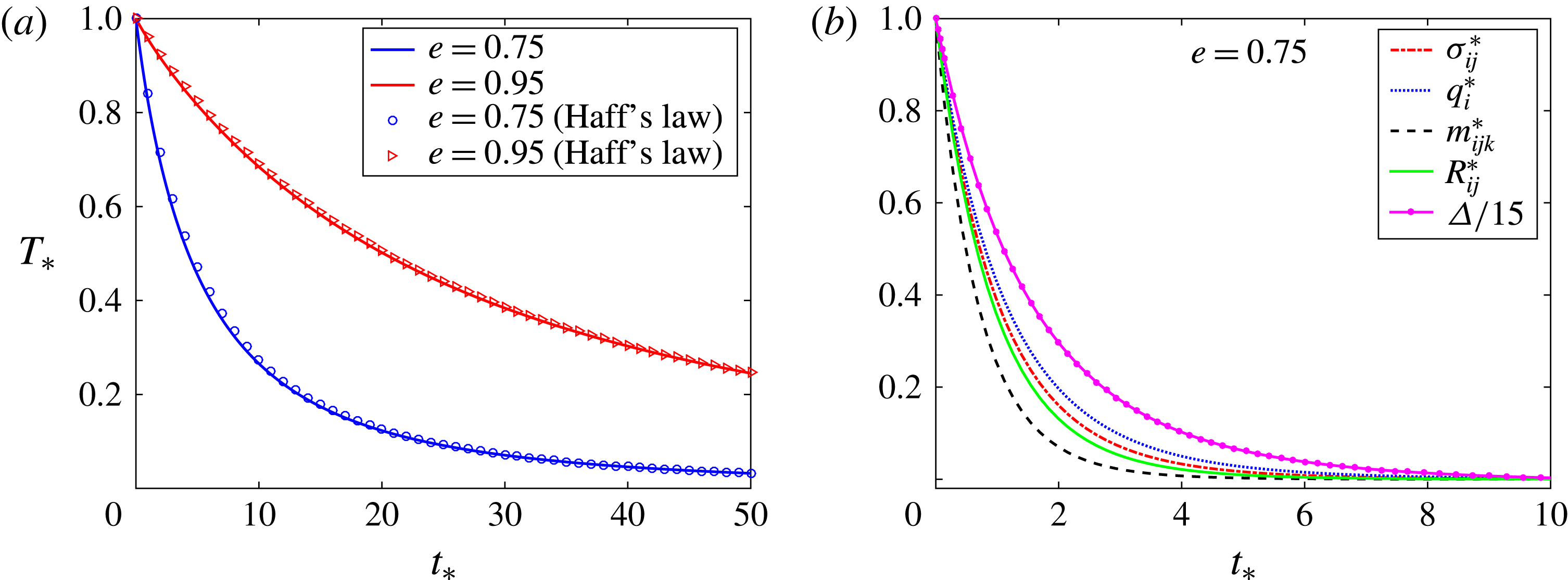
Relaxation of various moments in the HCS. (a) Relaxation of the granular temperature
 $T_{\ast }$
; the lines depict solutions obtained by solving system (4.11)–(4.18) (without the underlined term in (4.18)) while the symbols delineate Haff’s law (4.22); the blue and red colours correspond to the coefficients of restitution
 $e=0.75$
and
 $e=0.95$
respectively. (b) Relaxation of the other moments –
 $\unicode[STIX]{x1D70E}_{ij}^{\ast }$
,
 $q_{i}^{\ast }$
,
 $m_{ijk}^{\ast }$
,
 $R_{ij}^{\ast }$
and
 $(\unicode[STIX]{x1D6E5}/15)$
– for a coefficient of restitution
 $e=0.75$
. The initial conditions are taken as
 $n_{\ast }(0)=T_{\ast }(0)=\unicode[STIX]{x1D70E}_{ij}^{\ast }(0)=q_{i}^{\ast }(0)=m_{ijk}^{\ast }(0)=R_{ij}^{\ast }(0)=1$
,
 $v_{i}^{\ast }(0)=0$
and
 $\unicode[STIX]{x1D6E5}(0)=15$
.

4.2 Relaxation of moments in the HCS
It is clear from (4.11) and (4.12) that the number density
 $n_{\ast }$
remains constant while the macroscopic velocity
 $v_{i}^{\ast }$
remains zero (since there is no macroscopic velocity in the initial state) during the homogeneous cooling. Furthermore, equations (4.14)–(4.18) are coupled and therefore need to be solved numerically for further analysis. It may also be noticed from the structure of (4.15) and (4.16) that vanishing initial conditions on
 $q_{i}^{\ast }$
and
 $m_{ijk}^{\ast }$
will result in a vanishing solution for these quantities. Similarly, vanishing initial conditions on both
 $\unicode[STIX]{x1D70E}_{ij}^{\ast }$
and
 $R_{ij}^{\ast }$
will also result in a zero solution for them. However, due to the coupling on the right-hand sides of (4.14) and (4.17), a non-vanishing initial condition on any one of them will trigger a non-vanishing solution for both of them. On the contrary, a vanishing initial condition on
 $\unicode[STIX]{x1D6E5}$
results in a non-vanishing solution for it for all values of the coefficient of restitution except for
 $e=1$
and
 $e=1/\sqrt{2}$
. In the following analysis, we take the initial conditions as
 $n_{\ast }(0)=T_{\ast }(0)=\unicode[STIX]{x1D70E}_{ij}^{\ast }(0)=q_{i}^{\ast }(0)=m_{ijk}^{\ast }(0)=R_{ij}^{\ast }(0)=1$
,
 $v_{i}^{\ast }(0)=0$
and
 $\unicode[STIX]{x1D6E5}(0)=15$
.
Figure 1 illustrates the numerical solution for the (dimensionless) granular temperature and other higher-order moments obtained by solving the system (4.11)–(4.18) (without the underlined term in (4.18)) along with the aforementioned initial conditions. The solutions for the number density and velocity are not shown since they are just constants. Figure 1(a) exhibits the granular temperature for two values of the coefficient of restitution,
 $e=0.75$
(in blue colour) and
 $e=0.95$
(in red colour). The solid lines depict the numerical solution for the granular temperature obtained by solving the system (4.11)–(4.18) (without the underlined term in (4.18)) along with the aforementioned initial conditions, while the symbols denote the corresponding granular temperature computed via Haff’s law (4.22). Clearly, the numerical results (denoted by solid lines) are in good agreement with those obtained via Haff’s law (denoted by symbols). Moreover, it is also clear that the granular temperature relaxes faster on decreasing the coefficient of restitution. This is due to the fact that more inelastic particles dissipate more energy during the collision in comparison to the less inelastic ones, resulting in the faster decay of the granular temperature for the former in comparison with the latter. The relaxation of the other moments –
 $\unicode[STIX]{x1D70E}_{ij}^{\ast }$
,
 $q_{i}^{\ast }$
,
 $m_{ijk}^{\ast }$
,
 $R_{ij}^{\ast }$
and
 $(\unicode[STIX]{x1D6E5}/15)$
– with time
 $t_{\ast }$
for
 $e=0.75$
is displayed in figure 1(b). It turns out that all of these moments decay with time much faster than the granular temperature. Among them,
 $m_{ijk}^{\ast }$
decays with time
 $t_{\ast }$
faster than any other moment, followed by
 $R_{ij}^{\ast }$
,
 $\unicode[STIX]{x1D70E}_{ij}^{\ast }$
,
 $q_{i}^{\ast }$
and
 $\unicode[STIX]{x1D6E5}$
(in order of fast to slow). That the stress (dashed red line) decays faster than the heat flux (dotted blue line) which decays faster than
 $\unicode[STIX]{x1D6E5}/15$
(magenta line with symbols) is in agreement with the findings of Kremer & Marques Jr (Reference Kremer and Marques2011).
4.3 Effect of nonlinear terms of the dimensionless scalar moment (
$\unicode[STIX]{x1D6E5}$
) on Haff’s law

In § 4.1, we obtained Haff’s law by dropping all the nonlinear terms of the non-equilibrium moments (
 $\unicode[STIX]{x1D70E}_{ij}^{\ast }$
,
 $q_{i}^{\ast }$
,
 $m_{ijk}^{\ast }$
,
 $R_{ij}^{\ast }$
,
 $\unicode[STIX]{x1D6E5}$
) in (4.13) and (4.18). In this subsection, we shall investigate the effect of nonlinear terms of the (dimensionless) scalar moment (
 $\unicode[STIX]{x1D6E5}$
) on Haff’s law in detail.
4.3.1 Case 1: effect of the
$\unicode[STIX]{x1D6E5}^{2}$
term present in (4.18)

The constant
 $\unicode[STIX]{x1D6FC}$
in the characteristic time scale
 $\unicode[STIX]{x1D70F}_{0}$
for the temperature decay via Haff’s law (4.22) was obtained by discarding the
 $\unicode[STIX]{x1D6E5}^{2}$
term in (4.18). We now consider (4.18) without dropping any term. Equation (4.18) has two equilibrium points for
 $e\neq 1$
. Nevertheless, a simple stability analysis of these equilibrium points (see chap. 2 of Strogatz Reference Strogatz1994) shows that only one equilibrium point is stable whereas the other one is unstable. In the limiting case of
 $e\rightarrow 1$
, the stable equilibrium point tends to zero while the unstable equilibrium point tends to infinity. This makes sense as (4.18) in the case of
 $e=1$
has only one equilibrium point (which is zero). Furthermore, in the limiting case of
 $e\rightarrow 1$
, the stable equilibrium point leads to an infinite relaxation time
 $\unicode[STIX]{x1D70F}_{0}$
, which is meaningful for monatomic gases (i.e. for
 $e=1$
). However, the unstable equilibrium point in this limit leads to a finite relaxation time, which is meaningless. For these reasons, we shall neglect the unstable equilibrium point.
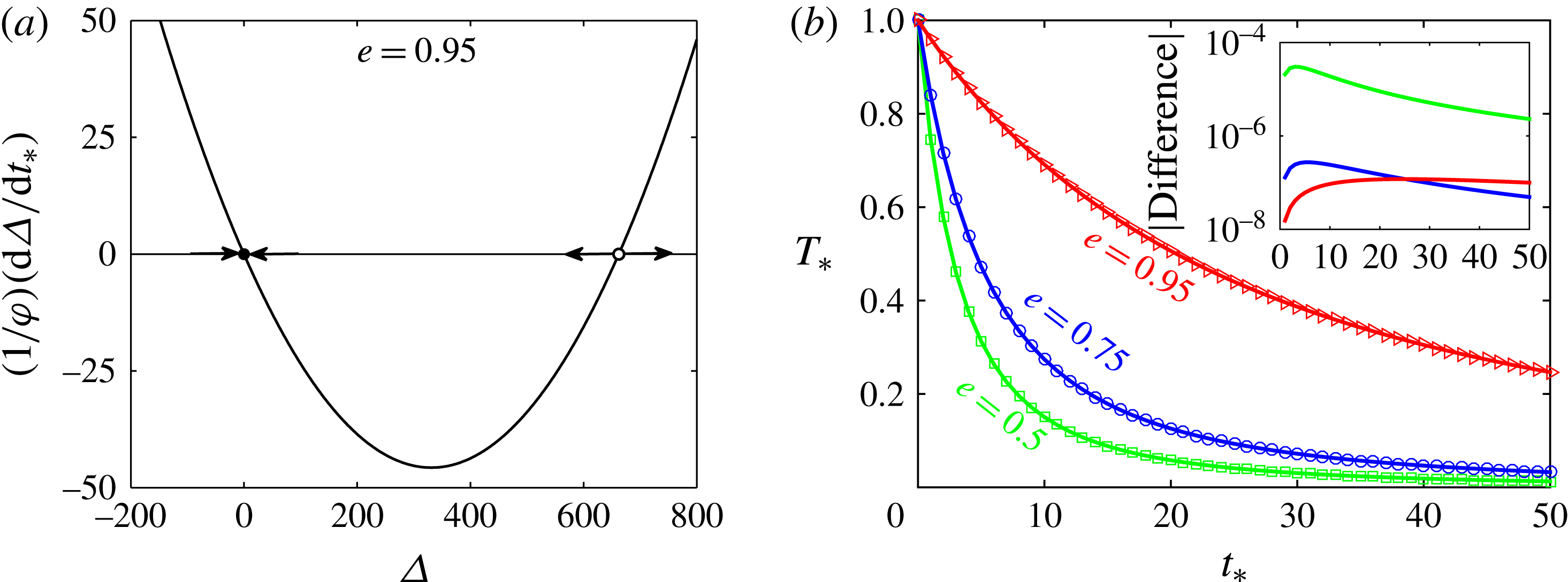
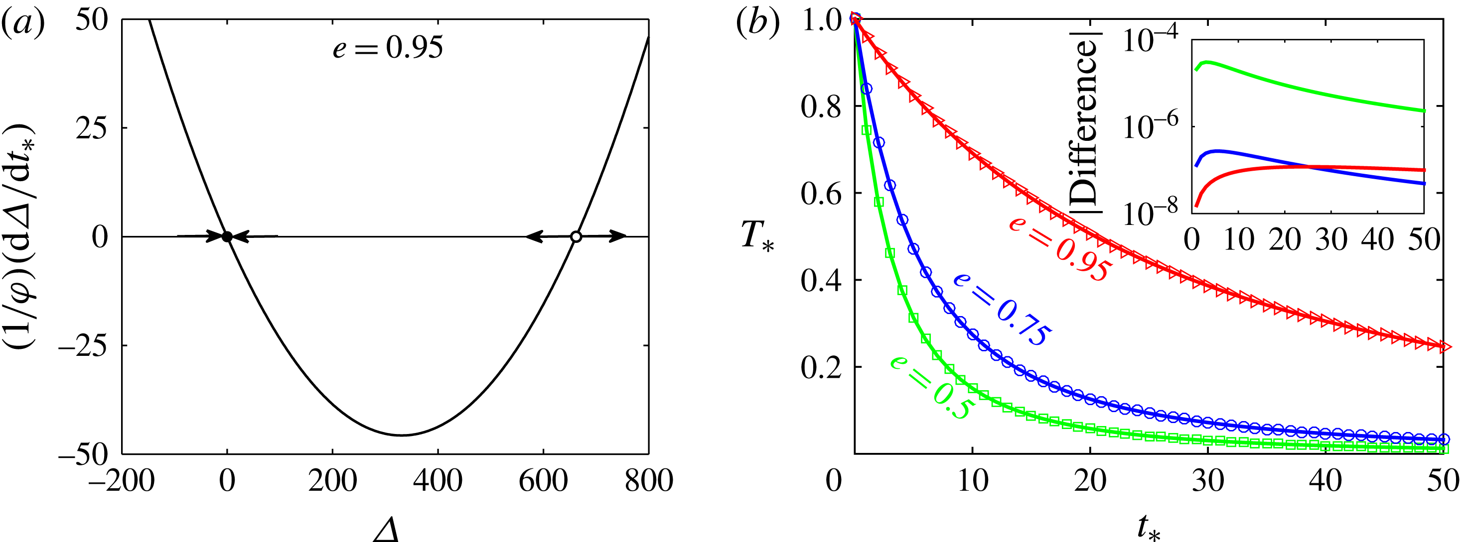
Figure 2(a) portrays the stable (black filled circle) and unstable (white filled circle) equilibrium points for
 $e=0.95$
on a phase portrait. We consider only the stable equilibrium point (black filled circle) and neglect the unstable equilibrium point (white filled circle). The main panel of figure 2(b) illustrates the temperature decay via Haff’s law (4.22) with the inverse time scale (4.23) for three values of the coefficient of restitution,
 $e=0.5,0.75,0.95$
, shown by green, blue and red colours respectively. The solid lines depict Haff’s law when the constant
 $\unicode[STIX]{x1D6FC}$
in (4.23) is taken as the stable equilibrium point of (4.18), while the symbols show that when
 $\unicode[STIX]{x1D6FC}$
is taken as the single equilibrium point (4.24a
) (i.e. in the linear case). In the inset of figure 2(b), we also plot the corresponding absolute difference between the temperature values obtained in the two cases. It turns out that the difference is many orders of magnitude smaller than the original temperature values. Moreover, the difference is even smaller for large values of the coefficient of restitution. Thus, we conclude that the
 $\unicode[STIX]{x1D6E5}^{2}$
term present in (4.18) does not play any significant role on Haff’s law.
Stability of the roots and the temperature decay. (a) Phase portrait showing the stable (black filled circle) and unstable (white filled circle) equilibrium points of (4.18); here,
 $\unicode[STIX]{x1D711}=5\,(1+e)\,n_{\ast }\sqrt{T_{\ast }}/4>0$
(cf. (4.18)), and thus does not play any role in analysing the stability of the equilibrium points. (b) The temperature decay via Haff’s law (4.22), with the inverse time scale (4.23) for
 $e=0.5,0.75,0.95$
, shown by green, blue and red colours respectively; the solid lines represent Haff’s law when the constant
 $\unicode[STIX]{x1D6FC}$
in (4.23) is taken as the stable equilibrium point of (4.18) (marked by the black filled circle in the phase portrait), while the symbols delineate that for
 $\unicode[STIX]{x1D6FC}$
given in (4.24a
); the inset shows the absolute difference between the temperature values in these two cases.
4.3.2 Case 2: effect of
$\unicode[STIX]{x1D6E5}^{2}$
terms present on the right-hand sides of (4.13) and (3.8)

To investigate the effect of nonlinear terms of the scalar moment (i.e.
 $\unicode[STIX]{x1D6E5}^{2}$
terms) on Haff’s law one needs to include
 $\unicode[STIX]{x1D6E5}^{2}$
terms in the production terms of the energy balance equation (2.13) and
 $w$
balance equation (3.8). On including
 $\unicode[STIX]{x1D6E5}^{2}$
terms along with linear terms on the right-hand sides of (2.13) and (3.8), and introducing the scaling (4.10), the new energy and
 $\unicode[STIX]{x1D6E5}$
balance equations in the HCS read
 $$\begin{eqnarray}\frac{\text{d}T_{\ast }}{\text{d}t_{\ast }}=-\frac{5}{12}(1-e^{2})\,n_{\ast }T_{\ast }^{3/2}\left(1+\frac{1}{80}\unicode[STIX]{x1D6E5}+\frac{1}{25600}\unicode[STIX]{x1D6E5}^{2}\right),\end{eqnarray}$$
 $$\begin{eqnarray}\displaystyle \frac{\text{d}\unicode[STIX]{x1D6E5}}{\text{d}t_{\ast }} & = & \displaystyle \frac{5(1+e)}{4}n_{\ast }\sqrt{T_{\ast }}\left[(1-e)(1-2e^{2})-\frac{(81-17e+30e^{2}-30e^{3})}{240}\unicode[STIX]{x1D6E5}\right.\nonumber\\ \displaystyle & & \displaystyle \left.+\,\frac{(1873-2001e+30e^{2}-30e^{3})}{230400}\unicode[STIX]{x1D6E5}^{2}+\frac{(1-e)}{38400}\unicode[STIX]{x1D6E5}^{3}\right].\end{eqnarray}$$
It should be noticed again that although we included the nonlinear terms proportional to
 $\unicode[STIX]{x1D6E5}^{2}$
on the right-hand sides of (2.13) and (3.8), the right-hand side of (4.26) contains
 $\unicode[STIX]{x1D6E5}^{3}$
terms as well. Similarly to above, to obtain Haff’s law from (4.25),
 $\unicode[STIX]{x1D6E5}$
must be a constant, or, in other words, condition (4.21) must be fulfilled. With a constant value of
 $\unicode[STIX]{x1D6E5}$
(
 $=\unicode[STIX]{x1D6FD}$
, let us say), equations (4.11) and (4.25) along with the initial conditions
 $n_{\ast }(0)=T_{\ast }(0)=1$
again yield Haff’s law (4.22). However, the inverse of the dimensionless characteristic time scale in this case reads
 $$\begin{eqnarray}\unicode[STIX]{x1D70F}_{0}^{-1}={\textstyle \frac{5}{24}}(1-e^{2})\left(1+{\textstyle \frac{1}{80}}\unicode[STIX]{x1D6FD}+{\textstyle \frac{1}{25600}}\unicode[STIX]{x1D6FD}^{2}\right).\end{eqnarray}$$
Again, in the light of condition (4.21), the constant
 $\unicode[STIX]{x1D6FD}$
in (4.27) is an equilibrium point of the differential equation (4.26).
Stability of the roots and the temperature decay. (a) Phase portrait showing the stable (black filled circle) and unstable (white filled circles) equilibrium points of (4.26); here,
 $\unicode[STIX]{x1D711}=5\,(1+e)\,n_{\ast }\sqrt{T_{\ast }}/4>0$
(cf. (4.18)), and thus does not play any role in analysing the stability of the equilibrium points. (b) The temperature decay via Haff’s law (4.22) for
 $e=0.5,0.75,0.95$
, shown by green, blue and red colours respectively; the solid lines represent Haff’s law (4.22) with the inverse time scale (4.27) when the constant
 $\unicode[STIX]{x1D6FD}$
in (4.27) is taken as the stable equilibrium point of (4.26) (marked by the black filled circle in the phase portrait), while the symbols delineate Haff’s law (4.22) with the inverse time scale (4.23) and the constant
 $\unicode[STIX]{x1D6FC}$
as given in (4.24a
); the inset shows the absolute difference between the temperature values in these two cases.

Equation (4.26) has three equilibrium points for
 $e\neq 1$
. Again, a simple stability analysis of these equilibrium points (see chap. 2 of Strogatz Reference Strogatz1994) shows that only one equilibrium point is stable whereas the other two are unstable. Figure 3(a) displays the stable (black filled circle) and unstable equilibrium points (white filled circles) for
 $e=0.95$
on a phase portrait. In the limiting case of
 $e\rightarrow 1$
, the stable equilibrium point tends to zero, the left unstable point tends to
 $-480$
and the right unstable equilibrium point tends to infinity. That one equilibrium point of (4.26) in the limiting case of
 $e\rightarrow 1$
tends to infinity makes sense as (4.26) in the case of
 $e=1$
has only two equilibrium points. Furthermore, in the limiting case of
 $e\rightarrow 1$
, the stable equilibrium point and the left unstable equilibrium point lead to an infinite relaxation time
 $\unicode[STIX]{x1D70F}_{0}$
, which is meaningful for monatomic gases (i.e. for
 $e=1$
). However, the right unstable equilibrium point in this limit leads to a vanishing relaxation time, which is meaningless. Therefore, we neglect the right unstable equilibrium point. Although the left unstable equilibrium point leads to a meaningful infinite relaxation time
 $\unicode[STIX]{x1D70F}_{0}$
in the limit
 $e\rightarrow 1$
, its value in the limit
 $e\rightarrow 1$
itself is not meaningful because the equilibrium points are the steady-state solutions of (4.26) and the distribution function for monatomic gases (i.e. for
 $e=1$
) in the steady state is Maxwellian, and, consequently, by definition,
 $w$
(and hence
 $\unicode[STIX]{x1D6E5}$
) must vanish in the limit
 $e\rightarrow 1$
and in the steady state. Therefore, we again consider only the stable equilibrium point (marked by the black filled circle) and neglect the unstable equilibrium points (marked by white filled circles). The main panel of figure 3(b) illustrates the temperature decay via Haff’s law (4.22) for three values of the coefficient of restitution,
 $e=0.5,0.75,0.95$
, shown by green, blue and red colours respectively. The solid lines depict the results obtained with the inverse time scale (4.27) and the constant
 $\unicode[STIX]{x1D6FD}$
in (4.27) as the stable equilibrium point of (4.26) (marked by the black filled circle in the phase portrait), whereas the symbols delineate the corresponding results obtained with the inverse time scale (4.23) and the constant
 $\unicode[STIX]{x1D6FC}$
as given in (4.24a
) (i.e. in the linear case). In the inset of figure 3(b), we also plot the corresponding absolute difference between the temperature values obtained in the two cases. There is practically no difference in the results as the difference is again many orders of magnitude smaller than the original temperature values.
Thus, we conclude that the nonlinear terms of the (dimensionless) scalar moment
 $\unicode[STIX]{x1D6E5}$
do not play any significant role on Haff’s law.
4.4 Effect of a higher-order scalar moment on Haff’s law
In this subsection, we shall analyse the effect of the sixth-order scalar moment
 $u^{3}$
, which is the full trace of the sixth-order moment, on Haff’s law. Nevertheless, for convenience, we introduce a new dimensionless variable
 $\unicode[STIX]{x1D6EF}$
which is related to the sixth-order scalar moment
 $u^{3}$
via
 $$\begin{eqnarray}\unicode[STIX]{x1D6EF}=\frac{m}{\unicode[STIX]{x1D70C}\,\unicode[STIX]{x1D703}^{3}}\int \big(f-f_{M}\big)\big(C^{6}-21\,\unicode[STIX]{x1D703}\,C^{4}\big)\,\text{d}\boldsymbol{c}=\frac{u^{3}}{\unicode[STIX]{x1D70C}\,\unicode[STIX]{x1D703}^{3}}-21\,\unicode[STIX]{x1D6E5}-105,\end{eqnarray}$$
so that
 $\unicode[STIX]{x1D6EF}$
vanishes if it is computed with
 $f$
as either Maxwellian or G13 or G26 distribution function.
We now include the governing equation for the moment
 $\unicode[STIX]{x1D6EF}$
in our existing 26-moment system ((2.11)–(2.13) and (3.4)–(3.8)) and close this system with the Grad distribution function (which we shall term as the G27 distribution function),
 $$\begin{eqnarray}\displaystyle f_{|G27} & = & \displaystyle f_{M}\left[1+\frac{1}{2}\frac{\unicode[STIX]{x1D70E}_{ij}}{\unicode[STIX]{x1D70C}\,\unicode[STIX]{x1D703}^{2}}C_{i}C_{j}+\frac{1}{5}\frac{q_{i}}{\unicode[STIX]{x1D70C}\,\unicode[STIX]{x1D703}^{2}}C_{i}\left(\frac{C^{2}}{\unicode[STIX]{x1D703}}-5\right)+\frac{1}{6}\frac{m_{ijk}}{\unicode[STIX]{x1D70C}\,\unicode[STIX]{x1D703}^{3}}C_{i}C_{j}C_{k}\right.\nonumber\\ \displaystyle & & \displaystyle \left.+\,\frac{1}{28}\frac{R_{ij}}{\unicode[STIX]{x1D70C}\,\unicode[STIX]{x1D703}^{3}}C_{i}C_{j}\left(\frac{C^{2}}{\unicode[STIX]{x1D703}}-7\right)+\frac{1}{8}\unicode[STIX]{x1D6E5}\left(1-\frac{2}{3}\frac{C^{2}}{\unicode[STIX]{x1D703}}+\frac{1}{15}\frac{C^{4}}{\unicode[STIX]{x1D703}^{2}}\right)\right.\nonumber\\ \displaystyle & & \displaystyle \left.-\,\frac{1}{48}\unicode[STIX]{x1D6EF}\left(1-\frac{C^{2}}{\unicode[STIX]{x1D703}}+\frac{1}{5}\frac{C^{4}}{\unicode[STIX]{x1D703}^{2}}-\frac{1}{105}\frac{C^{6}}{\unicode[STIX]{x1D703}^{3}}\right)\right].\end{eqnarray}$$
We shall refer to the system of these 27-moment equations closed with the G27 distribution function as the system of G27 equations.
For our purposes, it is not necessary to derive the full G27 equations, but we do need the production terms for the energy,
 $\unicode[STIX]{x1D6E5}$
and
 $\unicode[STIX]{x1D6EF}$
balance equations. All of the production terms associated with the G27 equations are given in appendix A. It should be noted that the production terms for the
 $\unicode[STIX]{x1D6E5}$
and
 $\unicode[STIX]{x1D6EF}$
balance equations are given by
 $$\begin{eqnarray}\frac{1}{\unicode[STIX]{x1D70C}\unicode[STIX]{x1D703}^{2}}{\mathcal{P}}^{2}-\frac{2}{3}\frac{(\unicode[STIX]{x1D6E5}+15)}{\unicode[STIX]{x1D70C}\unicode[STIX]{x1D703}}{\mathcal{P}}^{1}\quad \text{and}\quad \frac{1}{\unicode[STIX]{x1D70C}\unicode[STIX]{x1D703}^{3}}{\mathcal{P}}^{3}-\frac{21}{\unicode[STIX]{x1D70C}\,\unicode[STIX]{x1D703}^{2}}{\mathcal{P}}^{2}-\frac{(\unicode[STIX]{x1D6EF}-7\unicode[STIX]{x1D6E5}-105)}{\unicode[STIX]{x1D70C}\unicode[STIX]{x1D703}}{\mathcal{P}}^{1}\end{eqnarray}$$
respectively. In the HCS, the dimensionless energy,
 $\unicode[STIX]{x1D6E5}$
and
 $\unicode[STIX]{x1D6EF}$
balance equations from the system of G27 equations – on employing (4.10) and discarding all the nonlinear terms of the non-equilibrium scalar, vector or tensor moments – read
 $$\begin{eqnarray}\frac{\text{d}T_{\ast }}{\text{d}t_{\ast }}=-\frac{5}{12}(1-e^{2})\,n_{\ast }T_{\ast }^{3/2}\left(1+\frac{1}{80}\unicode[STIX]{x1D6E5}-\frac{1}{6720}\unicode[STIX]{x1D6EF}\right),\end{eqnarray}$$
 $$\begin{eqnarray}\displaystyle \frac{\text{d}\unicode[STIX]{x1D6E5}}{\text{d}t_{\ast }} & = & \displaystyle \frac{5}{4}(1+e)\,n_{\ast }\sqrt{T_{\ast }}\bigg[(1-e)(1-2e^{2})-\frac{(81-17e+30e^{2}-30e^{3})}{240}\unicode[STIX]{x1D6E5}\nonumber\\ \displaystyle & & \displaystyle -\,\frac{(191-127e+10e^{2}-10e^{3})}{6720}\unicode[STIX]{x1D6EF}\bigg],\end{eqnarray}$$
 $$\begin{eqnarray}\displaystyle \frac{\text{d}\unicode[STIX]{x1D6EF}}{\text{d}t_{\ast }} & = & \displaystyle -\frac{15}{16}(1+e)\,n_{\ast }\sqrt{T_{\ast }}\bigg[(1-e)(3-12e^{2}+8e^{4})\nonumber\\ \displaystyle & & \displaystyle -\,\frac{(1111-727e-2012e^{2}+1500e^{3}-280e^{4}+280e^{5})}{240}\unicode[STIX]{x1D6E5}\nonumber\\ \displaystyle & & \displaystyle +\,\frac{(2673-241e+5196e^{2}-3660e^{3}+280e^{4}-280e^{5})}{6720}\unicode[STIX]{x1D6EF}\bigg].\end{eqnarray}$$
Clearly, to obtain Haff’s law from (4.31),
 $\unicode[STIX]{x1D6E5}$
and
 $\unicode[STIX]{x1D6EF}$
must be constants, or, in other words, the conditions
 $$\begin{eqnarray}\frac{\text{d}\unicode[STIX]{x1D6E5}}{\text{d}t_{\ast }}=\frac{\text{d}\unicode[STIX]{x1D6EF}}{\text{d}t_{\ast }}=0\end{eqnarray}$$
must be fulfilled. With constant values of
 $\unicode[STIX]{x1D6E5}$
(
 $=\unicode[STIX]{x1D718}_{1}$
, let us say) and
 $\unicode[STIX]{x1D6EF}$
(
 $=\unicode[STIX]{x1D718}_{2}$
, let us say), equations (4.11) and (4.31) along with the initial conditions
 $n_{\ast }(0)=T_{\ast }(0)=1$
again yield Haff’s law (4.22). However, the inverse of the dimensionless characteristic time scale now reads as
 $$\begin{eqnarray}\unicode[STIX]{x1D70F}_{0}^{-1}={\textstyle \frac{5}{24}}(1-e^{2})\left(1+{\textstyle \frac{1}{80}}\unicode[STIX]{x1D718}_{1}-{\textstyle \frac{1}{6720}}\unicode[STIX]{x1D718}_{2}\right).\end{eqnarray}$$
In the light of conditions (4.34), the constants (
 $\unicode[STIX]{x1D718}_{1},\unicode[STIX]{x1D718}_{2}$
) in (4.35) are the equilibrium points (
 $\unicode[STIX]{x1D6E5}_{eq},\unicode[STIX]{x1D6EF}_{eq}$
) of the system of two first-order ordinary differential equations (4.32) and (4.33) (Strogatz Reference Strogatz1994). The system of equations (4.32) and (4.33) has a unique equilibrium point. Figure 4 illustrates the temperature decay via Haff’s law (4.22) for three values of the coefficient of restitution,
 $e=0.5,0.75,0.95$
, shown by green, blue and red colours respectively. The solid lines depict the results obtained with the inverse time scale (4.35) and the constants
 $(\unicode[STIX]{x1D718}_{1},\unicode[STIX]{x1D718}_{2})$
in (4.35) as the unique equilibrium point of (4.32) and (4.33) whereas the symbols delineate the corresponding results obtained with the inverse time scale (4.23) and the constant
 $\unicode[STIX]{x1D6FC}$
as given in (4.24a
). In the inset of figure 4(b), we also plot the corresponding absolute difference between the temperature values obtained in the two cases. Again, there is practically no difference in the results as the differences are many orders of magnitude smaller than the original temperature values.
Temperature decay via Haff’s law (4.22) for
 $e=0.5,0.75,0.95$
, shown by green, blue and red colours respectively; the solid lines depict the results obtained with the inverse time scale (4.35) and the constants
 $(\unicode[STIX]{x1D718}_{1},\unicode[STIX]{x1D718}_{2})$
in (4.35) as the unique equilibrium point of (4.32) and (4.33), whereas the symbols show Haff’s law (4.22) with the inverse time scale (4.23) and the constant
 $\unicode[STIX]{x1D6FC}$
given in (4.24a
); the inset shows the absolute difference between the temperature values in these two cases.

Furthermore, in view of § 4.3, it is expected that the nonlinear terms of the scalar moments in (4.31)–(4.33) would also have only a negligible effect on Haff’s law. Thus, it is concluded empirically that the nonlinear terms of the non-equilibrium scalar moments as well as the higher-order scalar moments do not have any significant effect on Haff’s law. Therefore, it suffices to consider only those moment systems that consist of the fourth-order scalar moment (
 $\unicode[STIX]{x1D6E5}$
), i.e. to consider a 14- or 26-moment system. Moreover, in the production terms of these moment systems, it is sufficient to retain only those nonlinear terms that are products of
 $\unicode[STIX]{x1D6E5}$
and a vector or a tensor. For this reason, equations (4.1)–(4.8) without the underlined term in (4.8) will be referred to as the G26 equations henceforth.
5 Constitutive relations for the stress and heat flux: Navier–Stokes and Fourier laws
The mass, momentum and energy balance equations (2.11)–(2.13) are not closed since they contain the stress (
 $\unicode[STIX]{x1D70E}_{ij}$
), heat flux (
 $q_{i}$
) and cooling rate (
 $\unicode[STIX]{x1D701}$
) as additional unknowns. One of the main goals in the kinetic theory for granular gases is to derive the constitutive relations for these unknowns in order to close the system of mass, momentum and energy balance equations. To the linear approximation in the spatial gradients, these constitutive relations read (see, e.g., Jenkins & Richman Reference Jenkins and Richman1985a
,Reference Jenkins and Richman
b
; Garzó & Dufty Reference Garzó and Dufty1999; Garzó Reference Garzó2013)
 $$\begin{eqnarray}\displaystyle \unicode[STIX]{x1D70E}_{ij}=-2\unicode[STIX]{x1D702}\frac{\unicode[STIX]{x2202}v_{\langle \!i}}{\unicode[STIX]{x2202}x_{j\,\!\rangle }},\quad q_{i}=-\unicode[STIX]{x1D705}\frac{\unicode[STIX]{x2202}T}{\unicode[STIX]{x2202}x_{i}}-\unicode[STIX]{x1D706}\frac{\unicode[STIX]{x2202}n}{\unicode[STIX]{x2202}x_{i}}\quad \text{and}\quad \unicode[STIX]{x1D701}=\unicode[STIX]{x1D701}_{0}+\unicode[STIX]{x1D701}_{1}\frac{\unicode[STIX]{x2202}v_{i}}{\unicode[STIX]{x2202}x_{i}}. & & \displaystyle\end{eqnarray}$$
Equations (5.1a
) and (5.1b
) are the Navier–Stokes law and Fourier law respectively. The coefficients
 $\unicode[STIX]{x1D701}_{0}$
and
 $\unicode[STIX]{x1D701}_{1}$
in (5.1c
) are the zeroth- and first-order contributions respectively to the cooling rate. The transport coefficients
 $\unicode[STIX]{x1D702}$
,
 $\unicode[STIX]{x1D705}$
are referred to as the shear viscosity and thermal conductivity respectively, and the transport coefficient
 $\unicode[STIX]{x1D706}$
is a special coefficient for granular gases which vanishes identically for elastic gases. Typically, these transport coefficients are obtained by a formal CE expansion on the Boltzmann equation (see, e.g., Brey et al.
Reference Brey, Dufty, Kim and Santos1998a
; Sela & Goldhirsch Reference Sela and Goldhirsch1998; Gupta Reference Gupta2011); nevertheless, some authors have also computed them via computer-aided kinetic theory (Noskowicz et al.
Reference Noskowicz, Bar-Lev, Serero and Goldhirsch2007) and via Grad’s method of moments (see, e.g., Jenkins & Richman Reference Jenkins and Richman1985a
; Kremer & Marques Jr Reference Kremer and Marques2011; Garzó Reference Garzó2013). Although Grad’s method of moments does not restrict the coefficient of restitution to close to
 $1$
, the G13 theory of Jenkins & Richman (Reference Jenkins and Richman1985a
) and the Maxwellian iteration procedure on the G14 equations of Kremer & Marques Jr (Reference Kremer and Marques2011) neglect the effect of cooling rate on the transport coefficients. On the other hand, the work of Garzó (Reference Garzó2013) incorporates the effect of the cooling rate on the transport coefficients, and, consequently, the transport coefficients obtained in this work are in good agreement with those obtained via the classical CE expansion. In this section, we shall determine these transport coefficients through the G26 equations ((4.1)–(4.8) without the underlined term in (4.8)). To this end, we shall follow the approach of Garzó (Reference Garzó2013) so that the effect of the cooling rate on the transport coefficients is incorporated.
We are interested in the linear approximation in the spatial gradients. To this end, let us first analyse the zeroth-order contributions in the spatial gradients.
5.1 Zeroth-order contributions in the spatial gradients
To zeroth order in the spatial gradients, the
 $\unicode[STIX]{x1D6E5}$
balance equation (4.8) yields
 $$\begin{eqnarray}\unicode[STIX]{x1D6E5}=15a_{2}.\end{eqnarray}$$
Consequently, to zeroth order in the spatial gradients, the mass, momentum and energy balance equations (4.1)–(4.3) reduce to
 $$\begin{eqnarray}\frac{\unicode[STIX]{x2202}n}{\unicode[STIX]{x2202}t}=0,\quad \frac{\unicode[STIX]{x2202}v_{i}}{\unicode[STIX]{x2202}t}=0\quad \text{and}\quad \frac{\unicode[STIX]{x2202}T}{\unicode[STIX]{x2202}t}=-\unicode[STIX]{x1D701}_{0}T,\end{eqnarray}$$
with
 $$\begin{eqnarray}\unicode[STIX]{x1D701}_{0}=\unicode[STIX]{x1D708}\unicode[STIX]{x1D701}_{0}^{\ast }\quad \text{and}\quad \unicode[STIX]{x1D701}_{0}^{\ast }=\frac{5}{12}(1-e^{2})\left(1+\frac{3\,a_{2}}{16}\right),\end{eqnarray}$$
while the balance equations for the higher moments ((4.4)–(4.7)) simplify to
 $$\begin{eqnarray}-\unicode[STIX]{x1D708}_{\unicode[STIX]{x1D70E}}^{\ast }\unicode[STIX]{x1D70E}_{ij}-\unicode[STIX]{x1D708}_{\unicode[STIX]{x1D70E}R}^{\ast }\frac{R_{ij}}{\unicode[STIX]{x1D703}}=0,\quad q_{i}=0,\quad m_{ijk}=0,\quad -\unicode[STIX]{x1D708}_{R}^{\ast }R_{ij}+\unicode[STIX]{x1D708}_{R\unicode[STIX]{x1D70E}}^{\ast }\unicode[STIX]{x1D703}\unicode[STIX]{x1D70E}_{ij}=0\end{eqnarray}$$
respectively, with
 $$\begin{eqnarray}\left.\begin{array}{@{}rcl@{}}\displaystyle \unicode[STIX]{x1D708}_{\unicode[STIX]{x1D70E}}^{\ast }\ & =\ & \displaystyle \frac{(1+e)(3-e)}{4}\left(1-\frac{a_{2}}{32}\right),\\ \displaystyle \unicode[STIX]{x1D708}_{\unicode[STIX]{x1D70E}R}^{\ast }\ & =\ & \displaystyle \frac{(1+e)(3-e)}{112}\left(1+\frac{3\,a_{2}}{32}\right),\\ \displaystyle \unicode[STIX]{x1D708}_{R}^{\ast }\ & =\ & \displaystyle \frac{(1+e)}{336}\left[(436-267e+66e^{2}-30e^{3})-\frac{(52-27e+66e^{2}-30e^{3})\,a_{2}}{32}\right],\\ \displaystyle \unicode[STIX]{x1D708}_{R\unicode[STIX]{x1D70E}}^{\ast }\ & =\ & \displaystyle \frac{(1+e)}{12}\left[(11-2e-22e^{2}+10e^{3})+\frac{(202-207e-66e^{2}+30e^{3})\,a_{2}}{32}\right].\end{array}\right\}\end{eqnarray}$$
Equations (5.5a,d ) imply that
 $$\begin{eqnarray}\unicode[STIX]{x1D70E}_{ij}=R_{ij}=0.\end{eqnarray}$$
Thus, to zeroth order in the spatial gradients,
 $\unicode[STIX]{x1D70E}_{ij}$
,
 $q_{i}$
,
 $m_{ijk}$
and
 $R_{ij}$
are zero while
 $\unicode[STIX]{x1D6E5}=15a_{2}$
. This means that all of the non-equilibrium vectorial and tensorial moments are at least of linear order in the spatial gradients.
5.2 First-order contributions in the spatial gradients
We now investigate the moments up to first order in the spatial gradients, which will lead to the desired Navier–Stokes and Fourier laws.
To first order in the spatial gradients, the mass, momentum and energy balance equations (4.1)–(4.3) yield
 $$\begin{eqnarray}\displaystyle & \displaystyle \frac{\unicode[STIX]{x2202}n}{\unicode[STIX]{x2202}t}=-v_{i}\frac{\unicode[STIX]{x2202}n}{\unicode[STIX]{x2202}x_{i}}-n\frac{\unicode[STIX]{x2202}v_{i}}{\unicode[STIX]{x2202}x_{i}}, & \displaystyle\end{eqnarray}$$
 $$\begin{eqnarray}\displaystyle & \displaystyle \frac{\unicode[STIX]{x2202}v_{i}}{\unicode[STIX]{x2202}t}=-v_{j}\frac{\unicode[STIX]{x2202}v_{i}}{\unicode[STIX]{x2202}x_{j}}-\frac{1}{mn}\frac{\unicode[STIX]{x2202}(nT)}{\unicode[STIX]{x2202}x_{i}}, & \displaystyle\end{eqnarray}$$
 $$\begin{eqnarray}\displaystyle & \displaystyle \frac{\unicode[STIX]{x2202}T}{\unicode[STIX]{x2202}t}=-v_{i}\frac{\unicode[STIX]{x2202}T}{\unicode[STIX]{x2202}x_{i}}-\frac{2}{3}T\frac{\unicode[STIX]{x2202}v_{i}}{\unicode[STIX]{x2202}x_{i}}-\unicode[STIX]{x1D701}T, & \displaystyle\end{eqnarray}$$
where
 $\unicode[STIX]{x1D701}$
needs to be considered up to linear order in the spatial gradients. Furthermore, the stress and heat flux balance equations ((4.4) and (4.5)), to first order in the spatial gradients, reduce to
 $$\begin{eqnarray}\displaystyle & \displaystyle \frac{\unicode[STIX]{x2202}\unicode[STIX]{x1D70E}_{ij}}{\unicode[STIX]{x2202}t}+2\unicode[STIX]{x1D70C}\unicode[STIX]{x1D703}\frac{\unicode[STIX]{x2202}v_{\langle \!i}}{\unicode[STIX]{x2202}x_{j\,\!\rangle }}=-\unicode[STIX]{x1D708}\left[\unicode[STIX]{x1D708}_{\unicode[STIX]{x1D70E}}^{\ast }\,\unicode[STIX]{x1D70E}_{ij}+\unicode[STIX]{x1D708}_{\unicode[STIX]{x1D70E}R}^{\ast }\frac{R_{ij}}{\unicode[STIX]{x1D703}}\right], & \displaystyle\end{eqnarray}$$
 $$\begin{eqnarray}\displaystyle & \displaystyle \frac{\unicode[STIX]{x2202}q_{i}}{\unicode[STIX]{x2202}t}+\frac{5}{2}a_{2}\left(\unicode[STIX]{x1D703}^{2}\frac{\unicode[STIX]{x2202}\unicode[STIX]{x1D70C}}{\unicode[STIX]{x2202}x_{i}}+2\unicode[STIX]{x1D70C}\unicode[STIX]{x1D703}\frac{\unicode[STIX]{x2202}\unicode[STIX]{x1D703}}{\unicode[STIX]{x2202}x_{i}}\right)+\frac{5}{2}\unicode[STIX]{x1D70C}\unicode[STIX]{x1D703}\frac{\unicode[STIX]{x2202}\unicode[STIX]{x1D703}}{\unicode[STIX]{x2202}x_{i}}=-\unicode[STIX]{x1D708}\unicode[STIX]{x1D708}_{q}^{\ast }\,q_{i}, & \displaystyle\end{eqnarray}$$
with
 $$\begin{eqnarray}\unicode[STIX]{x1D708}_{q}^{\ast }=\frac{(1+e)}{48}\left[(49-33e)+\frac{(19-3e)a_{2}}{32}\right].\end{eqnarray}$$
It should be noticed that we do not need the balance equations for other moments except (4.7), the one for
 $R_{ij}$
, for first-order approximation. Equation (4.7) is only needed because the contribution of
 $R_{ij}$
is required in (5.11). To first order in the spatial gradients, the
 $R_{ij}$
balance equation (4.7) reduces to
 $$\begin{eqnarray}\frac{\unicode[STIX]{x2202}R_{ij}}{\unicode[STIX]{x2202}t}+14a_{2}\unicode[STIX]{x1D70C}\unicode[STIX]{x1D703}^{2}\frac{\unicode[STIX]{x2202}v_{\langle \!i}}{\unicode[STIX]{x2202}x_{j\,\!\rangle }}=-\unicode[STIX]{x1D708}\big[\unicode[STIX]{x1D708}_{R}^{\ast }\,R_{ij}-\unicode[STIX]{x1D708}_{R\unicode[STIX]{x1D70E}}^{\ast }\unicode[STIX]{x1D703}\unicode[STIX]{x1D70E}_{ij}\big].\end{eqnarray}$$
Here, we ignore the time derivative of
 $R_{ij}$
by assuming that it decreases with time faster than stress and heat flux. With this assumption, equation (5.14) yields
 $$\begin{eqnarray}\frac{R_{ij}}{\unicode[STIX]{x1D703}}=\frac{\unicode[STIX]{x1D708}_{R\unicode[STIX]{x1D70E}}^{\ast }}{\unicode[STIX]{x1D708}_{R}^{\ast }}\unicode[STIX]{x1D70E}_{ij}-\frac{14a_{2}\unicode[STIX]{x1D70C}\unicode[STIX]{x1D703}}{\unicode[STIX]{x1D708}\,\unicode[STIX]{x1D708}_{R}^{\ast }}\frac{\unicode[STIX]{x2202}v_{\langle \!i}}{\unicode[STIX]{x2202}x_{j\,\!\rangle }}.\end{eqnarray}$$
With (5.15), equation (5.11) becomes
 $$\begin{eqnarray}\frac{\unicode[STIX]{x2202}\unicode[STIX]{x1D70E}_{ij}}{\unicode[STIX]{x2202}t}+\unicode[STIX]{x1D708}\left(\unicode[STIX]{x1D708}_{\unicode[STIX]{x1D70E}}^{\ast }+\frac{\unicode[STIX]{x1D708}_{\unicode[STIX]{x1D70E}R}^{\ast }\,\unicode[STIX]{x1D708}_{R\unicode[STIX]{x1D70E}}^{\ast }}{\unicode[STIX]{x1D708}_{R}^{\ast }}\right)\unicode[STIX]{x1D70E}_{ij}=-2\left(1-7a_{2}\frac{\unicode[STIX]{x1D708}_{\unicode[STIX]{x1D70E}R}^{\ast }}{\unicode[STIX]{x1D708}_{R}^{\ast }}\right)\unicode[STIX]{x1D70C}\unicode[STIX]{x1D703}\frac{\unicode[STIX]{x2202}v_{\langle \!i}}{\unicode[STIX]{x2202}x_{j\,\!\rangle }}.\end{eqnarray}$$
The time derivatives of the stress and heat flux in (5.16) and (5.12) are now calculated as follows. From (5.1a,b ), we have
 $$\begin{eqnarray}\displaystyle \left.\begin{array}{@{}l@{}}\displaystyle \frac{\unicode[STIX]{x2202}\unicode[STIX]{x1D70E}_{ij}}{\unicode[STIX]{x2202}t}=-2\frac{\unicode[STIX]{x2202}v_{\langle \!i}}{\unicode[STIX]{x2202}x_{j\,\!\rangle }}\frac{\unicode[STIX]{x2202}\unicode[STIX]{x1D702}}{\unicode[STIX]{x2202}t}-\text{}\underline{2\unicode[STIX]{x1D702}\frac{\unicode[STIX]{x2202}}{\unicode[STIX]{x2202}x_{j\,\!\rangle }}\frac{\unicode[STIX]{x2202}v_{\langle \!i}}{\unicode[STIX]{x2202}t}},\\ \displaystyle \frac{\unicode[STIX]{x2202}q_{i}}{\unicode[STIX]{x2202}t}=-\frac{\unicode[STIX]{x2202}T}{\unicode[STIX]{x2202}x_{i}}\frac{\unicode[STIX]{x2202}\unicode[STIX]{x1D705}}{\unicode[STIX]{x2202}t}-\unicode[STIX]{x1D705}\underbrace{\frac{\unicode[STIX]{x2202}}{\unicode[STIX]{x2202}x_{i}}\frac{\unicode[STIX]{x2202}T}{\unicode[STIX]{x2202}t}}_{}-\frac{\unicode[STIX]{x2202}n}{\unicode[STIX]{x2202}x_{i}}\frac{\unicode[STIX]{x2202}\unicode[STIX]{x1D706}}{\unicode[STIX]{x2202}t}-\text{}\underline{\unicode[STIX]{x1D706}\frac{\unicode[STIX]{x2202}}{\unicode[STIX]{x2202}x_{i}}\frac{\unicode[STIX]{x2202}n}{\unicode[STIX]{x2202}t}}.\end{array}\right\} & & \displaystyle\end{eqnarray}$$
For first-order approximation in the spatial gradients, the time derivatives on the right-hand sides of (5.17) are required only up to zeroth order in spatial gradients. Hence, by virtue of (5.3), the underlined terms in (5.17) vanish while the underbraced term in (5.17b ) becomes
 $$\begin{eqnarray}\frac{\unicode[STIX]{x2202}}{\unicode[STIX]{x2202}x_{i}}\frac{\unicode[STIX]{x2202}T}{\unicode[STIX]{x2202}t}=-\unicode[STIX]{x1D701}_{0}\frac{\unicode[STIX]{x2202}T}{\unicode[STIX]{x2202}x_{i}}-T\unicode[STIX]{x1D701}_{0}^{\ast }\frac{\unicode[STIX]{x2202}\unicode[STIX]{x1D708}}{\unicode[STIX]{x2202}x_{i}}=-\frac{3}{2}\unicode[STIX]{x1D701}_{0}\frac{\unicode[STIX]{x2202}T}{\unicode[STIX]{x2202}x_{i}}-\unicode[STIX]{x1D701}_{0}\frac{T}{n}\frac{\unicode[STIX]{x2202}n}{\unicode[STIX]{x2202}x_{i}}.\end{eqnarray}$$
By dimensional analysis, it turns out that
 $\unicode[STIX]{x1D702}\propto \sqrt{T}$
,
 $\unicode[STIX]{x1D705}\propto \sqrt{T}$
and
 $\unicode[STIX]{x1D706}\propto T^{3/2}$
. Therefore, to zeroth order in spatial gradients, on using (5.3c
), the time derivatives of the transport coefficients read
 $$\begin{eqnarray}\frac{\unicode[STIX]{x2202}\unicode[STIX]{x1D702}}{\unicode[STIX]{x2202}t}=-\frac{1}{2}\unicode[STIX]{x1D702}\unicode[STIX]{x1D701}_{0},\quad \frac{\unicode[STIX]{x2202}\unicode[STIX]{x1D705}}{\unicode[STIX]{x2202}t}=-\frac{1}{2}\unicode[STIX]{x1D705}\unicode[STIX]{x1D701}_{0}\quad \text{and}\quad \frac{\unicode[STIX]{x2202}\unicode[STIX]{x1D706}}{\unicode[STIX]{x2202}t}=-\frac{3}{2}\unicode[STIX]{x1D706}\unicode[STIX]{x1D701}_{0}.\end{eqnarray}$$
The time derivatives of the stress and heat flux (5.17), on using (5.18) and (5.19), become
 $$\begin{eqnarray}\frac{\unicode[STIX]{x2202}\unicode[STIX]{x1D70E}_{ij}}{\unicode[STIX]{x2202}t}=\unicode[STIX]{x1D702}\unicode[STIX]{x1D701}_{0}\frac{\unicode[STIX]{x2202}v_{\langle \!i}}{\unicode[STIX]{x2202}x_{j\,\!\rangle }}\quad \text{and}\quad \frac{\unicode[STIX]{x2202}q_{i}}{\unicode[STIX]{x2202}t}=2\unicode[STIX]{x1D705}\unicode[STIX]{x1D701}_{0}\frac{\unicode[STIX]{x2202}T}{\unicode[STIX]{x2202}x_{i}}+\left(\unicode[STIX]{x1D705}\frac{T}{n}+\frac{3}{2}\unicode[STIX]{x1D706}\right)\unicode[STIX]{x1D701}_{0}\frac{\unicode[STIX]{x2202}n}{\unicode[STIX]{x2202}x_{i}}.\end{eqnarray}$$
By inserting the time derivatives of the stress and heat flux from (5.20) into (5.16) and (5.12), and comparing the coefficients of the spatial gradient of each hydrodynamic variable, one obtains the transport coefficients in the Navier–Stokes and Fourier laws (5.1a,b ) as
 $$\begin{eqnarray}\unicode[STIX]{x1D702}=\unicode[STIX]{x1D702}_{0}\unicode[STIX]{x1D702}^{\ast },\quad \unicode[STIX]{x1D705}=\unicode[STIX]{x1D705}_{0}\unicode[STIX]{x1D705}^{\ast }\quad \text{and}\quad \unicode[STIX]{x1D706}=\frac{\unicode[STIX]{x1D705}_{0}T}{n}\unicode[STIX]{x1D706}^{\ast },\end{eqnarray}$$
where
 $$\begin{eqnarray}\unicode[STIX]{x1D702}_{0}=\frac{nT}{\unicode[STIX]{x1D708}}=\frac{5}{16\sqrt{\unicode[STIX]{x03C0}}}\frac{\sqrt{mT}}{d^{2}}\quad \text{and}\quad \unicode[STIX]{x1D705}_{0}=\frac{15}{4m}\unicode[STIX]{x1D702}_{0}=\frac{75}{64\sqrt{\unicode[STIX]{x03C0}}}\frac{1}{d^{2}}\sqrt{\frac{T}{m}}\end{eqnarray}$$
are the elastic values (in the first Sonine approximation) of the shear viscosity and thermal conductivity respectively. They are also referred to as the Enskog viscosity and Enskog thermal conductivity respectively (Brilliantov & Pöschel Reference Brilliantov and Pöschel2004). Moreover,
 $\unicode[STIX]{x1D702}^{\ast }$
,
 $\unicode[STIX]{x1D705}^{\ast }$
and
 $\unicode[STIX]{x1D706}^{\ast }$
in (5.21) are the reduced shear viscosity, reduced thermal conductivity and reduced coefficient corresponding to
 $\unicode[STIX]{x1D706}$
respectively. These reduced transport coefficients are given by
 $$\begin{eqnarray}\unicode[STIX]{x1D702}^{\ast }=\frac{1-7a_{2}\displaystyle \frac{\unicode[STIX]{x1D708}_{\unicode[STIX]{x1D70E}R}^{\ast }}{\unicode[STIX]{x1D708}_{R}^{\ast }}}{\displaystyle \unicode[STIX]{x1D708}_{\unicode[STIX]{x1D70E}}^{\ast }+\frac{\unicode[STIX]{x1D708}_{\unicode[STIX]{x1D70E}R}^{\ast }\unicode[STIX]{x1D708}_{R\unicode[STIX]{x1D70E}}^{\ast }}{\unicode[STIX]{x1D708}_{R}^{\ast }}-\frac{1}{2}\unicode[STIX]{x1D701}_{0}^{\ast }},\quad \unicode[STIX]{x1D705}^{\ast }=\frac{2}{3}\left[\frac{1+2a_{2}}{\unicode[STIX]{x1D708}_{q}^{\ast }-2\unicode[STIX]{x1D701}_{0}^{\ast }}\right],\quad \unicode[STIX]{x1D706}^{\ast }=\frac{\unicode[STIX]{x1D705}^{\ast }\unicode[STIX]{x1D701}_{0}^{\ast }+\frac{2}{3}a_{2}}{\unicode[STIX]{x1D708}_{q}^{\ast }-\frac{3}{2}\unicode[STIX]{x1D701}_{0}^{\ast }}.\end{eqnarray}$$
If we take
 $\unicode[STIX]{x1D708}_{\unicode[STIX]{x1D70E}R}^{\ast }=0$
, i.e. if we ignore the contribution of
 $R_{ij}$
, the reduced transport coefficients (5.23) obtained here agree with those obtained via Grad’s method of moments in Garzó (Reference Garzó2013) for dilute granular gases and also with those obtained by first Sonine approximation via the CE expansion in Brey et al. (Reference Brey, Dufty, Kim and Santos1998a
). If we further neglect the cooling effect (i.e.
 $\unicode[STIX]{x1D701}_{0}^{\ast }=0$
) as well, the reduced transport coefficients obtained here concur with those derived in Kremer & Marques Jr (Reference Kremer and Marques2011).
In the elastic case (
 $e=1$
), the reported (exact) value of the reduced shear viscosity
 $\unicode[STIX]{x1D702}^{\ast }$
is
 $1.016034$
, which was obtained by Pekeris & Alterman (Reference Pekeris and Alterman1957) by reducing the Boltzmann equation to an ordinary differential equation of order
 $4$
and subsequently integrating it numerically. Reinecke & Kremer (Reference Reinecke and Kremer1990) obtained almost the same value,
 $\unicode[STIX]{x1D702}^{\ast }\approx 1.016028$
, for the reduced shear viscosity by employing the Maxwell iteration procedure on the Grad moment equations, at fifth order of approximation. The reduced shear viscosity for
 $e=1$
obtained from (5.23a
) is
 $\unicode[STIX]{x1D702}^{\ast }=205/202({\approx}1.014851)$
, which is exactly the same as that obtained at second-order approximation in Reinecke & Kremer (Reference Reinecke and Kremer1990), thanks to the coupling between
 $\unicode[STIX]{x1D70E}_{ij}$
and
 $R_{ij}$
in their balance equations. It should be noted that the first Sonine approximation (Brey et al.
Reference Brey, Dufty, Kim and Santos1998a
), the modified Sonine approximation (Garzó, Santos & Montanero Reference Garzó, Santos and Montanero2007), the G14 theory of Kremer & Marques Jr (Reference Kremer and Marques2011) and the Grad moment theory of Garzó (Reference Garzó2013) all in the elastic case lead to
 $\unicode[STIX]{x1D702}^{\ast }=1$
, which is the value obtained at first-order approximation in Reinecke & Kremer (Reference Reinecke and Kremer1990). Furthermore, the reported value of the reduced thermal conductivity
 $\unicode[STIX]{x1D705}^{\ast }$
in the elastic case is
 $1.025218$
(Pekeris & Alterman Reference Pekeris and Alterman1957). Reinecke & Kremer (Reference Reinecke and Kremer1990) again obtained almost the same value,
 $\unicode[STIX]{x1D705}^{\ast }\approx 1.025197$
, at fifth-order approximation. However, the reduced thermal conductivity obtained here as well as that obtained by all of the four aforementioned approaches is
 $\unicode[STIX]{x1D705}^{\ast }=1$
, which is the value obtained at first-order approximation in Reinecke & Kremer (Reference Reinecke and Kremer1990). The reason for not obtaining an improved value of the reduced thermal conductivity here is that, unlike the right-hand side of the stress balance equation which is coupled with the one trace of the fourth moment (
 $R_{ij}$
), the right-hand side of the heat flux balance equation does not have any coupling with other vectorial or tensorial moments in its considered form.
5.3 Comparison with existing theories and computer simulations
In this subsection, we shall compare the reduced transport coefficients derived here with those obtained by the CE expansion as well as with those obtained through computer simulations.
Figure 5 illustrates the reduced shear viscosity
 $\unicode[STIX]{x1D702}^{\ast }$
while figure 6 illustrates the reduced thermal conductivity
 $\unicode[STIX]{x1D705}^{\ast }$
and reduced coefficient
 $\unicode[STIX]{x1D706}^{\ast }$
for different values of the coefficient of restitution. The solid (black) lines in both the figures represent the results obtained with expressions (5.23) in the present work. The dashed (green) lines are the plots for the reduced transport coefficients derived at the first Sonine approximation through the CE expansion performed on the Boltzmann equation in Brey et al. (Reference Brey, Dufty, Kim and Santos1998a
). As the reduced transport coefficients obtained via Grad’s method of moments in Garzó (Reference Garzó2013) coincide with those in Brey et al. (Reference Brey, Dufty, Kim and Santos1998a
), the dashed (green) lines also display the reduced transport coefficients obtained in Garzó (Reference Garzó2013). The dash-dotted (magenta) lines display the results obtained with the theoretical expressions for the reduced transport coefficients deduced through the modified version of the first Sonine approximation in Garzó et al. (Reference Garzó, Santos and Montanero2007). The squares are the results obtained with the theoretical expressions derived via the so-called computer-aided method devised by Noskowicz et al. (Reference Noskowicz, Bar-Lev, Serero and Goldhirsch2007), while the triangles denote the numerical solution of the Boltzmann equation obtained through Green–Kubo (GK) relations by means of the direct-simulation Monte Carlo (DSMC) method (Bird Reference Bird1994) in Brey et al. (Reference Brey, Ruiz-Montero, Maynar and García de Soria2005). The circles in figure 5 also denote the DSMC simulation results from Montanero, Santos & Garzó (Reference Montanero, Santos and Garzó2005) obtained with another method – by the implementation of an external force that compensates for the collisional cooling. The DSMC simulation data from this method for
 $e=\{0.6,0.7,0.8,0.9,1\}$
were obtained by Montanero et al. (Reference Montanero, Santos and Garzó2005), while those for
 $e=\{0.2,0.3,0.4,0.5\}$
were obtained by Garzó et al. (Reference Garzó, Santos and Montanero2007).
Variation of the reduced shear viscosity
 $\unicode[STIX]{x1D702}^{\ast }$
with the coefficient of restitution
 $e$
. The solid (black) line represents the results obtained in the present work. The dashed (green) and dash-dotted (magenta) lines delineate the first Sonine approximation (Brey et al.
Reference Brey, Dufty, Kim and Santos1998a
) and the modified version of the first Sonine approximation (Garzó et al.
Reference Garzó, Santos and Montanero2007) respectively. The squares are the results from the theoretical expressions obtained via the computer-aided method devised by Noskowicz et al. (Reference Noskowicz, Bar-Lev, Serero and Goldhirsch2007). The other symbols are the DSMC simulation results of Brey et al. (Reference Brey, Ruiz-Montero, Maynar and García de Soria2005) obtained using GK relations (triangles) and of Montanero et al. (Reference Montanero, Santos and Garzó2005) obtained with the implementation of an external force (circles).

Variation of (a) the reduced thermal conductivity
 $\unicode[STIX]{x1D705}^{\ast }$
and (b) the reduced coefficient
 $\unicode[STIX]{x1D706}^{\ast }$
with the coefficient of restitution
 $e$
. The lines and symbols are the same as described in figure 5.

In general, the reduced shear viscosity from the first Sonine approximation (dashed green line) agrees with that from the DSMC simulations using GK relations (triangles). Nevertheless, the results from the DSMC simulations with the implementation of external force (shown by circles) differ from those obtained with the GK relations (shown by triangles), especially for
 $e\lesssim 0.7$
. The difference between the results from the two simulations could be due to velocity correlations in the correlation function present in the GK relation for the shear viscosity (Garzó et al.
Reference Garzó, Santos and Montanero2007). In comparison with the results from the modified version of the first Sonine approximation (dash-dotted magenta line), the present results for the reduced shear viscosity (solid black line) are in better agreement with the DSMC simulations of Garzó et al. (Reference Garzó, Santos and Montanero2007) even for small coefficient of restitutions. Furthermore, the present results for the reduced shear viscosity (solid black line) coincide with those obtained from the computer-aided method devised by Noskowicz et al. (Reference Noskowicz, Bar-Lev, Serero and Goldhirsch2007) (shown by squares) for almost all values of the coefficient of restitution. Nevertheless, in the elastic (
 $e=1$
) case, the theoretical expressions of Noskowicz et al. (Reference Noskowicz, Bar-Lev, Serero and Goldhirsch2007) lead to
 $\unicode[STIX]{x1D702}^{\ast }=1.01205$
, while the DSMC simulations of Garzó et al. (Reference Garzó, Santos and Montanero2007) give
 $\unicode[STIX]{x1D702}^{\ast }\approx 1.016$
. Thus, in the elastic (
 $e=1$
) case,
 $\unicode[STIX]{x1D702}^{\ast }\approx 1.014851$
from the expression (5.23a
) obtained here is much closer to its true value in comparison with that from the theoretical expressions of Noskowicz et al. (Reference Noskowicz, Bar-Lev, Serero and Goldhirsch2007).
The expressions for the reduced transport coefficients corresponding to the heat flux (i.e. for
 $\unicode[STIX]{x1D705}^{\ast }$
and
 $\unicode[STIX]{x1D706}^{\ast }$
) derived here are the same as those obtained via the first Sonine approximation (Brey et al.
Reference Brey, Dufty, Kim and Santos1998a
) and via the Grad moment method of Garzó (Reference Garzó2013) because in the considered linearized form, the right-hand side of the heat flux balance equation (4.5) does not couple with any other vectorial or tensorial moments. Therefore, the curves of the reduced thermal conductivity
 $\unicode[STIX]{x1D705}^{\ast }$
and the reduced coefficient
 $\unicode[STIX]{x1D706}^{\ast }$
in figure 6 from (5.23b,c
) (solid black lines) coincide with those from the first Sonine approximation (Brey et al.
Reference Brey, Dufty, Kim and Santos1998a
) or from the Grad moment method of Garzó (Reference Garzó2013) (dashed green lines). It is clear from figure 6 that the results for
 $\unicode[STIX]{x1D705}^{\ast }$
and
 $\unicode[STIX]{x1D706}^{\ast }$
from the present work, from the first Sonine approximation and from Garzó (Reference Garzó2013) agree with the DSMC simulations as well as with those from the computer-aided method of Noskowicz et al. (Reference Noskowicz, Bar-Lev, Serero and Goldhirsch2007) only for a large coefficient of restitution (
 $e\gtrsim 0.7$
). For
 $e\lesssim 0.7$
, similarly to the first Sonine approximation and the Grad moment method of Garzó (Reference Garzó2013), the present work also overestimates both the transport coefficients.
Motivated by the satisfactory result for the reduced shear viscosity through the G26 equations, it is expected that a suitable coupling on the right-hand side of the heat flux balance equation (4.5) would improve the reduced transport coefficients
 $\unicode[STIX]{x1D705}^{\ast }$
and
 $\unicode[STIX]{x1D706}^{\ast }$
significantly. The first such coupling of the right-hand side of the heat flux balance equation in the semi-linearized setting as considered here will be introduced on including the full trace of the fifth-order moment into the moment system, i.e. one would need to consider the system of 29-moment equations. This is beyond the scope of the present paper and will be considered elsewhere in the future.
Although the modified Sonine approach (Garzó et al.
Reference Garzó, Santos and Montanero2007) is an excellent theoretical approach, the predictions of which for all the transport coefficients (
 $\unicode[STIX]{x1D702}^{\ast }$
,
 $\unicode[STIX]{x1D705}^{\ast }$
and
 $\unicode[STIX]{x1D706}^{\ast }$
) are in very good agreement with the simulation results, the G26 theory slightly improves the results for the reduced shear viscosity coefficient
 $\unicode[STIX]{x1D702}^{\ast }$
. However, the latter could not yield the other two transport coefficients related to the heat flux (
 $\unicode[STIX]{x1D705}^{\ast }$
and
 $\unicode[STIX]{x1D706}^{\ast }$
) correctly for
 $e\lesssim 0.7$
, exactly in the same way as the first Sonine approach (Brey et al.
Reference Brey, Dufty, Kim and Santos1998a
). Here, it is worthwhile to note that while it is an important validity test for moment equations to compute the precise form of the transport coefficients, it is well known that these coefficients have only a little relevance in non-equilibrium situations when a linear relation between fluxes and gradients does not hold anymore. Instead, it has been shown (for elastic gases) that moment equations allow for cross-effects like thermal stresses and non-gradient heat fluxes (Torrilhon Reference Torrilhon2016) that are expected to also have a systematic influence in granular flows. The actual goal of moment equations is not only to match the transport coefficients but also to go beyond these classical theories and provide an enhanced fluid dynamic theory for granular gases. Moreover, our long-term perspective is to establish a complete set of predictive moment equations, somewhat similar to the R13 equations for monatomic gases, for granular flows, which certainly requires the G26 equations or beyond. Thus, this work is the first step towards this long-term goal.
6 Linear stability analysis
In this section, we investigate the stability of the HCS due to small perturbations through various moment theories, in particular the G26 theory (equations (4.1)–(4.8) without the underlined term in (4.8)), developed in the earlier sections. We assume that the amplitudes of these perturbations are sufficiently small so that the linear analysis remains valid.
For the linear stability analysis, we decompose all the field variables into their reference values, i.e. their respective solutions in the HCS, and into perturbations from their respective solutions in the HCS, i.e. we define
 $$\begin{eqnarray}\displaystyle \left.\begin{array}{@{}rcl@{}}\displaystyle n(t,\boldsymbol{x})\ & =\ & \displaystyle n_{0}\big[1+{\tilde{n}}(t,\boldsymbol{x})\big],\\ \displaystyle T(t,\boldsymbol{x})\ & =\ & \displaystyle T_{H}(t)\big[1+\tilde{T}(t,\boldsymbol{x})\big],\\ \displaystyle v_{i}(t,\boldsymbol{x})\ & =\ & \displaystyle v_{H}(t)\tilde{v}_{i}(t,\boldsymbol{x}),\\ \displaystyle \unicode[STIX]{x1D70E}_{ij}(t,\boldsymbol{x})\ & =\ & \displaystyle \unicode[STIX]{x1D70E}_{ij}^{(H)}(t)+n_{0}T_{H}(t)\,\tilde{\unicode[STIX]{x1D70E}}_{ij}(t,\boldsymbol{x}),\\ \displaystyle q_{i}(t,\boldsymbol{x})\ & =\ & \displaystyle q_{i}^{(H)}(t)+n_{0}\,T_{H}(t)v_{H}(t)\tilde{q}_{i}(t,\boldsymbol{x}),\\ \displaystyle m_{ijk}(t,\boldsymbol{x})\ & =\ & \displaystyle m_{ijk}^{(H)}(t)+n_{0}T_{H}(t)v_{H}(t)\tilde{m}_{ijk}(t,\boldsymbol{x}),\\ \displaystyle R_{ij}(t,\boldsymbol{x})\ & =\ & \displaystyle R_{ij}^{(H)}(t)+n_{0}T_{H}(t)v_{H}(t)^{2}\tilde{R}_{ij}(t,\boldsymbol{x}),\\ \displaystyle \unicode[STIX]{x1D6E5}(t,\boldsymbol{x})\ & =\ & \displaystyle \unicode[STIX]{x1D6E5}_{H}+\tilde{\unicode[STIX]{x1D6E5}}(t,\boldsymbol{x}),\end{array}\right\} & & \displaystyle\end{eqnarray}$$
where
 $n_{0}$
is the constant number density and
 $T_{H}(t)$
is the granular temperature in the HCS;
 $\unicode[STIX]{x1D6E5}_{H}$
is the constant solution for
 $\unicode[STIX]{x1D6E5}$
in the HCS;
 $v_{H}(t)=\sqrt{T_{H}(t)/m}$
is a reference speed in the HCS and is proportional to the adiabatic sound speed in the HCS; the reference values (HCS solutions) for all other field variables are denoted by the superscript ‘
 $(H)$
’; the quantities with tildes denote the dimensionless perturbations in the field variables from their respective solutions in the HCS. It should be noted that as the underlined term in (4.8) is discarded, the HCS solution for
 $\unicode[STIX]{x1D6E5}$
is
 $\unicode[STIX]{x1D6E5}_{H}=15\,a_{2}$
.
By inserting the field variables from (6.1) into the G26 equations, and neglecting all the nonlinear terms of the perturbed field variables (denoted with tildes in (6.1)), one obtains the system of linear partial differential equations in (dimensionless) perturbed field variables with time-dependent coefficients, which is given in appendix B. These equations are further simplified by exploiting the fact, concluded in § 4.2, that in the HCS, the non-equilibrium vectorial and tensorial moments –
 $\unicode[STIX]{x1D70E}_{ij}^{(H)}(t)$
,
 $q_{i}^{(H)}(t)$
,
 $m_{ijk}^{(H)}(t)$
,
 $R_{ij}^{(H)}(t)$
– decay faster than the granular temperature
 $T_{H}(t)$
; therefore, we drop the terms containing
 $\unicode[STIX]{x1D70E}_{ij}^{(H)}(t)$
,
 $q_{i}^{(H)}(t)$
,
 $m_{ijk}^{(H)}(t)$
,
 $R_{ij}^{(H)}(t)$
in (B 1)–(B 8). Now, it is possible to convert this system of partial differential equations to a new system of partial differential equations having constant coefficients as follows. We introduce a length scale
 $$\begin{eqnarray}\ell =\frac{v_{H}(t)}{\unicode[STIX]{x1D708}_{H}(t)},\quad \text{where}\quad \unicode[STIX]{x1D708}_{H}(t)=\frac{16}{5}\sqrt{\unicode[STIX]{x03C0}}n_{0}d^{2}\sqrt{\frac{T_{H}(t)}{m}},\end{eqnarray}$$
to make the space variables dimensionless (i.e.
 $\tilde{x}_{i}=x_{i}/\ell$
, where tilde again denotes the dimensionless space variable), and a dimensionless time
 $\tilde{t}$
(see McNamara Reference McNamara1993) such that
 $$\begin{eqnarray}\frac{1}{\unicode[STIX]{x1D708}_{H}(t)}\frac{\unicode[STIX]{x2202}}{\unicode[STIX]{x2202}t}(\cdot )=\frac{\unicode[STIX]{x2202}}{\unicode[STIX]{x2202}\tilde{t}}(\cdot ).\end{eqnarray}$$
This leads to
 $$\begin{eqnarray}\tilde{t}=\unicode[STIX]{x1D708}_{H}(t)\unicode[STIX]{x1D70F}_{1}\left(1+\frac{t}{\unicode[STIX]{x1D70F}_{1}}\right)\ln \left(1+\frac{t}{\unicode[STIX]{x1D70F}_{1}}\right)\approx \unicode[STIX]{x1D708}_{H}(t)t+O(t^{2}),\end{eqnarray}$$
where
 $$\begin{eqnarray}\unicode[STIX]{x1D70F}_{1}^{-1}=\frac{1}{2}\unicode[STIX]{x1D701}_{0}^{\ast }\,\unicode[STIX]{x1D708}_{0},\quad \text{with}\quad \unicode[STIX]{x1D708}_{0}=\frac{16}{5}\sqrt{\unicode[STIX]{x03C0}}\,n_{0}d^{2}\sqrt{\frac{T_{0}}{m}}.\end{eqnarray}$$
With these definitions of dimensionless space and time, system (B 1)–(B 8) now simplifies to
 $$\begin{eqnarray}\displaystyle \frac{\unicode[STIX]{x2202}{\tilde{n}}}{\unicode[STIX]{x2202}\tilde{t}}+\frac{\unicode[STIX]{x2202}\tilde{v}_{i}}{\unicode[STIX]{x2202}\tilde{x}_{i}} & = & \displaystyle 0,\end{eqnarray}$$
 $$\begin{eqnarray}\displaystyle \frac{\unicode[STIX]{x2202}\tilde{v}_{i}}{\unicode[STIX]{x2202}\tilde{t}}+\frac{\unicode[STIX]{x2202}\tilde{\unicode[STIX]{x1D70E}}_{ij}}{\unicode[STIX]{x2202}\tilde{x}_{j}}+\frac{\unicode[STIX]{x2202}{\tilde{n}}}{\unicode[STIX]{x2202}\tilde{x}_{i}}+\frac{\unicode[STIX]{x2202}\tilde{T}}{\unicode[STIX]{x2202}\tilde{x}_{i}}-\frac{1}{2}\unicode[STIX]{x1D709}_{0}\tilde{v}_{i} & = & \displaystyle 0,\end{eqnarray}$$
 $$\begin{eqnarray}\displaystyle \frac{\unicode[STIX]{x2202}\tilde{T}}{\unicode[STIX]{x2202}\tilde{t}}+\frac{2}{3}\left(\frac{\unicode[STIX]{x2202}\tilde{q}_{i}}{\unicode[STIX]{x2202}\tilde{x}_{i}}+\frac{\unicode[STIX]{x2202}\tilde{v}_{i}}{\unicode[STIX]{x2202}\tilde{x}_{i}}\right)+\unicode[STIX]{x1D709}_{0}\left({\tilde{n}}+\frac{1}{2}\tilde{T}\right)+\unicode[STIX]{x1D709}_{1}\tilde{\unicode[STIX]{x1D6E5}} & = & \displaystyle 0,\end{eqnarray}$$
 $$\begin{eqnarray}\displaystyle \frac{\unicode[STIX]{x2202}\tilde{\unicode[STIX]{x1D70E}}_{ij}}{\unicode[STIX]{x2202}\tilde{t}}+\frac{\unicode[STIX]{x2202}\tilde{m}_{ijk}}{\unicode[STIX]{x2202}\tilde{x}_{k}}+\frac{4}{5}\frac{\unicode[STIX]{x2202}\tilde{q}_{\langle \!i}}{\unicode[STIX]{x2202}\tilde{x}_{j\!\rangle }}+2\frac{\unicode[STIX]{x2202}\tilde{v}_{\langle \!i}}{\unicode[STIX]{x2202}\tilde{x}_{j\!\rangle }}-\unicode[STIX]{x1D709}_{2}\tilde{\unicode[STIX]{x1D70E}}_{ij}+\unicode[STIX]{x1D709}_{3}\tilde{R}_{ij} & = & \displaystyle 0,\end{eqnarray}$$
 $$\begin{eqnarray}\displaystyle \frac{\unicode[STIX]{x2202}\tilde{q}_{i}}{\unicode[STIX]{x2202}\tilde{t}}+\frac{1}{2}\frac{\unicode[STIX]{x2202}\tilde{R}_{ij}}{\unicode[STIX]{x2202}\tilde{x}_{j}}+\frac{1}{6}\frac{\unicode[STIX]{x2202}\tilde{\unicode[STIX]{x1D6E5}}}{\unicode[STIX]{x2202}\tilde{x}_{i}}+\frac{5}{2}a_{2}\frac{\unicode[STIX]{x2202}{\tilde{n}}}{\unicode[STIX]{x2202}\tilde{x}_{i}}+\unicode[STIX]{x1D709}_{4}\frac{\unicode[STIX]{x2202}\tilde{T}}{\unicode[STIX]{x2202}\tilde{x}_{i}}+\frac{\unicode[STIX]{x2202}\tilde{\unicode[STIX]{x1D70E}}_{ij}}{\unicode[STIX]{x2202}\tilde{x}_{j}}-\unicode[STIX]{x1D709}_{5}\tilde{q}_{i} & = & \displaystyle 0,\end{eqnarray}$$
 $$\begin{eqnarray}\displaystyle \frac{\unicode[STIX]{x2202}\tilde{m}_{ijk}}{\unicode[STIX]{x2202}\tilde{t}}+\frac{3}{7}\frac{\unicode[STIX]{x2202}\tilde{R}_{\langle \!ij}}{\unicode[STIX]{x2202}\tilde{x}_{k\!\rangle }}+3\frac{\unicode[STIX]{x2202}\tilde{\unicode[STIX]{x1D70E}}_{\langle \!ij}}{\unicode[STIX]{x2202}\tilde{x}_{k\!\rangle }}-\unicode[STIX]{x1D709}_{6}\tilde{m}_{ijk} & = & \displaystyle 0,\end{eqnarray}$$
 $$\begin{eqnarray}\displaystyle \frac{\unicode[STIX]{x2202}\tilde{R}_{ij}}{\unicode[STIX]{x2202}\tilde{t}}+\frac{28}{5}\frac{\unicode[STIX]{x2202}\tilde{q}_{\langle \!i}}{\unicode[STIX]{x2202}\tilde{x}_{j\,\!\rangle }}+2\frac{\unicode[STIX]{x2202}\tilde{m}_{ijk}}{\unicode[STIX]{x2202}\tilde{x}_{k}}+14\,a_{2}\frac{\unicode[STIX]{x2202}\tilde{v}_{\langle \!i}}{\unicode[STIX]{x2202}\tilde{x}_{j\,\!\rangle }}-\unicode[STIX]{x1D709}_{7}\tilde{R}_{ij}-\unicode[STIX]{x1D709}_{8}\tilde{\unicode[STIX]{x1D70E}}_{ij} & = & \displaystyle 0,\end{eqnarray}$$
 $$\begin{eqnarray}\displaystyle \frac{\unicode[STIX]{x2202}\tilde{\unicode[STIX]{x1D6E5}}}{\unicode[STIX]{x2202}\tilde{t}}+\unicode[STIX]{x1D709}_{9}\frac{\unicode[STIX]{x2202}\tilde{q}_{i}}{\unicode[STIX]{x2202}\tilde{x}_{i}}+\unicode[STIX]{x1D709}_{10}\tilde{\unicode[STIX]{x1D6E5}} & = & \displaystyle 0,\end{eqnarray}$$
where the coefficients
 $$\begin{eqnarray}\displaystyle \left.\begin{array}{@{}c@{}}\displaystyle \unicode[STIX]{x1D709}_{0}=\unicode[STIX]{x1D701}_{0}^{\ast },\quad \displaystyle \unicode[STIX]{x1D709}_{1}=\frac{1-e^{2}}{192},\quad \displaystyle \unicode[STIX]{x1D709}_{2}=\unicode[STIX]{x1D709}_{0}-\unicode[STIX]{x1D708}_{\unicode[STIX]{x1D70E}}^{\ast },\quad \displaystyle \unicode[STIX]{x1D709}_{3}=\unicode[STIX]{x1D708}_{\unicode[STIX]{x1D70E}R}^{\ast },\\ \displaystyle \unicode[STIX]{x1D709}_{4}={\textstyle \frac{5}{2}}(1+2\,a_{2}),\quad \displaystyle \unicode[STIX]{x1D709}_{5}={\textstyle \frac{3}{2}}\unicode[STIX]{x1D709}_{0}-\unicode[STIX]{x1D708}_{q}^{\ast },\quad \displaystyle \unicode[STIX]{x1D709}_{6}={\textstyle \frac{3}{2}}\unicode[STIX]{x1D709}_{0}-\unicode[STIX]{x1D708}_{m}^{\ast },\quad \displaystyle \unicode[STIX]{x1D709}_{7}=2\,\unicode[STIX]{x1D709}_{0}-\unicode[STIX]{x1D708}_{R}^{\ast },\\ \displaystyle \unicode[STIX]{x1D709}_{8}=\unicode[STIX]{x1D708}_{R\unicode[STIX]{x1D70E}}^{\ast },\quad \displaystyle \unicode[STIX]{x1D709}_{9}=8-20\,a_{2},\quad \unicode[STIX]{x1D709}_{10}=\unicode[STIX]{x1D708}_{\unicode[STIX]{x1D6E5}}^{\ast },\quad \end{array}\right\} & & \displaystyle\end{eqnarray}$$
with
 $$\begin{eqnarray}\left.\begin{array}{@{}l@{}}\displaystyle \unicode[STIX]{x1D708}_{m}^{\ast }=\frac{3}{8}(1+e)(3-e)\left(1-\frac{3a_{2}}{224}\right),\\ \displaystyle \unicode[STIX]{x1D708}_{\unicode[STIX]{x1D6E5}}^{\ast }={\textstyle \frac{1}{192}}(1+e)(81-17e+30e^{2}-30e^{3}),\end{array}\right\}\end{eqnarray}$$
depend only on the parameter
 $e$
, the coefficient of restitution.
Now, we assume a normal mode solution of the form
 $$\begin{eqnarray}({\tilde{n}},\tilde{v}_{i},\tilde{T},\tilde{\unicode[STIX]{x1D70E}}_{ij},\tilde{q}_{i},\tilde{m}_{ijk},\tilde{R}_{ij},\tilde{\unicode[STIX]{x1D6E5}})^{\top }=(\hat{n},\hat{v}_{i},\hat{T},\hat{\unicode[STIX]{x1D70E}}_{ij},\hat{q}_{i},\hat{m}_{ijk},\hat{R}_{ij},\hat{\unicode[STIX]{x1D6E5}})^{\top }\,\exp \big[i(\boldsymbol{k}\boldsymbol{\cdot }\tilde{\boldsymbol{x}}-\unicode[STIX]{x1D714}\,\tilde{t})\big]\end{eqnarray}$$
for system (6.6)–(6.13). Here, quantities with hats denote the complex amplitudes of the perturbed field variables;
 $i$
is the imaginary unit;
 $\boldsymbol{k}$
and
 $\unicode[STIX]{x1D714}$
are the (dimensionless) wavevector and (dimensionless) frequency respectively of the disturbance. For the temporal stability analysis, to be analysed here, the wavevector
 $\boldsymbol{k}$
is assumed to be real and the frequency
 $\unicode[STIX]{x1D714}$
is assumed to be complex. The real part of the complex frequency,
 $\text{Re}(\unicode[STIX]{x1D714})$
, determines the phase velocity
 $\boldsymbol{v}_{ph}=\text{Re}(\unicode[STIX]{x1D714})/\boldsymbol{k}$
of the corresponding wave, whereas the imaginary part of the complex frequency,
 $\text{Im}(\unicode[STIX]{x1D714})$
, determines whether the amplitude of the disturbance grows or decays in time. The imaginary part of the complex frequency,
 $\text{Im}(\unicode[STIX]{x1D714})$
, is referred to as the growth rate. From the normal mode solution (6.16), it is clear that the solution will decay (or grow) in time if the growth rate is negative (or positive). Consequently, stability of the system requires the growth rate to be non-positive, i.e.
 $\text{Im}(\unicode[STIX]{x1D714})\leqslant 0$
.
If we assume that the wavevector of the disturbance is parallel to the
 $x$
-axis, i.e.
 $\boldsymbol{k}=k\hat{\boldsymbol{x}}$
, where the wavenumber
 $k$
is the magnitude of the wavevector
 $\boldsymbol{k}$
and
 $\hat{\boldsymbol{x}}$
is the unit vector in the
 $x$
-direction, we obtain two independent eigenvalue problems, namely the longitudinal problem and the transverse problem, for the amplitude of the disturbance in two dimensions. These problems read
 $$\begin{eqnarray}\displaystyle & \displaystyle {\mathcal{A}}\left[\begin{array}{@{}c@{}}\hat{n}\\ \hat{v}_{x}\\ \hat{T}\\ \hat{\unicode[STIX]{x1D70E}}_{xx}\\ \hat{q}_{x}\\ \hat{m}_{xxx}\\ \hat{R}_{xx}\\ \hat{\unicode[STIX]{x1D6E5}}\end{array}\right]=\left[\begin{array}{@{}c@{}}0\\ 0\\ 0\\ 0\\ 0\\ 0\\ 0\\ 0\end{array}\right]\quad \text{and}\quad {\mathcal{B}}\left[\begin{array}{@{}c@{}}\hat{v}_{y}\\ \hat{\unicode[STIX]{x1D70E}}_{xy}\\ \hat{q}_{y}\\ \hat{m}_{xxy}\\ \hat{R}_{xy}\\ \end{array}\right]=\left[\begin{array}{@{}c@{}}0\\ 0\\ 0\\ 0\\ 0\end{array}\right] & \displaystyle\end{eqnarray}$$
respectively, where
 $$\begin{eqnarray}\displaystyle & \displaystyle {\mathcal{A}}=\left[\begin{array}{@{}cccccccc@{}}\unicode[STIX]{x1D714} & -k & 0 & 0 & 0 & 0 & 0 & 0\\ -k & \unicode[STIX]{x1D714}-i{\displaystyle \frac{\unicode[STIX]{x1D709}_{0}}{2}} & -k & -k & 0 & 0 & 0 & 0\\ i\unicode[STIX]{x1D709}_{0} & -{\displaystyle \frac{2k}{3}} & \unicode[STIX]{x1D714}+i{\displaystyle \frac{\unicode[STIX]{x1D709}_{0}}{2}} & 0 & -{\displaystyle \frac{2k}{3}} & 0 & 0 & i\unicode[STIX]{x1D709}_{1}\\ 0 & -{\displaystyle \frac{4k}{3}} & 0 & \unicode[STIX]{x1D714}-i\unicode[STIX]{x1D709}_{2} & -{\displaystyle \frac{8k}{15}} & -k & i\unicode[STIX]{x1D709}_{3} & 0\\ -{\displaystyle \frac{5ka_{2}}{2}} & 0 & -k\unicode[STIX]{x1D709}_{4} & -k & \unicode[STIX]{x1D714}-i\unicode[STIX]{x1D709}_{5} & 0 & -{\displaystyle \frac{k}{2}} & -{\displaystyle \frac{k}{6}}\\ 0 & 0 & 0 & -{\displaystyle \frac{9k}{5}} & 0 & \unicode[STIX]{x1D714}-i\unicode[STIX]{x1D709}_{6} & -{\displaystyle \frac{9k}{35}} & 0\\ 0 & -{\displaystyle \frac{28ka_{2}}{3}} & 0 & -i\unicode[STIX]{x1D709}_{8} & -{\displaystyle \frac{56k}{15}} & -2k & \unicode[STIX]{x1D714}-i\unicode[STIX]{x1D709}_{7} & 0\\ 0 & 0 & 0 & 0 & -k\unicode[STIX]{x1D709}_{9} & 0 & 0 & \unicode[STIX]{x1D714}+i\unicode[STIX]{x1D709}_{10}\end{array}\right]\! & \displaystyle \nonumber\\ \displaystyle & & \displaystyle\end{eqnarray}$$
and
 $$\begin{eqnarray}\displaystyle {\mathcal{B}}=\left[\begin{array}{@{}ccccc@{}}\unicode[STIX]{x1D714}-i{\displaystyle \frac{\unicode[STIX]{x1D709}_{0}}{2}} & -k & 0 & 0 & 0\\ -k & \unicode[STIX]{x1D714}-i\unicode[STIX]{x1D709}_{2} & -{\displaystyle \frac{2k}{5}} & -k & i\unicode[STIX]{x1D709}_{3}\\ 0 & -k & \unicode[STIX]{x1D714}-i\unicode[STIX]{x1D709}_{5} & 0 & -{\displaystyle \frac{k}{2}}\\ 0 & -{\displaystyle \frac{3k}{5}} & 0 & \unicode[STIX]{x1D714}-i\unicode[STIX]{x1D709}_{6} & -{\displaystyle \frac{3k}{35}}\\ -7ka_{2} & -i\unicode[STIX]{x1D709}_{8} & -{\displaystyle \frac{14k}{5}} & -2k & \unicode[STIX]{x1D714}-i\unicode[STIX]{x1D709}_{7}\end{array}\right]. & & \displaystyle\end{eqnarray}$$
For non-trivial solution of each eigenvalue problem in (6.17), the determinant of each of the two matrices
 ${\mathcal{A}}$
and
 ${\mathcal{B}}$
must vanish, i.e.
 $\text{det}({\mathcal{A}})=0$
and
 $\text{det}({\mathcal{B}})=0$
. These two conditions on the determinants of the matrices
 ${\mathcal{A}}$
and
 ${\mathcal{B}}$
lead to the following dispersion relations:
 $$\begin{eqnarray}\displaystyle \unicode[STIX]{x1D714}^{8}+a_{1}\,\unicode[STIX]{x1D714}^{7}+a_{2}\,\unicode[STIX]{x1D714}^{6}+a_{3}\,\unicode[STIX]{x1D714}^{5}+a_{4}\,\unicode[STIX]{x1D714}^{4}+a_{5}\,\unicode[STIX]{x1D714}^{3}+a_{6}\,\unicode[STIX]{x1D714}^{2}+a_{7}\,\unicode[STIX]{x1D714}+a_{8} & = & \displaystyle 0,\end{eqnarray}$$
 $$\begin{eqnarray}\displaystyle \unicode[STIX]{x1D714}^{5}+b_{1}\,\unicode[STIX]{x1D714}^{4}+b_{2}\,\unicode[STIX]{x1D714}^{3}+b_{3}\,\unicode[STIX]{x1D714}^{2}+b_{4}\,\unicode[STIX]{x1D714}+b_{5} & = & \displaystyle 0,\end{eqnarray}$$
for the longitudinal and transverse problems (6.17) respectively. The coefficients
 $a_{1},a_{2},\ldots ,a_{8}$
and
 $b_{1},b_{2},\ldots ,b_{5}$
in (6.20) and (6.21) are functions of the wavenumber
 $k$
and the coefficient of restitution
 $e$
, although the explicit values of these coefficients are not given here for brevity.
6.1 Eigenmodes
Condition (6.20) results in eight eigenmodes for the longitudinal system (6.17a
). These eigenmodes for values of the coefficient of restitution
 $e=0.75$
and
 $e=1$
are shown in figures 7 and 8 respectively. Figures 7(a) and 8(a) depict the real part of the frequency,
 $\text{Re}(\unicode[STIX]{x1D714})$
, while figures 7(b) and 8(b) display the growth rate,
 $\text{Im}(\unicode[STIX]{x1D714})$
, all plotted over the wavenumber
 $k$
. For very small wavenumbers (
 $k\lesssim 0.02$
), all of the eigenmodes of the longitudinal system (6.17a
) are stationary in the case of
 $e=0.75$
(see figure 7
a); however, as the wavenumber starts to increase, a pair of travelling modes commences at
 $k\approx 0.02$
, another pair of slow travelling modes commences at
 $k\approx 0.043$
and a third pair of even slower travelling modes starts at
 $k\approx 0.057$
. These six eigenmodes (which are travelling for large
 $k$
) are referred to as the sound modes (Brilliantov & Pöschel Reference Brilliantov and Pöschel2004; Garzó Reference Garzó2005). Each pair of sound modes propagates in opposite directions (for large
 $k$
) since the corresponding eigenvalues are in complex conjugate pairs. The remaining two eigenmodes continue to be stationary for all wavenumbers since the frequencies associated with them are purely imaginary. These eigenmodes (which remain stationary for all wavenumbers) are referred to as the heat modes (Brilliantov & Pöschel Reference Brilliantov and Pöschel2004; Garzó Reference Garzó2005). Figure 8(a) illustrates that there are two (heat) eigenmodes which remain stationary for all wavenumbers and three pairs of travelling (sound) eigenmodes in the elastic case (i.e. for
 $e=1$
) as well. Nevertheless, two pairs of sound modes start to propagate in opposite directions at
 $k=0$
itself in this case. These two pairs of sound modes travel with almost the same speeds for
 $0\leqslant k\lesssim 0.18$
, whereas for
 $k\gtrsim 0.18$
, one pair of sound modes travels faster than the other one. It may also be interesting to note that out of these two pairs of sound modes, the speed of the pair travelling with slower speed coincides with that of a third pair of sound modes, which starts to propagate at
 $k\approx 0.095$
in opposite directions with even slower speed, for
 $0.28\lesssim k\lesssim 0.45$
. It can also be noticed by comparing figures 7(a) and 8(a) that the speeds of the sound modes in the case of
 $e=0.75$
(figure 7) are almost same as those of the corresponding sound modes in the elastic case (figure 8) for wavenumbers
 $k\gtrsim 0.7$
.
Eigenmodes from the longitudinal system (6.17a
) for a coefficient of restitution
 $e=0.75$
: (a) the real part of the frequency
 $\unicode[STIX]{x1D714}$
and (b) the imaginary part of the frequency
 $\unicode[STIX]{x1D714}$
, representing the growth rate.

The same as figure 7 but in the elastic case, i.e. for
 $e=1$
.

Since the complex eigenvalues of a matrix occur in conjugate pairs, the growth rates,
 $\text{Im}(\unicode[STIX]{x1D714})$
, of a pair of sound modes coincide beyond the wavenumber at which they start to propagate. This is clearly reflected in figures 7(b) and 8(b): the imaginary parts of the frequencies,
 $\text{Im}(\unicode[STIX]{x1D714})$
, of the three pairs of travelling waves – in panels (a) (i) starting at
 $k\approx 0.02$
,
 $k\approx 0.043$
and
 $k\approx 0.057$
in the case of
 $e=0.75$
(figure 7), and (ii) two pairs starting at
 $k=0$
and one starting at
 $k\approx 0.095$
in the elastic case (figure 8) – merge together beyond these wavenumber values (compare panels (a) and (b) of figures 7 and 8). As we have discussed above that a non-positive growth rate (
 $\text{Im}(\unicode[STIX]{x1D714})\leqslant 0$
) implies stability and vice versa, it is clear from figure 7(b) that for
 $e=0.75$
, one heat mode and all the sound modes are stable for all wavenumbers, whereas the other heat mode (which has
 $\text{Im}(\unicode[STIX]{x1D714})>0$
for some wavenumbers) is unstable for small wavenumbers. On the other hand, it is evident from figure 8(b) that in the elastic case (i.e. for
 $e=1$
), all the heat and sound modes of the longitudinal system (6.17a
) are stable for all wavenumbers. The unstable heat mode in the case of
 $e=0.75$
turns stable beyond
 $k\approx 0.2005$
(see figure 7
b), since beyond this value of the wavenumber,
 $\text{Im}(\unicode[STIX]{x1D714})$
becomes negative. The value of the wavenumber
 $k$
at which the growth rate,
 $\text{Im}(\unicode[STIX]{x1D714})$
, switches its sign is referred to as the critical wavenumber. In other words, the corresponding eigenmode is unstable (or stable) for wavenumbers below the critical wavenumber since
 $\text{Im}(\unicode[STIX]{x1D714})>0$
(or
 $\text{Im}(\unicode[STIX]{x1D714})\leqslant 0$
) for them, while it is stable (or unstable) for those above the critical wavenumber, since
 $\text{Im}(\unicode[STIX]{x1D714})\leqslant 0$
(or
 $\text{Im}(\unicode[STIX]{x1D714})>0$
) for them. Thus,
 $k\approx 0.2005$
is the critical wavenumber for the longitudinal system (6.17a
) in the case of
 $e=0.75$
.
Eigenmodes from the transverse system (6.17b
) for a coefficient of restitution
 $e=0.75$
: (a) the real part of the frequency
 $\unicode[STIX]{x1D714}$
and (b) the imaginary part of the frequency
 $\unicode[STIX]{x1D714}$
, representing the growth rate.

The same as figure 9 but in the elastic case, i.e. for
 $e=1$
. The insets exhibit the zoomed region where a pair of stationary eigenmodes changes to a pair of travelling eigenmodes with increasing wavenumber and turns back to become stationary with further increase in the wavenumber.

Condition (6.21) leads to five eigenmodes for the transverse system (6.17b
). The eigenmodes of the transverse system (6.17b
) are referred to as the shear modes (Brilliantov & Pöschel Reference Brilliantov and Pöschel2004; Garzó Reference Garzó2005). These shear modes for values of the coefficient of restitution
 $e=0.75$
and
 $e=1$
are illustrated in figures 9 and 10 respectively. Figures 9(a) and 10(a) again delineate the real part of the frequency,
 $\text{Re}(\unicode[STIX]{x1D714})$
, while figures 9(b) and 10(b) portray the growth rate,
 $\text{Im}(\unicode[STIX]{x1D714})$
, all plotted over the wavenumber
 $k$
. For very small wavenumbers (
 $k\lesssim 0.065$
), all of the shear modes are stationary in the case of
 $e=0.75$
(see figure 9
a). A pair of travelling shear modes commences at
 $k\approx 0.065$
and another pair of slow travelling shear modes commences at
 $k\approx 0.562$
. Each pair of travelling shear modes propagates in opposite directions, and one remaining shear mode continues to be stationary for all wavenumbers since the frequency associated with it is purely imaginary. For the same reason as discussed above, the imaginary parts of the frequencies of each pair of travelling shear modes coincide beyond the wavenumbers at which they start propagating (one pair coincides for
 $k\gtrsim 0.066$
and another for
 $k\gtrsim 0.563$
in figure 9
b). Furthermore, it is noted from figure 9(b) that one shear mode in the case of
 $e=0.75$
is also unstable for wavenumber values below the critical wavenumber, which is
 $k\approx 0.2827$
, while it is stable for wavenumber values above the critical wavenumber; the remaining four shear modes are always stable for all values of the wavenumber
 $k$
.
In the elastic case, for
 $e=1$
(figure 10), all of the shear modes are stationary for small wavenumbers (
 $k\lesssim 0.23$
). A pair of travelling shear modes commences at
 $k\approx 0.23$
but turns back to become stationary on slight increase in the wavenumber (at
 $k\approx 0.241$
); see the zoomed region shown in the insets of figure 10. On further increase in the wavenumber, a pair of travelling shear modes starts at
 $k\approx 0.25$
and another pair of slow travelling shear modes commences at
 $k\approx 0.574$
. Each pair of travelling shear modes propagates in opposite directions, and one shear mode remains stationary for all wavenumbers since the frequency associated with it is purely imaginary. For the same reason as discussed above, the imaginary parts of the frequencies of each pair of travelling shear modes coincide for the wavenumbers for which they are propagating – one pair coincides for
 $0.231\lesssim k\lesssim 0.24$
(see the inset in figure 10
b), one pair for
 $k\gtrsim 0.251$
and another for
 $k\gtrsim 0.575$
in figure 10(b). Furthermore, it is noted from figure 10(b) that all five shear modes are always stable in the elastic case. It can again be noticed from figures 9(a) and 10(a) that the speeds of the travelling shear modes in the case of
 $e=0.75$
(figure 9) are almost same as those of the corresponding travelling shear modes in the elastic case (figure 10) for wavenumbers
 $k\gtrsim 0.6$
.
6.2 Eigenmodes in the small-wavenumber limit
There is another interesting classification of eigenmodes in the small-wavenumber limit (or long-wavelength limit), i.e. in the limit
 $k\rightarrow 0$
: an eigenmode is referred to as a hydrodynamic mode if the frequency
 $\unicode[STIX]{x1D714}(k)$
of this eigenmode vanishes in the limit
 $k\rightarrow 0$
while it is referred to as a kinetic mode if its frequency
 $\unicode[STIX]{x1D714}(k)$
attains a non-zero constant value in the limit
 $k\rightarrow 0$
(Kremer & Marques Jr Reference Kremer and Marques2011). In order to explore the behaviour of the eigenmodes in the small-wavenumber limit (i.e. in the limit
 $k\rightarrow 0$
), the frequency
 $\unicode[STIX]{x1D714}$
is expressed in powers of
 $k$
(see Kremer & Marques Jr Reference Kremer and Marques2011),
 $$\begin{eqnarray}\unicode[STIX]{x1D714}=\unicode[STIX]{x1D6FE}_{0}+\unicode[STIX]{x1D6FE}_{1}k+\unicode[STIX]{x1D6FE}_{2}k^{2}+\cdots \,.\end{eqnarray}$$
The unknown coefficients
 $\unicode[STIX]{x1D6FE}_{0},\unicode[STIX]{x1D6FE}_{1},\unicode[STIX]{x1D6FE}_{2},\ldots$
in the above expansion are determined by inserting expansion (6.22) for
 $\unicode[STIX]{x1D714}$
into (6.20) and (6.21), and solving the algebraic equations resulting from the comparison of coefficients of each power of
 $k$
on both sides of each equation. With this technique, it turns out that in the limit
 $k\rightarrow 0$
, the frequencies of eight eigenmodes of the longitudinal system (6.17a
) in the inelastic (i.e.
 $e\neq 1$
) case are related to the wavenumber
 $k$
via
 $$\begin{eqnarray}\left.\begin{array}{@{}rcl@{}}\displaystyle \unicode[STIX]{x1D714}^{(1)}\ & =\ & \displaystyle -\frac{2\,i}{\unicode[STIX]{x1D709}_{0}}k^{2}+\cdots \,,\\ \displaystyle \unicode[STIX]{x1D714}^{(2)}\ & =\ & \displaystyle -\frac{i\,\unicode[STIX]{x1D709}_{0}}{2}+\frac{4\,i}{3}\left[\frac{2}{\unicode[STIX]{x1D709}_{0}}+\frac{\unicode[STIX]{x1D709}_{4}}{(\unicode[STIX]{x1D709}_{0}+2\,\unicode[STIX]{x1D709}_{5})}\left\{1+\frac{3\,\unicode[STIX]{x1D709}_{1}\unicode[STIX]{x1D709}_{9}}{(\unicode[STIX]{x1D709}_{0}-2\,\unicode[STIX]{x1D709}_{10})}\right\}\right]k^{2}+\cdots \,,\\ \displaystyle \unicode[STIX]{x1D714}^{(3)}\ & =\ & \displaystyle \frac{i\,\unicode[STIX]{x1D709}_{0}}{2}-\frac{2\,i}{3}\left[\frac{1}{\unicode[STIX]{x1D709}_{0}}-\frac{4\,(14\,a_{2}\,\unicode[STIX]{x1D709}_{3}-\unicode[STIX]{x1D709}_{0}+2\,\unicode[STIX]{x1D709}_{7})}{(\unicode[STIX]{x1D709}_{0}-2\,\unicode[STIX]{x1D709}_{2})(\unicode[STIX]{x1D709}_{0}-2\,\unicode[STIX]{x1D709}_{7})+4\unicode[STIX]{x1D709}_{3}\unicode[STIX]{x1D709}_{8}}\right]k^{2}+\cdots \,,\\ \displaystyle \unicode[STIX]{x1D714}^{(4)}\ & =\ & \displaystyle -i\,\unicode[STIX]{x1D709}_{10}+\frac{i}{6}\frac{\unicode[STIX]{x1D709}_{9}}{(\unicode[STIX]{x1D709}_{5}+\unicode[STIX]{x1D709}_{10})}\left(1-\frac{12\,\unicode[STIX]{x1D709}_{1}\unicode[STIX]{x1D709}_{4}}{\unicode[STIX]{x1D709}_{0}-2\,\unicode[STIX]{x1D709}_{10}}\right)k^{2}+\cdots \,,\\ \displaystyle \unicode[STIX]{x1D714}^{(5)}\ & =\ & \displaystyle i\,\unicode[STIX]{x1D709}_{5}-\frac{4\,i}{3}\unicode[STIX]{x1D717}\,k^{2}+\cdots \,,\\ \displaystyle \unicode[STIX]{x1D714}^{(6)}\ & =\ & \displaystyle i\,\unicode[STIX]{x1D709}_{6}-\frac{9\,i}{35}\left[\frac{2\unicode[STIX]{x1D709}_{2}+14\unicode[STIX]{x1D709}_{3}-9\unicode[STIX]{x1D709}_{6}+7\unicode[STIX]{x1D709}_{7}-\unicode[STIX]{x1D709}_{8}}{(\unicode[STIX]{x1D709}_{2}-\unicode[STIX]{x1D709}_{6})(\unicode[STIX]{x1D709}_{6}-\unicode[STIX]{x1D709}_{7})-\unicode[STIX]{x1D709}_{3}\unicode[STIX]{x1D709}_{8}}\right]k^{2}+\cdots \,,\\ \displaystyle \unicode[STIX]{x1D714}^{(7)}\ & =\ & \displaystyle \frac{i\,\unicode[STIX]{x1D709}_{-}}{2}+\frac{i}{210}\left(\frac{\unicode[STIX]{x1D717}_{1}+\unicode[STIX]{x1D717}_{2}\unicode[STIX]{x1D709}_{-}}{\unicode[STIX]{x1D717}_{0}}\right)k^{2}+\cdots \,,\\ \displaystyle \unicode[STIX]{x1D714}^{(8)}\ & =\ & \displaystyle \frac{i\,\unicode[STIX]{x1D709}_{+}}{2}+\frac{i}{210}\left(\frac{\unicode[STIX]{x1D717}_{1}+\unicode[STIX]{x1D717}_{2}\unicode[STIX]{x1D709}_{+}}{\unicode[STIX]{x1D717}_{0}}\right)k^{2}+\cdots \,,\end{array}\right\}\end{eqnarray}$$
and those in the elastic (i.e.
 $e=1$
) case are related to the wavenumber
 $k$
via
 $$\begin{eqnarray}\left.\begin{array}{@{}rcl@{}}\displaystyle \unicode[STIX]{x1D714}^{(1)}\ & =\ & \displaystyle -\frac{3\,i}{2}k^{2}+\cdots \,,\\ \displaystyle \unicode[STIX]{x1D714}^{(2)}\ & =\ & \displaystyle -\sqrt{\frac{5}{3}}\,k-\frac{713\,i}{606}k^{2}+\cdots \,,\\ \displaystyle \unicode[STIX]{x1D714}^{(3)}\ & =\ & \displaystyle \sqrt{\frac{5}{3}}\,k-\frac{713\,i}{606}k^{2}+\cdots \,,\\ \displaystyle \unicode[STIX]{x1D714}^{(4)}\ & =\ & \displaystyle -\frac{2\,i}{3}-\frac{2}{\sqrt{3}}k-\frac{59\,i}{84}k^{2}+\cdots \,,\\ \displaystyle \unicode[STIX]{x1D714}^{(5)}\ & =\ & \displaystyle -\frac{2\,i}{3}+\frac{2}{\sqrt{3}}k-\frac{59\,i}{84}k^{2}+\cdots \,,\\ \displaystyle \unicode[STIX]{x1D714}^{(6)}\ & =\ & \displaystyle -\frac{3\,i}{2}+\frac{342\,i}{41}k^{2}+\cdots \,,\\ \displaystyle \unicode[STIX]{x1D714}^{(7)}\ & =\ & \displaystyle -\frac{\big(373-\sqrt{3385}\big)\,i}{336}-\frac{\big(453843875-6402969\sqrt{3385}\big)\,i}{294362985}k^{2}+\cdots \,,\\ \displaystyle \unicode[STIX]{x1D714}^{(8)}\ & =\ & \displaystyle -\frac{\big(373+\sqrt{3385}\big)\,i}{336}-\frac{\big(453843875+6402969\sqrt{3385}\big)\,i}{294362985}k^{2}+\cdots \,.\end{array}\right\}\end{eqnarray}$$
The unknown constants
 $\unicode[STIX]{x1D709}_{-}$
,
 $\unicode[STIX]{x1D709}_{+}$
,
 $\unicode[STIX]{x1D717}$
and
 $\unicode[STIX]{x1D717}_{0}$
in (6.23) are given by
 $$\begin{eqnarray}\displaystyle & \displaystyle \unicode[STIX]{x1D709}_{-}=\unicode[STIX]{x1D709}_{2}+\unicode[STIX]{x1D709}_{7}-i\sqrt{4\unicode[STIX]{x1D709}_{3}\unicode[STIX]{x1D709}_{8}-(\unicode[STIX]{x1D709}_{2}-\unicode[STIX]{x1D709}_{7})^{2}}, & \displaystyle\end{eqnarray}$$
 $$\begin{eqnarray}\displaystyle & \displaystyle \unicode[STIX]{x1D709}_{+}=\unicode[STIX]{x1D709}_{2}+\unicode[STIX]{x1D709}_{7}+i\sqrt{4\unicode[STIX]{x1D709}_{3}\unicode[STIX]{x1D709}_{8}-(\unicode[STIX]{x1D709}_{2}-\unicode[STIX]{x1D709}_{7})^{2}}, & \displaystyle\end{eqnarray}$$
 $$\begin{eqnarray}\displaystyle \unicode[STIX]{x1D717} & = & \displaystyle \frac{1}{8}\frac{\unicode[STIX]{x1D709}_{9}}{(\unicode[STIX]{x1D709}_{5}+\unicode[STIX]{x1D709}_{10})}+\frac{\unicode[STIX]{x1D709}_{4}}{(\unicode[STIX]{x1D709}_{0}+2\,\unicode[STIX]{x1D709}_{5})}\left[1-\frac{3}{2}\frac{\unicode[STIX]{x1D709}_{1}\unicode[STIX]{x1D709}_{9}}{(\unicode[STIX]{x1D709}_{5}+\unicode[STIX]{x1D709}_{10})}\right]+\,\frac{1}{5}\left[\frac{7\unicode[STIX]{x1D709}_{2}+14\unicode[STIX]{x1D709}_{3}-9\unicode[STIX]{x1D709}_{5}+2\unicode[STIX]{x1D709}_{7}-\unicode[STIX]{x1D709}_{8}}{(\unicode[STIX]{x1D709}_{2}-\unicode[STIX]{x1D709}_{5})(\unicode[STIX]{x1D709}_{5}-\unicode[STIX]{x1D709}_{7})-\unicode[STIX]{x1D709}_{3}\unicode[STIX]{x1D709}_{8}}\right],\nonumber\\ \displaystyle & & \displaystyle\end{eqnarray}$$
 $$\begin{eqnarray}\displaystyle \unicode[STIX]{x1D717}_{0} & = & \displaystyle \left[(\unicode[STIX]{x1D709}_{2}-\unicode[STIX]{x1D709}_{7})^{2}-4\unicode[STIX]{x1D709}_{3}\unicode[STIX]{x1D709}_{8}\right]\left[(\unicode[STIX]{x1D709}_{2}-\unicode[STIX]{x1D709}_{5})(\unicode[STIX]{x1D709}_{5}-\unicode[STIX]{x1D709}_{7})-\unicode[STIX]{x1D709}_{3}\unicode[STIX]{x1D709}_{8}\right]\left[(\unicode[STIX]{x1D709}_{2}-\unicode[STIX]{x1D709}_{6})(\unicode[STIX]{x1D709}_{6}-\unicode[STIX]{x1D709}_{7})-\unicode[STIX]{x1D709}_{3}\unicode[STIX]{x1D709}_{8}\right]\nonumber\\ \displaystyle & & \displaystyle \times \left[(\unicode[STIX]{x1D709}_{0}-2\unicode[STIX]{x1D709}_{2})(\unicode[STIX]{x1D709}_{0}-2\unicode[STIX]{x1D709}_{7})+4\unicode[STIX]{x1D709}_{3}\unicode[STIX]{x1D709}_{8}\right],\end{eqnarray}$$
while the constants
 $\unicode[STIX]{x1D717}_{1}$
and
 $\unicode[STIX]{x1D717}_{2}$
in (6.23) are too cumbersome to write here.
Real and imaginary parts of the frequencies associated with the eigenmodes of the longitudinal system (6.17a
) plotted over the coefficient of restitution
 $e$
for the wavenumber
 $k=0$
. The lines denote the frequencies obtained directly from the condition
 $\text{det}({\mathcal{A}})=0$
on substituting
 $k=0$
in the matrix
 ${\mathcal{A}}$
, while the circles denote the frequencies obtained from the analytic expressions (6.23) and (6.24) in the limit
 $k\rightarrow 0$
. The numbers represent the numbering of eigenmodes as given in (6.23) and (6.24).

It is clear from (6.23) that, in the limit
 $k\rightarrow 0$
, out of the eight eigenmodes of the longitudinal system (6.17a
), one mode is hydrodynamic while the other seven modes are kinetic in the inelastic case (i.e.
 $e\neq 1$
); however, from (6.24), it is evident that three modes out of the eight eigenmodes of the longitudinal system (6.17a
) are hydrodynamic in the elastic case while only the remaining five modes are kinetic. Figure 11 illustrates the real and imaginary parts of the frequencies
 $\unicode[STIX]{x1D714}$
, associated with the eigenmodes of the longitudinal system (6.17a
), plotted over the coefficient of restitution
 $e$
for
 $k=0$
. The solid lines in figure 11 denote the frequencies obtained directly from the condition
 $\text{det}({\mathcal{A}})=0$
on substituting
 $k=0$
in the matrix
 ${\mathcal{A}}$
, while the circles denote the frequencies obtained from the analytic expressions (6.23) and (6.24) in the limit
 $k\rightarrow 0$
. Moreover, the numbers in figure 11 represent the numbering of eigenmodes as given in (6.23) and (6.24). Clearly, the frequencies associated with the eigenmodes of the longitudinal system (6.17a
) in the limit
 $k\rightarrow 0$
from both methods match perfectly well. From figure 11(b), one may notice that the magnitude of the imaginary part of the frequency,
 $\text{Im}(\unicode[STIX]{x1D714})$
, for eigenmodes
 $2$
and
 $3$
decreases as the coefficient of restitution increases, and they vanish for
 $e=1$
. Thus, it is concluded that the longitudinal system (6.17a
) has three hydrodynamic modes exclusively for the elastic case (
 $e=1$
); in the inelastic case (
 $e\neq 1$
), the longitudinal system (6.17a
) always has only a single hydrodynamic mode. Figure 11(a) shows that for the wavenumber
 $k=0$
, only two eigenmodes (
 $7$
and
 $8$
) have non-zero real part of the frequency for the coefficient of restitution
 $0\leqslant e\lesssim 0.73$
, while the other six eigenmodes (
 $1,2,\ldots ,6$
) are purely diffusive since the frequencies associated with them are purely imaginary. This can also be seen from (6.23): apart from the frequency
 $\unicode[STIX]{x1D714}^{(1)}$
which is zero in the limit
 $k\rightarrow 0$
for all
 $e$
, the frequencies
 $\unicode[STIX]{x1D714}^{(2)},\unicode[STIX]{x1D714}^{(3)},\ldots ,\unicode[STIX]{x1D714}^{(6)}$
are purely imaginary in the limit
 $k\rightarrow 0$
; the frequencies
 $\unicode[STIX]{x1D714}^{(7)}$
and
 $\unicode[STIX]{x1D714}^{(8)}$
are, in general, complex with non-zero real part, even in the limit
 $k\rightarrow 0$
, since
 $\unicode[STIX]{x1D709}_{-}$
and
 $\unicode[STIX]{x1D709}_{+}$
may be complex depending on the value of the coefficient of restitution. Nonetheless, in the limit
 $k\rightarrow 0$
,
 $\unicode[STIX]{x1D714}^{(7)}$
and
 $\unicode[STIX]{x1D714}^{(8)}$
also become purely imaginary for
 $0.73\lesssim e\leqslant 1$
; this can be seen from (6.24) for
 $e=1$
as well as in figure 11(a). One can further perceive from figure 11(b) that the imaginary part of the frequency of one eigenmode (denoted by the number ‘
 $3$
’) is always positive for
 $e\neq 1$
. Consequently, one eigenmode of the longitudinal system (6.17a
) in the inelastic case (
 $e\neq 1$
) is unstable in the limit
 $k\rightarrow 0$
, whereas all of the other eigenmodes are stable in this limit. Nevertheless, all of the eigenmodes of the longitudinal system (6.17a
) in the elastic case (
 $e=1$
) are always stable for any wavenumber (see also figure 8
b).
By a similar frequency expansion technique to that employed above, the frequencies of five eigenmodes of the transverse system (6.17b
) in the limit
 $k\rightarrow 0$
are related to the wavenumber
 $k$
in the inelastic (
 $e\neq 1$
) case via
 $$\begin{eqnarray}\displaystyle \left.\begin{array}{@{}rcl@{}}\displaystyle \unicode[STIX]{x1D714}^{(1)}\ & =\ & \displaystyle \frac{i\,\unicode[STIX]{x1D709}_{0}}{2}+2\,i\left[\frac{14\,a_{2}\,\unicode[STIX]{x1D709}_{3}-\unicode[STIX]{x1D709}_{0}+2\unicode[STIX]{x1D709}_{7}}{(\unicode[STIX]{x1D709}_{0}-2\unicode[STIX]{x1D709}_{2})(\unicode[STIX]{x1D709}_{0}-2\unicode[STIX]{x1D709}_{7})+4\unicode[STIX]{x1D709}_{3}\unicode[STIX]{x1D709}_{8}}\right]k^{2}+\cdots \,,\\ \displaystyle \unicode[STIX]{x1D714}^{(2)}\ & =\ & \displaystyle i\,\unicode[STIX]{x1D709}_{5}-\frac{i}{5}\left[\frac{7\unicode[STIX]{x1D709}_{2}+14\unicode[STIX]{x1D709}_{3}-9\unicode[STIX]{x1D709}_{5}+2\unicode[STIX]{x1D709}_{7}-\unicode[STIX]{x1D709}_{8}}{(\unicode[STIX]{x1D709}_{2}-\unicode[STIX]{x1D709}_{5})(\unicode[STIX]{x1D709}_{5}-\unicode[STIX]{x1D709}_{7})-\unicode[STIX]{x1D709}_{3}\unicode[STIX]{x1D709}_{8}}\right]k^{2}+\cdots \,,\\ \displaystyle \unicode[STIX]{x1D714}^{(3)}\ & =\ & \displaystyle i\,\unicode[STIX]{x1D709}_{6}-\frac{3\,i}{35}\left[\frac{2\unicode[STIX]{x1D709}_{2}+14\unicode[STIX]{x1D709}_{3}-9\unicode[STIX]{x1D709}_{6}+7\unicode[STIX]{x1D709}_{7}-\unicode[STIX]{x1D709}_{8}}{(\unicode[STIX]{x1D709}_{2}-\unicode[STIX]{x1D709}_{6})(\unicode[STIX]{x1D709}_{6}-\unicode[STIX]{x1D709}_{7})-\unicode[STIX]{x1D709}_{3}\unicode[STIX]{x1D709}_{8}}\right]k^{2}+\cdots \,,\\ \displaystyle \unicode[STIX]{x1D714}^{(4)}\ & =\ & \displaystyle \frac{i\,\unicode[STIX]{x1D709}_{-}}{2}+\frac{i}{210}\left(\frac{\unicode[STIX]{x1D717}_{3}+\unicode[STIX]{x1D717}_{4}\unicode[STIX]{x1D709}_{-}}{\unicode[STIX]{x1D717}_{0}}\right)k^{2}+\cdots \,,\\ \displaystyle \unicode[STIX]{x1D714}^{(5)}\ & =\ & \displaystyle \frac{i\,\unicode[STIX]{x1D709}_{+}}{2}+\frac{i}{210}\left(\frac{\unicode[STIX]{x1D717}_{3}+\unicode[STIX]{x1D717}_{4}\unicode[STIX]{x1D709}_{+}}{\unicode[STIX]{x1D717}_{0}}\right)k^{2}+\cdots \,,\end{array}\right\} & & \displaystyle\end{eqnarray}$$
and, in the elastic (
 $e=1$
) case, these frequencies simplify to
 $$\begin{eqnarray}\displaystyle \left.\begin{array}{@{}rcl@{}}\displaystyle \unicode[STIX]{x1D714}^{(1)}\ & =\ & \displaystyle -\frac{205\,i}{202}k^{2}+\cdots \,,\\ \displaystyle \unicode[STIX]{x1D714}^{(2)}\ & =\ & \displaystyle -\frac{2\,i}{3}-\frac{41\,i}{14}k^{2}+\cdots \,,\\ \displaystyle \unicode[STIX]{x1D714}^{(3)}\ & =\ & \displaystyle -\frac{3\,i}{2}+\frac{114\,i}{41}k^{2}+\cdots \,,\\ \displaystyle \unicode[STIX]{x1D714}^{(4)}\ & =\ & \displaystyle -\frac{\big(373-\sqrt{3385}\big)\,i}{336}+\frac{5\big(2282167-12093\sqrt{3385}\big)\,i}{19624199}k^{2}+\cdots \,,\\ \unicode[STIX]{x1D714}^{(5)}\ & =\ & \displaystyle -\frac{\left(373+\sqrt{3385}\right)\,i}{336}+\frac{5\big(2282167+12093\sqrt{3385}\big)\,i}{19624199}k^{2}+\cdots \,.\end{array}\right\} & & \displaystyle\end{eqnarray}$$
The constants
 $\unicode[STIX]{x1D717}_{3}$
and
 $\unicode[STIX]{x1D717}_{4}$
in (6.29) are also too cumbersome to write here.
The same as figure 11 but for the transverse system (6.17b
). The lines denote the frequencies obtained directly from the condition
 $\text{det}({\mathcal{B}})=0$
on substituting
 $k=0$
in the matrix
 ${\mathcal{B}}$
, while the circles denote the frequencies obtained from the analytic expressions (6.29) and (6.30) in the limit
 $k\rightarrow 0$
. The numbers represent the numbering of eigenmodes as given in (6.29) and (6.30).

Expressions (6.29) and (6.30) suggest that, in the limiting case of
 $k\rightarrow 0$
, all five eigenmodes of the transverse system (6.17b
) are kinetic for all values of the coefficient of restitution except in the elastic case (i.e. for
 $e=1$
), for which
 $\unicode[STIX]{x1D709}_{0}=0$
, and, consequently, one of the five eigenmodes is hydrodynamic in the elastic limit. Figure 12 illustrates the real and imaginary parts of the frequencies
 $\unicode[STIX]{x1D714}$
, associated with the eigenmodes of the transverse system (6.17b
), plotted over the coefficient of restitution
 $e$
for
 $k=0$
. The solid lines in figure 12 denote the frequencies obtained directly from the condition
 $\text{det}({\mathcal{B}})=0$
on substituting
 $k=0$
in the matrix
 ${\mathcal{B}}$
, while the circles denote the frequencies obtained from the analytic expressions (6.29) and (6.30) in the limit
 $k\rightarrow 0$
. Moreover, the numbers in figure 12 represent the numbering of eigenmodes as given in (6.29). Clearly, the frequencies associated with the eigenmodes of the transverse system (6.17b
) in the limit
 $k\rightarrow 0$
from both methods match perfectly well. From figure 12(b), one may notice that the imaginary part of the frequency,
 $\text{Im}(\unicode[STIX]{x1D714})$
, for one eigenmode (denoted by ‘
 $1$
’) is non-negative and decreases as the coefficient of restitution increases, and, finally, vanishes for
 $e=1$
. Therefore, it is concluded that one eigenmode (denoted by ‘
 $1$
’) of the transverse system (6.17b
) in the elastic case (i.e. for
 $e=1$
) is hydrodynamic since its real and imaginary parts are zero (cf. (6.30a
)), and that this mode of the transverse system (6.17b
) in the inelastic case (
 $e\neq 1$
) is unstable in the limit
 $k\rightarrow 0$
, whereas all of the other eigenmodes are stable in this limit. Nonetheless, all of the eigenmodes of the transverse system (6.17b
) in the elastic case (
 $e=1$
) are always stable for any wavenumber (see also figure 10
b). Figure 12(a) shows that for the wavenumber
 $k=0$
, only two eigenmodes (
 $4$
and
 $5$
) have non-zero real parts of the frequency for values of the coefficient of restitution
 $0\leqslant e\lesssim 0.73$
, while the remaining three eigenmodes (
 $1,2$
and
 $3$
) are purely diffusive since the frequencies associated with them are purely imaginary. This can also be seen from (6.29): the frequencies
 $\unicode[STIX]{x1D714}^{(1)},\unicode[STIX]{x1D714}^{(2)}$
and
 $\unicode[STIX]{x1D714}^{(3)}$
are purely imaginary in the limit
 $k\rightarrow 0$
; the frequencies
 $\unicode[STIX]{x1D714}^{(4)}$
and
 $\unicode[STIX]{x1D714}^{(5)}$
are, in general, complex with non-zero real part, even in the limit
 $k\rightarrow 0$
, since
 $\unicode[STIX]{x1D709}_{-}$
and
 $\unicode[STIX]{x1D709}_{+}$
may be complex depending on the value of the coefficient of restitution. Nonetheless, in the limit
 $k\rightarrow 0$
,
 $\unicode[STIX]{x1D714}^{(4)}$
and
 $\unicode[STIX]{x1D714}^{(5)}$
also become purely imaginary for
 $0.73\lesssim e\leqslant 1$
; this can be seen from (6.30) for
 $e=1$
as well as in figure 12(a).
6.3 Comparison among various Grad moment theories
As discussed in § 3.3, one can obtain a lower-level system of Grad moment equations by dropping the appropriate field variables in the system of G26 equations. In the same way, one can obtain the longitudinal and transverse systems associated with the G13, G14, G20 and G21 equations by dropping the appropriate variables and corresponding rows and columns of the matrices
 ${\mathcal{A}}$
and
 ${\mathcal{B}}$
in (6.17). It should be noted that the transverse systems for the G13 and G14 equations are the same since the field variable
 $\hat{\unicode[STIX]{x1D6E5}}$
does not appear in the list of unknowns of the transverse system (see (6.17b
)). For the same reason, the transverse systems for the G20 and G21 equations are also the same. It is also important to note that the results for the G13 theory presented below are equivalent to those of Kremer & Marques Jr (Reference Kremer and Marques2011) since they assumed a constant value for the field variable
 $\unicode[STIX]{x1D6E5}$
(given in (5.2)) and studied the eigenmodes of the G13 theory essentially.
We have demonstrated in § 6.1 that in the inelastic (
 $e\neq 1$
) case, one eigenmode of both the longitudinal and transverse systems (6.17), a heat mode of the longitudinal system (6.17a
) and a shear mode of the transverse system (6.17b
), is unstable below some critical wavenumber values (see figures 7
b and 9
b). To analyse the stability of the longitudinal and transverse systems (6.17), we investigate the complex frequency of the least stable eigenmode in each system. We have found (but not shown here) that the real part of the complex frequency of the least stable eigenmode in each system is always zero; therefore, the instabilities of both the longitudinal and transverse systems are stationary. This means that the complex frequency
 $\unicode[STIX]{x1D714}$
vanishes (i.e.
 $\unicode[STIX]{x1D714}=0$
) for the least stable eigenmode in each of the longitudinal and transverse systems. Consequently, the principle of exchange of instabilities (Drazin & Reid Reference Drazin and Reid1981) is valid for both the systems.
Stability diagram in the
 $(e,k)$
-plane showing the unstable (in grey colour) and stable (in white colour) regions for the (a) longitudinal and (b) transverse systems associated with the G13 theory.

Stability diagram in the
 $(e,k)$
-plane showing the unstable (in grey colour) and stable (in white colour) regions for the (a) longitudinal and (b) transverse systems associated with the G26 theory.

Figures 13 and 14 illustrate the zero contours of (a) the least stable heat mode of the longitudinal system and (b) the least stable shear mode of the transverse system associated with the G13 and G26 equations respectively in the
 $(e,k)$
-plane. The black solid line in both the figures represents the critical wavenumber below which the system is unstable (region depicted with grey colour) and above which the system is stable (region shown with white colour). Figures 13(a) and 14(a) reveal that the longitudinal system associated with the G13 equations is unstable for
 $0\leqslant e\lesssim 0.21$
and
 $0\leqslant k\leqslant 1$
(in fact, for any wavenumber apparently), whereas that associated with the G26 equations is stable above some critical wavenumber for all values of
 $e$
. Thus, the G13 theory of Kremer & Marques Jr (Reference Kremer and Marques2011) may not be suitable for granular flows having coefficients of restitution
 $e\lesssim 0.35$
(the point where the critical wavenumber from the G13 theory attains a sudden jump). The critical wavenumber in the transverse system associated with the G13 equations (figure 13
b), for small values of the coefficient of restitution (
 $0\leqslant e\lesssim 0.4$
), increases with increasing
 $e$
. However, that in the transverse system associated with the G26 equations (figure 14
b) decreases with increasing
 $e$
in the same region. Moreover, the instability region is greater in the transverse system associated with the G26 equations than in the transverse system associated with the G13 equations (cf. figures 13
b and 14
b).
In order to compare the critical wavenumbers for the longitudinal and transverse systems associated with various moment theories (G13, G14, G20, G21 and G26), we again plot the zero contours of the least stable eigenmodes of the (a) longitudinal and (b) transverse systems associated with these moment theories in the
 $(e,k)$
-plane in figure 15. It should be recalled that the transverse systems for the G13 and G14 equations are the same and those for the G20 and G21 equations are also the same. Therefore, the curves representing the G14 (in red colour) and G21 (in black colour) theories in figure 15(b) also represent the G13 and G20 theories respectively. Apparently, all of the moment theories predict the same critical wavenumber for the longitudinal system when
 $0.94\lesssim e\leqslant 1$
(see figure 15
a) and the same critical wavenumber for the transverse system when
 $0.75\lesssim e\leqslant 1$
(see figure 15
b). From figure 15(b), we see that for the transverse system, the critical wavenumber profiles predicted by all Grad moment theories are qualitatively similar except for that in the region where
 $0\leqslant e\lesssim 0.4$
; in this region, the critical wavenumber predicted by the G14 equations increases with increasing
 $e$
while that predicted by the G21 equations remains more or less constant and that predicted by the G26 equations decreases with increasing
 $e$
. Moreover, the stability region for the transverse system decreases as the number of moments in the system increases. On the other hand, the critical wavenumber profiles for the longitudinal system predicted by various moment theories are quite different from one another, especially for small values of the coefficient of restitution (
 $0\leqslant e\lesssim 0.4$
). From figure 15(a), it seems that based on the critical wavenumber profiles, one can classify the Grad moment theories into two groups, one containing the G13 and G20 theories and the other containing the G14, G21 and G26 theories. The first group of theories does not contain the perturbed part of the scalar moment
 $\tilde{\unicode[STIX]{x1D6E5}}$
, in contrast to the other group of theories. One can see from figure 15(a) that the critical wavenumber profiles (for the longitudinal system) predicted by the G13 and G20 theories, which do not contain
 $\tilde{\unicode[STIX]{x1D6E5}}$
, are very different from those predicted by the G14, G21 and G26 theories, which contain
 $\tilde{\unicode[STIX]{x1D6E5}}$
. The critical wavenumber from the G20 theory closely follows that from the G13 theory for
 $0.26\lesssim e\leqslant 1$
and they both have a sudden jump at around
 $e\approx 0.35$
. Nevertheless, for
 $0\leqslant e\lesssim 0.21$
, the G13 theory does not give any critical wavenumber whereas the G20 theory does give critical wavenumbers, which means that the longitudinal system associated with the G13 equations is always unstable for
 $0\leqslant e\lesssim 0.21$
while that associated with the G20 equations is stable above a critical wavenumber for all values of
 $e$
. This also means that the addition of more moments into the system stabilizes the longitudinal system associated with the G13 equations. In the other group of theories (G14, G21 and G26), the critical wavenumber profiles from the longitudinal system associated with the G14 and G21 theories are qualitatively similar, including kinks at
 $e\approx 0.24$
and
 $e\approx 0.23$
in the critical wavenumber profiles for the G14 and G21 theories respectively, since they both contain
 $\tilde{\unicode[STIX]{x1D6E5}}$
and do not contain
 $\hat{R}_{ij}$
. The instability region for the longitudinal system associated with the G26 equations is also greater than that associated with the G14 and G21 equations. It may also be stated from figure 15(a) that the number of moments ought to be increased as the inelasticity increases; while stating this, we have ignored the G20 theory (magenta line in the figure), which is, anyway, not meaningful for granular gases since it does not contain the scalar fourth-order moment.
Stability diagram in the
 $(e,k)$
-plane for the (a) longitudinal and (b) transverse systems associated with various moment theories (G13, G14, G20, G21, G26). The system is unstable below or left of the curves while it is stable above or right of the curves. The curves from the G13 theory are equivalent to those from the theory of Kremer & Marques Jr (Reference Kremer and Marques2011).

6.4 Critical length
It is well known (and has also been discussed above) that the HCS of a freely cooling granular gas is unstable in general, and leads to the formation of velocity vortices (due to the instability of the shear modes) and, subsequently, to the formation of density clusters (due to the instability of the heat modes). Nevertheless, it is also known that these instabilities are confined to long wavelengths (or to small wavenumbers), and thus may not be observed in systems having small enough system size (see, e.g., Brey, Ruiz-Montero & Moreno Reference Brey, Ruiz-Montero and Moreno1998b ; Brilliantov & Pöschel Reference Brilliantov and Pöschel2004; Garzó Reference Garzó2005). Here, we want to find the critical system size (length) above which the system will become unstable through the G26 theory presented in this work.
Recall from § 6.3 that the complex frequency
 $\unicode[STIX]{x1D714}$
is zero for the least stable modes of both the longitudinal and transverse systems. Therefore, the critical wavenumber for the least stable shear mode of the longitudinal system and that for the least stable heat mode of the transverse system can be obtained directly by inserting
 $\unicode[STIX]{x1D714}=0$
in (6.20) and (6.21) respectively. On inserting
 $\unicode[STIX]{x1D714}=0$
in (6.20) and (6.21), they yield
 $a_{8}=0$
and
 $b_{5}=0$
respectively. It should be noted that
 $a_{8}$
is a six-degree polynomial in
 $k$
while
 $b_{5}$
is a four-degree polynomial in
 $k$
. Nevertheless, the solution of
 $a_{8}=0$
leads to only one meaningful value of
 $k$
, which is the critical wavenumber
 $k_{h}$
for the least stable heat mode of the longitudinal system (6.17a
). Similarly, the solution of
 $b_{5}=0$
also leads to only one meaningful value of
 $k$
, which is the critical wavenumber
 $k_{s}$
for the least stable shear mode of the transverse system (6.17b
). The explicit expressions for
 $k_{h}$
and
 $k_{s}$
, in a compact form, can be written as
 $$\begin{eqnarray}\displaystyle k_{h} & = & \displaystyle \frac{1}{3}\sqrt{\frac{\unicode[STIX]{x1D709}_{13}-\sqrt{\unicode[STIX]{x1D709}_{13}^{2}-216\,\unicode[STIX]{x1D709}_{0}\,\unicode[STIX]{x1D709}_{5}\,\unicode[STIX]{x1D709}_{10}\,\unicode[STIX]{x1D709}_{11}\,\unicode[STIX]{x1D709}_{12}}}{2\,\unicode[STIX]{x1D709}_{12}}},\end{eqnarray}$$
 $$\begin{eqnarray}\displaystyle k_{s} & = & \displaystyle \sqrt{\frac{\unicode[STIX]{x1D709}_{18}-\sqrt{\unicode[STIX]{x1D709}_{18}^{2}-4\,\unicode[STIX]{x1D709}_{0}\,\unicode[STIX]{x1D709}_{5}\,\unicode[STIX]{x1D709}_{11}\,\unicode[STIX]{x1D709}_{17}}}{2\,\unicode[STIX]{x1D709}_{17}}},\end{eqnarray}$$
where
 $$\begin{eqnarray}\left.\begin{array}{@{}rcl@{}}\unicode[STIX]{x1D709}_{11}\ & =\ & \displaystyle 35\,\unicode[STIX]{x1D709}_{6}\,(\unicode[STIX]{x1D709}_{2}\,\unicode[STIX]{x1D709}_{7}+\unicode[STIX]{x1D709}_{3}\,\unicode[STIX]{x1D709}_{8}),\\ \unicode[STIX]{x1D709}_{12}\ & =\ & \displaystyle 120\,(1+a_{2})\,\unicode[STIX]{x1D709}_{0}\,\unicode[STIX]{x1D709}_{10}-\unicode[STIX]{x1D709}_{14}\,\unicode[STIX]{x1D709}_{15},\\ \unicode[STIX]{x1D709}_{13}\ & =\ & \displaystyle \unicode[STIX]{x1D709}_{11}\,\unicode[STIX]{x1D709}_{15}+2\,\unicode[STIX]{x1D709}_{16},\\ \unicode[STIX]{x1D709}_{14}\ & =\ & \displaystyle 2\,\unicode[STIX]{x1D709}_{2}+14\,\unicode[STIX]{x1D709}_{3}+7\,\unicode[STIX]{x1D709}_{7}-\unicode[STIX]{x1D709}_{8},\\ \unicode[STIX]{x1D709}_{15}\ & =\ & \displaystyle \unicode[STIX]{x1D709}_{9}\,\big[\unicode[STIX]{x1D709}_{0}+30\,(1+a_{2})\,\unicode[STIX]{x1D709}_{1}\big]-20\,(1+a_{2})\,\unicode[STIX]{x1D709}_{10},\\ \unicode[STIX]{x1D709}_{16}\ & =\ & \displaystyle \unicode[STIX]{x1D709}_{0}\,\unicode[STIX]{x1D709}_{10}\big[28\,\unicode[STIX]{x1D709}_{6}\,\big\{(8+15\,a_{2})\,(7\,\unicode[STIX]{x1D709}_{3}+\unicode[STIX]{x1D709}_{7})-7\,\unicode[STIX]{x1D709}_{2}+\unicode[STIX]{x1D709}_{8}\big\}-27\,\unicode[STIX]{x1D709}_{5}\,\unicode[STIX]{x1D709}_{14}\big],\\ \unicode[STIX]{x1D709}_{17}\ & =\ & \displaystyle 15\,\unicode[STIX]{x1D709}_{0}+6\,(2-7\,a_{2})\,\unicode[STIX]{x1D709}_{5}+98\,(1-a_{2})\,\unicode[STIX]{x1D709}_{6},\\ \unicode[STIX]{x1D709}_{18}\ & =\ & \displaystyle 35\,\unicode[STIX]{x1D709}_{6}\,(\unicode[STIX]{x1D709}_{0}\,\unicode[STIX]{x1D709}_{7}-\unicode[STIX]{x1D709}_{0}\,\unicode[STIX]{x1D709}_{2}-2\,\unicode[STIX]{x1D709}_{5}\,\unicode[STIX]{x1D709}_{7}-14\,a_{2}\,\unicode[STIX]{x1D709}_{3}\,\unicode[STIX]{x1D709}_{5})-(3\,\unicode[STIX]{x1D709}_{5}+7\,\unicode[STIX]{x1D709}_{6})\,\unicode[STIX]{x1D709}_{0}\,\unicode[STIX]{x1D709}_{14}.\end{array}\right\}\end{eqnarray}$$
The plots of the critical wavenumbers
 $k_{h}$
and
 $k_{s}$
over the coefficient of restitution
 $e$
are exactly the same as the solid lines in figures 14(a) and 14(b) respectively. Thus, a heat mode of the longitudinal system (6.17a
) in the regime
 $k>k_{h}$
will always decay while one in the regime
 $k<k_{h}$
will grow exponentially. Similarly a shear mode of the transverse system (6.17b
) in the regime
 $k>k_{s}$
will always decay while one in the regime
 $k<k_{s}$
will grow exponentially. It should be noticed from figure 14 that
 $k_{s}>k_{h}$
for all values of the coefficient of restitution.
In the normal mode analysis considered above, the wavevector is assumed to be in the
 $x$
-direction; thus, the
 $x$
-direction is periodic with period
 $2\unicode[STIX]{x03C0}/k$
. Consequently, the smallest admissible wavenumber in a system imposed with periodic boundary conditions is
 $2\unicode[STIX]{x03C0}/L$
, where
 $L$
is the largest system size (length). Hence, corresponding to the highest critical wavenumber, one can determine a critical system size (length)
 $L_{c}$
such that the system is stable for
 $L<L_{c}$
while unstable for
 $L>L_{c}$
. In other words, the critical length
 $L_{c}$
for the system considered in this work is determined by
 $$\begin{eqnarray}\frac{2\unicode[STIX]{x03C0}}{\tilde{L}_{c}}=\max \{k_{h},k_{s}\},\quad \text{where}\quad \tilde{L}_{c}=\frac{L_{c}}{\ell }\end{eqnarray}$$
is the dimensionless critical length and
 $\ell$
is the length scale defined in (6.2) (it should be recalled that the wavenumber, and hence
 $k_{h}$
and
 $k_{s}$
, are dimensionless, and the length scale for making them dimensionless was
 $\ell$
). Since we have concluded above that
 $k_{s}>k_{h}$
, the critical length
 $L_{c}$
is given by
 $$\begin{eqnarray}L_{c}=\frac{2\unicode[STIX]{x03C0}}{k_{s}}\times \ell =\frac{2\unicode[STIX]{x03C0}}{k_{s}}\times \frac{5\sqrt{\unicode[STIX]{x03C0}}}{8\sqrt{2}}\ell _{0},\end{eqnarray}$$
where
 $\ell _{0}=1/(\sqrt{2}\,\unicode[STIX]{x03C0}n_{0}d^{2})$
is the mean free path of a hard-sphere dilute gas.
Critical length in units of the mean free path
 $\ell _{0}$
plotted over the coefficient of restitution
 $e$
. The solid (black) line denotes the critical length computed from (6.35) and (6.32) while the dashed (green) line and the squares denote the critical lengths computed from the theoretical expressions obtained in Garzó (Reference Garzó2005) and Brey et al. (Reference Brey, Ruiz-Montero and Moreno1998b
) respectively. The circles depict the two-dimensional DSMC simulation results of Brey et al. (Reference Brey, Ruiz-Montero and Moreno1998b
) while the triangles represent the molecular dynamics simulation results of Mitrano et al. (Reference Mitrano, Dahl, Cromer, Pacella and Hrenya2011) at solid fraction
 $\unicode[STIX]{x1D719}=0.1$
.

Figure 16 illustrates the critical length of the system in units of the mean free path (
 $L_{c}/\ell _{0}$
) as a function of the coefficient of restitution
 $e$
. The solid (black) line denotes the critical length (in units of the mean free path) computed from (6.35) with expression (6.32) for
 $k_{s}$
, which has been obtained through the G26 theory presented above. The dashed (green) line denotes the critical length (in units of the mean free path) computed from the theoretical expression obtained by the linear stability analysis of the Navier–Stokes and Fourier equations in Garzó (Reference Garzó2005). It is evident from the figure that the results on the critical length from the G26 (black solid line) and Navier–Stokes–Fourier (green dashed line) theories agree for
 $0.55\lesssim e\leqslant 1$
, while they differ significantly for more inelastic systems, as the latter is not reliable for systems with large inelasticity. The squares delineate the critical length (in units of the mean free path) computed from the theoretical expression given in Brey et al. (Reference Brey, Ruiz-Montero and Moreno1998b
), which is obtained by the linear stability analysis of a kinetic model due to Brey et al. (Reference Brey, Dufty and Santos1997). Clearly, the results from the G26 theory and those from the kinetic model by Brey et al. (Reference Brey, Dufty and Santos1997) agree perfectly for all values of
 $e$
.
The simulation results (depicted by circles and triangles) in figure 16 are included only to assess the results obtained from the G26 theory qualitatively. The circles depict the results of two-dimensional DSMC simulations carried out by Brey et al. (Reference Brey, Ruiz-Montero and Moreno1998b
). One can see in Brey et al. (Reference Brey, Ruiz-Montero and Moreno1998b
) that these simulation results are in excellent agreement with the theoretical results from the linear stability of the kinetic model by Brey et al. (Reference Brey, Dufty and Santos1997), and the latter (shown by squares) are in perfect agreement with those from the G26 theory (black solid line). Therefore, it can be expected that the results from full three-dimensional DSMC simulation of a dilute granular gas on critical length would agree with those predicted by the G26 theory (black solid line). The triangles represent the results of molecular dynamics simulations carried out by Mitrano et al. (Reference Mitrano, Dahl, Cromer, Pacella and Hrenya2011) at solid fraction
 $\unicode[STIX]{x1D719}=0.1$
. It should be noted that the results from the G26 theory presented above are in the dilute limit (
 $\unicode[STIX]{x1D719}\rightarrow 0$
). One may notice from Mitrano et al. (Reference Mitrano, Dahl, Cromer, Pacella and Hrenya2011) that their results are also in excellent agreement with those obtained from the theoretical expression of Garzó (Reference Garzó2005) at
 $\unicode[STIX]{x1D719}=0.1$
for
 $0.5\leqslant e\leqslant 1$
, and the latter for
 $\unicode[STIX]{x1D719}=0$
(shown by green dashed line in figure 16) again agree perfectly with those obtained from the G26 theory for
 $0.5\leqslant e\leqslant 1$
. Therefore, it is stated that the G26 theory also provides the correct critical length for all values of the coefficient of restitution.
7 Conclusion
Higher-order Grad moment equations, up to first 26 moments, for granular gases have been derived by employing Grad’s method of moments to the inelastic Boltzmann equation, and the production terms associated with the derived moment equations have been presented. The production terms have, in fact, been computed and presented for the G27 system (which consists of the first 26 moments and the fully contracted sixth moment). The production terms associated with the G26 equations can easily be computed by dropping the terms containing the fully contracted sixth moment in the given production terms associated with the G27 equations. The HCS of a freely cooling granular gas has been explored with the G26 equations in a semi-linearized setting and it has been found that the temperature decay in the HCS closely follows Haff’s law while the other higher-order moments decay on a faster time scale. Further, the nonlinear terms of the fully contracted fourth moment have also been included, and, by exploiting the stability analysis of fixed points in a dynamical system, it has been shown that some of the fixed points of the system are unstable, and with the only stable fixed point, it has been concluded that the nonlinear terms, indeed, have only a negligible effect on Haff’s law. The G27 equations have also been scrutinized and the stability analysis of fixed points in a dynamical system has again been exploited to deduce that even the inclusion of the scalar sixth-order moment in the G26 system has only a negligible effect on Haff’s law. By following the approach of Garzó (Reference Garzó2013), the transport coefficients in the Navier–Stokes and Fourier laws for dilute granular gases have been determined through the G26 equations and compared with those obtained from various theoretical methods and computer simulations. The reduced shear viscosity obtained in the present work has been found to be in good agreement with that from the computer-aided method of Noskowicz et al. (Reference Noskowicz, Bar-Lev, Serero and Goldhirsch2007) and with the DSMC simulations of Garzó et al. (Reference Garzó, Santos and Montanero2007) for almost all values of the coefficient of restitution. In fact, the present work yields slightly better results for the reduced shear viscosity in comparison with the modified Sonine approach (Garzó et al.
Reference Garzó, Santos and Montanero2007). However, in contrast to the modified Sonine approach (Garzó et al.
Reference Garzó, Santos and Montanero2007), which yields good results for all of the transport coefficients, the other two transport coefficients from the present work agree only with the first Sonine approximation, and hence overestimate the corresponding coefficients for
 $e\lesssim 0.7$
. This suggests that the full trace of the fifth moment should be included in the G26 system in order to get coupling in the semi-linearized right-hand side of the heat flux balance equation. It is expected that the inclusion of the full trace of the fifth moment, i.e. Grad 29-moment system, would improve the reduced transport coefficients
 $\unicode[STIX]{x1D705}^{\ast }$
and
 $\unicode[STIX]{x1D706}^{\ast }$
, although this problem will be considered somewhere else in the future.
The linear stability of the HCS has been analysed through the G26 system and various subsystems by decomposing them into the longitudinal and transverse systems. It has been found that a heat mode of the longitudinal system and a shear mode of the transverse system in the case of an inelastic gas are unstable, whereas all the eigenmodes for both the systems are stable in the case of an elastic gas. By comparing the least stable eigenmodes from various theories, it has been established that the unstable heat mode of the longitudinal system obtained with the 13-field eigenmode theory of Kremer & Marques Jr (Reference Kremer and Marques2011) remains unstable for all wavenumbers below a certain coefficient of restitution, whereas that obtained with any other higher-order moment theory becomes stable above some critical wavenumber for all values of the coefficient of restitution. This is apparently an artefact of assuming the dimensionless fourth moment as a constant in Kremer & Marques Jr (Reference Kremer and Marques2011), rather than considering it as a field variable, when analysing the eigenmodes. Out of all the theories considered, the G26 theory has produced the smoothest critical wavenumber profile. The critical wavenumber profiles from various Grad moment theories also suggested that the number of moments ought to be increased with increasing inelasticity. Further investigation of the critical wavenumbers from the G26 theory has revealed that the value of the critical length, beyond which the system becomes unstable, is essentially driven by the unstable shear mode of the transverse system. The critical length profile obtained from the G26 theory is in excellent agreement with those obtained by existing theories and also in qualitatively good agreement with those from simulations.
Acknowledgements
The authors acknowledge the anonymous reviewers for their valuable suggestions, which significantly improved the paper. V.K.G. gratefully acknowledges financial support from the SRM University in the form of a seed grant through the project ‘Grain’. P.S. acknowledges financial support from IIT Madras in the form of a New Faculty Initiation Grant (MAT/15-16/833/NFIG/PRIY) and a New Faculty Seed Grant (MAT/16-17/671/NFSC/PRIY).
Supplementary material
Supplementary material is available at https://doi.org/10.1017/jfm.2017.806.
Appendix A. Production terms
The fully nonlinear production terms associated with the G27 equations using the definition
 $\unicode[STIX]{x1D6E5}=w/(\unicode[STIX]{x1D70C}\,\unicode[STIX]{x1D703}^{2})$
are given below. The corresponding production terms associated with the G26 equations ((2.11)–(2.13) and (3.4)–(3.8)) are obtained from (A 1)–(A 6) on taking
 $\unicode[STIX]{x1D6EF}=0$
and ignoring (A 7).
 $$\begin{eqnarray}\displaystyle {\mathcal{P}}^{1} & = & \displaystyle -\frac{5(1-e^{2})}{4}\unicode[STIX]{x1D708}\unicode[STIX]{x1D70C}\unicode[STIX]{x1D703}\bigg(\!1+\frac{1}{80}\unicode[STIX]{x1D6E5}-\frac{1}{6720}\unicode[STIX]{x1D6EF}+\frac{1}{25600}\unicode[STIX]{x1D6E5}^{2}+\frac{1}{5160960}\unicode[STIX]{x1D6EF}^{2}-\frac{1}{215040}\unicode[STIX]{x1D6E5}\unicode[STIX]{x1D6EF}\nonumber\\ \displaystyle & & \displaystyle +\,\frac{1}{40}\frac{\unicode[STIX]{x1D70E}_{ij}\unicode[STIX]{x1D70E}_{ij}}{\unicode[STIX]{x1D70C}^{2}\unicode[STIX]{x1D703}^{2}}+\frac{1}{200}\frac{q_{i}q_{i}}{\unicode[STIX]{x1D70C}^{2}\unicode[STIX]{x1D703}^{3}}+\frac{1}{1680}\frac{m_{ijk}m_{ijk}}{\unicode[STIX]{x1D70C}^{2}\unicode[STIX]{x1D703}^{3}}+\frac{3}{31360}\frac{R_{ij}R_{ij}}{\unicode[STIX]{x1D70C}^{2}\unicode[STIX]{x1D703}^{4}}-\frac{1}{560}\frac{\unicode[STIX]{x1D70E}_{ij}R_{ij}}{\unicode[STIX]{x1D70C}^{2}\unicode[STIX]{x1D703}^{3}}\bigg),\end{eqnarray}$$
 $$\begin{eqnarray}\displaystyle {\mathcal{P}}_{ij}^{0} & = & \displaystyle -\frac{(1+e)(3-e)}{4}\unicode[STIX]{x1D708}\biggl[\biggl(1-\frac{1}{480}\unicode[STIX]{x1D6E5}+\frac{1}{13440}\unicode[STIX]{x1D6EF}\biggr)\unicode[STIX]{x1D70E}_{ij}\nonumber\\ \displaystyle & & \displaystyle +\,\frac{1}{28}\biggl(1+\frac{1}{160}\unicode[STIX]{x1D6E5}-\frac{1}{2688}\unicode[STIX]{x1D6EF}\biggr)\frac{R_{ij}}{\unicode[STIX]{x1D703}}+\frac{1}{14}\frac{\unicode[STIX]{x1D70E}_{k\langle i}\unicode[STIX]{x1D70E}_{j\rangle k}}{\unicode[STIX]{x1D70C}\,\unicode[STIX]{x1D703}}+\frac{1}{100}\frac{q_{\langle \!i}q_{j\,\!\rangle }}{\unicode[STIX]{x1D70C}\,\unicode[STIX]{x1D703}^{2}}\nonumber\\ \displaystyle & & \displaystyle +\,\frac{1}{504}\frac{m_{kl\langle i}m_{j\rangle kl}}{\unicode[STIX]{x1D70C}\,\unicode[STIX]{x1D703}^{2}}+\frac{3}{10976}\frac{R_{k\langle i}R_{j\rangle k}}{\unicode[STIX]{x1D70C}\,\unicode[STIX]{x1D703}^{3}}-\frac{1}{196}\frac{\unicode[STIX]{x1D70E}_{k\langle i}R_{j\rangle k}}{\unicode[STIX]{x1D70C}\,\unicode[STIX]{x1D703}^{2}}+\frac{1}{140}\frac{m_{ijk}q_{k}}{\unicode[STIX]{x1D70C}\,\unicode[STIX]{x1D703}^{2}}\biggr],\end{eqnarray}$$
 $$\begin{eqnarray}\displaystyle \frac{1}{2}{\mathcal{P}}_{i}^{1} & = & \displaystyle -\frac{(1+e)}{48}\unicode[STIX]{x1D708}\biggl[\bigg\{(49-33e)+\frac{(19-3e)}{480}\unicode[STIX]{x1D6E5}-\frac{(53-21e)}{13440}\unicode[STIX]{x1D6EF}\bigg\}q_{i}+\frac{3(7+e)}{10}\frac{\unicode[STIX]{x1D70E}_{ij}q_{j}}{\unicode[STIX]{x1D70C}\,\unicode[STIX]{x1D703}}\nonumber\\ \displaystyle & & \displaystyle +\,\frac{(13-21e)}{280}\frac{R_{ij}q_{j}}{\unicode[STIX]{x1D70C}\,\unicode[STIX]{x1D703}^{2}}+\frac{(11-27e)}{28}\frac{m_{ijk}\unicode[STIX]{x1D70E}_{jk}}{\unicode[STIX]{x1D70C}\,\unicode[STIX]{x1D703}}+\frac{(23+9e)}{784}\frac{m_{ijk}R_{jk}}{\unicode[STIX]{x1D70C}\,\unicode[STIX]{x1D703}^{2}}\biggr],\end{eqnarray}$$
 $$\begin{eqnarray}\displaystyle {\mathcal{P}}_{ijk}^{0} & = & \displaystyle -\frac{3(1+e)(3-e)}{8}\unicode[STIX]{x1D708}\biggl[\bigg(1-\frac{1}{1120}\unicode[STIX]{x1D6E5}+\frac{1}{94080}\unicode[STIX]{x1D6EF}\bigg)m_{ijk}\nonumber\\ \displaystyle & & \displaystyle -\,\frac{1}{70}\frac{q_{\langle \!i}\unicode[STIX]{x1D70E}_{jk\!\rangle }}{\unicode[STIX]{x1D70C}\,\unicode[STIX]{x1D703}}+\frac{1}{280}\frac{q_{\langle \!i}R_{jk\!\rangle }}{\unicode[STIX]{x1D70C}\,\unicode[STIX]{x1D703}^{2}}+\frac{1}{14}\frac{\unicode[STIX]{x1D70E}_{l\langle i}m_{jk\rangle l}}{\unicode[STIX]{x1D70C}\,\unicode[STIX]{x1D703}}-\frac{1}{1176}\frac{R_{l\langle i}m_{jk\rangle l}}{\unicode[STIX]{x1D70C}\,\unicode[STIX]{x1D703}^{2}}\biggr],\end{eqnarray}$$
 $$\begin{eqnarray}\displaystyle {\mathcal{P}}_{ij}^{1} & = & \displaystyle -\frac{(1+e)}{336}\unicode[STIX]{x1D708}\biggl[\biggl\{(499-288e+66e^{2}-30e^{3})+\frac{(137-36e-66e^{2}+30e^{3})}{480}\unicode[STIX]{x1D6E5}\nonumber\\ \displaystyle & & \displaystyle -\,\frac{(215-90e-66e^{2}+30e^{3})}{13440}\unicode[STIX]{x1D6EF}\biggr\}R_{ij}+28\biggl\{(87-54e+22e^{2}-10e^{3})\nonumber\\ \displaystyle & & \displaystyle -\,\frac{(55-18e-66e^{2}+30e^{3})}{480}\unicode[STIX]{x1D6E5}-\frac{(9+22e^{2}-10e^{3})}{13440}\unicode[STIX]{x1D6EF}\biggr\}\,\unicode[STIX]{x1D703}\,\unicode[STIX]{x1D70E}_{ij}\nonumber\\ \displaystyle & & \displaystyle +\,2\,(44+27e+66e^{2}-30e^{3})\frac{\unicode[STIX]{x1D70E}_{k\langle i}\unicode[STIX]{x1D70E}_{j\rangle k}}{\unicode[STIX]{x1D70C}}+\frac{7(4-15e-66e^{2}+30e^{3})}{25}\frac{q_{\langle \!i}q_{j\,\!\rangle }}{\unicode[STIX]{x1D70C}\,\unicode[STIX]{x1D703}}\nonumber\\ \displaystyle & & \displaystyle +\,\frac{(28-45e-22e^{2}+10e^{3})}{6}\frac{m_{kl\langle i}m_{j\rangle kl}}{\unicode[STIX]{x1D70C}\,\unicode[STIX]{x1D703}}+\frac{(116-99e-66e^{2}+30e^{3})}{392}\frac{R_{k\langle i}R_{j\rangle k}}{\unicode[STIX]{x1D70C}\,\unicode[STIX]{x1D703}^{2}}\nonumber\\ \displaystyle & & \displaystyle +\,\frac{(44+27e+66e^{2}-30e^{3})}{7}\frac{\unicode[STIX]{x1D70E}_{k\langle i}R_{j\rangle k}}{\unicode[STIX]{x1D70C}\,\unicode[STIX]{x1D703}}+\frac{(169-66e^{2}+30e^{3})}{5}\frac{m_{ijk}q_{k}}{\unicode[STIX]{x1D70C}\,\unicode[STIX]{x1D703}}\biggr],\end{eqnarray}$$
 $$\begin{eqnarray}\displaystyle {\mathcal{P}}^{2} & = & \displaystyle -\frac{5(1+e)}{4}\unicode[STIX]{x1D708}\,\unicode[STIX]{x1D70C}\,\unicode[STIX]{x1D703}^{2}\biggl[(1-e)(9+2e^{2})+\frac{(271-207e+30e^{2}-30e^{3})}{240}\unicode[STIX]{x1D6E5}\nonumber\\ \displaystyle & & \displaystyle +\,\frac{(181-117e+10e^{2}-10e^{3})}{6720}\unicode[STIX]{x1D6EF}+\frac{(137-9e-30e^{2}+30e^{3})}{230400}\left(\unicode[STIX]{x1D6E5}^{2}-\frac{1}{14}\unicode[STIX]{x1D6E5}\unicode[STIX]{x1D6EF}\right)\nonumber\\ \displaystyle & & \displaystyle +\,\frac{(91-27e-10e^{2}+10e^{3})}{36126720}\unicode[STIX]{x1D6EF}^{2}+\frac{(23+9e+30e^{2}-30e^{3})}{120}\left(\frac{\unicode[STIX]{x1D70E}_{ij}\unicode[STIX]{x1D70E}_{ij}}{\unicode[STIX]{x1D70C}^{2}\unicode[STIX]{x1D703}^{2}}+\frac{1}{14}\frac{\unicode[STIX]{x1D70E}_{ij}R_{ij}}{\unicode[STIX]{x1D70C}^{2}\unicode[STIX]{x1D703}^{3}}\right)\nonumber\\ \displaystyle & & \displaystyle +\,\frac{(61+3e-30e^{2}+30e^{3})}{600}\frac{q_{i}q_{i}}{\unicode[STIX]{x1D70C}^{2}\unicode[STIX]{x1D703}^{3}}+\frac{(7-39e-10e^{2}+10e^{3})}{1680}\frac{m_{ijk}m_{ijk}}{\unicode[STIX]{x1D70C}^{2}\unicode[STIX]{x1D703}^{3}}\nonumber\\ \displaystyle & & \displaystyle +\,\frac{(113-81e-30e^{2}+30e^{3})}{94080}\frac{R_{ij}R_{ij}}{\unicode[STIX]{x1D70C}^{2}\unicode[STIX]{x1D703}^{4}}\biggr],\end{eqnarray}$$
 $$\begin{eqnarray}\displaystyle {\mathcal{P}}^{3} & = & \displaystyle -\frac{15(1+e)}{16}\unicode[STIX]{x1D708}\,\unicode[STIX]{x1D70C}\,\unicode[STIX]{x1D703}^{3}\biggl[(1-e)(115+44e^{2}+8e^{4})\nonumber\\ \displaystyle & & \displaystyle +\,\frac{(8297-6889e+2852e^{2}-2340e^{3}+280e^{4}-280e^{5})}{240}\unicode[STIX]{x1D6E5}\nonumber\\ \displaystyle & & \displaystyle +\,\frac{(16841-12617e+5476e^{2}-3940e^{3}+280e^{4}-280e^{5})}{6720}\unicode[STIX]{x1D6EF}\nonumber\\ \displaystyle & & \displaystyle -\,\frac{(551+217e+1084e^{2}-60e^{3}-280e^{4}+280e^{5})}{76800}\left(\unicode[STIX]{x1D6E5}^{2}-\frac{1}{42}\unicode[STIX]{x1D6E5}\unicode[STIX]{x1D6EF}\right)\nonumber\\ \displaystyle & & \displaystyle +\,\frac{(3113-1193e-2396e^{2}+860e^{3}+280e^{4}-280e^{5})}{180633600}\unicode[STIX]{x1D6EF}^{2}\nonumber\\ \displaystyle & & \displaystyle +\,\frac{(281+423e+516e^{2}-260e^{3}+280e^{4}-280e^{5})}{120}\left(\frac{\unicode[STIX]{x1D70E}_{ij}\unicode[STIX]{x1D70E}_{ij}}{\unicode[STIX]{x1D70C}^{2}\unicode[STIX]{x1D703}^{2}}+\frac{3}{14}\frac{\unicode[STIX]{x1D70E}_{ij}R_{ij}}{\unicode[STIX]{x1D70C}^{2}\unicode[STIX]{x1D703}^{3}}\right)\nonumber\\ \displaystyle & & \displaystyle +\,\frac{(685-45e+996e^{2}+540e^{3}-840e^{4}+840e^{5})}{600}\frac{q_{i}q_{i}}{\unicode[STIX]{x1D70C}^{2}\unicode[STIX]{x1D703}^{3}}\nonumber\\ \displaystyle & & \displaystyle +\,\frac{(95-415e-148e^{2}-620e^{3}-280e^{4}+280e^{5})}{1680}\frac{m_{ijk}m_{ijk}}{\unicode[STIX]{x1D70C}^{2}\unicode[STIX]{x1D703}^{3}}\nonumber\\ \displaystyle & & \displaystyle +\,\frac{(1641+215e-796e^{2}+540e^{3}+280e^{4}-280e^{5})}{31360}\frac{R_{ij}R_{ij}}{\unicode[STIX]{x1D70C}^{2}\unicode[STIX]{x1D703}^{4}}\biggr],\end{eqnarray}$$
where
 $$\begin{eqnarray}\unicode[STIX]{x1D708}={\textstyle \frac{16}{5}}\sqrt{\unicode[STIX]{x03C0}}\,n\,d^{2}\sqrt{\unicode[STIX]{x1D703}}\end{eqnarray}$$
is the collision frequency.
Appendix B. Governing equations for the perturbed field variables
By inserting the field variables from (6.1) into the G26 equations (4.1)–(4.8) (without the underlined term) and neglecting all the nonlinear terms in the perturbations, one obtains the following system of linear partial differential equations in the perturbed field variables:
 $$\begin{eqnarray}\displaystyle & \displaystyle \frac{\unicode[STIX]{x2202}{\tilde{n}}}{\unicode[STIX]{x2202}t}+v_{H}(t)\frac{\unicode[STIX]{x2202}\tilde{v}_{i}}{\unicode[STIX]{x2202}x_{i}}=0, & \displaystyle\end{eqnarray}$$
 $$\begin{eqnarray}\displaystyle & \displaystyle \frac{\unicode[STIX]{x2202}\tilde{v}_{i}}{\unicode[STIX]{x2202}t}+v_{H}(t)\left[\frac{\unicode[STIX]{x2202}\tilde{\unicode[STIX]{x1D70E}}_{ij}}{\unicode[STIX]{x2202}x_{j}}+\frac{\unicode[STIX]{x2202}{\tilde{n}}}{\unicode[STIX]{x2202}x_{i}}+\frac{\unicode[STIX]{x2202}\tilde{T}}{\unicode[STIX]{x2202}x_{i}}\right]-\frac{1}{2}\unicode[STIX]{x1D709}_{0}\unicode[STIX]{x1D708}_{H}(t)\,\tilde{v}_{i}=0, & \displaystyle\end{eqnarray}$$
 $$\begin{eqnarray}\displaystyle & & \displaystyle \displaystyle \frac{\unicode[STIX]{x2202}\tilde{T}}{\unicode[STIX]{x2202}t}+\frac{2}{3}v_{H}(t)\!\left[\frac{\unicode[STIX]{x2202}\tilde{q}_{i}}{\unicode[STIX]{x2202}x_{i}}+\frac{\unicode[STIX]{x2202}\tilde{v}_{i}}{\unicode[STIX]{x2202}x_{i}}\left(1+\frac{\unicode[STIX]{x1D70E}_{ij}^{(H)}(t)}{n_{0}\,T_{H}(t)}\right)\right]+\unicode[STIX]{x1D708}_{H}(t)\!\left[\unicode[STIX]{x1D709}_{0}\left({\tilde{n}}+\frac{1}{2}\tilde{T}\right)+\frac{(1-e^{2})}{192}\tilde{\unicode[STIX]{x1D6E5}}\right]=0,\nonumber\\ \displaystyle & & \displaystyle\end{eqnarray}$$
 $$\begin{eqnarray}\displaystyle & & \displaystyle \displaystyle \frac{\unicode[STIX]{x2202}\tilde{\unicode[STIX]{x1D70E}}_{ij}}{\unicode[STIX]{x2202}t}+v_{H}(t)\!\left[\frac{\unicode[STIX]{x2202}\tilde{m}_{ijk}}{\unicode[STIX]{x2202}x_{k}}+\frac{4}{5}\frac{\unicode[STIX]{x2202}\tilde{q}_{\langle \!i}}{\unicode[STIX]{x2202}x_{j\!\rangle }}+2\frac{\unicode[STIX]{x2202}\tilde{v}_{\langle \!i}}{\unicode[STIX]{x2202}x_{j\!\rangle }}+\frac{\unicode[STIX]{x1D70E}_{ij}^{(H)}(t)}{n_{0}\,T_{H}(t)}\frac{\unicode[STIX]{x2202}\tilde{v}_{k}}{\unicode[STIX]{x2202}x_{k}}+2\frac{\unicode[STIX]{x1D70E}_{k\langle i}^{(H)}(t)}{n_{0}\,T_{H}(t)}\frac{\unicode[STIX]{x2202}\tilde{v}_{j\,\!\rangle }}{\unicode[STIX]{x2202}x_{k}}\right]\!-\unicode[STIX]{x1D709}_{0}\unicode[STIX]{x1D708}_{H}(t)\,\tilde{\unicode[STIX]{x1D70E}}_{ij}\nonumber\\ \displaystyle & & \displaystyle \displaystyle \quad =-\unicode[STIX]{x1D708}_{H}(t)\!\left[\unicode[STIX]{x1D708}_{\unicode[STIX]{x1D70E}}^{\ast }\left\{\!\tilde{\unicode[STIX]{x1D70E}}_{ij}+\frac{\unicode[STIX]{x1D70E}_{ij}^{(H)}(t)}{n_{0}\,T_{H}(t)}\left({\tilde{n}}+\frac{1}{2}\tilde{T}\right)\!\right\}\!+\!\unicode[STIX]{x1D708}_{\unicode[STIX]{x1D70E}R}^{\ast }\left\{\!\tilde{R}_{ij}+\frac{R_{ij}^{(H)}(t)}{n_{0}\,T_{H}(t)\,v_{H}^{2}(t)}\left({\tilde{n}}-\frac{1}{2}\tilde{T}\right)\!\right\}\right]\nonumber\\ \displaystyle & & \displaystyle \displaystyle \qquad -\,\frac{(1+e)(3-e)}{4\times 160}\unicode[STIX]{x1D708}_{H}(t)\left(\frac{1}{28}\frac{R_{ij}^{(H)}(t)}{n_{0}\,T_{H}(t)\,v_{H}^{2}(t)}-\frac{1}{3}\frac{\unicode[STIX]{x1D70E}_{ij}^{(H)}(t)}{n_{0}\,T_{H}(t)}\right)\tilde{\unicode[STIX]{x1D6E5}},\end{eqnarray}$$
 $$\begin{eqnarray}\displaystyle & & \displaystyle \displaystyle \frac{\unicode[STIX]{x2202}\tilde{q}_{i}}{\unicode[STIX]{x2202}t}+v_{H}(t)\left[\frac{1}{2}\frac{\unicode[STIX]{x2202}\tilde{R}_{ij}}{\unicode[STIX]{x2202}x_{j}}+\frac{1}{6}\frac{\unicode[STIX]{x2202}\tilde{\unicode[STIX]{x1D6E5}}}{\unicode[STIX]{x2202}x_{i}}+\frac{5}{2}a_{2}\left(\frac{\unicode[STIX]{x2202}{\tilde{n}}}{\unicode[STIX]{x2202}x_{i}}+2\frac{\unicode[STIX]{x2202}\tilde{T}}{\unicode[STIX]{x2202}x_{i}}\right)+\frac{\unicode[STIX]{x2202}\tilde{\unicode[STIX]{x1D70E}}_{ij}}{\unicode[STIX]{x2202}x_{j}}+\frac{5}{2}\frac{\unicode[STIX]{x1D70E}_{ij}^{(H)}(t)}{n_{0}\,T_{H}(t)}\frac{\unicode[STIX]{x2202}\tilde{T}}{\unicode[STIX]{x2202}x_{j}}\right.\nonumber\\ \displaystyle & & \displaystyle \left.\qquad +\,\frac{5}{2}\frac{\unicode[STIX]{x2202}\tilde{T}}{\unicode[STIX]{x2202}x_{i}}+\frac{m_{ijk}^{(H)}(t)}{n_{0}\,T_{H}(t)\,v_{H}(t)}\frac{\unicode[STIX]{x2202}\tilde{v}_{j}}{\unicode[STIX]{x2202}x_{k}}-\frac{\unicode[STIX]{x1D70E}_{ij}^{(H)}(t)}{n_{0}\,T_{H}(t)}\left(\frac{\unicode[STIX]{x2202}\tilde{\unicode[STIX]{x1D70E}}_{jk}}{\unicode[STIX]{x2202}x_{k}}+\frac{\unicode[STIX]{x2202}{\tilde{n}}}{\unicode[STIX]{x2202}x_{j}}\right)+\frac{7}{5}\frac{q_{i}^{(H)}(t)}{n_{0}\,T_{H}(t)\,v_{H}(t)}\frac{\unicode[STIX]{x2202}\tilde{v}_{j}}{\unicode[STIX]{x2202}x_{j}}\right.\nonumber\\ \displaystyle & & \displaystyle \left.\qquad +\,\frac{q_{j}^{(H)}(t)}{n_{0}\,T_{H}(t)\,v_{H}(t)}\left(\frac{7}{5}\frac{\unicode[STIX]{x2202}\tilde{v}_{i}}{\unicode[STIX]{x2202}x_{j}}+\frac{2}{5}\frac{\unicode[STIX]{x2202}\tilde{v}_{j}}{\unicode[STIX]{x2202}x_{i}}\right)\right]-\frac{3}{2}\unicode[STIX]{x1D709}_{0}\unicode[STIX]{x1D708}_{H}(t)\,\tilde{q}_{i}\nonumber\\ \displaystyle & & \displaystyle \displaystyle \quad =-\unicode[STIX]{x1D708}_{H}(t)\,\unicode[STIX]{x1D708}_{q}^{\ast }\left[\tilde{q}_{i}+\frac{q_{i}^{(H)}(t)}{n_{0}\,T_{H}(t)\,v_{H}(t)}\left({\tilde{n}}+\frac{1}{2}\tilde{T}\right)\right]\nonumber\\ \displaystyle & & \displaystyle \displaystyle \qquad -\,\frac{(1+e)(19-3e)}{48\times 480}\unicode[STIX]{x1D708}_{H}(t)\frac{q_{i}^{(H)}(t)}{n_{0}\,T_{H}(t)\,v_{H}(t)}\tilde{\unicode[STIX]{x1D6E5}},\end{eqnarray}$$
 $$\begin{eqnarray}\displaystyle & & \displaystyle \displaystyle \frac{\unicode[STIX]{x2202}\tilde{m}_{ijk}}{\unicode[STIX]{x2202}t}+v_{H}(t)\left[\frac{3}{7}\frac{\unicode[STIX]{x2202}\tilde{R}_{\langle \!ij}}{\unicode[STIX]{x2202}x_{k\!\rangle }}+3\frac{\unicode[STIX]{x2202}\tilde{\unicode[STIX]{x1D70E}}_{\langle \!ij}}{\unicode[STIX]{x2202}x_{k\!\rangle }}-3\frac{\unicode[STIX]{x1D70E}_{\langle \!ij}^{(H)}(t)}{n_{0}\,T_{H}(t)}\left(\frac{\unicode[STIX]{x2202}\tilde{\unicode[STIX]{x1D70E}}_{k\rangle l}}{\unicode[STIX]{x2202}x_{l}}+\frac{\unicode[STIX]{x2202}{\tilde{n}}}{\unicode[STIX]{x2202}x_{k\!\rangle }}\right)+\frac{m_{ijk}^{(H)}(t)}{n_{0}\,T_{H}(t)\,v_{H}(t)}\frac{\unicode[STIX]{x2202}\tilde{v}_{l}}{\unicode[STIX]{x2202}x_{l}}\right.\nonumber\\ \displaystyle & & \displaystyle \left.\qquad +\,3\frac{m_{l\langle ij}^{(H)}(t)}{n_{0}\,T_{H}(t)\,v_{H}(t)}\frac{\unicode[STIX]{x2202}\tilde{v}_{k\!\rangle }}{\unicode[STIX]{x2202}x_{l}}+\frac{12}{5}\frac{q_{\langle \!i}^{(H)}(t)}{n_{0}\,T_{H}(t)\,v_{H}(t)}\frac{\unicode[STIX]{x2202}\tilde{v}_{j}}{\unicode[STIX]{x2202}x_{k\!\rangle }}\right]-\frac{3}{2}\unicode[STIX]{x1D709}_{0}\unicode[STIX]{x1D708}_{H}(t)\,\tilde{m}_{ijk}\nonumber\\ \displaystyle & & \displaystyle \quad \displaystyle =-\unicode[STIX]{x1D708}_{H}(t)\,\unicode[STIX]{x1D708}_{m}^{\ast }\left[\tilde{m}_{ijk}+\frac{m_{ijk}^{(H)}(t)}{n_{0}\,T_{H}(t)\,v_{H}(t)}\left({\tilde{n}}+\frac{1}{2}\tilde{T}\right)\right]\nonumber\\ \displaystyle & & \displaystyle \displaystyle \qquad +\,\frac{3(1+e)(3-e)}{8\times 1120}\unicode[STIX]{x1D708}_{H}(t)\frac{m_{ijk}^{(H)}(t)}{n_{0}\,T_{H}(t)\,v_{H}(t)}\tilde{\unicode[STIX]{x1D6E5}},\end{eqnarray}$$
 $$\begin{eqnarray}\displaystyle & & \displaystyle \displaystyle \frac{\unicode[STIX]{x2202}\tilde{R}_{ij}}{\unicode[STIX]{x2202}t}+v_{H}(t)\left[\frac{R_{ij}^{(H)}(t)}{n_{0}\,T_{H}(t)\,v_{H}^{2}(t)}\frac{\unicode[STIX]{x2202}\tilde{v}_{k}}{\unicode[STIX]{x2202}x_{k}}+\frac{28}{5}\frac{\unicode[STIX]{x2202}\tilde{q}_{\langle \!i}}{\unicode[STIX]{x2202}x_{j\,\!\rangle }}+\frac{28}{5}\frac{q_{\langle \!i}^{(H)}(t)}{n_{0}\,T_{H}(t)\,v_{H}(t)}\frac{\unicode[STIX]{x2202}\tilde{T}}{\unicode[STIX]{x2202}x_{j\,\!\rangle }}\right.\nonumber\\ \displaystyle & & \displaystyle \displaystyle \qquad \left.+\,4\frac{\unicode[STIX]{x1D70E}_{k\langle i}^{(H)}(t)}{n_{0}\,T_{H}(t)}\left(\frac{\unicode[STIX]{x2202}\tilde{v}_{k}}{\unicode[STIX]{x2202}x_{j\,\!\rangle }}+\frac{\unicode[STIX]{x2202}\tilde{v}_{j\,\!\rangle }}{\unicode[STIX]{x2202}x_{k}}\right)-\frac{\unicode[STIX]{x1D70E}_{ij}^{(H)}(t)}{n_{0}\,T_{H}(t)}\left(\frac{8}{3}\frac{\unicode[STIX]{x2202}\tilde{v}_{k}}{\unicode[STIX]{x2202}x_{k}}+\frac{14}{3}\frac{\unicode[STIX]{x2202}\tilde{q}_{k}}{\unicode[STIX]{x2202}x_{k}}+\frac{14}{3}\frac{\unicode[STIX]{x1D70E}_{kl}^{(H)}(t)}{n_{0}\,T_{H}(t)}\frac{\unicode[STIX]{x2202}\tilde{v}_{k}}{\unicode[STIX]{x2202}x_{l}}\right)\right.\nonumber\\ \displaystyle & & \displaystyle \displaystyle \qquad \left.+\,2\frac{\unicode[STIX]{x2202}\tilde{m}_{ijk}}{\unicode[STIX]{x2202}x_{k}}+\frac{6}{7}\frac{R_{\langle \!ij}^{(H)}(t)}{n_{0}\,T_{H}(t)\,v_{H}^{2}(t)}\frac{\unicode[STIX]{x2202}\tilde{v}_{k\!\rangle }}{\unicode[STIX]{x2202}x_{k}}+\frac{R_{k\langle i}^{(H)}(t)}{n_{0}\,T_{H}(t)\,v_{H}^{2}(t)}\left(\frac{4}{5}\frac{\unicode[STIX]{x2202}\tilde{v}_{k}}{\unicode[STIX]{x2202}x_{j\,\!\rangle }}+2\frac{\unicode[STIX]{x2202}\tilde{v}_{j\,\!\rangle }}{\unicode[STIX]{x2202}x_{k}}\right)\right.\nonumber\\ \displaystyle & & \displaystyle \displaystyle \left.\qquad +\,14\,a_{2}\frac{\unicode[STIX]{x2202}\tilde{v}_{\langle \!i}}{\unicode[STIX]{x2202}x_{j\,\!\rangle }}+\frac{m_{ijk}^{(H)}(t)}{n_{0}\,T_{H}(t)\,v_{H}(t)}\left(7\frac{\unicode[STIX]{x2202}\tilde{T}}{\unicode[STIX]{x2202}x_{k}}-2\frac{\unicode[STIX]{x2202}{\tilde{n}}}{\unicode[STIX]{x2202}x_{k}}-2\frac{\unicode[STIX]{x2202}\tilde{\unicode[STIX]{x1D70E}}_{kl}}{\unicode[STIX]{x2202}x_{l}}\right)\right.\nonumber\\ \displaystyle & & \displaystyle \displaystyle \left.\qquad -\,\frac{28}{5}\frac{q_{\langle \!i}^{(H)}(t)}{n_{0}\,T_{H}(t)\,v_{H}(t)}\left(\frac{\unicode[STIX]{x2202}\tilde{\unicode[STIX]{x1D70E}}_{j\rangle k}}{\unicode[STIX]{x2202}x_{k}}+\frac{\unicode[STIX]{x2202}{\tilde{n}}}{\unicode[STIX]{x2202}x_{j\,\!\rangle }}\right)\right]-2\unicode[STIX]{x1D709}_{0}\unicode[STIX]{x1D708}_{H}(t)\,\tilde{R}_{ij}\nonumber\\ \displaystyle & & \displaystyle \displaystyle \quad =-\unicode[STIX]{x1D708}_{H}(t)\!\left[\unicode[STIX]{x1D708}_{R}^{\ast }\left\{\!\tilde{R}_{ij}+\frac{R_{ij}^{(H)}(t)}{n_{0}\,T_{H}(t)\,v_{H}^{2}(t)}\left({\tilde{n}}+\frac{1}{2}\tilde{T}\right)\!\right\}-\unicode[STIX]{x1D708}_{R\unicode[STIX]{x1D70E}}^{\ast }\!\left\{\!\tilde{\unicode[STIX]{x1D70E}}_{ij}+\frac{\unicode[STIX]{x1D70E}_{ij}^{(H)}(t)}{n_{0}T_{H}(t)}\!\left({\tilde{n}}+\frac{3}{2}\tilde{T}\right)\!\right\}\right]\nonumber\\ \displaystyle & & \displaystyle \displaystyle \qquad +\,\frac{(1+e)}{12}\unicode[STIX]{x1D708}_{H}(t)\bigg[\frac{(52-27e+66e^{2}-30e^{3})}{28\times 480}\frac{R_{ij}^{(H)}(t)}{n_{0}\,T_{H}(t)\,v_{H}^{2}(t)}\tilde{\unicode[STIX]{x1D6E5}}\nonumber\\ \displaystyle & & \displaystyle \displaystyle \qquad +\,\frac{(202-207e-66e^{2}+30e^{3})}{480}\frac{\unicode[STIX]{x1D70E}_{ij}^{(H)}(t)}{n_{0}\,T_{H}(t)}\tilde{\unicode[STIX]{x1D6E5}}\bigg],\end{eqnarray}$$
 $$\begin{eqnarray}\displaystyle & & \displaystyle \displaystyle \frac{\unicode[STIX]{x2202}\tilde{\unicode[STIX]{x1D6E5}}}{\unicode[STIX]{x2202}t}+v_{H}(t)\left[(8-20\,a_{2})\left(\frac{\unicode[STIX]{x2202}\tilde{q}_{i}}{\unicode[STIX]{x2202}x_{i}}+\frac{\unicode[STIX]{x1D70E}_{ij}^{(H)}(t)}{n_{0}\,T_{H}(t)}\frac{\unicode[STIX]{x2202}\tilde{v}_{i}}{\unicode[STIX]{x2202}x_{j}}\right)\right.\nonumber\\ \displaystyle & & \displaystyle \quad \left.\displaystyle -\,8\frac{q_{i}^{(H)}(t)}{n_{0}\,T_{H}(t)\,v_{H}(t)}\left(\frac{\unicode[STIX]{x2202}\tilde{\unicode[STIX]{x1D70E}}_{ij}}{\unicode[STIX]{x2202}x_{j}}+\frac{\unicode[STIX]{x2202}{\tilde{n}}}{\unicode[STIX]{x2202}x_{i}}-\frac{5}{2}\frac{\unicode[STIX]{x2202}\tilde{T}}{\unicode[STIX]{x2202}x_{i}}\right)+4\frac{R_{ij}^{(H)}(t)}{n_{0}\,T_{H}(t)\,v_{H}^{2}(t)}\frac{\unicode[STIX]{x2202}\tilde{v}_{i}}{\unicode[STIX]{x2202}x_{j}}\right]=-\unicode[STIX]{x1D708}_{H}(t)\,\unicode[STIX]{x1D708}_{\unicode[STIX]{x1D6E5}}^{\ast }\,\tilde{\unicode[STIX]{x1D6E5}},\nonumber\\ \displaystyle & & \displaystyle\end{eqnarray}$$
where
 $$\begin{eqnarray}\unicode[STIX]{x1D708}_{H}(t)=\frac{16}{5}\sqrt{\unicode[STIX]{x03C0}}n_{0}d^{2}\sqrt{\frac{T_{H}(t)}{m}}\quad \text{and}\quad \unicode[STIX]{x1D709}_{0}=\unicode[STIX]{x1D701}_{0}^{\ast }.\end{eqnarray}$$