1. Introduction
The relationship between large-scale oceanic circulation patterns and topography has been the subject of intense investigation for the last seven decades (Gille, Metzger & Tokmakian Reference Gille, Metzger and Tokmakian2004). Topographic features such as seamounts and ridges steer major currents, including the Antarctic Circumpolar Current (Marshall Reference Marshall1995), the East Korean Warm Current (Hogan & Hurlburt Reference Hogan and Hurlburt2000) and the Kuroshio Extension (Hurlburt & Metzger Reference Hurlburt and Metzger1998). Turbulent eddies are channelled by and, at times, locked to the topography, and have significant consequences on both the speed of currents and the transport of heat (Straub Reference Straub1993; Volkov, Lee & Fu Reference Volkov, Lee and Fu2008). At high latitudes, the currents respond to the sea floor topography, and are directed along topographic contours due to weak stratification and high Coriolis parameter (Salmon Reference Salmon1998; LaCasce Reference LaCasce2000). Understanding turbulence over topography is also crucial for explaining persistent topographically locked anticyclonic eddies such as the Lofoten Basin Eddy and the Rockall Trough Eddy (Rossby Reference Rossby1996; Köhl Reference Köhl2007; Smilenova et al. Reference Smilenova, Gula, Le Corre, Houpert and Reecht2020).
Two-dimensional (2-D) topographic turbulence is a simplified model for studying large-scale oceanic flow over irregular seabeds (Salmon Reference Salmon1998). In the flat-bottom limit, energy transfers up-scale (inverse cascade), while enstrophy cascades down-scale (Kraichnan & Montgomery Reference Kraichnan and Montgomery1980; McWilliams Reference McWilliams1984). Decaying 2-D turbulence can be sensitive to initial conditions due to the presence of additional invariants (Dritschel Reference Dritschel1993; van Bokhoven et al. Reference van Bokhoven, Trieling, Clercx and van Heijst2007). When variable topography is introduced, the inverse cascade is arrested as the flow reaches a steady state aligned with the topographic contours. The minimum enstrophy state (MES) proposed by Bretherton & Haidvogel (Reference Bretherton and Haidvogel1976) describes this steady state using variational principles. According to MES, in the presence of weak dissipation, flow reaches a minimum enstrophy configuration that conserves energy and exhibits a linear relationship between potential vorticity and the stream function.
Results from numerical simulations of Siegelman & Young (Reference Siegelman and Young2023) (SY23 hereafter) show that flow initialised with a monoscale vorticity field whose length scale is much smaller than the domain scale evolves differently depending on the initial energy. Thus, similar to 2-D turbulence, topographic turbulence also does not forget its initial condition. When the initial energy is less than a critical value, the flow evolves to a configuration in which cyclones (anticyclones) are locked above topographic elevations (depressions). In contrast, simulations with sufficiently high initial energy result in roaming vortices that produce a homogenised background potential vorticity. In all the cases, the final enstrophy from simulations exceeds the minimum enstrophy predicted by the MES of Bretherton & Haidvogel (Reference Bretherton and Haidvogel1976) because of the presence of vortices. Later, He & Wang (Reference He and Wang2024) (HW24 hereafter) showed that at low initial energy, the long-term state approaches MES when the initial length scale is comparable to the domain size, as the initial enstrophy is close to the MES value. When the initial scale becomes much smaller than the domain size, the higher initial enstrophy seeds more mobile vortices and the background potential vorticity tends to homogenise. While these studies examine the limitations of the MES hypothesis and its success only under certain parameter ranges (initial conditions with length scales comparable to domain size and low energy), the influence of topographic features on long-term states remains relatively unexplored.
Turbulence over topographies such as sinusoidal (Uchimoto & Kubokawa Reference Uchimoto and Kubokawa2005), slanting (LaCasce & Brink Reference LaCasce and Brink2000), monoscale topography (Gallet Reference Gallet2024) and topographic height characterised by a power spectrum scaling as
 $k^{-\beta _s}$
, with spectral exponent
 $\beta _s=2$
, where
 $k$
is the wavenumber, is extensively studied. However, Earth’s bathymetry spans a much broader range of spectral exponents. For example, a
 $3000$
km abyssal hill profile in the South Atlantic exhibits a spectral slope of
 $2.6$
for wavelengths less than
 $10$
km,
 $2.28$
for wavelengths from
 $300$
m to
 $50$
km (Shepard, Brackett & Arvidson Reference Shepard, Brackett and Arvidson1995) and
 $1.2$
for longer wavelengths (Gilbert & Maliverno Reference Gilbert and Maliverno1988). The Carlsberg Ridge in the northeastern Indian Ocean (Neidell Reference Neidell1966) and abyssal hills in the central Pacific (Bell Reference Bell1979) show
 $\beta _s=2$
. The exponent of the high-frequency tail of the fjord bathymetry power spectrum is approximately
 $1.74$
(Bamber et al. Reference Bamber2013).
In our work, we numerically investigate weakly decaying 2-D turbulence over a topography with spectral slope in the range
 $1.2 \leq \beta _s \leq 3$
. We initialise the simulations with monoscale fields, whose length scales range from domain-scale to much smaller, for different initial energy levels. Our goal is threefold: first, to study the influence of topography on flow evolution for low-initial and high-initial energy cases and compare long-term flow states with MES; the second is to understand the transition from vortices that wander throughout the domain to those that lock onto the topographic extremes, and how this transition relates to topographic roughness; and third, to examine how these dynamics impact the homogenisation properties of the background potential vorticity.
In § 2, we present the theoretical and numerical set-up; § 3 presents results comparing the time evolution of enstrophy and the long-term states of each run with MES; and § 4 provides the conclusions and future scope.
2. Framework
2.1. Theory
The simplest model of topographic turbulence is the unforced single-layer quasi-geostrophic flow over weak topography (Salmon Reference Salmon1998), given by
 \begin{align} q_t+\psi _xq_y-\psi _yq_x=\mathcal{D}\zeta , \end{align}
where
 $q=\zeta +\eta $
is the potential vorticity (hereafter PV),
 $\zeta \equiv \boldsymbol{\nabla} ^2\psi$
is the relative vorticity,
 $\psi$
is the stream function,
 $\mathcal{D}$
is the operator which dissipates small-scale relative vorticity, subscripts (
 $x,y$
) are the 2-D spatial coordinates and
 $t$
is the time. If the total depth is
 $H=h_0+h(x,y)$
, then the topographic PV is given by
 $\eta = -f_0 h/h_0$
, where
 $f_0$
is the local Coriolis parameter,
 $h_0\gt 0$
is the average depth and
 $h(x,y)$
is the small fluctuations. Note,
 $H\gt h_0$
corresponds to topographic depressions with
 $\eta \lt 0$
, whereas
 $H\lt h_0$
are elevations with
 $\eta \gt 0$
(see figure 1). In the inviscid limit, (2.1) conserves kinetic energy,
 $E=\langle | \boldsymbol{\nabla }\psi |^2 \rangle /2$
, and potential enstrophy,
 $Q=\langle q^2 \rangle /2$
, where
 $\langle \boldsymbol{\cdot }\rangle$
represents the area average over the domain.
Schematic showing topographic turbulence. Bottom topography consists of small fluctuations
 $h(x,y)$
around a constant average depth
 $h_0\gt 0$
. For total depth
 $H(x,y)=h_0+h(x,y)$
, topographic depressions (
 $H\gt h_0$
) are shown in brown and elevations (
 $H\lt h_0$
) in green. Upper plane shows the potential vorticity (
 $q$
) field, where
 $q\gt 0$
is shown in red and
 $q\lt 0$
in blue. Note, the vertical line with arrow mark measures the negative
 $z$
.

With small, non-zero dissipation, the potential enstrophy decreases rapidly as it cascades downward to small length scales where dissipation is effective. Simultaneously, an inverse cascade ensures that energy concentrates on large scales where dissipation is ineffective. Bretherton & Haidvogel (Reference Bretherton and Haidvogel1976) conjectured that this process results in an energy-conserving system that reaches a MES satisfying
 $\delta Q + \mu \delta E = 0$
under variational principles, where
 $\mu$
is a Lagrange multiplier. This, along with the definitions of
 $E$
and
 $Q$
, yields
 \begin{align} \big \langle \boldsymbol{\nabla} ^2 (\boldsymbol{\nabla} ^2\psi +\eta -\mu \psi )\delta \psi \big \rangle =0. \end{align}
This condition is satisfied by the solution
 $\psi _*$
of the Euler–Lagrange equation given by
 \begin{align} \boldsymbol{\nabla} ^2 \psi _* +\eta =q_*=\mu \psi _*. \end{align}
Suppose the topographic PV is constructed as
 \begin{align} \eta (x,y)=\sum _{\boldsymbol{k}} \eta _{\boldsymbol{k}} \mathrm{e}^{i(\boldsymbol{k}\boldsymbol{\cdot }\boldsymbol{x})}, \ \text{with Fourier amplitude, } \ \eta _{\boldsymbol{k}}=\alpha k^{\frac {-(\beta _s+1)}{2}}\mathrm{e}^{i\phi _{\boldsymbol{k}}}, \end{align}
where
 $\boldsymbol{k}$
is the wavenumber vector,
 $k=|\boldsymbol{k}|$
and
 $\alpha$
is the normalisation parameter such that the root mean square of topographic PV,
 $\eta _{\textit{rms}} = 10^{-6} \,\mathrm{s}^{-1}$
. The spectral slope,
 $1.2\leq \beta _s \leq 3$
, controls topographic roughness, which increases as
 $\beta _s$
decreases. Note, we do not consider
 $\beta _s \lt 1$
to avoid ill-defined surfaces. The random phase shift
 $\phi _{\boldsymbol{k}}$
is chosen uniformly between
 $0$
and
 $2\pi$
for each
 $\boldsymbol{k}$
. The power spectrum of topography,
 $\mathcal{P}(k)$
, of different topographies satisfies
 $k^{-\beta _s}$
, as shown in figure 2(a). The area under the spectrum, which corresponds to the topographic PV,
 $Q_\eta = \eta _{{rms}}^2 / 2$
, remains constant across topographies. Deviations from the power-law slope at low wavenumbers arise from finite-domain effects. The solution to the Euler–Lagrange equation (or MES) in spectral space for this topographic PV is given by
 \begin{align} \psi _* = \sum _{\boldsymbol{k}} \frac {\eta _{\boldsymbol{k}} \mathrm{e}^{i(\boldsymbol{k}\boldsymbol{\cdot }\boldsymbol{x})}}{(\mu +k^2)}. \end{align}
The corresponding kinetic energy and minimum enstrophy respectively are
 \begin{align} E(\mu ,\beta _s)=\frac {1}{2}\alpha ^2 \sum _{\boldsymbol{k}} \frac {k^{-(\beta _s-1)}}{(\mu +k^2)^2} \text{ , }\quad Q_*(\mu ,\beta _s)=\frac {1}{2}\alpha ^2 \sum _{\boldsymbol{k}} \frac {\mu ^2k^{-(\beta _s+1)}}{(\mu +k^2)^2}. \end{align}
Thus, the energy spectrum of the MES solution, denoted by
 $\mathcal{E}(k)$
, shown in figure 2(b), exhibits a power-law scaling given by
 \begin{align} \mathcal{E}(k) \sim k^{-(\beta _s+2)}, \end{align}
in accordance with the imposed topography. For a chosen
 $E$
and
 $\beta _s$
, both
 $\mu$
and
 $Q_*$
within the stable flow regime:
 $-k_1^2 \lt \mu \lt \infty$
(Carnevale & Frederiksen Reference Carnevale and Frederiksen1987) are shown in figures 2(c) and 2(d). Here,
 $k_1=2\pi /L$
is the fundamental wavenumber of the
 $L\times L$
domain. At
 $\mu =0$
, we have the critical energy given by
 \begin{align} E_{\#}(\beta _s)= \frac {1}{2}\alpha ^2 \sum _{\boldsymbol{k}} k^{-(\beta _s+3)}=\frac {1}{2}\alpha ^2k_1^{-(\beta _s+2)}\mathcal{Z}(-\beta _s-2), \end{align}
for which the MES is described by
 $\psi _{\#}$
and the homogenised PV,
 $q_{\#}=0$
, and
 $\mathcal{Z}$
is the Riemann zeta function. Figure 2(c) shows that when
 $E$
is normalised with
 $E_{\#}$
, the curves for different
 $\beta _s$
collapse onto a single curve. Thus, a convenient way to show dimensionless energy is
 $E/E_{\#}$
, where, for each topography, the energy
 $E$
is normalised by its corresponding critical energy
 $E_{\#}$
. The theoretical solutions for
 $\beta _s=2.0$
are consistent with those of SY23, where they use
 $E_{\#}$
as a separator for low and high initial energy simulations. SY23 shows that when
 $E \ll E_{\#}$
, the turbulence is topographically dominated with locked vortices, whereas for
 $E \gg E_{\#}$
, it resembles flat-bottom 2-D turbulence with roaming vortices. We observe that
 $E_{\#}$
increases with an increase in
 $\beta _s$
, subject to the constraint that
 $\eta _{\textit{rms}}$
is the same for all topographies (see inset of figure 2
c). The theoretical minimum enstrophy,
 $ Q _*$
, exhibits non-monotonous behaviour with respect to
 $E$
, reaching a minimum of zero at
 $E=E_{\#}$
for all values of
 $\beta _s$
, as shown in figure 2(d). The system approximately collapses onto a single curve when replotted as
 $Q_*/(k_1^2E_{\#})$
versus
 $E/E_{\#}$
(see inset of figure 2
d), indicating that when
 $E$
is close to
 $E_{\#}$
, a relevant length scale is the fundamental length scale (
 $k_1^{-1}$
).
(a) Power spectra,
 $\mathcal{P}(k)$
of normalised topographic PV (
 $\eta /\eta _{\textit{rms}}$
) and (b) energy spectra,
 $\mathcal{E}(k)$
of MES obtained from (2.5) for different values of
 $\beta _s$
at
 $\mu =0$
. (c) Non-dimensional Lagrange multiplier,
 $\mu /k_1^2$
, as a function of non-dimensional energy,
 $E/E_{\#}$
. Inset shows the variation of critical energy,
 $E_{\#}$
, as a function of
 $\beta _s$
with dashed line given by (2.8). (d) Minimum enstrophy,
 $Q_*$
, normalised by
 $Q_{\eta }=\langle \eta ^2 \rangle /2$
as a function of non-dimensional energy,
 $E/E_{\#}$
. Inset shows the
 $Q_*/(k_1^2E_{\#})$
as a function of
 $E/E_{\#}$
.

2.2. Numerical set-up
We solve (2.1) as an unforced initial value problem in a doubly periodic domain of size
 $L \times L \equiv (10^6\text{m} \times 10^6\text{m})$
, using a minimum resolution of
 $2048 \times 2048$
and a pseudo-spectral solver (Constantinou et al. Reference Constantinou, Wagner, Siegelman, Pearson and Palóczy2021) (see Appendix A for grid independence). Time advancement is performed using a fourth-order Runge–Kutta scheme with a time step of
 $1500\,\text{s}$
, which is reduced to
 $250\,\text{s}$
for computationally demanding runs. The dissipation term (
 $\mathcal{D} \zeta$
in (2.1)) is implemented via a high-wavenumber spectral filter, similar to SY23 and HW24, applied at each time step on the
 $\zeta$
field given by
 \begin{align} \text{filter}(\boldsymbol{k})=\begin{cases} 1, & k \leq k_{\textit{cutoff}}, \\ \exp \left [ \frac {(k-k_{\textit{cutoff}})^4}{(k_{\textit{max}}-k_{\textit{cutoff}})^4} \log \epsilon \right ], & k \gt k_{\textit{cutoff}}, \end{cases} \\[-4pt] \nonumber \end{align}
where
 $k_{\textit{cutoff}}=(2/3) \times 1024 k_1$
is the cutoff wavenumber and
 $\epsilon$
is taken close to machine precision. For more details, see Constantinou et al. (Reference Constantinou, Wagner, Siegelman, Pearson and Palóczy2021).
Topographies are constructed with
 $\beta _s \in \{ 1.2, 1.6, 2.0, 2.4, 3.0 \}$
. The phase shift,
 $\phi _{\boldsymbol{k}}$
, is taken to be the same for better comparison and we have verified that our results remain consistent even with a different choice of
 $\phi _{\boldsymbol{k}}$
. The topographies with
 $\beta _s=3.0, 2.0$
and
 $1.2$
, and their corresponding topographic PV profiles along the horizontal line
 $y=L/2$
, are shown in figure 3.
Top: Topographic PV,
 $\eta /\eta _{\textit{rms}}$
; and bottom: depth profiles along the dashed horizontal line
 $(x, L/2)$
for (a)
 $\beta _s=3.0$
, (b)
 $2.0$
and (c)
 $1.2$
. The blue regions (
 $\eta =-f_0h/h_0\lt 0$
) are the topographic depressions and red (
 $\eta \gt 0$
) are the topographic elevations. The contour lines show the solution
 $\psi _{\#}$
when
 $\mu =0$
(solid lines are positive and dashed lines are negative).

The simulations are initialised with a random monoscale relative vorticity field centred at wavenumber
 $k_{\textit{ini}}$
, with Fourier components randomly selected within the limited bandwidth
 $ [ k_{\textit{ini}}-0.5k_1, k_{\textit{ini}}+0.5k_1 ]$
similar to SY23. We choose
 $k_{\textit{ini}}$
from the set,
 $\{1,8,16,32,64\}k_1$
, representing a range from large to small initial length scales (see Appendix B), with significant focus on runs with initial length scales much smaller than the domain size. The amplitude of the initial field is adjusted to obtain the initial energy from the set
 $\{0.05, 0.25, 0.50, 0.75, 1, 2\} E_{\#}$
, with
 $E_{\#}$
corresponding to different topographies (row 2 of table 1). Time is normalised by
 $1/(k_1\sqrt {E_{\#}})$
and all simulations are performed until
 $t k_1\sqrt {E_\#} \approx 900$
(see table 1).
The spectral slope
 $\beta _s$
(row 1), critical energy
 $E_{\#}$
(row 2), dynamical time scale
 $1/(k_1\sqrt {E_{\#}})$
(row 3), final integration time
 $t_f$
(row 4) and final non-dimensionalised time
 $t_fk_1\sqrt {E_{\#}}$
(row 5).

3. Results
3.1. Time evolution of integral quantities
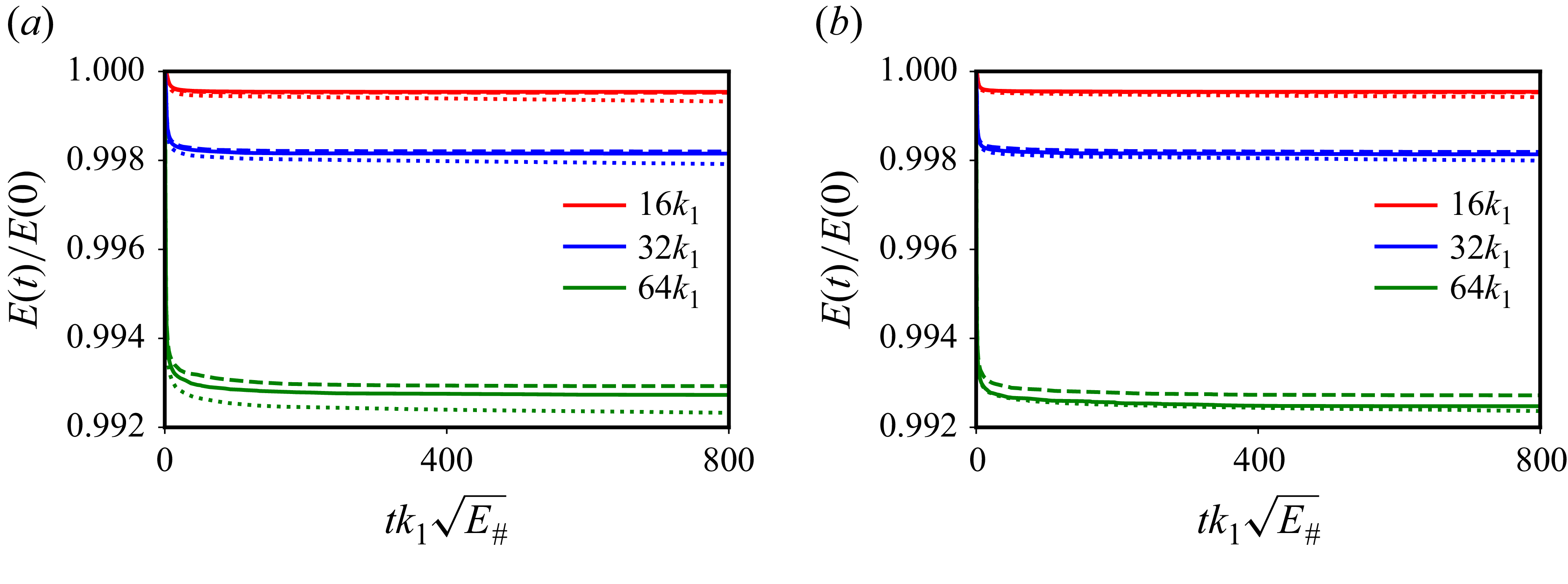
The time evolution of energy for various values of
 $\beta _s$
and
 $k_{\textit{ini}}$
for two initial energies,
 $0.25E_{\#}$
and
 $E_{\#}$
, are shown in figure 4. During the simulations,
 $0.8\,\%$
of the initial energy is lost for
 $k_{\textit{ini}}=64k_1$
and only
 $0.1\,\%$
for
 $k_{\textit{ini}} \leq 16k_1$
(see table 2 in Appendix B). Overall, energy is nearly conserved across all runs, which is essential for testing the minimum enstrophy hypothesis.
Time evolution of energy for
 $\beta _s=3.0$
(solid),
 $\beta _s=2.0$
(dashed) and
 $\beta _s=1.2$
(dotted) for (a)
 $E=0.25E_{\#}$
and (b)
 $E=E_{\#}$
runs with
 $k_{\textit{ini}}=16k_1, 32k_1$
and
 $64k_1$
.

Figure 5 illustrates the time evolution of enstrophy (
 $Q$
) for initial energy of
 $0.25 E_{\#}$
and
 $E_{\#}$
. In all cases, the enstrophy decreases significantly to a nearly constant, non-zero minimum value,
 $Q_f$
. Simulations with a large initial enstrophy (or high
 $k_{\textit{ini}}$
) lead to a correspondingly high final enstrophy value. However, enstrophy shows faster decay with a decrease in
 $\beta _s$
, irrespective of
 $k_{\textit{ini}}$
. Additionally, abrupt jumps in
 $Q$
appear in some simulations with initial energy
 $E\geq E_{\#}$
(see figure 5
b) due to the expulsion of filaments and subsequent decreases in enstrophy during vortex mergers. To quantitatively compare the deviation of the final enstrophy from the minimum enstrophy (
 $Q_*$
) predicted by variational principles, we plot
 $(Q_f-Q_*)/Q_{\eta }$
as a function of
 $\beta _s$
. This value tends to zero as
 $Q_f$
approaches
 $Q_*$
, indicating that the numerical solution approaches the MES. The inset of figure 5 shows that
 $(Q_f-Q_*)$
decreases with decrease in
 $\beta _s$
. Thus, the final enstrophy close to the theoretical enstrophy is obtained over a highly rough topography, irrespective of initial energy and length scale, thus underlining the importance of
 $\beta _s$
in the evolution of topographic turbulence.
Time evolution of enstrophy (
 $Q$
) for topographies with
 $\beta _s=3.0$
(solid),
 $2.0$
(dashed) and
 $1.2$
(dotted) for (a)
 $E=0.25E_{\#}$
runs and (b)
 $E=E_{\#}$
runs with
 $k_{\textit{ini}}=16k_1$
(red) and
 $k_{\textit{ini}}=64k_1$
(green). All vertical axes are in a symmetric log scale (linear within
 $[0,1]$
and logarithmic beyond it). Corresponding insets show
 $(Q_{f}-Q_*)/Q_{\eta }$
as a function of
 $\beta _s$
for
 $k_{\textit{ini}}=8k_1$
(yellow
 $\bullet$
),
 $16k_1$
(red
 $\bigstar$
),
 $32k_1$
(blue
 $\blacktriangledown$
) and
 $64k_1$
(green
 $\blacktriangle$
). The theoretical minimum enstrophy
 $Q_*$
obtained from (2.6).

3.2. Emergent structures and comparison with MES
The flow evolves from a random monoscale field, forming larger vortices via inverse cascade. Over time, the influence of topography becomes evident and the vorticity field adopts the shape of the topography. According to variational principles, a state of minimum enstrophy is characterised by a linear relationship between vorticity (
 $q_*$
) and the stream function (
 $\psi _*$
), expressed as
 $q_* = \mu \psi _*$
. In this section, we analyse the long-term snapshots of flow fields and verify to what extent they align with the linear relationship in three scenarios: first for the case of
 $E \ll E_{\#}$
, next for
 $E=E_{\#}$
and, finally, when
 $E \gg E_{\#}$
. The movies showing the time evolution of the flow field to long-term states are provided as supplementary movies available at https://doi.org/10.1017/jfm.2026.11455.
Figure 6 compares the snapshots for initial energy
 $0.25E_{\#}$
with the MES state for different values of
 $k_{\textit{ini}}$
and
 $\beta _s$
. For
 $\beta _s=3.0$
, strong vortices develop, where cyclones (anticyclones) are locked onto topographic elevations (depressions) with a non-uniform background PV (see figure 6
b and Movie S1). With increasing
 $k_{\textit{ini}}$
, more vortices form that exhibit higher mobility, resulting in a slightly homogenised background PV, similar to the findings of SY23 and HW24 (see figure 6
d and Movie S2). The presence of these long-lived vortices is the reason why the numerical solution deviates from the MES. However, with a decrease in
 $\beta _s$
, the size and intensity of these vortices decrease (see figures 6
f and 6
h and Movies S3, S4). Consequently, the flow evolves to a long-term state that closely resembles the MES for low
 $\beta _s$
.
Long-term snapshots (at
 $tk_1\sqrt {E_{\#}}=900$
) of
 $q$
field normalised with
 $\eta _{\textit{rms}}$
for simulations with initial energy
 $0.25E_{\#}$
, and
 $k_{\textit{ini}}=8k_1, 16k_1$
and
 $32k_1$
(second–fourth columns, respectively) compared with minimum enstrophy state (
 $q_*=\boldsymbol{\nabla} ^2\psi _* +\eta$
) (first column). Streamlines of
 $\psi _{*}$
are superimposed on all the plots. Top panels for
 $\beta _s=3.0$
and bottom panels for
 $\beta _s=1.2$
.

To quantify deviations from MES, we first construct scatter plots using the local values of
 $q/(k_1\sqrt {E_{\#}})$
and
 $k_1\psi /\sqrt {E_{\#}}$
obtained from numerical simulations. We then calculate the root mean square deviation defined as
 \begin{align} \varDelta = \sqrt { \langle |q-\mu \psi _*|^2 \rangle } \Big/ \big (k_1\sqrt {E_{\#}}\big ) \!. \end{align}
Figure 7 shows the comparison between MES and long-term flow fields for runs with initial energy
 $E=0.25E_{\#}$
. MES shows a linear relationship with a positive slope of
 $\mu /k_1^2=1.33$
for
 $\beta _s=3.0$
and
 $\mu /k_1^2=2.18$
for
 $\beta _s=1.2$
. Scatter plots of the long-term flow field for
 $\beta _s=3.0$
show branches, which are deviations from the straight line (see figure 7
b–d). These branches correspond to regions of intense cyclonic (
 $q\gt 0$
) and anticyclonic (
 $q\lt 0$
) vortices. The number and intensity of these branches increase with an increase in
 $k_{\textit{ini}}$
as more vortices are formed for large initial enstrophy. With a decrease in
 $\beta _s$
(see figure 7
f–h), the number and height of these branches predominantly decrease, indicating a reduction in the number and intensity of vortices. As a result, the deviation,
 $\varDelta$
, decreases with increasing roughness (small
 $\beta _s$
). This quantitatively confirms our observation that the long-term states closely resemble the MES for low
 $\beta _s$
.
Scatter plot at
 $tk_1\sqrt {E_{\#}}=900$
between
 $q/(k_1\sqrt {E_{\#}})$
and
 $k_1\psi /\sqrt {E_{\#}}$
for simulations with initial energy
 $0.25E_{\#}$
, and
 $k_{\textit{ini}}=8k_1, 16k_1$
and
 $32k_1$
(second–fourth columns, respectively) compared with MES (first column). MES solutions are shown in black as a straight line
 $q_*=\mu \psi _*$
, where
 $\mu$
is determined by energy
 $E=0.25E_{\#}$
and
 $\beta _s$
. Top panels for
 $\beta _s=3.0$
and bottom panels for
 $\beta _s=1.2$
.

Next, we examine the long-term flow fields with initial energy
 $E_{\#}$
, as shown in figure 8. For
 $\beta _s=3.0$
, vortices develop via inverse cascade and roam around the domain, leading to a homogenised background PV field (see figure 8
b and Movie S5). With the increase in
 $k_{\textit{ini}}$
, we observe the formation of numerous large intense vortices that move throughout the domain, often following the contours of
 $ \psi _{\#}$
(see figures 8
c and 8
d). As
 $\beta _s$
decreases, the intensity, size and mobility of vortices decrease, and for
 $\beta _s=1.2$
, we observe a slightly non-uniform background PV field for
 $k_{\textit{ini}}=8k_1$
due to the absence of vortices (see figure 8
f and Movie S6). As
 $k_{\textit{ini}}$
increases (to
 $32k_1$
), we observe tiny roaming vortices that lead to a homogenised background PV field (see figure 8
h and Movie S7). Figure 9 shows the comparison between scatter plots of MES and long-term flow fields for runs with initial energy
 $E=E_{\#}$
. At critical energy (
 $E=E_{\#}$
),
 $\mu =0$
and
 $q_*=0$
for all topographies. The long-term fields still show branches that reduce significantly at smaller
 $\beta _s=1.2$
, with the deviation (
 $\varDelta$
) reducing to half with increasing roughness.
Long-term snapshots (at
 $tk_1\sqrt {E_{\#}}=900$
) of
 $q$
field normalised with
 $\eta _{\textit{rms}}$
for simulations with initial energy
 $E_{\#}$
, and
 $k_{\textit{ini}}=8k_1, 16k_1$
and
 $32k_1$
(second–fourth columns, respectively) compared with minimum enstrophy state (
 $q_*=\boldsymbol{\nabla} ^2\psi _* +\eta$
) (first column). Streamlines of
 $\psi _{\#}$
are superimposed on all the plots. Top panels for
 $\beta _s=3.0$
and bottom panels for
 $\beta _s=1.2$
.

Scatter plot at
 $tk_1\sqrt {E_{\#}}=900$
between
 $q/(k_1\sqrt {E_{\#}})$
and
 $k_1\psi /\sqrt {E_{\#}}$
for simulations with initial energy
 $E_{\#}$
, and
 $k_{\textit{ini}}=8k_1, 16k_1$
and
 $32k_1$
(second–fourth columns, respectively) compared with MES (first column). MES solutions are shown in black as a straight line
 $q_*=\mu \psi _*$
, where
 $\mu$
is determined by energy
 $E=E_{\#}$
and
 $\beta _s$
. Top panels for
 $\beta _s=3.0$
and bottom panels for
 $\beta _s=1.2$
.

Finally, figure 10 presents long-term snapshots with initial energy
 $2E_{\#}$
. When
 $\beta _s=3.0$
, the vortices generated move freely across the domain, resulting in a homogeneous background PV for all values of
 $k_{\textit{ini}}$
(see figure 10
b–d and Movie S8). In contrast, for a
 $\beta _s=1.2$
, even though we observe a nearly homogenised background PV, the mobility of the vortices decreases significantly, resulting in cyclones rotating over topographic depressions and anticyclones over elevations for
 $k_{\textit{ini}} \leq 16k_1$
(see figures 10
f and 10
g and Movies S9, S10). For
 $k_{\textit{ini}} \geq 32k_1$
, the vortices detach from the topographic extremes and traverse the domain (see figure 10
h and Movie S11). Thus, locked vortices are still observed for rough topographies with flow initialised at length scales much smaller than the domain size and initial energy
 $E\gg E_{\#}$
. Figure 11 shows the comparison between MES and long-term flow fields for runs with initial energy
 $E=2E_{\#}$
. For
 $E\gg E_{\#}$
, MES shows a linear relationship between
 $q_*$
and
 $\psi _*$
with a negative slope (
 $\mu \lt 0$
). Similar to figures 7 and 9, long-term fields still show branches which reduce significantly at smaller
 $\beta _s=1.2$
.
Long-term snapshots (at
 $tk_1\sqrt {E_{\#}}=900$
) of
 $q$
field normalised with
 $\eta _{\textit{rms}}$
for simulations with initial energy
 $2E_{\#}$
, and
 $k_{\textit{ini}}=8k_1, 16k_1$
and
 $32k_1$
(second–fourth columns, respectively) compared with minimum enstrophy state (
 $q_*=\boldsymbol{\nabla} ^2\psi _* +\eta$
) (first column). Streamlines of
 $\psi _{*}$
are superimposed on all the plots. Top panels for
 $\beta _s=3.0$
and bottom panels for
 $\beta _s=1.2$
.

Scatter plot at
 $tk_1\sqrt {E_{\#}}=900$
between
 $q/(k_1\sqrt {E_{\#}})$
and
 $k_1\psi /\sqrt {E_{\#}}$
for simulations with initial energy
 $2E_{\#}$
, and
 $k_{\textit{ini}}=8k_1, 16k_1$
and
 $32k_1$
(second–fourth columns, respectively) compared with MES (first column). MES solutions are shown in black as a straight line
 $q_*=\mu \psi _*$
, where
 $\mu$
is determined by energy
 $E=2E_{\#}$
and
 $\beta _s$
. Top panels for
 $\beta _s=3.0$
and bottom panels for
 $\beta _s=1.2$
.

The relative vorticity field corresponding to figures 6, 8 and 10 is given in Appendix C. Thus, in a nutshell, we observe that the number, size and mobility of the vortices decrease with a decrease in
 $\beta _s$
. Consequently, at small
 $\beta _s$
, the long-term state resembles the MES for
 $E \ll E_{\#}$
and vortices are locked onto the topographic extrema for
 $E \gg E_{\#}$
.
3.3. Spectral properties of flow field
In the absence of external forcing, 2-D turbulence over topography is characterised by a self-organising process in which energy cascades from small to larger scales (an inverse energy cascade), eventually halting as the flow tends towards a steady state aligned with the topographic contours.
The long-term energy spectra for different values of
 $k_{\textit{ini}}$
for
 $E=0.25E_{\#}$
along with the energy spectra of MES over two topographies, are shown in figure 12. For
 $\beta _s=3.0$
, as shown in figure 12(a), the MES spectra scales as
 $k^{-5}$
. However, the long-term energy spectra do not collapse onto the MES prediction and show a substantial offset from MES. This offset increases with an increase in
 $k_{\textit{ini}}$
. For
 $\beta _s=3.0$
, the observed scaling in the long-term spectra for all the
 $k_{\textit{ini}}$
values is slightly shallower than the MES slope. However, for
 $\beta _s=1.2$
, as shown in figure 12(b), the long-term energy spectra agree more closely with the MES spectra, particularly at small scales. It is interesting to note that, irrespective of
 $k_{\textit{ini}}$
, deviations from MES are uniform across all scales for
 $\beta _s=3.0$
, while a selective deviation at large scales is observed for
 $\beta _s=1.2$
. These selective deviations are due to the presence of vortices for high
 $k_{\textit{ini}}$
.
Long-term energy spectra for runs with initial energy,
 $E=0.25E_{\#}$
, and
 $k_{\textit{ini}}=8k_1$
(yellow),
 $16k_1$
(red),
 $32k_1$
(blue) and
 $64k_1$
(green) over topography with (a)
 $\beta _s=3.0$
and (b)
 $\beta _s=1.2$
. The black line is the MES spectra obtained from variational principles, with slope
 $k^{-(\beta _s+2)}$
(dashed line). Insets show the time evolution of normalised characteristic wavenumber,
 $k_c/k_{\textit{ini}}$
(dotted lines), for runs with different values of
 $k_{\textit{ini}}$
.

The insets of figure 12 show the time evolution of a characteristic wavenumber,
 $k_c=\int k\mathcal{E}(k)\,\text{d}k/E$
. The decrease in
 $k_c$
from
 $k_{\textit{ini}}$
can be attributed to the inverse cascade of energy from small scales to large scales. Note that
 $k_c$
decreases to a constant value over time, indicating an arrest in the inverse cascade as the flow matches the topography.
The analogy between topographic turbulence and
 $\beta$
-plane turbulence has been of interest for decades (Vallis & Maltrud Reference Vallis and Maltrud1993; Constantinou & Young Reference Constantinou and Young2017). An arrest of inverse cascade also occurs in
 $\beta$
-plane turbulence when the characteristic wavenumber approaches the Rhines wavenumber. It has been observed that the time taken for
 $k_c$
to reach the Rhines wavenumber is independent of
 $k_{\textit{ini}}$
when
 $k_{\textit{ini}}$
is much larger than the Rhines wavenumber (Rhines Reference Rhines1975). If
 $k_{\textit{ini}}$
is much less than the Rhines wavenumber, the flow is aware of the
 $\beta$
effect from the start and the flow evolution is sensitive to initial conditions (see supplementary material for details). In topographic turbulence, we observe that the final flow fields and their spectral properties are dependent on
 $k_{\textit{ini}}$
irrespective of the roughness of the topography. This could point to certain similarities between the two systems.
3.4. Correlations
Following SY23, we systematically calculate two correlation measures to analyse the presence of locked and roaming vortices. The first correlation,
 $C_{\zeta \eta } = \langle \zeta \eta \rangle / \sqrt {\langle \zeta ^2 \rangle \langle \eta ^2 \rangle }$
, measures how closely relative vorticity (
 $\zeta$
) aligns with
 $\eta$
, where
 $ C_{\zeta \eta }$
can reach as low as
 $ -1$
. The second correlation,
 $C_{q\psi _\#} = \langle q \psi _\# \rangle / \sqrt {\langle q^2 \rangle \langle \psi _{\#}^2 \rangle }$
, is between MES solution
 $\psi _{\#}$
and
 $q$
. In the vicinity of
 $E_{\#}$
, the variational principle yields
 $q\approx \mu \psi _\#$
implying
 $C_{q\psi _\#}=\mu /|\mu |$
. As
 $\mu \gt 0$
for
 $E/E_{\#}\lt 1$
and
 $\mu \lt 0$
for
 $E/E_{\#}\gt 1$
, the sign of
 $ C_{q\psi _\#}$
is sensitive to the energy level, transitioning from +1 to −1 at
 $ E_{\#}$
.
Figure 13 illustrates the time evolution of
 $C_{\zeta \eta }$
and
 $C_{q\psi _\#}$
for different values of
 $\beta _s$
and
 $k_{\textit{ini}}$
. Initially (at
 $t=0$
), the fields are uncorrelated. As the flow progresses,
 $C_{\zeta \eta }$
(see
 $\bullet$
points in figures 13
a and 13
b) decreases as the relative vorticity fields adapt to the shape of the topography. However, numerical results show the presence of vortices in the flow field, due to which
 $C_{\zeta \eta }$
is larger than
 $-1$
. However, regardless of the initial energy and
 $k_{\textit{ini}}$
, the correlation decreases with a decrease in
 $\beta _s$
. This variation is attributed to the decrease in vortex size and intensity with increasing topographic roughness.
Time evolution of correlation coefficients
 $C_{\zeta \eta }$
(
 ${\bullet}$
) and
 $C_{q \psi _{\#}}$
(
 $\blacksquare$
) with initial energies (a)
 $0.25E_{\#}$
, (b)
 $E_{\#}$
. Solid lines for
 $\beta _s=3.0$
and dotted for
 $\beta _s=1.2$
. Colours for
 $8k_1$
(magenta) and
 $32k_1$
(blue).

The second correlation,
 $C_{q\psi _\#}$
(see
 $\blacksquare$
points in figure 13
a), increases to a positive value with time for
 $E\ll E_{\#}$
, indicating a non-uniform background PV due to the presence of locked vortices. As
 $k_{\textit{ini}}$
increases, the long-term correlation decreases because the vortices, though locked, become more mobile, resulting in a slightly homogenised background PV.
For
 $E=E_{\#}$
,
 $C_{q\psi _\#}$
is close to zero, indicating homogenised background PV due to roaming vortices (see
 $\blacksquare$
points in figure 13
b). Interestingly, for lower
 $\beta _s$
and intermediate
 $k_{\textit{ini}}$
(
 $=8k_1$
),
 $C_{q\psi _\#}$
is greater than zero, suggesting less mobile vortices and a slightly non-uniform background PV, which is also supported by the snapshot in figure 8(f). Similar behaviour is observed for
 $E\gt E_{\#}$
. Thus, the interplay between initially specified energy and topographic roughness strongly governs whether turbulent flows organise into locked vortices with a non-uniform background PV field or evolve into roaming vortices with an homogenised background PV field.
4. Conclusion and discussion
We show that long-term flow states of weakly decaying quasi-geostrophic two-dimensional turbulence over topography, initiated by monoscale fields of different length scales and energy, depend strongly on the roughness (
 $\beta _s$
) of the topography. As
 $\beta _s$
decreases, the number, mobility and intensity of vortices in the flow field decrease. The long-term flow field on topography with high roughness (low
 $\beta _s$
) better matches with MES when
 $E \ll E_{\#}$
. For
 $E \gg E_{\#}$
, we observe vortices roaming around the domain when topography has smoother structures (high
 $\beta _s$
). Interestingly, decreasing
 $\beta _s$
restricts the vortex mobility, thereby restricting it to the topographic extrema. Our findings highlight the sensitivity of topographic turbulence to the spectral nature of topography and underscore the need for a more thorough integration of realistic oceanic topographies, particularly those exhibiting varying spectral slope characteristics, into numerical and analytical models of geophysical turbulence.
We conclude by drawing an analogy between
 $\beta$
-plane turbulence and topographic turbulence, which stems from the fact that both differential rotation and topography imply a gradient of PV. While the planetary PV gradient (
 $\beta$
) is responsible for the formation of zonal jets (Rhines Reference Rhines1975), the gradient of topographic PV can cause the mean flow oriented parallel to the topographic contours to become organised into jets (Vallis & Maltrud Reference Vallis and Maltrud1993). Unlike the constant planetary PV gradient used in
 $\beta$
-plane turbulence, the topographic PV gradient here is complex and spatially varying. Thus, understanding the similarities and differences between topographic turbulence and
 $\beta$
-plane turbulence is of considerable interest. Consequently, a systematic study of
 $\beta$
-plane turbulence over rough topography is a promising direction for future work.
Supplementary material and movies
Movies for the chosen parameters and an analogy with
 $\beta$
-plane turbulence. Supplementary material and movies are available at https://doi.org/10.1017/jfm.2026.11455.
Acknowledgements
We gratefully acknowledge Professor W. R. Young (Scripps Institution of Oceanography), Professor J. C. McWilliams (University of California, Los Angeles) and Professor P. L. Read (University of Oxford) for their pioneering contributions to planetary and geophysical fluid dynamics, which have been a constant source of inspiration for the present work. We also thank Professor E. Guazzelli (CNRS, France) for insightful discussions and valuable suggestions that have enriched this study and our broader perspective on fluid mechanics. We are especially indebted to the three anonymous referees for their careful reading of the manuscript and for their constructive and insightful comments, which have substantially improved the clarity, rigour and overall presentation of this work. We sincerely thank P. Shakti for the computing resources developed under the National Supercomputing Mission, India.
Funding
V.R.K.P. gratefully acknowledges the research support from the Prime Minister’s Research Fellows Scheme, Government of India.
Declaration of interests
The authors report no conflict of interest.
Appendix A. Grid independence
The largest wavenumber resolved by our pseudospectral simulation with a
 $N\times N$
grid is given by
 $(N/2)k_1$
. The dissipation term used is a high-wavenumber filter with
 $k_{\textit{cutoff}}=(N/3)k_1$
(see (2.9) in the manuscript). Note that the topographic spectrum is tapered to zero at the
 $k_{\textit{cutoff}}-150k_1$
, ensuring that dissipation removes only flow features at scales smaller than the topographic scales. In this way, the topography does not excite energy at scales smaller than the dissipation scales. We simulated certain parameter cases with a grid resolution of
 $4096 \times 4096$
and compared with
 $2048\times 2048$
to understand the influence of a wider topographic spectrum. Figure 14(a) shows the time evolution of enstrophy on two grids for simulations on topography with
 $\beta _s=3.0$
and
 $\beta _s=1.2$
. Apart from the slight differences that arise from the difference in randomness of the initial vorticity field, which influences the vortex-merging process, the enstrophy decay matches to a good extent. Note that the long-term energy spectra (
 $tk_1\sqrt {E_{\#}}=900$
) are almost identical in both grids, as shown in the inset of figure 14(a). Since doubling the resolution does not change our conclusions and the relative effect of topography is nevertheless captured, we use
 $2048 \times 2048$
for our study.
(a) Evolution of normalised enstrophy of run with initial wavenumber,
 $k_{\textit{ini}}=16k_1$
, initial energy,
 $E=0.25E_{\#}$
, using two different grids,
 $2048 \times 2048$
(solid line) and
 $4096 \times 4096$
(
 $\unicode{x2B24}$
) on topography with
 $\beta _s=3.0$
(blue) and
 $\beta _s=1.2$
(red). The inset shows the energy spectra at the final time (
 $tk_1\sqrt {E_{\#}}=900$
) for two grid resolutions for
 $\beta _s=3.0$
. (b) Normalised initial enstrophy
 $Q(0)$
versus
 $k_{\textit{ini}}$
for different values of topographic roughness,
 $\beta _s$
. Circles for
 $E=0.25E_{\#}$
and squares for
 $E=E_{\#}$
.

Appendix B. Initial conditions and energy conservation
The computations are initialised with a random monoscale relative vorticity field,
 $\zeta (x,y)$
, characterised by a single well-defined length scale,
 $2\pi /k_{\textit{ini}}$
, as shown in figure 15. The larger the
 $k_{\textit{ini}}$
, the smaller the length scale associated with the initial field. In non-dimensional variables, the initial enstrophy,
 $Q(0)$
estimated by SY23, is
 \begin{align} \frac {Q(0)}{Q_{\eta }}= \underbrace {\left ( \frac {k_{\textit{ini}}}{k_1} \right )^2}_{\text{I}} \underbrace {\frac {k_1^2 E_{\#}}{Q_\eta }}_{\text{II}} \underbrace {\frac {E}{E_{\#}}}_{\text{III}} +1, \end{align}
where the term
 $\text{I}$
shows the dependence of
 $Q(0)$
on
 $k_{\textit{ini}}$
, term
 $\text{II}$
shows the dependence on topography indirectly via
 $E_{\#}$
and term
 $\text{III}$
on non-dimensional energy
 $E/E_{\#}$
. The initial enstrophy for different combinations of
 $\beta _s$
,
 $k_{\textit{ini}}$
and
 $E/E_{\#}$
is shown in figure 14(b). For a given normalised energy
 $E/E_{\#}$
and
 $\beta _s$
,
 $Q(0)$
increases at a rate of approximately
 $k_{\textit{ini}}^2$
(He & Wang Reference He and Wang2024). The larger the
 $k_{\textit{ini}}$
, the larger the initial enstrophy.
Normalised initial relative vorticity field (
 $\zeta /\eta _{\textit{rms}}$
): (a)
 $k_{\textit{ini}}=8k_1$
; (b)
 $k_{\textit{ini}}=16k_1$
; (c)
 $k_{\textit{ini}}=32k_1$
and (d)
 $k_{\textit{ini}}=64k_1$
.

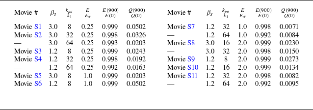
Kinetic energy is almost conserved throughout the evolution of the
 $150$
simulations carried out for this study. The normalised energy and enstrophy at end of simulation (
 $tk_1\sqrt {E_\#} = 900$
) are shown in table 2.
Movie numbers (column 1) corresponding to the runs with different values of
 $\beta _s$
(column 2),
 $k_{\textit{ini}}/k_1$
(column 3) and
 $E/E_{\#}$
(column 4), normalised kinetic energy
 $E/E(0)$
(column 5) and normalised potential enstrophy
 $Q/Q(0)$
(column 6) at time
 $tk_1\sqrt {E_\#} = 900$
. The movies are uploaded as ‘Movie
 $\#$
_beta_xx_k_xx_En_xx’, where beta is for
 $\beta _s$
value, k for
 $k_{\textit{ini}}$
and En for
 $E/E_{\#}$
.

Appendix C. Relative vorticity fields
The long-term relative vorticity fields for different values of
 $\beta _s$
,
 $k_{\textit{ini}}$
and
 $E$
are shown in figure 16 (for
 $E \ll E_{\#}$
), figure 17 (for
 $E=E_{\#}$
) and figure 18 (for
 $E \gg E_{\#}$
), respectively. For
 $E \ll E_{\#}$
, the long-term fields show large topographically locked vortices for
 $\beta _s=3.0$
, which nucleate to create more vortices with an increase in
 $k_{\textit{ini}}$
(see figures 16
c and 16
g). In the case of
 $\beta _s=1.2$
, the long-term fields resemble the minimum enstrophy solution (MES) for
 $k_{\textit{ini}} \lt 16k_1$
, while small topographically locked vortices are observed when
 $k_{\textit{ini}} \geq 16k_1$
(see figures 16
dand 16
h).
Long term snapshots of relative vorticity field of
 $E=0.25E_{\#}$
for
 $k_{\textit{ini}}=8k_1, 16k_1$
and
 $32k_1$
(second–fourth columns, respectively) compared with MES (first column) for
 $\beta _s=3.0$
(a,c,e,g) and
 $\beta _s=1.2$
(b,d,f,h).

Long-term snapshots of relative vorticity field of
 $E=E_{\#}$
for
 $k_{\textit{ini}}=8k_1, 16k_1$
and
 $32k_1$
(second–fourth columns, respectively) compared with MES (first column) for
 $\beta _s=3.0$
(a,c,e,g) and
 $\beta _s=1.2$
(b,d,f,h).

Long-term snapshots of relative vorticity field of
 $E=2E_{\#}$
for
 $k_{\textit{ini}}=8k_1, 16k_1$
and
 $32k_1$
(second–fourth columns, respectively) compared with MES (first column) for
 $\beta _s=3.0$
(a,c,e,g) and
 $\beta _s=1.2$
(b,d,f,h).

For
 $E=E_{\#}$
, we observe long-term states showing large vortices roaming around the domain for
 $\beta _s=3.0$
, whereas for
 $\beta _s=1.2$
, in addition to the background field resembling MES, we observe tiny blobs of vortices roaming the domain for
 $k_{\textit{ini}} \gt 16k_1$
(see figure 17 and the corresponding supplementary movies).
For
 $E \gg E_{\#}$
, we observe large vortices roaming around the domain for
 $\beta _s=3.0$
irrespective of the initial wavenumber, while they are topographically locked for
 $\beta _s=1.2$
when
 $k_{\textit{ini}}\leq 16k_1$
(see figures 18
e and 18
f). When
 $k_{\textit{ini}} \gt 16k_1$
, these vortices nucleate and roam around the domain for
 $\beta _s=1.2$
(see the corresponding supplementary movies).