



1 Introduction
Stability and sensitivity analysis of a flow configuration (base flow) is important both for investigating the path followed by the flow to depart from the selected configuration when this is unstable and for the identification of possible controls of an identified instability. Passive controls generally lead to ad hoc modifications of the base flow which change its stability properties in a desired way. In particular, the dynamics of small disturbances superimposed onto the reference state is modified by passive control in two ways: (i) by a modification of the base flow, and (ii) by a direct action of the control on the dynamics itself. This aspect is well illustrated for instance in Marquet, Sipp & Jacquin (Reference Marquet, Sipp and Jacquin2008) and Luchini, Giannetti & Pralits (Reference Luchini, Giannetti and Pralits2009), where stability and sensitivity analysis is applied to investigate the passive control of the vortex shedding instability in the wake past a circular cylinder exerted by using a small control rod positioned in the wake. In Marquet et al. (Reference Marquet, Sipp and Jacquin2008) it is shown that the two contributions of the control, i.e. the modification of the base flow and its direct action on the disturbance dynamics, both play an important role in the modification of the instability. Moreover, a strategy is proposed so as to derive control maps predicting the effect of the control rod for a generic position of its centre using adjoint methods. The same idea and methods have been successively applied in the literature to a wide variety of flow instabilities (see, for instance, the review in Camarri (Reference Camarri2015)).
A key ingredient in the method proposed in Marquet et al. (Reference Marquet, Sipp and Jacquin2008) is the sensitivity analysis of a selected global instability to a variation of the base flow which can be induced by a generic forcing of the momentum equations. This aspect alone, even without the implications it may have for control purposes, plays a significant role in the characterisation of the instability, as also underlined in Sipp et al. (Reference Sipp, Marquet, Meliga and Barbagallo2010), Luchini & Bottaro (Reference Luchini and Bottaro2014) and Camarri (Reference Camarri2015).
The first sensitivity analysis to a base-flow modification is documented in Bottaro, Corbett & Luchini (Reference Bottaro, Corbett and Luchini2003), where the authors assessed the sensitivity of the Orr–Sommerfeld spectrum to a generic modification of the base flow for plane Couette flow. They used variational techniques to determine the mean-flow modification of prescribed magnitude having the largest effect on a selected eigenmode. Small base-flow variations were found to be sufficient to destabilise the flow that is otherwise unconditionally stable according to linear stability analysis, this last aspect being in contrast to experimental evidence. Gavarini, Bottaro & Nieuwstadt (Reference Gavarini, Bottaro and Nieuwstadt2004) studied the effect of base-flow distortions in the transition process of cylindrical pipe flows. The sensitivity of the singular values of the resolvent operator of the linearised flow dynamics with respect to base-flow modifications was studied by Brandt et al. (Reference Brandt, Sipp, Pralits and Marquet2011), who derived the analytical expression for the gradient of the resolvent norm of the system with respect to the base-flow modifications. However, sensitivity analysis to base-flow modifications is also relevant for configurations in which the base flow is periodic in time. Almost all the studies documented in the literature on sensitivity analysis to base-flow perturbations, and in particular all the references cited above, consider steady base flows. There are, however, a few examples of sensitivity-based controls for time-periodic base flows. For instance, in Meliga et al. (Reference Meliga, Boujo, Pujals and Gallaire2014) a sensitivity analysis of the time-averaged drag coefficient for the periodic flow past a square cylinder at Reynolds number
 $Re=100$
is carried out by integrating backwards in time an adjoint problem depending on the time history of the flow. The resulting theoretical framework allows one to predict the effect on the mean drag of a small control wire generically positioned in the flow. A less CPU-demanding approach for the same control maps is proposed in Meliga, Boujo & Gallaire (Reference Meliga, Boujo and Gallaire2016) and analysed in detail in Meliga (Reference Meliga2017). This last method consists of an adjoint-based analysis of the self-consistent model for vortex shedding proposed in Mantič-Lugo, Arratia & Gallaire (Reference Mantič-Lugo, Arratia and Gallaire2014), which results in solving a steady nonlinear adjoint problem. The results provided are shown to be accurate and less CPU-demanding than the time-stepping analysis proposed in Meliga et al. (Reference Meliga, Boujo, Pujals and Gallaire2014).
Besides sensitivity-based controls of the limit cycle in a time-periodic base flow, it is also interesting to consider controls of the instabilities that can arise in such a base flow. Indeed, several important flow instabilities can arise in this case, as for instance the secondary instability occurring in plane wakes past bluff bodies leading the flow from a two- (2D) to a three-dimensional (3D) state. A partial result in this respect is documented in Giannetti, Camarri & Luchini (Reference Giannetti, Camarri and Luchini2010), where the sensitivity of the 3D secondary instability of the wake of a circular cylinder to a structural perturbation of the linearised Navier–Stokes equations is investigated by adjoint methods. To this purpose, the work in Giannetti et al. (Reference Giannetti, Camarri and Luchini2010) generalises the approach originally proposed by Giannetti & Luchini (Reference Giannetti and Luchini2007) to investigate the first instability of the cylinder wake so as to include the case of time-periodic base flows. In particular, the authors identify a localised region of maximum coupling among the velocity components by using the direct and adjoint Floquet mode associated with the selected 3D instability. The resulting sensitivity field takes into account the feedback which is at the origin of the self-excited oscillation and is therefore useful to locate the region where the instability mechanism acts. However, the theoretical approach proposed in Giannetti et al. (Reference Giannetti, Camarri and Luchini2010) investigates only one of the two ways in which the dynamics of small perturbations on a time-periodic base flow can be affected by a passive control, i.e. by a direct action of a control on the disturbance dynamics. The second way in which the control can interfere with the instability is by a modification of the base flow, and this aspect, which is the main objective of the present work, has not been investigated in the literature before. In this respect the work in Giannetti et al. (Reference Giannetti, Camarri and Luchini2010) and the theory which is proposed here are complementary and both necessary to estimate the effect of a passive control of an instability developing on a time-periodic base flow. Since we work here in a linearised framework, the results provided by the theory in Giannetti et al. (Reference Giannetti, Camarri and Luchini2010) can be summed directly to the ones provided by the theory proposed here, so as to overlap the two effects of a flow control just mentioned in order to derive control maps for an identified instability. As a result the framework proposed here provides a tool to design passive controls for instabilities developing on a time-periodic base flow.
As an example of application of the proposed theory, we consider the well-known 3D instability of the wake past a circular cylinder, which is an important paradigmatic instability and, for this reason, is widely investigated in the literature. Concisely, Noack, König & Eckelmann (Reference Noack, König and Eckelmann1993) and Noak & Eckelmann (Reference Noak and Eckelmann1994) found that the flow past a circular cylinder is unstable to 3D perturbations when the flow Reynolds number exceeds a given threshold. Successively, accurate numerical simulations carried out by Barkley & Henderson (Reference Barkley and Henderson1996) confirmed the existence of two separate bands of synchronous unstable modes: mode A (
 $Re_{cr}^{A}=189$
), which is characterised by a spanwise wavelength of approximately four cylinder diameters, and mode B (
 $Re_{cr}^{B}=259$
), which has a spanwise wavelength of approximately one diameter. Direct numerical simulations (DNS) and experimental investigations confirm the existence of these instabilities (Williamson Reference Williamson1988). In such a context, the sensitivity analysis carried out here, besides being an example of application of the proposed theory, also provides new and important information pertaining to the nature and the control of the secondary instability in the wake past a circular cylinder. Moreover, control maps are derived and validated, and they are shown to be in excellent agreement with the experiments documented in Zhang, Fey & Noack (Reference Zhang, Fey and Noack1995).
Despite the particular application detailed here, the formulation proposed is general and can be used without any conceptual difficulty to analyse generic base flows that are periodic in time.
After having introduced the problem of the secondary instability in the wake past a circular cylinder and concisely recalled the Floquet stability analysis in § 2, we present the original method proposed here in § 3. In § 4 we merge the results obtained here with those in Giannetti et al. (Reference Giannetti, Camarri and Luchini2010) and, as a result, we provide the tools for estimating the effect of a local force–velocity feedback, which may mimic, for instance, the effect of a control wire as used in Zhang et al. (Reference Zhang, Fey and Noack1995), on the secondary instability. Using the numerical methods described in § 5, we show the original results obtained for the cylinder wake in § 6.
2 Flow configuration and Floquet analysis
In this section, after having introduced the considered flow configuration, we concisely describe the tools for investigating the stability analysis of a time-periodic base flow by a Floquet analysis.
2.1 Flow configuration
The incompressible flow around a nominally 2D circular cylinder is considered here and the theory is presented focusing on this specific case, as discussed in the introduction. The flow is described using a Cartesian coordinate system with the
 $z$
-axis coinciding with the cylinder axis and with the
 $x$
-axis aligned with the direction of the incoming uniform flow. The flow is governed by the unsteady incompressible Navier–Stokes equations, which are made dimensionless using the cylinder diameter
 $D^{\ast }$
as the characteristic length scale, the velocity of the incoming stream
 $U_{\infty }^{\ast }$
as the reference velocity, and the (constant) fluid density
 $\unicode[STIX]{x1D70C}^{\ast }$
:
 $$\begin{eqnarray}\displaystyle & \displaystyle {\displaystyle \frac{\unicode[STIX]{x2202}\boldsymbol{U}}{\unicode[STIX]{x2202}t}}+\boldsymbol{U}\boldsymbol{\cdot }\unicode[STIX]{x1D735}\boldsymbol{U}=-\unicode[STIX]{x1D735}P+{\displaystyle \frac{1}{Re}}\unicode[STIX]{x1D6AB}\boldsymbol{U}, & \displaystyle\end{eqnarray}$$
 $$\begin{eqnarray}\displaystyle & \displaystyle \unicode[STIX]{x1D735}\boldsymbol{\cdot }\boldsymbol{U}=0, & \displaystyle\end{eqnarray}$$
 $\boldsymbol{U}$
is the normalised velocity vector with components
 $\boldsymbol{U}=(U,V,W)$
,
 $P$
is the reduced pressure and
 $Re=U_{\infty }^{\ast }D^{\ast }/\unicode[STIX]{x1D708}^{\ast }$
is the Reynolds number (
 $\unicode[STIX]{x1D708}^{\ast }$
being the kinematic viscosity of the fluid). As for the boundary conditions of the continuous problem, no-slip and no-penetration conditions are applied on the cylinder surface
 $\unicode[STIX]{x1D6E4}_{c}$
and the flow is assumed to asymptotically approach the incoming uniform stream in the far field.
2.2 Floquet analysis
The considered flow becomes periodic in time when the Reynolds number exceeds a critical value
 $Re_{c1}\approx 47$
, as widely investigated in the literature. The 3D instability occurring in the resulting time-periodic wake can be investigated using Floquet theory (see e.g. Drazin Reference Drazin2002), which is now concisely described.
The Floquet analysis is carried out in order to investigate the stability properties of a time-periodic solution of (2.1),
 $\boldsymbol{Q}_{b}=(\boldsymbol{U}_{b},P_{b})$
of period
 $T$
. In the specific case of the considered wake,
 $\boldsymbol{Q}_{b}$
is also a planar 2D flow in the
 $x{-}y$
plane. Thus we have
 $\boldsymbol{Q}_{b}(x,y,t+T)=\boldsymbol{Q}_{b}(x,y,t)$
and
 $\boldsymbol{U}_{b}\boldsymbol{\cdot }\boldsymbol{e}_{z}=0$
,
 $\boldsymbol{e}_{z}$
begin the versor of the
 $z$
-direction. It is assumed that a generic unsteady and 3D perturbation is superimposed onto the base flow
 $\boldsymbol{Q}_{b}$
, thus leading to the total flow field
 $\boldsymbol{Q}=\{\boldsymbol{U},P\}$
:
 $$\begin{eqnarray}\displaystyle & \displaystyle \boldsymbol{U}(x,y,z,t)=\boldsymbol{U}_{b}(x,y,t)+\unicode[STIX]{x1D716}{\displaystyle \frac{1}{\sqrt{2\unicode[STIX]{x03C0}}}}\displaystyle \int _{-\infty }^{\infty }\boldsymbol{u}(x,y,k,t)\exp (\text{i}kz)\,\text{d}k, & \displaystyle\end{eqnarray}$$
 $$\begin{eqnarray}\displaystyle & \displaystyle P(x,y,z,t)=P_{b}(x,y,t)+\unicode[STIX]{x1D716}{\displaystyle \frac{1}{\sqrt{2\unicode[STIX]{x03C0}}}}\displaystyle \int _{-\infty }^{\infty }p(x,y,k,t)\exp (\text{i}kz)\,\text{d}k, & \displaystyle\end{eqnarray}$$
 $\unicode[STIX]{x1D716}$
is the disturbance amplitude and
 $\boldsymbol{u}$
and
 $p$
are the velocity and pressure disturbances Fourier-transformed in the spanwise direction (a homogeneous direction for the base flow). Introducing (2.2) in (2.1) and linearising in
 $\unicode[STIX]{x1D716}$
, we obtain two problems describing, respectively, the evolution of the 2D periodic base flow and the dynamics of the 3D perturbations. In particular, the base flow is governed by the 2D version of (2.1), while the perturbation field is described by the 3D unsteady linearised Navier–Stokes equations (LNSE). When the Fourier transform in the
 $z$
-direction is applied to the LNSE, for each wavenumber
 $k$
the following set of equations is obtained:
 $$\begin{eqnarray}\displaystyle & \displaystyle \frac{\unicode[STIX]{x2202}\boldsymbol{u}}{\unicode[STIX]{x2202}t}+\unicode[STIX]{x1D647}_{k}\{\boldsymbol{U}_{b},Re\}\boldsymbol{u}+\unicode[STIX]{x1D735}_{k}p=\mathbf{0}, & \displaystyle\end{eqnarray}$$
 $$\begin{eqnarray}\displaystyle & \displaystyle \unicode[STIX]{x1D735}_{k}\boldsymbol{\cdot }\boldsymbol{u}=0, & \displaystyle\end{eqnarray}$$
 $\unicode[STIX]{x1D735}_{k}\equiv (\unicode[STIX]{x2202}/\unicode[STIX]{x2202}x,\unicode[STIX]{x2202}/\unicode[STIX]{x2202}y,\text{i}k)$
is the Fourier-transformed gradient operator,
 $\unicode[STIX]{x1D647}_{k}$
stands for the Fourier-transformed linearised Navier–Stokes operator,
 $$\begin{eqnarray}\unicode[STIX]{x1D647}_{k}\{\boldsymbol{U}_{b},Re\}\boldsymbol{u}=\boldsymbol{U}_{b}\boldsymbol{\cdot }\unicode[STIX]{x1D735}_{k}\boldsymbol{u}+\boldsymbol{u}\boldsymbol{\cdot }\unicode[STIX]{x1D735}_{k}\boldsymbol{U}_{b}-{\displaystyle \frac{1}{Re}}\unicode[STIX]{x1D6AB}_{k}\boldsymbol{u},\end{eqnarray}$$
and
 $\unicode[STIX]{x1D6AB}_{k}\equiv \unicode[STIX]{x1D735}_{k}\boldsymbol{\cdot }\unicode[STIX]{x1D735}_{k}$
is the Fourier-transformed Laplacian operator. In the Floquet stability analysis, the linearised flow field
 $\boldsymbol{q}=\{\boldsymbol{u},p\}$
is further assumed to have the following modal form:
 $$\begin{eqnarray}\boldsymbol{q}(x,y,k,t)=\hat{\boldsymbol{q}}(x,y,k,t)\exp (\unicode[STIX]{x1D70E}t),\end{eqnarray}$$
where
 $\unicode[STIX]{x1D70E}$
is the Floquet exponent while
 $\hat{\boldsymbol{q}}=\{\hat{\boldsymbol{u}},\hat{p}\}$
is a non-trivial periodic field, with the same period
 $T$
as the base flow, i.e.
 $\hat{\boldsymbol{q}}(x,y,k,t+T)=\hat{\boldsymbol{q}}(x,y,k,t)$
.
Substituting the modal form of the disturbance, equation (2.5), in (2.3), it is found that
 $\hat{\boldsymbol{q}}$
satisfies the following set of equations:
 $$\begin{eqnarray}\displaystyle & \displaystyle {\displaystyle \frac{\unicode[STIX]{x2202}\hat{\boldsymbol{u}}}{\unicode[STIX]{x2202}t}}+\unicode[STIX]{x1D70E}\hat{\boldsymbol{u}}+\unicode[STIX]{x1D647}_{k}\{\boldsymbol{U}_{b},Re\}\hat{\boldsymbol{u}}+\unicode[STIX]{x1D735}_{k}\hat{p}=\mathbf{0}, & \displaystyle\end{eqnarray}$$
 $$\begin{eqnarray}\displaystyle & \displaystyle \unicode[STIX]{x1D735}_{k}\boldsymbol{\cdot }\hat{\boldsymbol{u}}=0, & \displaystyle\end{eqnarray}$$
 $$\begin{eqnarray}\hat{\boldsymbol{q}}=\{\hat{\boldsymbol{u}},\hat{p}\}\rightarrow \{\mathbf{0},0\}\quad \text{as}\;r\rightarrow \infty .\end{eqnarray}$$
The system of equations (2.6) along with the above boundary conditions and the periodicity requirement for the solution
 $\hat{\boldsymbol{q}}$
is an eigenvalue problem for
 $\unicode[STIX]{x1D70E}$
. Although it is unusual to have a time derivative in the referenced eigenvalue problem, we remind the reader that it arises as a consequence of having considered
 $\hat{\boldsymbol{q}}$
as being time-periodic with the same period as the base flow. The Floquet multipliers
 $\unicode[STIX]{x1D707}$
, which are the eigenvalues of the Floquet transition operator, are related to the Floquet exponents
 $\unicode[STIX]{x1D70E}$
by the expression
 $\unicode[STIX]{x1D707}=\exp (\unicode[STIX]{x1D70E}T)$
. By inspecting the modal form in (2.5), it is clear that the base flow becomes unstable whenever there exists a Floquet multiplier such that
 $\text{Re}(\unicode[STIX]{x1D707})>1$
(
 $\text{Re}(\cdot )$
indicating the real part of a complex number) or, equivalently, a Floquet exponent, such that
 $\text{Re}(\unicode[STIX]{x1D70E})>0$
. Finally, considering that
 $\hat{\boldsymbol{q}}$
has the same period as the base flow, if
 $\unicode[STIX]{x1D707}$
is real and positive, the resulting eigenmode is synchronous with the vortex shedding period; if it is negative, it is subharmonic; and if it is complex, the mode is periodic but asynchronous.
3 Sensitivity to a localised perturbation of the base flow
We start by considering the unperturbed stability problem, which is composed of two sets of equations: (i) those governing the base flow, which is 2D and periodic in time,
 $$\begin{eqnarray}\displaystyle & \displaystyle {\displaystyle \frac{\unicode[STIX]{x2202}\boldsymbol{U}_{b}}{\unicode[STIX]{x2202}t}}+\boldsymbol{U}_{b}\boldsymbol{\cdot }\unicode[STIX]{x1D735}\boldsymbol{U}_{b}+\unicode[STIX]{x1D735}P_{b}-\displaystyle {\displaystyle \frac{1}{Re}}\unicode[STIX]{x1D6AB}\boldsymbol{U}_{b}=\mathbf{0}, & \displaystyle\end{eqnarray}$$
 $$\begin{eqnarray}\displaystyle & \displaystyle \unicode[STIX]{x1D735}\boldsymbol{\cdot }\boldsymbol{U}_{b}=0, & \displaystyle\end{eqnarray}$$
 $\{\unicode[STIX]{x1D6FF}\boldsymbol{H},\unicode[STIX]{x1D6FF}R\}$
acting on the base-flow equations. As a consequence, the base-flow field
 $\{\boldsymbol{U}_{b},P_{b}\}$
changes into
 $\{\boldsymbol{U}_{b}+\unicode[STIX]{x1D6FF}\boldsymbol{u}_{b},P_{b}+\unicode[STIX]{x1D6FF}p_{b}\}$
as shown in the following equations:
 $$\begin{eqnarray}\displaystyle & \displaystyle {\displaystyle \frac{\unicode[STIX]{x2202}\boldsymbol{U}_{b}+\unicode[STIX]{x1D6FF}\boldsymbol{u}_{b}}{\unicode[STIX]{x2202}t}}+(\boldsymbol{U}_{b}+\unicode[STIX]{x1D6FF}\boldsymbol{u}_{b})\boldsymbol{\cdot }\unicode[STIX]{x1D735}(\boldsymbol{U}_{b}+\unicode[STIX]{x1D6FF}\boldsymbol{u}_{b})+\unicode[STIX]{x1D735}(\unicode[STIX]{x1D6FF}p_{b}+P_{b})-{\displaystyle \frac{1}{Re}}\unicode[STIX]{x1D6AB}(\boldsymbol{U}_{b}+\unicode[STIX]{x1D6FF}\boldsymbol{u}_{b})=\unicode[STIX]{x1D6FF}\boldsymbol{H}, & \displaystyle \nonumber\\ \displaystyle & & \displaystyle\end{eqnarray}$$
 $$\begin{eqnarray}\displaystyle & \displaystyle \unicode[STIX]{x1D735}\boldsymbol{\cdot }(\boldsymbol{U}_{b}+\unicode[STIX]{x1D6FF}\boldsymbol{u}_{b})=\unicode[STIX]{x1D6FF}R. & \displaystyle\end{eqnarray}$$
 $L_{k}$
induced by the variation
 $\unicode[STIX]{x1D6FF}\boldsymbol{u}_{b}$
of the base-flow velocity. In the following analysis, we assume that the perturbations are weak enough to produce only a small change of the base flow and the stability equations, so that a linearised analysis can be carried out. Consequently, we expand the results around the unperturbed state
 $\{\boldsymbol{U}_{b},P_{b}\}$
and the unperturbed modal disturbance
 $\{\hat{\boldsymbol{u}},\hat{p}\}$
(see (2.5)) by considering a small perturbation of the base flow (
 $\{\unicode[STIX]{x1D6FF}\boldsymbol{u}_{b},\unicode[STIX]{x1D6FF}p_{b}\}$
) and the induced perturbation of the disturbance (
 $\{\unicode[STIX]{x1D6FF}\hat{\boldsymbol{u}},\unicode[STIX]{x1D6FF}\hat{p}\}$
). In order to avoid secular growth in the perturbation analysis, i.e. an unbounded growth for long times resulting from an artefact in the perturbation analysis, it is convenient to introduce a rescaled time
 $\unicode[STIX]{x1D70F}=t/T$
,
 $T$
being the period of the unperturbed base flow. Note that, as a consequence of the perturbation of the base flow, the period
 $T$
also changes by an amount
 $\unicode[STIX]{x1D6FF}T$
. Linearising (3.2) around the reference state
 $\{\boldsymbol{U}_{b},P_{b}\}$
and using the rescaled time
 $\unicode[STIX]{x1D70F}$
, we obtain the following linearised equations for the base-flow perturbation:
 $$\begin{eqnarray}\displaystyle & \displaystyle {\displaystyle \frac{1}{T}}{\displaystyle \frac{\unicode[STIX]{x2202}\unicode[STIX]{x1D6FF}\boldsymbol{u}_{b}}{\unicode[STIX]{x2202}\unicode[STIX]{x1D70F}}}+\unicode[STIX]{x1D647}_{0}\{\boldsymbol{U}_{b}Re\}\unicode[STIX]{x1D6FF}\boldsymbol{u}_{b}+\unicode[STIX]{x1D735}_{0}\unicode[STIX]{x1D6FF}p_{b}={\displaystyle \frac{\unicode[STIX]{x1D6FF}T}{T^{2}}}{\displaystyle \frac{\unicode[STIX]{x2202}\boldsymbol{U}_{b}}{\unicode[STIX]{x2202}\unicode[STIX]{x1D70F}}}+\unicode[STIX]{x1D6FF}\unicode[STIX]{x1D643}(\boldsymbol{U}_{b},P_{b}), & \displaystyle\end{eqnarray}$$
 $$\begin{eqnarray}\displaystyle & \displaystyle \unicode[STIX]{x1D735}_{0}\boldsymbol{\cdot }\unicode[STIX]{x1D6FF}\boldsymbol{u}_{b}=\unicode[STIX]{x1D6FF}R(\boldsymbol{U}_{b},P_{b}), & \displaystyle\end{eqnarray}$$
 $\unicode[STIX]{x1D647}_{0}$
is the LNS operator computed for
 $k=0$
. The Floquet stability equations (2.6) are modified as a consequence of the base-flow perturbation such that the perturbations
 $\unicode[STIX]{x1D6FF}\hat{\boldsymbol{u}}$
,
 $\unicode[STIX]{x1D6FF}\hat{p}$
and
 $\unicode[STIX]{x1D6FF}\unicode[STIX]{x1D70E}$
are related to one another by the following linearised equations:
 $$\begin{eqnarray}\displaystyle & \displaystyle {\displaystyle \frac{1}{T}}{\displaystyle \frac{\unicode[STIX]{x2202}\unicode[STIX]{x1D6FF}\hat{\boldsymbol{u}}}{\unicode[STIX]{x2202}\unicode[STIX]{x1D70F}}}+\unicode[STIX]{x1D70E}\unicode[STIX]{x1D6FF}\hat{\boldsymbol{u}}+\unicode[STIX]{x1D647}_{k}\{\boldsymbol{U}_{b},Re\}\unicode[STIX]{x1D6FF}\hat{\boldsymbol{u}}+\frac{\unicode[STIX]{x2202}\unicode[STIX]{x1D647}_{k}}{\unicode[STIX]{x2202}\boldsymbol{U}_{b}}\{\unicode[STIX]{x1D6FF}\boldsymbol{u}_{b}\}\hat{\boldsymbol{u}}+\unicode[STIX]{x1D735}_{k}\unicode[STIX]{x1D6FF}\hat{p}={\displaystyle \frac{\unicode[STIX]{x1D6FF}T}{T^{2}}}\frac{\unicode[STIX]{x2202}\hat{\boldsymbol{u}}}{\unicode[STIX]{x2202}\unicode[STIX]{x1D70F}}-\unicode[STIX]{x1D6FF}\unicode[STIX]{x1D70E}\hat{\boldsymbol{u}}, & \displaystyle\end{eqnarray}$$
 $$\begin{eqnarray}\displaystyle & \displaystyle \unicode[STIX]{x1D735}_{k}\boldsymbol{\cdot }\unicode[STIX]{x1D6FF}\hat{\boldsymbol{u}}=0. & \displaystyle\end{eqnarray}$$
 $\unicode[STIX]{x2202}\unicode[STIX]{x1D647}_{k}/\unicode[STIX]{x2202}\boldsymbol{U}_{b}$
represents the change of the LNS operator
 $\unicode[STIX]{x1D647}_{k}$
due to a small change of the base flow and is defined as
 $$\begin{eqnarray}\frac{\unicode[STIX]{x2202}\unicode[STIX]{x1D647}_{k}\{\boldsymbol{U}_{b},Re\}}{\unicode[STIX]{x2202}\boldsymbol{U}_{b}}\{\unicode[STIX]{x1D6FF}\boldsymbol{u}_{b}\}\hat{\boldsymbol{u}}=\unicode[STIX]{x1D6FF}\boldsymbol{u}_{b}\boldsymbol{\cdot }\unicode[STIX]{x1D735}_{k}\hat{\boldsymbol{u}}+\hat{\boldsymbol{u}}\boldsymbol{\cdot }\unicode[STIX]{x1D735}_{k}\unicode[STIX]{x1D6FF}\boldsymbol{u}_{b}.\end{eqnarray}$$
Equations (3.4) are a set of forced equations with periodic coefficients. We thus have to enforce compatibility conditions in order to guarantee the existence of periodic solutions which are those of interest here. In order to derive the compatibility conditions and express both the variation of the period
 $T$
and of the Floquet exponent
 $\unicode[STIX]{x1D70E}$
induced by the considered perturbation, we derive a generalised Lagrange identity for the system of equations describing the perturbation problem, i.e. (3.3) and (3.4).
We start by scalar multiplication of (3.3) and (3.4) by a set of as-yet-unspecified functions (
 $\,\boldsymbol{f}_{b}^{+},m_{b}^{+}$
) and (
 $\,\boldsymbol{f}^{+},m^{+}$
) (the adjoint fields), respectively, summing together the result and integrating both in space and time. The following identity is obtained as a result:
 $$\begin{eqnarray}\displaystyle & & \displaystyle \displaystyle \int _{0}^{1}\displaystyle \int _{{\mathcal{D}}}\left[\left(\frac{\unicode[STIX]{x1D6FF}T}{T^{2}}\frac{\unicode[STIX]{x2202}\boldsymbol{U}_{b}}{\unicode[STIX]{x2202}\unicode[STIX]{x1D70F}}+\unicode[STIX]{x1D6FF}\unicode[STIX]{x1D643}(\boldsymbol{U}_{b},P_{b})\right)\boldsymbol{\cdot }\boldsymbol{f}_{b}^{+}+\unicode[STIX]{x1D6FF}R(\boldsymbol{U}_{b},P_{b})m_{b}^{+}\right]\text{d}{\mathcal{D}}\,\text{d}\unicode[STIX]{x1D70F}\nonumber\\ \displaystyle & & \displaystyle \qquad +\,\displaystyle \int _{0}^{1}\displaystyle \int _{{\mathcal{D}}}\left[\left(\frac{\unicode[STIX]{x1D6FF}T}{T^{2}}\frac{\unicode[STIX]{x2202}\hat{\boldsymbol{u}}}{\unicode[STIX]{x2202}\unicode[STIX]{x1D70F}}-\unicode[STIX]{x1D6FF}\unicode[STIX]{x1D70E}\hat{\boldsymbol{u}}\right)\boldsymbol{\cdot }\hat{\boldsymbol{f}}^{+}\right]\,\text{d}{\mathcal{D}}\,\text{d}\unicode[STIX]{x1D70F}\nonumber\\ \displaystyle & & \displaystyle \quad =\displaystyle \int _{0}^{1}\displaystyle \int _{{\mathcal{D}}}\left[\left(\frac{1}{T}\frac{\unicode[STIX]{x2202}\unicode[STIX]{x1D6FF}\boldsymbol{u}_{b}}{\unicode[STIX]{x2202}\unicode[STIX]{x1D70F}}+\unicode[STIX]{x1D647}_{0}\{\boldsymbol{U}_{b},Re\}\unicode[STIX]{x1D6FF}\boldsymbol{u}_{b}+\unicode[STIX]{x1D735}_{0}\unicode[STIX]{x1D6FF}p_{b}\right)\boldsymbol{\cdot }\boldsymbol{f}_{b}^{+}+(\unicode[STIX]{x1D735}_{0}\boldsymbol{\cdot }\unicode[STIX]{x1D6FF}\boldsymbol{u}_{b})m_{b}^{+}\right]\,\text{d}{\mathcal{D}}\,\text{d}\unicode[STIX]{x1D70F}\nonumber\\ \displaystyle & & \displaystyle \qquad +\,\displaystyle \int _{0}^{1}\displaystyle \int _{{\mathcal{D}}}\left[\left(\frac{1}{T}\frac{\unicode[STIX]{x2202}\unicode[STIX]{x1D6FF}\hat{\boldsymbol{u}}}{\unicode[STIX]{x2202}t}+\unicode[STIX]{x1D70E}\unicode[STIX]{x1D6FF}\hat{\boldsymbol{u}}+\unicode[STIX]{x1D647}_{k}\{\boldsymbol{U}_{b},Re\}\unicode[STIX]{x1D6FF}\hat{\boldsymbol{u}}+\frac{\unicode[STIX]{x2202}\unicode[STIX]{x1D647}_{k}}{\unicode[STIX]{x2202}\boldsymbol{U}_{b}}\{\unicode[STIX]{x1D6FF}\boldsymbol{u}_{b}\}\hat{\boldsymbol{u}}+\unicode[STIX]{x1D735}_{k}\unicode[STIX]{x1D6FF}\hat{p}\right)\boldsymbol{\cdot }\hat{\boldsymbol{f}}^{+}\right.\nonumber\\ \displaystyle & & \displaystyle \qquad \left.\vphantom{\left(\frac{\unicode[STIX]{x2202}\unicode[STIX]{x1D6FF}\hat{\boldsymbol{u}}}{\unicode[STIX]{x2202}t}\right)\frac{\unicode[STIX]{x2202}\unicode[STIX]{x1D647}_{k}}{\unicode[STIX]{x2202}\boldsymbol{U}_{b}}}+(\unicode[STIX]{x1D735}_{k}\boldsymbol{\cdot }\unicode[STIX]{x1D6FF}\hat{\boldsymbol{u}})\hat{m}^{+}\right]\text{d}{\mathcal{D}}\,\text{d}\unicode[STIX]{x1D70F}.\end{eqnarray}$$
As standard, integration by parts and the divergence theorem are used to shift the action of the differential operators in (3.6) from the flow fields to the adjoint fields
 $\boldsymbol{f}_{b}^{+}$
,
 $m_{b}^{+}$
,
 $\boldsymbol{f}^{+}$
and
 $m^{+}$
. As a result we have a different identity which is equivalent to (3.6) and also contains boundary integrals. The new version of the identity may be written as
 $$\begin{eqnarray}\displaystyle & & \displaystyle \displaystyle \int _{0}^{1}\displaystyle \int _{{\mathcal{D}}}\left[\left(\frac{\unicode[STIX]{x1D6FF}T}{T^{2}}\frac{\unicode[STIX]{x2202}\boldsymbol{U}_{b}}{\unicode[STIX]{x2202}\unicode[STIX]{x1D70F}}+\unicode[STIX]{x1D6FF}\unicode[STIX]{x1D643}(\boldsymbol{U}_{b},P_{b})\right)\boldsymbol{\cdot }\boldsymbol{f}_{b}^{+}+\unicode[STIX]{x1D6FF}R(\boldsymbol{U}_{b},P_{b})m_{b}^{+}\right]\,\text{d}{\mathcal{D}}\,\text{d}\unicode[STIX]{x1D70F}\nonumber\\ \displaystyle & & \displaystyle \qquad +\,\displaystyle \int _{0}^{1}\displaystyle \int _{{\mathcal{D}}}\left[\left(\frac{\unicode[STIX]{x1D6FF}T}{T^{2}}\frac{\unicode[STIX]{x2202}\hat{\boldsymbol{u}}}{\unicode[STIX]{x2202}\unicode[STIX]{x1D70F}}-\unicode[STIX]{x1D6FF}\unicode[STIX]{x1D70E}\hat{\boldsymbol{u}}\right)\boldsymbol{\cdot }\hat{\boldsymbol{f}}^{+}\right]\text{d}{\mathcal{D}}\,\text{d}\unicode[STIX]{x1D70F}\nonumber\\ \displaystyle & & \displaystyle \quad =\underbrace{-\displaystyle \int _{0}^{1}\displaystyle \int _{{\mathcal{D}}}\left[\unicode[STIX]{x1D739}\boldsymbol{u}_{b}\boldsymbol{\cdot }\left(\frac{1}{T}\frac{\unicode[STIX]{x2202}\boldsymbol{f}_{b}^{+}}{\unicode[STIX]{x2202}\unicode[STIX]{x1D70F}}+\unicode[STIX]{x1D647}_{0}^{+}\{\boldsymbol{U}_{b},Re\}\,\boldsymbol{f}_{b}^{+}+\unicode[STIX]{x1D735}_{0}m_{b}^{+}+\unicode[STIX]{x1D735}_{k}\hat{\boldsymbol{u}}\boldsymbol{\cdot }\hat{\boldsymbol{f}}^{+}-\hat{\boldsymbol{u}}\boldsymbol{\cdot }\unicode[STIX]{x1D735}_{k}\,\hat{\boldsymbol{f}}^{+}\right)+p_{b}(\unicode[STIX]{x1D735}_{0}\boldsymbol{\cdot }\boldsymbol{f}_{b}^{+})\right]\text{d}{\mathcal{D}}\,\text{d}\unicode[STIX]{x1D70F}}_{(A)}\nonumber\\ \displaystyle & & \displaystyle \qquad \underbrace{-\displaystyle \int _{0}^{1}\displaystyle \int _{{\mathcal{D}}}\left[\unicode[STIX]{x1D739}\hat{\boldsymbol{u}}\boldsymbol{\cdot }\left(\frac{1}{T}\frac{\unicode[STIX]{x2202}\hat{\boldsymbol{f}}^{+}}{\unicode[STIX]{x2202}\unicode[STIX]{x1D70F}}-\unicode[STIX]{x1D70E}\hat{\boldsymbol{f}}^{+}+\unicode[STIX]{x1D647}_{k}^{+}\{\boldsymbol{U}_{b},Re\}\,\hat{\boldsymbol{f}}^{+}+\unicode[STIX]{x1D735}_{k}\hat{m}^{+}\right)+\unicode[STIX]{x1D6FF}\hat{p}(\unicode[STIX]{x1D735}_{k}\boldsymbol{\cdot }\hat{\boldsymbol{f}}^{+})\right]\,\text{d}{\mathcal{D}}\,\text{d}\unicode[STIX]{x1D70F}}_{(B)}\nonumber\\ \displaystyle & & \displaystyle \qquad \underbrace{+\,\frac{1}{T}\displaystyle \int _{{\mathcal{D}}}\left[\unicode[STIX]{x1D6FF}\boldsymbol{u}_{b}\boldsymbol{\cdot }\boldsymbol{f}_{b}^{+}\right]_{\unicode[STIX]{x1D70F}=0}^{\unicode[STIX]{x1D70F}=1}\text{d}{\mathcal{D}}\,+\frac{1}{T}\displaystyle \int _{{\mathcal{D}}}[\unicode[STIX]{x1D6FF}\hat{\boldsymbol{u}}\boldsymbol{\cdot }\hat{\boldsymbol{f}}^{+}]_{\unicode[STIX]{x1D70F}=0}^{\unicode[STIX]{x1D70F}=1}\text{d}{\mathcal{D}}}_{(C)}\nonumber\\ \displaystyle & & \displaystyle \qquad +\,\displaystyle \underbrace{\int _{0}^{1}\oint _{{\mathcal{D}}}\boldsymbol{J}(\unicode[STIX]{x1D6FF}\boldsymbol{q}_{b},\boldsymbol{g}_{b}^{+})\boldsymbol{\cdot }\boldsymbol{n}\,\text{d}s\,\text{d}\unicode[STIX]{x1D70F}}_{(D)}+\displaystyle \underbrace{\int _{0}^{1}\oint _{{\mathcal{D}}}\boldsymbol{J}(\unicode[STIX]{x1D6FF}\hat{\boldsymbol{q}},\hat{\boldsymbol{g}}^{+})\boldsymbol{\cdot }\boldsymbol{n}\,\text{d}s\,\text{d}\unicode[STIX]{x1D70F}}_{(E)}+\displaystyle \underbrace{\int _{0}^{1}\oint _{{\mathcal{D}}}[(\unicode[STIX]{x1D6FF}\boldsymbol{u}_{b}\boldsymbol{\cdot }\hat{\boldsymbol{f}}^{+})\hat{\boldsymbol{u}}]\boldsymbol{\cdot }\boldsymbol{n}\,\text{d}s\,\text{d}\unicode[STIX]{x1D70F}}_{(F)}.\end{eqnarray}$$
In this expression
 $\boldsymbol{J}(\boldsymbol{q},\boldsymbol{g}^{+})$
is the ‘bilinear concomitant’, which is defined for two generic fields
 $\boldsymbol{q}=\{\boldsymbol{u},p\}$
and
 $\boldsymbol{g}^{+}=\{\,\boldsymbol{f}^{+},m^{+}\}$
as
 $$\begin{eqnarray}\boldsymbol{J}(\boldsymbol{q},\boldsymbol{g}^{+})=\boldsymbol{U}_{b}(\boldsymbol{u}\boldsymbol{\cdot }\boldsymbol{f}^{+})+\frac{1}{Re}\left(\unicode[STIX]{x1D735}_{k}\,\boldsymbol{f}^{+}\boldsymbol{\cdot }\boldsymbol{u}-\unicode[STIX]{x1D735}_{k}\boldsymbol{u}\boldsymbol{\cdot }\boldsymbol{f}^{+}\right)+m^{+}\boldsymbol{u}+p\boldsymbol{f}^{+}\end{eqnarray}$$
and
 $\unicode[STIX]{x1D647}_{k}^{+}$
is the adjoint linearised Navier–Stokes operator with wavenumber
 $k$
defined as
 $$\begin{eqnarray}\unicode[STIX]{x1D647}_{k}^{+}\{\boldsymbol{U}_{b},Re\}\,\boldsymbol{f}^{+}=\boldsymbol{U}_{b}\boldsymbol{\cdot }\unicode[STIX]{x1D735}_{k}\,\boldsymbol{f}^{+}-\unicode[STIX]{x1D735}_{k}\boldsymbol{U}_{b}\boldsymbol{\cdot }\boldsymbol{f}^{+}+\frac{1}{Re}\unicode[STIX]{x1D6AB}_{k}\,\boldsymbol{f}^{+}.\end{eqnarray}$$
As for the LNS operator, the subscript
 $_{0}$
in
 $\unicode[STIX]{x1D647}_{k}^{+}$
indicates the contribution from the zeroth-wavenumber component. In order to further simplify the identity (3.7), we assume that the field (
 $\,\boldsymbol{f}_{b}^{+},m_{b}^{+}$
), which is the adjoint base-flow field, is a periodic solution of the following forced adjoint equations:
 $$\begin{eqnarray}\displaystyle & \displaystyle \frac{1}{T}\frac{\unicode[STIX]{x2202}\boldsymbol{f}_{b}^{+}}{\unicode[STIX]{x2202}\unicode[STIX]{x1D70F}}+\unicode[STIX]{x1D647}_{0}^{+}\{\boldsymbol{U}_{b},Re\}\,\boldsymbol{f}_{b}^{+}+\unicode[STIX]{x1D735}_{0}m_{b}^{+}=-\unicode[STIX]{x1D735}_{k}\hat{\boldsymbol{u}}\boldsymbol{\cdot }\hat{\boldsymbol{f}}^{+}+\hat{\boldsymbol{u}}\boldsymbol{\cdot }\unicode[STIX]{x1D735}_{k}\,\hat{\boldsymbol{f}}^{+}, & \displaystyle\end{eqnarray}$$
 $$\begin{eqnarray}\displaystyle & \displaystyle \unicode[STIX]{x1D735}_{0}\boldsymbol{\cdot }\boldsymbol{f}_{b}^{+}=0. & \displaystyle\end{eqnarray}$$
 $\,\hat{\boldsymbol{f}}^{+},\hat{m}^{+}$
), which indicate the adjoint stability mode corresponding to the Floquet exponent
 $\unicode[STIX]{x1D70E}$
, satisfy the following equations:
 $$\begin{eqnarray}\displaystyle & \displaystyle \frac{1}{T}\frac{\unicode[STIX]{x2202}\hat{\boldsymbol{f}}^{+}}{\unicode[STIX]{x2202}\unicode[STIX]{x1D70F}}+\unicode[STIX]{x1D647}_{k}^{+}\{\boldsymbol{U}_{b},Re\}\,\hat{\boldsymbol{f}}^{+}+\unicode[STIX]{x1D735}_{k}\hat{m}^{+}-\unicode[STIX]{x1D70E}\hat{\boldsymbol{f}}^{+}=\mathbf{0}, & \displaystyle\end{eqnarray}$$
 $$\begin{eqnarray}\displaystyle & \displaystyle \unicode[STIX]{x1D735}_{k}\boldsymbol{\cdot }\hat{\boldsymbol{f}}^{+}=0. & \displaystyle\end{eqnarray}$$
 $T$
as the unperturbed base flow, term (C) also vanishes. Finally, boundary conditions for the adjoint flow fields can be found so as to make terms (D), (E) and (F) vanish. In the continuous problem, these conditions imply that the adjoint flow fields vanish on the cylinder surface and decay at infinity. When the problem is discretised by a numerical method, numerical boundary conditions can be imposed so that terms (D), (E) and (F) vanish at discrete level. However, we will see that, with the selected numerical approach described in § 5, the boundary conditions for the adjoint problems are automatically taken into account at the discrete level.
After the assumptions described above, (3.7) finally becomes
 $$\begin{eqnarray}\displaystyle & & \displaystyle \displaystyle \int _{0}^{1}\displaystyle \int _{{\mathcal{D}}}\left[\left(\frac{\unicode[STIX]{x1D6FF}T}{T^{2}}\frac{\unicode[STIX]{x2202}\boldsymbol{U}_{b}}{\unicode[STIX]{x2202}\unicode[STIX]{x1D70F}}+\unicode[STIX]{x1D6FF}\unicode[STIX]{x1D643}(\boldsymbol{U}_{b},P_{b})\right)\boldsymbol{\cdot }\boldsymbol{f}_{b}^{+}+\unicode[STIX]{x1D6FF}R(\boldsymbol{U}_{b},P_{b})m_{b}^{+}\right]\text{d}{\mathcal{D}}\,\text{d}\unicode[STIX]{x1D70F}\nonumber\\ \displaystyle & & \displaystyle \quad +\,\displaystyle \int _{0}^{1}\displaystyle \int _{{\mathcal{D}}}\left[\left(\frac{\unicode[STIX]{x1D6FF}T}{T^{2}}\frac{\unicode[STIX]{x2202}\hat{\boldsymbol{u}}}{\unicode[STIX]{x2202}\unicode[STIX]{x1D70F}}-\unicode[STIX]{x1D6FF}\unicode[STIX]{x1D70E}\hat{\boldsymbol{u}}\right)\boldsymbol{\cdot }\hat{\boldsymbol{f}}^{+}\right]\text{d}{\mathcal{D}}\,\text{d}\unicode[STIX]{x1D70F}=0.\end{eqnarray}$$
Note that in (3.12) all the perturbation terms have disappeared with the exception of
 $\unicode[STIX]{x1D6FF}T$
and
 $\unicode[STIX]{x1D6FF}\unicode[STIX]{x1D70E}$
. Solving for
 $\unicode[STIX]{x1D6FF}\unicode[STIX]{x1D70E}$
we obtain
 $$\begin{eqnarray}\displaystyle \unicode[STIX]{x1D6FF}\unicode[STIX]{x1D70E}=\frac{\displaystyle \int _{0}^{1}\displaystyle \int _{{\mathcal{D}}}[\unicode[STIX]{x1D6FF}\unicode[STIX]{x1D643}(\boldsymbol{U}_{b},P_{b})\boldsymbol{\cdot }\boldsymbol{f}_{b}^{+}+\unicode[STIX]{x1D6FF}R(\boldsymbol{U}_{b},P_{b})m_{b}^{+}]\,\text{d}{\mathcal{D}}\,\text{d}\unicode[STIX]{x1D70F}+\displaystyle \int _{0}^{1}\displaystyle \int _{{\mathcal{D}}}\frac{\unicode[STIX]{x1D6FF}T}{T^{2}}\left[\frac{\unicode[STIX]{x2202}\boldsymbol{U}_{b}}{\unicode[STIX]{x2202}\unicode[STIX]{x1D70F}}\boldsymbol{\cdot }\boldsymbol{f}_{b}^{+}+\frac{\unicode[STIX]{x2202}\hat{\boldsymbol{u}}}{\unicode[STIX]{x2202}\unicode[STIX]{x1D70F}}\boldsymbol{\cdot }\hat{\boldsymbol{f}}^{+}\right]\text{d}{\mathcal{D}}\,\text{d}\unicode[STIX]{x1D70F}}{\displaystyle \int _{0}^{1}\displaystyle \int _{{\mathcal{D}}}\hat{\boldsymbol{u}}\boldsymbol{\cdot }\hat{\boldsymbol{f}}^{+}\,\text{d}{\mathcal{D}}\,\text{d}\unicode[STIX]{x1D70F}}. & & \displaystyle \nonumber\\ \displaystyle & & \displaystyle\end{eqnarray}$$
Equation (3.13) is still not usable in practice to estimate
 $\unicode[STIX]{x1D6FF}\unicode[STIX]{x1D70E}$
as a function of the generic perturbations
 $\unicode[STIX]{x1D6FF}\unicode[STIX]{x1D643}$
and
 $\unicode[STIX]{x1D6FF}R$
because the variation
 $\unicode[STIX]{x1D6FF}T$
of the base-flow period is still unknown. Another problem in its practical use seems to arise from the fact that the solution of the forced system in (3.10), (
 $\,\hat{\boldsymbol{f}_{b}},\hat{m}_{b}$
), is not unique but nevertheless is used in (3.13) so as to estimate
 $\unicode[STIX]{x1D6FF}\unicode[STIX]{x1D70E}$
. Indeed, we can always add to a particular solution of (3.10) a solution of the associated homogeneous system and the resulting sum is still a solution of the forced problem. In order to solve this ambiguity, let us define the field (
 $\{\,\boldsymbol{f}_{bh}^{+},m_{bf}^{+}\}$
) as a solution of the homogeneous system associated with (3.10):
 $$\begin{eqnarray}\displaystyle & \displaystyle \frac{1}{T}\frac{\unicode[STIX]{x2202}\boldsymbol{f}_{bh}^{+}}{\unicode[STIX]{x2202}\unicode[STIX]{x1D70F}}+\unicode[STIX]{x1D647}_{0}^{+}\{\boldsymbol{U}_{b},Re\}\,\boldsymbol{f}_{bh}^{+}+\unicode[STIX]{x1D735}_{0}\,m_{bh}^{+}=\mathbf{0}, & \displaystyle\end{eqnarray}$$
 $$\begin{eqnarray}\displaystyle & \displaystyle \unicode[STIX]{x1D735}_{0}\boldsymbol{\cdot }\boldsymbol{f}_{bh}^{+}=0, & \displaystyle\end{eqnarray}$$
 $_{bp}$
) and of the homogeneous (
 $_{bh}$
) solution as
 $$\begin{eqnarray}\displaystyle & \displaystyle \boldsymbol{f}_{b}^{+}=\boldsymbol{f}_{bp}^{+}+\unicode[STIX]{x1D702}\,\boldsymbol{f}_{bh}^{+}, & \displaystyle\end{eqnarray}$$
 $$\begin{eqnarray}\displaystyle & \displaystyle m_{b}^{+}=m_{bp}^{+}+\unicode[STIX]{x1D702}m_{bh}^{+}, & \displaystyle\end{eqnarray}$$
 $\unicode[STIX]{x1D702}$
being an undetermined coefficient. Substituting equation (3.15) into (3.13) we obtain the following expression for
 $\unicode[STIX]{x1D6FF}\unicode[STIX]{x1D70E}$
:
 $$\begin{eqnarray}\displaystyle \unicode[STIX]{x1D6FF}\unicode[STIX]{x1D70E} & = & \displaystyle \frac{\displaystyle \int _{0}^{1}\displaystyle \int _{{\mathcal{D}}}\left[\unicode[STIX]{x1D6FF}\unicode[STIX]{x1D643}(\boldsymbol{U}_{b},P_{b})\boldsymbol{\cdot }(\,\boldsymbol{f}_{bp}^{+}+\unicode[STIX]{x1D702}\,\boldsymbol{f}_{bh}^{+})+\unicode[STIX]{x1D6FF}R(\boldsymbol{U}_{b},P_{b})(m_{bp}^{+}+\unicode[STIX]{x1D702}m_{bh}^{+})\right]\text{d}{\mathcal{D}}\,\text{d}\unicode[STIX]{x1D70F}}{\displaystyle \int _{0}^{1}\displaystyle \int _{{\mathcal{D}}}\hat{\boldsymbol{u}}\boldsymbol{\cdot }\hat{\boldsymbol{f}}^{+}\,\text{d}{\mathcal{D}}\,\text{d}\unicode[STIX]{x1D70F}}\nonumber\\ \displaystyle & & \displaystyle +\,\frac{\displaystyle \int _{0}^{1}\displaystyle \int _{{\mathcal{D}}}\frac{\unicode[STIX]{x1D6FF}T}{T^{2}}\left[\frac{\unicode[STIX]{x2202}\boldsymbol{U}_{b}}{\unicode[STIX]{x2202}\unicode[STIX]{x1D70F}}\boldsymbol{\cdot }(\,\boldsymbol{f}_{bp}^{+}+\unicode[STIX]{x1D702}\,\boldsymbol{f}_{bh}^{+})+\frac{\unicode[STIX]{x2202}\boldsymbol{u}}{\unicode[STIX]{x2202}\unicode[STIX]{x1D70F}}\boldsymbol{\cdot }\boldsymbol{f}^{+}\right]\text{d}{\mathcal{D}}\,\text{d}\unicode[STIX]{x1D70F}}{\displaystyle \int _{0}^{1}\displaystyle \int _{{\mathcal{D}}}\hat{\boldsymbol{u}}\boldsymbol{\cdot }\hat{\boldsymbol{f}}^{+}\,\text{d}{\mathcal{D}}\,\text{d}\unicode[STIX]{x1D70F}}.\end{eqnarray}$$
Note that in this equation the variation of the period
 $\unicode[STIX]{x1D6FF}T$
is still undetermined. Furthermore, written in this way, it might seem that the variation
 $\unicode[STIX]{x1D6FF}\unicode[STIX]{x1D70E}$
of the considered Floquet exponent depends on the particular choice of the coefficient
 $\unicode[STIX]{x1D702}$
. Recall, however, that (3.3), which governs the evolution of the 2D perturbation induced by the localised perturbation, is a forced equation with periodic coefficients. In particular, the forcing terms are those on the right-hand side of (3.3a
) and (3.3b
). The solution to this system of equations is also periodic provided that a compatibility condition is imposed, which can be derived by writing a related Green identity or by imposing the Fredholm alternative. The Fredholm alternative requires the forcing term to be orthogonal to the homogeneous solution of the adjoint equations:
 $$\begin{eqnarray}\displaystyle \int _{0}^{1}\displaystyle \int _{{\mathcal{D}}}\left[\left[\frac{\unicode[STIX]{x1D6FF}T}{T^{2}}\frac{\unicode[STIX]{x2202}\boldsymbol{U}_{b}}{\unicode[STIX]{x2202}\unicode[STIX]{x1D70F}}+\unicode[STIX]{x1D6FF}\unicode[STIX]{x1D643}(\boldsymbol{U}_{b},P_{b})\right]\boldsymbol{\cdot }\boldsymbol{f}_{bh}^{+}+\unicode[STIX]{x1D6FF}R(\boldsymbol{U}_{b},P_{b})m_{bh}^{+}\right]\text{d}{\mathcal{D}}\,\text{d}\unicode[STIX]{x1D70F}=0.\end{eqnarray}$$
The condition in (3.17) has two important implications. Firstly, that the solution for
 $\unicode[STIX]{x1D6FF}\unicode[STIX]{x1D70E}$
given in (3.16) is independent of the value of
 $\unicode[STIX]{x1D702}$
. Secondly, equation (3.17) can be solved for
 $\unicode[STIX]{x1D6FF}T/T^{2}$
giving the following result:
 $$\begin{eqnarray}{\displaystyle \frac{\unicode[STIX]{x1D6FF}T}{T^{2}}}=-\unicode[STIX]{x1D6FF}St=-{\displaystyle \frac{\displaystyle \int _{0}^{1}\displaystyle \int _{{\mathcal{D}}}[\unicode[STIX]{x1D6FF}\unicode[STIX]{x1D643}(\boldsymbol{U}_{b},P_{b})\boldsymbol{\cdot }\boldsymbol{f}_{bh}^{+}+\unicode[STIX]{x1D6FF}R(\boldsymbol{U}_{b},P_{b})m_{bh}^{+}]\,\text{d}{\mathcal{D}}\,\text{d}\unicode[STIX]{x1D70F}}{\displaystyle \int _{0}^{1}\displaystyle \int _{{\mathcal{D}}}\frac{\unicode[STIX]{x2202}\boldsymbol{U}_{b}}{\unicode[STIX]{x2202}\unicode[STIX]{x1D70F}}\boldsymbol{\cdot }\boldsymbol{f}_{bh}^{+}\,\text{d}{\mathcal{D}}\,\text{d}\unicode[STIX]{x1D70F}}},\end{eqnarray}$$
where
 $St$
is the Strouhal number associated with vortex shedding, i.e. its normalised frequency (
 $St=1/T$
, where
 $T$
has been made non-dimensional using
 $U_{\infty }^{\ast }$
and
 $D^{\ast }$
). Since all quantities on the right-hand side are known, equation (3.18) allows the estimation of
 $\unicode[STIX]{x1D6FF}T$
as a function of the generic perturbations
 $\unicode[STIX]{x1D6FF}\unicode[STIX]{x1D643}$
and
 $\unicode[STIX]{x1D6FF}R$
of the base flow. If we reintroduce time
 $t$
in (3.18) we finally obtain the following equivalent expression for the variation
 $\unicode[STIX]{x1D6FF}T$
:
 $$\begin{eqnarray}{\displaystyle \frac{\unicode[STIX]{x1D6FF}T}{T}}=-{\displaystyle \frac{\displaystyle \int _{0}^{T}\displaystyle \int _{{\mathcal{D}}}[\unicode[STIX]{x1D6FF}\unicode[STIX]{x1D643}(\boldsymbol{U}_{b},P_{b})\boldsymbol{\cdot }\boldsymbol{f}_{bh}^{+}+\unicode[STIX]{x1D6FF}R(\boldsymbol{U}_{b},P_{b})m_{bh}^{+}]\,\text{d}{\mathcal{D}}\,\text{d}t}{\displaystyle \int _{0}^{T}\displaystyle \int _{{\mathcal{D}}}\frac{\unicode[STIX]{x2202}\boldsymbol{U}_{b}}{\unicode[STIX]{x2202}t}\boldsymbol{\cdot }\boldsymbol{f}_{bh}^{+}\,\text{d}{\mathcal{D}}\,\text{d}t}}.\end{eqnarray}$$
Once it has been shown that the arbitrary constant
 $\unicode[STIX]{x1D702}$
does not affect
 $\unicode[STIX]{x1D6FF}\unicode[STIX]{x1D70E}$
, it is possible to properly choose its value so as to further simplify (3.16), which is now usable for estimating
 $\unicode[STIX]{x1D6FF}\unicode[STIX]{x1D70E}$
since
 $\unicode[STIX]{x1D6FF}T$
is now known from (3.18) or, equivalently, from (3.19). In particular, it is possible to choose a particular value of
 $\unicode[STIX]{x1D702}$
in order to make the second integral in (3.16) null as follows:
 $$\begin{eqnarray}\unicode[STIX]{x1D702}={\displaystyle \frac{\displaystyle \int _{0}^{1}\displaystyle \int _{{\mathcal{D}}}\left[\frac{\unicode[STIX]{x2202}\boldsymbol{U}_{b}}{\unicode[STIX]{x2202}\unicode[STIX]{x1D70F}}\boldsymbol{\cdot }\boldsymbol{f}_{bp}^{+}+\frac{\unicode[STIX]{x2202}\boldsymbol{u}}{\unicode[STIX]{x2202}\unicode[STIX]{x1D70F}}\boldsymbol{\cdot }\boldsymbol{f}^{+}\right]\,\text{d}{\mathcal{D}}\,\text{d}\unicode[STIX]{x1D70F}}{\displaystyle \int _{0}^{1}\displaystyle \int _{{\mathcal{D}}}\frac{\unicode[STIX]{x2202}\boldsymbol{U}_{b}}{\unicode[STIX]{x2202}\unicode[STIX]{x1D70F}}\boldsymbol{\cdot }\boldsymbol{f}_{bh}^{+}\,\text{d}{\mathcal{D}}\,\text{d}\unicode[STIX]{x1D70F}}}.\end{eqnarray}$$
If we rewrite (3.16) with
 $\unicode[STIX]{x1D702}$
given by (3.20) and we reintroduce the unscaled time
 $t$
, we finally obtain the following equation, which allows the estimation of
 $\unicode[STIX]{x1D6FF}\unicode[STIX]{x1D70E}$
as a function of the generic perturbations
 $\unicode[STIX]{x1D6FF}\unicode[STIX]{x1D643}$
and
 $\unicode[STIX]{x1D6FF}R$
:
 $$\begin{eqnarray}\unicode[STIX]{x1D6FF}\unicode[STIX]{x1D70E}=\frac{\displaystyle \int _{0}^{T}\displaystyle \int _{{\mathcal{D}}}[\unicode[STIX]{x1D6FF}\unicode[STIX]{x1D643}(\boldsymbol{U}_{b},P_{b})\boldsymbol{\cdot }\boldsymbol{f}_{b}^{+}+\unicode[STIX]{x1D6FF}R(\boldsymbol{U}_{b},P_{b})m_{b}^{+}]\,\text{d}{\mathcal{D}}\,\text{d}t}{\displaystyle \int _{0}^{T}\displaystyle \int _{{\mathcal{D}}}\hat{\boldsymbol{u}}\boldsymbol{\cdot }\hat{\boldsymbol{f}}^{+}\,\text{d}{\mathcal{D}}\,\text{d}t}.\end{eqnarray}$$
Note that when the Floquet exponent
 $\unicode[STIX]{x1D70E}$
is real-valued (either positive or negative), the associated eigenmode is real, too. In this case
 $\unicode[STIX]{x1D6FF}\unicode[STIX]{x1D70E}$
is also real, indicating that only the growth rate of the mode is affected by the structural perturbation. On the other hand, when
 $\unicode[STIX]{x1D70E}$
is complex-valued,
 $\unicode[STIX]{x1D6FF}\unicode[STIX]{x1D70E}$
generally has an imaginary part different from zero and the structural perturbation affects both the real and the imaginary parts of
 $\unicode[STIX]{x1D70E}$
.
If we further assume
 $\unicode[STIX]{x1D6FF}R(\boldsymbol{U}_{b},P_{b})=0$
, i.e. we do not perturb the continuity equation mimicking a local addition/subtraction of mass, but we only perturb the momentum equation with
 $\unicode[STIX]{x1D6FF}\unicode[STIX]{x1D643}$
, equation (3.21) further simplifies to
 $$\begin{eqnarray}\unicode[STIX]{x1D6FF}\unicode[STIX]{x1D70E}=\frac{\displaystyle \int _{0}^{1}\displaystyle \int _{{\mathcal{D}}}\unicode[STIX]{x1D6FF}\unicode[STIX]{x1D643}(\boldsymbol{U}_{b},P_{b})\boldsymbol{\cdot }\boldsymbol{f}_{b}^{+}\,\text{d}{\mathcal{D}}\,\text{d}\unicode[STIX]{x1D70F}}{\displaystyle \int _{0}^{1}\displaystyle \int _{{\mathcal{D}}}\hat{\boldsymbol{u}}\boldsymbol{\cdot }\hat{\boldsymbol{f}}^{+}\,\text{d}{\mathcal{D}}\,\text{d}\unicode[STIX]{x1D70F}}.\end{eqnarray}$$
Summarising, the analysis carried out in this section allows the estimation of the variation of (i) the vortex shedding period (or, equivalently, of the associated Strouhal number) and (ii) the Floquet exponent associated with an identified instability, induced by a generic distributed perturbation of the momentum and continuity equations governing the dynamics of time-periodic base flow.
4 Sensitivity analysis to a localised force–velocity feedback
The synthetic results obtained in the previous section, in particular (3.18) and (3.22), are used here in order to quantify the effects on the vortex shedding frequency and on the Floquet exponent related to either mode A or mode B instabilities that are induced by a particular perturbation, i.e. a localised force–velocity feedback acting on the momentum equations. This particular perturbation is significant because a localised force–velocity feedback can model the presence of a small control body in the flow, as often done in the literature (see for instance Camarri (Reference Camarri2015) for a review). In the case of the 3D wake past a circular cylinder, for instance, it is an appropriate model to represent the control exerted by a small wire, with the axis parallel to the cylinder axis, positioned in the wake, as done in the experiments documented in Zhang et al. (Reference Zhang, Fey and Noack1995). Thus, appropriately built sensitivity maps for the considered force–velocity perturbation can be used as control maps so as to predict the effect of a small control wire on the 3D stability characteristics of the wake. In this second case, however, it is necessary to take into account the action of the perturbation when this acts both on the base flow, as investigated in § 3, and on the linearised flow equations, as already done in Giannetti et al. (Reference Giannetti, Camarri and Luchini2010).
When a localised force–velocity feedback acting on the sole base flow is considered, the generic perturbation
 $\unicode[STIX]{x1D6FF}\unicode[STIX]{x1D643}$
assumes the form of a local reaction force proportional to the local velocity field:
 $$\begin{eqnarray}\unicode[STIX]{x1D6FF}\unicode[STIX]{x1D643}(\boldsymbol{U}_{b},P_{b})=\unicode[STIX]{x1D6FF}(x-x_{0},y-y_{0})\unicode[STIX]{x1D63E}_{1}\boldsymbol{\cdot }\boldsymbol{U}_{b},\end{eqnarray}$$
where
 $\unicode[STIX]{x1D63E}_{1}$
is a generic constant feedback matrix,
 $(x_{0},y_{0})$
are the coordinates of the point where the feedback acts and
 $\unicode[STIX]{x1D6FF}(x-x_{0},y-y_{0})$
is the Dirac delta function.
Substituting (4.1) in (3.18) it is possible to estimate the effect of the considered perturbation on the Strouhal number:
 $$\begin{eqnarray}\unicode[STIX]{x1D6FF}St={\displaystyle \frac{\displaystyle \int _{0}^{1}\displaystyle \int _{{\mathcal{D}}}\unicode[STIX]{x1D6FF}(x-x_{0},y-y_{0})\unicode[STIX]{x1D63E}_{1}\boldsymbol{\cdot }\boldsymbol{U}_{b}\boldsymbol{\cdot }\boldsymbol{f}_{bh}^{+}\,\text{d}{\mathcal{D}}\,\text{d}\unicode[STIX]{x1D70F}}{\displaystyle \int _{0}^{1}\displaystyle \int _{{\mathcal{D}}}\frac{\unicode[STIX]{x2202}\boldsymbol{U}_{b}}{\unicode[STIX]{x2202}\unicode[STIX]{x1D70F}}\boldsymbol{\cdot }\boldsymbol{f}_{bh}^{+}\,\text{d}{\mathcal{D}}\,\text{d}\unicode[STIX]{x1D70F}}}=\unicode[STIX]{x1D63E}_{1}\boldsymbol{ : }\unicode[STIX]{x1D64E}_{s}(x_{0},y_{0}),\end{eqnarray}$$
where
 $\unicode[STIX]{x1D64E}_{s}$
is the sensitivity tensor field of the vortex shedding frequency (Strouhal number) with respect to the localised perturbation in (4.1), and it is defined as
 $$\begin{eqnarray}\unicode[STIX]{x1D64E}_{s}(x,y)={\displaystyle \frac{\displaystyle \displaystyle \int _{0}^{T}\boldsymbol{U}_{b}(x,y,t)\,\boldsymbol{f}_{bh}^{+}(x,y,t)\,\text{d}t}{\displaystyle \int _{0}^{1}\displaystyle \int _{{\mathcal{D}}}\frac{\unicode[STIX]{x2202}\boldsymbol{U}_{b}}{\unicode[STIX]{x2202}\unicode[STIX]{x1D70F}}\boldsymbol{\cdot }\boldsymbol{f}_{bh}^{+}\,\text{d}{\mathcal{D}}\,\text{d}\unicode[STIX]{x1D70F}}}.\end{eqnarray}$$
An analogous result can be obtained for the Floquet exponent of the instability by substituting (4.1) in (3.22):
 $$\begin{eqnarray}\unicode[STIX]{x1D6FF}\unicode[STIX]{x1D70E}=\frac{~\displaystyle \int _{0}^{T}\displaystyle \int _{D}\unicode[STIX]{x1D6FF}(x-x_{0},y-y_{0})~\unicode[STIX]{x1D63E}_{1}\boldsymbol{\cdot }\boldsymbol{U}_{b}\boldsymbol{\cdot }\boldsymbol{f}_{b}^{+}\,\text{d}S\,\text{d}t}{\displaystyle \displaystyle \int _{0}^{T}\displaystyle \int _{{\mathcal{D}}}\hat{\boldsymbol{u}}\boldsymbol{\cdot }\hat{\boldsymbol{f}}^{+}\,\text{d}S\,\text{d}t}=\unicode[STIX]{x1D63E}_{1}\boldsymbol{ : }\unicode[STIX]{x1D64E}_{b}(x_{0},y_{0},k).\end{eqnarray}$$
In this case the tensor
 $\unicode[STIX]{x1D64E}_{b}$
is the sensitivity tensor field of the Floquet exponent
 $\unicode[STIX]{x1D70E}$
with respect to the localised perturbation in (4.1), and it is defined as
 $$\begin{eqnarray}\unicode[STIX]{x1D64E}_{b}(x,y,k)=\frac{\displaystyle \displaystyle \int _{0}^{T}\boldsymbol{U}_{b}(x,y,k,t)\,\boldsymbol{f}_{b}(x,y,k,t)\,\text{d}t}{\displaystyle \displaystyle \int _{0}^{T}\displaystyle \int _{{\mathcal{D}}}\hat{\boldsymbol{u}}\boldsymbol{\cdot }\hat{\boldsymbol{f}}^{+}\,\text{d}S\,\text{d}t}.\end{eqnarray}$$
As already stated above, if a localised force–velocity feedback of the same type as (4.1) is applied to the total velocity field and not only to the base flow, another additional sensitivity tensor arises (
 $\unicode[STIX]{x1D64E}_{l}$
) for quantifying the variation of the Floquet exponent, whose effect must be summed to that of
 $\unicode[STIX]{x1D64E}_{b}$
. This tensor arises from the sensitivity analysis of the sole linearised stability equations, which is proposed and carried out in Giannetti et al. (Reference Giannetti, Camarri and Luchini2010). Summarising the results of that paper, we consider a perturbation of the same type as (4.1) but acting only on the linearised flow equations:
 $$\begin{eqnarray}\unicode[STIX]{x1D6FF}\unicode[STIX]{x1D643}_{L}(\boldsymbol{u},p)=\unicode[STIX]{x1D6FF}(x-x_{0},y-y_{0})\unicode[STIX]{x1D63E}_{1}\boldsymbol{\cdot }\boldsymbol{u}.\end{eqnarray}$$
The effect of such a perturbation on the Floquet exponent can be quantified as follows:
 $$\begin{eqnarray}\unicode[STIX]{x1D6FF}\unicode[STIX]{x1D70E}=\frac{\displaystyle \int _{t}^{t+T}\displaystyle \int _{D}\boldsymbol{f}^{+}\boldsymbol{\cdot }\unicode[STIX]{x1D6FF}(x-x_{0},y-y_{0})~\unicode[STIX]{x1D63E}_{1}\boldsymbol{\cdot }\boldsymbol{u}\,\text{d}S\,\text{d}t}{\displaystyle \displaystyle \int _{t}^{t+T}\displaystyle \int _{{\mathcal{D}}}\boldsymbol{f}^{+}\boldsymbol{\cdot }\boldsymbol{u}~\text{d}S~\text{d}t}=\unicode[STIX]{x1D63E}_{1}\boldsymbol{ : }\unicode[STIX]{x1D64E}_{l}(x_{0},y_{0},k),\end{eqnarray}$$
where
 $\unicode[STIX]{x1D64E}_{l}$
is the structural sensitivity tensor of the Floquet mode, defined as
 $$\begin{eqnarray}\unicode[STIX]{x1D64E}_{l}(x,y,k)=\frac{\displaystyle \displaystyle \int _{t}^{t+T}\boldsymbol{f}^{+}(x,y,k,t)\boldsymbol{u}(x,y,k,t)\,\text{d}t}{\displaystyle \displaystyle \int _{t}^{t+T}\displaystyle \int _{{\mathcal{D}}}\boldsymbol{f}^{+}\boldsymbol{\cdot }\boldsymbol{u}\,\text{d}S\,\text{d}t}.\end{eqnarray}$$
Since the analysis carried out here is linear, if we consider a localised force–velocity feedback acting on the whole velocity field
 $\boldsymbol{U}$
,
 $$\begin{eqnarray}\unicode[STIX]{x1D6FF}\unicode[STIX]{x1D643}_{T}=\unicode[STIX]{x1D6FF}(x-x_{0},y-y_{0})\unicode[STIX]{x1D63E}_{1}\boldsymbol{\cdot }\boldsymbol{U},\end{eqnarray}$$
the effect of such a perturbation on the Floquet exponent of an identified instability is given as the sum of the two contributions, i.e. one coming from perturbation (4.1) and one from perturbation (4.6):
 $$\begin{eqnarray}\unicode[STIX]{x1D6FF}\unicode[STIX]{x1D70E}=\unicode[STIX]{x1D63E}_{1}\boldsymbol{ : }\unicode[STIX]{x1D64E}_{tot},\end{eqnarray}$$
where the total sensitivity tensor field
 $\unicode[STIX]{x1D64E}_{tot}$
is given as
 $$\begin{eqnarray}\unicode[STIX]{x1D64E}_{tot}=\unicode[STIX]{x1D64E}_{l}+\unicode[STIX]{x1D64E}_{b}.\end{eqnarray}$$
We stress that the two components of the total sensitivity tensor serve different purposes: the sensitivity
 $\unicode[STIX]{x1D64E}_{l}$
is appropriate to identify the driving mechanism of the global instability (the wavemaker), while both
 $\unicode[STIX]{x1D64E}_{b}$
and
 $\unicode[STIX]{x1D64E}_{l}$
are useful to develop passive control strategies for the secondary instability.
Finally, since the perturbation (4.6) on the linearised equations cannot have an influence on the vortex shedding frequency, the variation of frequency induced by perturbation (4.9) is the same as that induced by perturbation (4.1) and is given in (4.2).
5 Numerical approach
In the present work, the numerical simulation of the base flow, of the direct and adjoint Floquet problems and of the problem adjoint to the time-periodic base flow are all solved using an ad hoc finite-difference code. The finite-difference code used here is the same as that of Giannetti et al. (Reference Giannetti, Camarri and Luchini2010). Its description is concisely given in this section, referring to the reference cited above for further details.
The spatial discretisation of the equations is carried out on a staggered grid using a classical second-order centred finite-difference scheme built starting from the conservative form of the equations. A non-uniform Cartesian grid is used on a rectangular computational domain. Since the grid is non-conformal with the cylinder, on which a no-slip boundary condition is applied, a second-order immersed-boundary (IBM) technique is used. The time discretisation is carried out using the Rai & Moin (Reference Rai and Moin1991) scheme, i.e. a hybrid third-order Runge–Kutta/Crank–Nicolson scheme. This choice implies an explicit discretisation of the convective terms while the remaining terms are implicitly discretised. Pressure is solved implicitly in a coupled way together with the velocity field. Linear systems arising at each time step are solved by the sparse LU algorithm implemented in the UMFPACK library (Davis Reference Davis2004). The linearised Navier–Stokes equations are solved by linearising the nonlinear solver described above at the discrete level and by imposing appropriate homogeneous boundary conditions. Adjoint solvers are also obtained at the discrete level starting from the direct solvers (discrete adjoint) so that the combined properties of direct and adjoint modes are verified to machine accuracy and the correct boundary conditions for the adjoint problems are automatically taken into account.
Concerning the simulation of the base flow, the 2D Navier–Stokes equations are advanced in time until a periodic solution is obtained. For the direct and adjoint Floquet stability analysis, a power method is used so as to identify the dominant Floquet modes and the associated multipliers, and at each step of the power method the linearised Navier–Stokes equations are solved over one vortex shedding period. The forced adjoint base-flow problem is solved with the same numerics as the direct stability problem.
In the present work we use the same size of computational domain as adopted by Giannetti et al. (Reference Giannetti, Camarri and Luchini2010) for the same problem. In order to obtain the base flow, we use a uniform velocity profile (
 $U=1,V=0$
) at the inlet and on the lateral boundaries of the computational domain, and a convective outflow condition (
 $\unicode[STIX]{x2202}V/\unicode[STIX]{x2202}x=0,~-P+Re^{-1}2\unicode[STIX]{x2202}U/\unicode[STIX]{x2202}x=0$
) is imposed on the outlet. The boundary conditions for the linearised problem are simply derived from those adopted for the base-flow computations. Thus, homogeneous Dirichlet conditions (
 $U=0,V=0$
) are imposed on the inlet and on the lateral boundaries, while the same convective condition is imposed on the outflow.
As concerns discretisation in time, the time step is chosen in order to have approximately
 $500$
points per shedding cycle. Both the computational domain and the spatio-temporal resolution are the same as those previously used in Giannetti et al. (Reference Giannetti, Camarri and Luchini2010). We refer to that paper for details concerning the validation of the code against the literature and for details on the grid-convergence tests and resolution.
For a complete validation of the results obtained by the sensitivity analysis, we have decided to use full 3D DNS simulations carried out with a completely different code. In this way it is possible to validate at the same time (i) the ad hoc solvers that we have implemented, (ii) the numerical resolution adopted and (iii) the derivation of the sensitivity maps as concerns both the theory and the numerical implementation. To this purpose we used the open-source code Nek5000 (https://nek5000.mcs.anl.gov), which is a massively parallel code based on a spectral-element method (SEM), where the spatial discretisation of the domain is carried out using hexahedral elements. The code employs Lagrangian finite elements based on Gauss–Lobatto–Legendre (GLL) quadrature points. The discretisation in time is carried out by a third-order backward differentiation formula (BDF3). In particular, the diffusive terms are treated implicitly in time, while a third-order explicit extrapolation formula (EXT3) is considered for the convective terms. The computational domain for the present simulation is the same as that validated and used in Camarri, Fallenius & Fransson (Reference Camarri, Fallenius and Fransson2013) for the DNS of the flow past a circular cylinder up to a Reynolds number equal to
 $400$
. With reference to the Cartesian system introduced previously (see the definition above), the inlet boundary is at
 $x_{inlet2}=-15D$
, the lateral boundaries are located at
 $y_{lat2}=\pm 15D$
and the outflow is located at
 $x_{outlet2}=35D$
. Dirichlet boundary conditions are imposed on the inlet and lateral boundaries, forcing the undisturbed velocity field, while stress-free outflow conditions are imposed at the outlet boundary. Since 3D simulations are carried out with focus on mode A, the domain extension
 $L_{z}$
in the homogeneous direction
 $z$
is taken approximately equal to
 $L_{z}\simeq 3.964D$
, corresponding to a fundamental wavenumber
 $k_{z}$
approximately equal to
 $k=1.585$
, and periodic boundary conditions are then applied along
 $z$
. The 3D grid is built by extruding a 2D grid made of approximately 1500 spectral elements in the
 $z$
-direction. Two 3D grids have been built, one using 16 spectral elements in the spanwise direction (globally 24 000 elements for the 3D grid), and one using five elements (globally 7500 elements). It was observed that, for what concerns the vortex shedding frequency and the Floquet exponent computed by 3D DNS, the results obtained with the two different grids were almost identical, differences being not meaningful for the objectives of the present work. For instance, at
 $Re=220$
the relative differences were less than
 $0.2\,\%$
for the estimated Floquet exponent, while the Strouhal numbers were identical up to the fourth decimal digit. For this reason the results presented here are obtained on the coarser grid unless otherwise specified. The simulations have been carried out with a
 $P_{N}{-}P_{N-2}$
formulation for the stabilisation of spurious pressure modes, and the polynomial degree
 $N$
used is
 $N=6$
. Dealiasing is applied to the convective nonlinear term, which is thus computed with
 $N=9$
. The time step for advancing the simulation in time is fixed to
 $\unicode[STIX]{x0394}t=5\times 10^{-3}$
, corresponding to a Courant–Friedrichs–Lewy (CFL) number approximately equal to
 $0.35$
, which implies the use of approximately
 $1000$
time steps for each shedding cycle.
As will be clear in the following, for the validity of the DNS tests carried out here, it is not important that we have a perfect matching between the results obtained with our finite-difference code and those obtained by Nek5000. Nevertheless, we have carried out a cross-comparison at
 $Re=190$
so as to appreciate the accuracy of the 3D DNS simulations carried out by Nek5000. The Strouhal numbers obtained with the two codes,
 $St=0.1971$
and
 $St=0.1962$
(Nek5000), compare well, differences being of the order of
 $0.4\,\%$
and compare well with the literature, for instance
 $St=0.1954$
in Barkley & Henderson (Reference Barkley and Henderson1996). Concerning the Floquet multiplier for
 $k=1.585$
, the stability analysis obtained by the finite-difference code predicts
 $\unicode[STIX]{x1D707}\simeq 1.002$
while the same value estimated by 3D DNS is
 $\unicode[STIX]{x1D707}\simeq 1.009$
, differences being of the order of
 $0.7\,\%$
. In terms of estimated critical Reynolds number
 $Re_{crA}$
for the onset of mode A, stability analysis estimates
 $Re_{crA}\simeq 189.77$
while with 3D DNS (
 $k=1.585$
) we obtain
 $Re_{crA}\simeq 189.71$
, the two values being in excellent agreement with each other and with
 $Re_{crA}\simeq 188.5$
reported in Barkley & Henderson (Reference Barkley and Henderson1996).
6 Results
6.1 Sensitivity analysis
In the present section, we apply the proposed theoretical formalism in order to compute the sensitivity tensor fields defined in § 4 and to investigate their properties for the secondary instability of the cylinder wake. As shown in Barkley & Henderson (Reference Barkley and Henderson1996), the critical Reynolds number and the wavenumber associated with mode A are
 $Re_{cr}^{A}\approx 189$
and
 $k_{A}\simeq 1.585$
, while for mode B we have
 $Re_{cr}^{B}\approx 259$
and
 $k_{B}\simeq 7.640$
. The stability analysis carried out here confirms these findings with a very good accuracy, as documented in Giannetti et al. (Reference Giannetti, Camarri and Luchini2010) and partially reported in § 5. In order to focus attention on modes A and B, two nearly marginally unstable configurations have been considered here for carrying out the sensitivity analysis and for the derivation of the control maps. These two configurations are (
 $Re^{A}=190,k_{A}=1.585$
) for mode A and (
 $Re^{B}=260,k_{B}=7.640$
) for mode B. The same two configurations were considered in Giannetti et al. (Reference Giannetti, Camarri and Luchini2010), where the structural sensitivity analysis of the linearised stability equations is detailed, leading to the computation and the analysis of the tensor field
 $\unicode[STIX]{x1D64E}_{l}$
by the numerical evaluation of (4.8). In the present work, we have computed the tensor field
 $\unicode[STIX]{x1D64E}_{b}$
by evaluating numerically (4.5) and the tensor
 $\unicode[STIX]{x1D64E}_{s}$
in (4.3). Both tensor fields
 $\unicode[STIX]{x1D64E}_{b}$
and
 $\unicode[STIX]{x1D64E}_{l}$
contribute to the flow sensitivity with respect to a generic perturbation in the form of a local force–velocity feedback acting on the total velocity field, in agreement with (4.10). In order to provide a synthetic view of the sensitivity tensor fields, we plot their spectral norm, which provides maps related to the maximum effect that a local force–velocity feedback can have on the Floquet exponent as shown by the following inequalities:
 $$\begin{eqnarray}|\unicode[STIX]{x1D6FF}\unicode[STIX]{x1D70E}|=\Vert \unicode[STIX]{x1D63E}_{1}\boldsymbol{ : }\unicode[STIX]{x1D64E}_{tot}\Vert \leqslant \Vert \unicode[STIX]{x1D63E}_{1}\Vert \Vert \unicode[STIX]{x1D64E}_{tot}\Vert =\Vert \unicode[STIX]{x1D63E}_{1}\Vert \Vert \unicode[STIX]{x1D64E}_{b}+\unicode[STIX]{x1D64E}_{l}\Vert \leqslant \Vert \unicode[STIX]{x1D63E}_{1}\Vert (\Vert \unicode[STIX]{x1D64E}_{b}\Vert +\Vert \unicode[STIX]{x1D64E}_{l}\Vert ).\end{eqnarray}$$
Note that the above inequality is valid for a generic norm. Thus a generic norm can be used to identify the relative importance of the different regions of the flow field in influencing the identified instability; to this purpose we have chosen here to use the spectral norm.
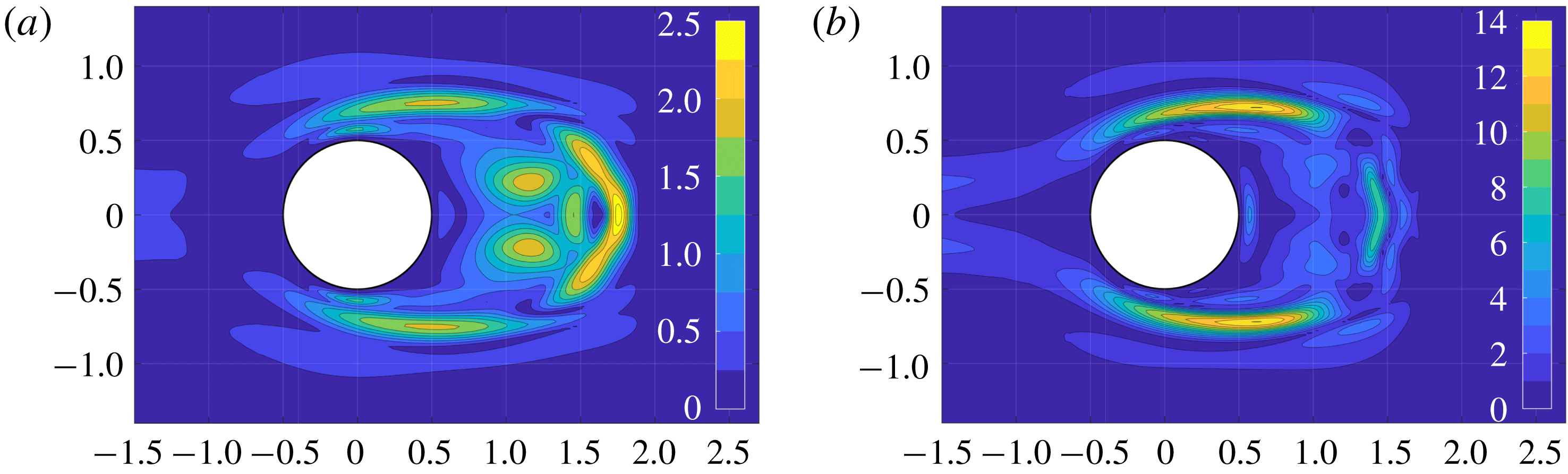
We report in figure 1 the spectral norm of the tensor
 $\unicode[STIX]{x1D64E}_{b}$
obtained for modes A and B and in figure 2 the spectral norm of the tensor
 $\unicode[STIX]{x1D64E}_{l}$
obtained in Giannetti et al. (Reference Giannetti, Camarri and Luchini2010) for the same two configurations. From these figures we note that the region where the spectral norm of
 $\unicode[STIX]{x1D64E}_{b}$
is significantly different from zero is localised in space in a region comprising the shear layers originating on the lateral sides of the cylinder and the recirculation region in the wake. A similar behaviour was observed by Luchini et al. (Reference Luchini, Giannetti and Pralits2009) for the sensitivity of the nonlinearly saturated limit cycle. By comparison between the spatial distribution of
 $\unicode[STIX]{x1D64E}_{b}$
and that of
 $\unicode[STIX]{x1D64E}_{l}$
it is possible to note that the regions in the wake where both are non-negligible are approximately the same; however, differently from
 $\unicode[STIX]{x1D64E}_{l}$
, tensor
 $\unicode[STIX]{x1D64E}_{b}$
is also important on the shear layers in a region extending up to
 $|y|\simeq 1$
. Moreover, in the case of mode B (see figure 1
b),
 $\unicode[STIX]{x1D64E}_{b}$
is significant also upstream of the cylinder at least up to
 $x=-2$
, as also observed for the primary wake instability in Marquet et al. (Reference Marquet, Sipp and Jacquin2008). Figure 3 shows the sum of the spectral norms of
 $\unicode[STIX]{x1D64E}_{b}$
(figure 1) and of
 $\unicode[STIX]{x1D64E}_{l}$
(figure 2) for modes A and B. Despite analysing regions where the spectral norms are non-negligible, it is also interesting to compare tensors
 $\unicode[STIX]{x1D64E}_{b}$
and
 $\unicode[STIX]{x1D64E}_{l}$
from a quantitative viewpoint. This can be done by comparing the values of the spectral norm of
 $\unicode[STIX]{x1D64E}_{b}$
in figure 1 to that of
 $\unicode[STIX]{x1D64E}_{l}$
in figure 2. This comparison shows that for mode A (see panels a) the variation of the Floquet exponent induced by the localised force–velocity feedback due to a change of the base flow, represented by
 $\unicode[STIX]{x1D64E}_{b}$
, is of the same order of magnitude as those induced by the direct action of the perturbation on the dynamics of the 3D perturbations, represented by
 $\unicode[STIX]{x1D64E}_{l}$
. Conversely, as concerns mode B, variations induced by a change of the base flow are dominant, and they are one order of magnitude larger than those related to
 $\unicode[STIX]{x1D64E}_{l}$
. In both cases the contribution of the variations of the base flow is very important and must be taken into account if we want to use the present analysis for a quantitative prediction of possible passive controls of the secondary instability.
Contour plot of the spectral norm of the base flow sensitivity tensor
 $\unicode[STIX]{x1D64E}_{b}$
: (a) mode A (
 $Re=190$
,
 $k=1.585$
) and (b) mode B (
 $Re=260$
,
 $k=7.64$
).
Spatial distribution of the spectral norm of the sensitivity tensor field
 $\unicode[STIX]{x1D64E}_{l}$
, computed and reported in Giannetti et al. (Reference Giannetti, Camarri and Luchini2010): (a) mode A (
 $Re=190$
,
 $k=1.585$
) and (b) mode B (
 $Re=260$
,
 $k=7.64$
).

Field resulting from the sum of the spectral norms of the sensitivity tensor fields
 $\unicode[STIX]{x1D64E}_{b}$
and
 $\unicode[STIX]{x1D64E}_{l}$
: (a) mode A (
 $Re=190$
,
 $k=1.585$
) and (b) mode B (
 $Re=260$
,
 $k=7.64$
).

6.2 Control maps
In this subsection we focus on the idea of providing control maps, derived on the basis of the theoretical work illustrated in § 4 so as to provide quantitative information on the possible control that can be exerted by introducing in the flow a small wire whose axis is parallel to the cylinder axis. An example of this kind of passive control is illustrated in the experiments documented in Zhang et al. (Reference Zhang, Fey and Noack1995). In the referenced experiments, a small wire was observed to interfere with the secondary instability of the wake past a circular cylinder so that, if placed in precise positions, it could stabilise the wake otherwise unstable to 3D instabilities. The diameter of the control wire was in a ratio of 1:160 with the diameter of the circular cylinder.
As a first step, we can model such a localised control as a linear local force–velocity feedback as in (4.10). In particular, following several similar works described in the literature (see for instance Camarri (Reference Camarri2015) for a review), we can model the presence of the small wire as a local pure drag force proportional to the local velocity field. This leads to a tensor field
 $\unicode[STIX]{x1D63E}_{1}$
in (4.9) which is diagonal and equal to
 $\unicode[STIX]{x1D63E}_{1}=-c\,\unicode[STIX]{x1D644}$
, where
 $c$
is a proportionality constant relating the local velocity with the drag and
 $\unicode[STIX]{x1D644}$
is the identity tensor. If we substitute this particular control tensor in (4.10), we obtain the following result quantifying the action of such a control on the Floquet exponent:
 $$\begin{eqnarray}\unicode[STIX]{x1D6FF}\unicode[STIX]{x1D70E}=-c\,\text{Tr}(\unicode[STIX]{x1D64E}_{tot})=-c(\text{Tr}(\unicode[STIX]{x1D64E}_{b})+\text{Tr}(\unicode[STIX]{x1D64E}_{l})).\end{eqnarray}$$
As highlighted in (6.2), the control is proportional by means of
 $-c$
to the trace of the sensitivity tensors
 $\unicode[STIX]{x1D64E}_{b}$
and
 $\unicode[STIX]{x1D64E}_{l}$
, and their sum, which corresponds to
 $\text{Tr}(\unicode[STIX]{x1D64E}_{tot})$
, provides a control map indicating the quantitative action of the local placement of a control wire on the Floquet exponent. In order to analyse the contributions to the control map deriving from the base-flow modifications and from the direct action of the control on the linearised dynamics of the 3D disturbances, we plot both scalar fields
 $\text{Tr}(\unicode[STIX]{x1D64E}_{b})$
and
 $\text{Tr}(\unicode[STIX]{x1D64E}_{l})$
for mode A in figure 4. Confirming what was already observed in § 6.1, the two contributions are equally important for the quantitative evaluation of the control effect. The total control map, which is the sum of the two maps reported in figure 4, is reported in figure 5(a); note that the map is real-valued because the instability mode A remains synchronous with the vortex shedding when the control is applied. The value in the map expresses the quantitative variation
 $\unicode[STIX]{x1D6FF}\unicode[STIX]{x1D70E}/c$
, which in this case is a pure growth rate. The applied control can be stabilising (
 $\unicode[STIX]{x1D6FF}\unicode[STIX]{x1D70E}<0$
) or destabilising (
 $\unicode[STIX]{x1D6FF}\unicode[STIX]{x1D70E}>0$
) depending on the sign of
 $\unicode[STIX]{x1D6FF}\unicode[STIX]{x1D70E}$
. In particular, since
 $c>0$
as the small control wire always exerts a drag, the effect of control is destabilising when the control map in figure 5(a) is positive-valued and destabilising when negative-valued. For example, according to figure 5(a), a control wire positioned at the point
 $(1.05,0.0)$
is stabilising for mode A while a wire in
 $(1.68,0.0)$
is destabilising.
Mode A (
 $Re=190$
,
 $k=1.585$
): scalar fields (a)
 $\text{Tr}(\unicode[STIX]{x1D64E}_{b})$
and (b)
 $\text{Tr}(\unicode[STIX]{x1D64E}_{l})$
.

Analogous comments can be made for the control of mode B. To this purpose we report in figure 6(a) the scalar field
 $\text{Tr}(\unicode[STIX]{x1D64E}_{b})$
, and in figure 6(b)
 $\text{Tr}(\unicode[STIX]{x1D64E}_{l})$
for mode B. In this case, as already highlighted by the sensitivity analysis reported in § 6.1, the contribution of the control to the variation of
 $\unicode[STIX]{x1D6FF}\unicode[STIX]{x1D70E}$
induced by a variation of the base flow can be one order of magnitude larger than that obtained by the direct action on the linearised dynamics. However, this second contribution (derived from
 $\unicode[STIX]{x1D64E}_{l}$
) is important since it is localised in a region where it is of the same order of magnitude as the contribution coming from
 $\unicode[STIX]{x1D64E}_{b}$
. The total control map obtained by the sum of the two contributions is plotted in figure 5(b). As for mode A, mode B is synchronous and it remains synchronous in the controlled case, so that
 $\unicode[STIX]{x1D6FF}\unicode[STIX]{x1D70E}$
is real-valued. If we compare the total control maps for modes A and B, i.e. figures 5(a) and 5(b), it is possible to note that mode B is definitely more sensitive to control. Note, however, that the two maps are pictures taken at two different values of
 $Re$
. Lastly, while control for mode A is equally effective if applied in the shear layers and in the wake, mode B is definitely more sensitive to control if this is applied in the shear layers detaching from the body.
Total control map
 $\text{Tr}(\unicode[STIX]{x1D64E}_{tot})$
: (a) mode A (
 $Re=190$
,
 $k=1.585$
) and (b) mode B (
 $Re=260$
,
 $k=7.640$
).

Mode B (
 $Re=260$
,
 $k=7.640$
): scalar fields (a)
 $\text{Tr}(\unicode[STIX]{x1D64E}_{b})$
and (b)
 $\text{Tr}(\unicode[STIX]{x1D64E}_{l})$
.

Finally, as shown in § 4, a necessary step for the estimation of
 $\unicode[STIX]{x1D6FF}\unicode[STIX]{x1D70E}$
is the evaluation of the control action on the vortex shedding frequency. This estimation, which is implicitly taken into account in (4.10), is an important side output of the analysis for control purposes, as it provides a synthetic control map like those reported in figure 5 illustrating the effect of a control wire generically positioned in the flow on the nonlinearly saturated vortex shedding frequency. In particular, if we model the control wire as proposed above and we substitute the model in (4.2) we obtain
 $$\begin{eqnarray}\unicode[STIX]{x1D6FF}St=-c\,\unicode[STIX]{x1D644}\boldsymbol{ : }\unicode[STIX]{x1D64E}_{s}(x_{0},y_{0})=-c\,\text{Tr}(\unicode[STIX]{x1D64E}_{s})(x_{0},y_{0}).\end{eqnarray}$$
In this case the only contribution to the variation of the vortex shedding is obviously due to the action of the control on the base flow, as indeed vortex shedding is a property of the base flow. The resulting control map, the scalar field
 $\text{Tr}(\unicode[STIX]{x1D64E}_{s})$
, is plotted in figures 7(a) and 7(b) for modes A and B, respectively. Note that, even if it is not immediately clear from the figure, the map comprises also negative values in very localised regions just downstream of the separation points of the shear layers. However, except for these very limited regions, the map is positive-valued, implying a decrease of the vortex shedding frequency or, equivalently, an increase of its period when the control is applied. Moreover, differently from
 $\unicode[STIX]{x1D6FF}\unicode[STIX]{x1D70E}$
, the effect of the control on
 $\unicode[STIX]{x1D6FF}St$
is qualitatively and quantitatively similar for modes A and B, that for mode B being larger by a factor that is roughly equal to
 $1.6$
. In both cases the region where control mostly affects the vortex shedding frequency is localised on the boundaries of the mean recirculation region of the wake. For instance, if we constrain the control wire to be on the symmetry line
 $y=0$
, the position of maximum effect of control for mode A is at
 $x=1.69$
(
 $\unicode[STIX]{x1D6FF}St=6.43\times 10^{-2}\,c$
) and for mode B at
 $x=1.51$
(
 $\unicode[STIX]{x1D6FF}St=9.44\times 10^{-2}\,c$
).
Spatial distribution of the scalar field
 $\text{Tr}(\unicode[STIX]{x1D64E}_{s})$
: (a) mode A (
 $Re=190$
,
 $k=1.585$
) and (b) mode B (
 $Re=260$
,
 $k=7.64$
).

6.3 Validation of the control maps by direct numerical simulation
In this section we provide a validation of the control maps reported and discussed in § 6.2. The validation has been carried out for both modes A and B. Here, for the sake of brevity, we just report results concerning mode A.
We have used the code Nek5000 and 3D simulations whose numerical details are provided in § 5. In order to properly discretise a localised drag force without the need for ad hoc mesh refinements, which might be difficult with a structured grid, and considering that we are using a spectral element method, which may be inaccurate if the forcing applied to the equations is not sufficiently regular, we have chosen to replace the Dirac delta in (4.9) by a more regular but still quite localised function
 $\unicode[STIX]{x1D6FF}_{N}$
in the
 $x{-}y$
planes. In particular, the drag force applied to the momentum equation in the DNS is the following:
 $$\begin{eqnarray}\unicode[STIX]{x1D6FF}\unicode[STIX]{x1D643}_{N}(x,y,z)=-c_{N}\underbrace{\left[\frac{1}{\unicode[STIX]{x03C0}\unicode[STIX]{x1D6FE}^{2}}\exp \left(-\frac{(x-x_{0})^{2}+(y-y_{0})^{2}}{\unicode[STIX]{x1D6FE}^{2}}\right)\right]}_{\unicode[STIX]{x1D6FF}_{N}(\boldsymbol{x}-\boldsymbol{x}_{0})}\boldsymbol{U}(x,y,z),\end{eqnarray}$$
where
 $c_{N}$
is the free proportionality constant of the control and
 $\unicode[STIX]{x1D6FE}$
is a free parameter determining the sharpness of the resulting function
 $\unicode[STIX]{x1D6FF}_{N}$
. Note that the function
 $\unicode[STIX]{x1D6FF}_{N}$
is normalised such that
 $\int _{-\infty }^{\infty }\int _{-\infty }^{\infty }\unicode[STIX]{x1D6FF}_{N}(x,y,x_{0},y_{0})\,\text{d}x\,\text{d}y=1$
. In the simulations documented here, we have fixed
 $\unicode[STIX]{x1D6FE}=0.3$
after having verified that the resulting function
 $\unicode[STIX]{x1D6FF}\unicode[STIX]{x1D643}_{N}$
is represented very well by the numerical discretisation used in the DNS, at least for the considered points
 $(x_{0},y_{0})$
listed in the following. In particular, the numerical integral of
 $\unicode[STIX]{x1D6FF}_{N}$
carried out using the same spectral basis as used for the DNS differs from the exact result by a quantity of the order of
 $10^{-6}$
. For this selected value of
 $\unicode[STIX]{x1D6FE}$
, the force distribution drops to
 $1\,\%$
of its peak at a distance from its application centre equal to
 $0.64~D$
.
Mode A (
 $Re=190$
,
 $k=1.585$
), control point P2. (a) Ratio
 $[(St_{c}-St_{n})/c_{N}]/$
 $(\unicode[STIX]{x1D6FF}St/c_{N})$
, where
 $St_{c}$
and
 $St_{n}$
are the Strouhal numbers of vortex shedding obtained by DNS in the uncontrolled case (
 $St_{n}$
) and using an intensity control equal to
 $c_{N}(St_{c})$
, and
 $\unicode[STIX]{x1D6FF}St/c_{N}$
is the value estimated by (6.6). (b) Ratio
 $[(\unicode[STIX]{x1D70E}_{c}-\unicode[STIX]{x1D70E}_{n})/c_{N}]/(\unicode[STIX]{x1D6FF}\unicode[STIX]{x1D70E}/c_{N})$
, where
 $\unicode[STIX]{x1D70E}_{c}$
and
 $\unicode[STIX]{x1D70E}_{n}$
are the Floquet exponents obtained by DNS in the uncontrolled case (
 $\unicode[STIX]{x1D70E}_{n}$
) and using an intensity control equal to
 $c_{N}(\unicode[STIX]{x1D70E}_{c})$
, and
 $\unicode[STIX]{x1D6FF}\unicode[STIX]{x1D70E}/c_{N}$
is the value estimated by (6.5). The dashed line in both panels is plotted only for simplifying visualisation of the trend given by the points.

When the forcing in (6.4) is substituted in the general equations (4.4) and (4.7), introducing also the sensitivity tensors defined in § 4, we finally obtain the following result for
 $\unicode[STIX]{x1D6FF}\unicode[STIX]{x1D70E}$
:
 $$\begin{eqnarray}\unicode[STIX]{x1D6FF}\unicode[STIX]{x1D70E}=-c_{N}\int _{D}\unicode[STIX]{x1D6FF}_{N}(x-x_{0},y-y_{0})[\unicode[STIX]{x1D64E}_{b}(x,y)+\unicode[STIX]{x1D64E}_{l}(x,y)]\,\text{d}{\mathcal{D}},\end{eqnarray}$$
where the forcing is centred around a selected point
 $(x_{0},y_{0})$
. A similar result is obtained from (4.2) for the variation induced on the Strouhal number:
 $$\begin{eqnarray}\unicode[STIX]{x1D6FF}St=-c_{N}\int _{D}\unicode[STIX]{x1D6FF}_{N}(x-x_{0},y-y_{0})\unicode[STIX]{x1D64E}_{s}(x,y)\,\text{d}{\mathcal{D}}.\end{eqnarray}$$
In the validation proposed here, we have selected a few points which are of interest for the control. For each of them we have computed the estimated values of
 $\unicode[STIX]{x1D6FF}St/c_{N}$
and
 $\unicode[STIX]{x1D6FF}\unicode[STIX]{x1D70E}/c_{N}$
provided by (6.6) and (6.5) and we have compared estimations with the values of the same quantities computed by DNS. The value of
 $c_{N}$
in the DNS simulations is progressively decreased in order to check convergence towards the theoretically estimated values.
On the basis of the experiments in Zhang et al. (Reference Zhang, Fey and Noack1995), one point of interest for the control is point P2, with coordinates
 $(x_{0},y_{0})=(1.05,0.0)$
. The results of the validation test described above, which implies a set of DNS simulations, are reported in figure 8(a,b) for the Strouhal number and the Floquet exponent of mode A, respectively. In particular, in figure 8(a) we plot the ratio between the quantity
 $(St_{c}-St_{n})/c_{N}$
, where
 $St_{c}$
and
 $St_{n}$
are the Strouhal numbers of vortex shedding in the controlled and uncontrolled cases, respectively, computed by DNS using
 $c_{N}$
, and the value
 $\unicode[STIX]{x1D6FF}St/c_{N}$
estimated by (6.6). The ratio must tend approximately to
 $1$
when the value of
 $c_{N}$
is progressively decreased if the provided maps are correct. The limit can be slightly different than
 $1$
since the validation by DNS is carried out with a numerics which is completely different from that used in deriving the control maps. Moreover, variations for very small values of
 $c_{N}$
can be difficult to obtain accurately by DNS. Nevertheless, Figure 8(a), where we report the resulting convergence curve, clearly shows convergence of the results. Moreover, the final number obtained for the lowest value of
 $C_{N}$
(
 $C_{N}=5\times 10^{-3}$
) is equal to
 $1$
to the accuracy of the calculations, indicating an excellent convergence, which validates not only the related control map but also the implementation of the solvers and the numerical resolution used both for the maps and for DNS.
Mode A (
 $Re=190$
,
 $k=1.585$
), control point P1. (a) Ratio
 $[(St_{c}-St_{n})/c_{N}]/$
 $(\unicode[STIX]{x1D6FF}St/c_{N})$
and (b) ratio
 $[(\unicode[STIX]{x1D70E}_{c}-\unicode[STIX]{x1D70E}_{n})/c_{N}]/(\unicode[STIX]{x1D6FF}\unicode[STIX]{x1D70E}/c_{N})$
. For details see the caption of figure 8.

In figure 8(b) we carry out the same analysis but focusing on the ratio between
 $(\unicode[STIX]{x1D70E}_{c}-\unicode[STIX]{x1D70E}_{n})/c_{N}$
, where
 $\unicode[STIX]{x1D70E}_{c}$
and
 $\unicode[STIX]{x1D70E}_{n}$
are the Floquet exponents of mode A in the controlled and uncontrolled case, respectively, computed by DNS using
 $c_{N}$
, and the value
 $\unicode[STIX]{x1D6FF}\unicode[STIX]{x1D70E}/c_{N}$
estimated by (6.5). The reported curves again show clear convergence. Moreover, the final values of
 $\unicode[STIX]{x1D6FF}\unicode[STIX]{x1D70E}/c_{N}$
and
 $\unicode[STIX]{x1D6FF}St/c_{N}$
obtained by DNS and those estimated by the control maps are reported together in table 1, showing that
 $\unicode[STIX]{x1D6FF}St/c_{N}$
is predicted without errors while the discrepancies on
 $\unicode[STIX]{x1D6FF}\unicode[STIX]{x1D70E}/c_{N}$
are of the order of
 $0.3\,\%$
. This last result is plausible since the estimation of
 $\unicode[STIX]{x1D70E}$
by DNS is delicate and in general more difficult than that of the Strouhal number. The control effect has been estimated also for two other points, P1
 $(0.75,0.75)$
and P3
 $(0.00,1.68)$
. In particular, point P1 is not placed on the symmetry axis of the flow. Although it is shown in the literature that an asymmetric forcing may excite a new 3D mode, mode C, it has been verified that, for the low control intensities applied here, mode C is absent. As concerns the effect of a control placed at point P1 on mode A, we report in figure 9 the same convergence curves as shown in figure 8 for point P2. Figure 9 shows convergence between the estimations provided by the control maps and the DNS results as for point P2, with the difference that now convergence curves are not monotonic.
Finally, we report in table 1 the control estimations for the three control points together with the corresponding asymptotic values estimated by DNS. As concerns the control estimations, in table 1 we also split the contributions related to the two sensitivity tensors,
 $\unicode[STIX]{x1D64E}_{b}$
and
 $\unicode[STIX]{x1D64E}_{l}$
, so as to highlight the relative contributions to the final result coming from the modification of the base flow and from the direct action of the control on the perturbation dynamics. As already pointed out, the two contributions for mode A are of the same order of magnitude, and thus both of them must be taken into account for a proper estimation of the effects of control on the instability. Moreover, table 1 also shows that, while the control is stabilising when positioned at points P1 and P2, it is destabilising at P3. In particular, point P3 is interesting because the effect on
 $\unicode[STIX]{x1D6FF}\unicode[STIX]{x1D70E}$
coming from
 $\unicode[STIX]{x1D64E}_{b}$
and
 $\unicode[STIX]{x1D64E}_{l}$
is opposite in sign, i.e. the first is destabilising and the second is stabilising. In the sum of the two, the destabilising contribution coming from
 $\unicode[STIX]{x1D64E}_{b}$
is dominant. This is an example in which a control map solely based on
 $\unicode[STIX]{x1D64E}_{l}$
is not only quantitatively but also qualitatively wrong. As concerns the Strouhal number, controls applied on all points P1, P2 and P3 all lead to a decrease of the vortex shedding frequency.
Mode A (
 $Re=220$
,
 $k=1.585$
), DNS. (a) Instantaneous
 $z$
-component of the velocity field at the point
 $(0.6,0.8,0)$
showing the very stages of development of mode A in the uncontrolled case (dashed line) and in the controlled case when control in (6.4) is applied to points P1, P2 and P3. (b) A zoomed view of panel (a).

Mode A (
 $Re=190$
,
 $k=1.585$
). Effect of the control in (6.4) on
 $\unicode[STIX]{x1D6FF}\unicode[STIX]{x1D70E}$
, separating the two contributions coming from
 $\unicode[STIX]{x1D64E}_{b}$
and
 $\unicode[STIX]{x1D64E}_{l}$
, and on
 $\unicode[STIX]{x1D6FF}St$
, for three different points of application of the control. Values estimated by DNS are also reported for validation.

As an overall qualitative and comparative inspection of the effect of the mentioned controls, they have been applied to the flow at
 $Re=220$
starting from the same initial conditions, in which mode A is at the very first stage of development. A slightly larger value of
 $Re$
instead of
 $Re=190$
has been chosen in order to have larger growth factors for mode A, thus simplifying the DNS analysis of the behaviour of the three different controls. The intensity of the control applied in the DNS is
 $c_{N}=2.5\times 10^{-3}$
, which is sufficiently small so that the control maps provide a reasonable estimation of its effect and, at the same time, it is sufficiently strong to highlight the effect of the control by a visual inspection of the results (see figure 10). We remind the reader that the control applied in this test is intentionally not enough strong to stabilise the flow when applied at P1 or at P2 (P3 is a destabilising position) since the objective of the test is only to put in evidence qualitatively the comparative effect of a slight control when applied in the three different positions considered. The resulting
 $z$
-component of the velocity on a point in the wake (coordinates
 $(0.6,0.8,0)$
) is reported together with the uncontrolled case (dashed line) in figure 10. Inspecting figure 10(b) and the zoomed view reported in figure 10(b), it is possible to verify that control at P3 is destabilising, while at P1 and P2 it is stabilising. Moreover, as predicted by the maps, control at P2 is more stabilising than that at P1. Finally, in all cases the period of vortex shedding increases with respect to the uncontrolled one, the effect being less important when control is applied on P2.
6.4 Estimating experimental results in Zhang et al. (Reference Zhang, Fey and Noack1995) by control maps
In this section we provide a partial validation of the control maps derived in § 6.2 by comparing their estimations against the experimental results in Zhang et al. (Reference Zhang, Fey and Noack1995), where passive control of the secondary instability is attempted by placing a small wire in the wake past a circular cylinder. In the experiments, the cylinder generating the wake has a diameter equal to
 $D=4~\text{mm}$
while the control wire is significantly smaller, with a diameter
 $d$
equal to
 $d=25~\unicode[STIX]{x03BC}\text{m}$
(
 $D/d=160.0$
). Experiments show that the control wire, placed in proper positions, can suppress the 3D instability of the wake leading the flow to a 2D regime even at supercritical values of the flow Reynolds numbers. In particular, we consider two cases. In the first one the wire is placed at point P2
 $(1.05,0)$
and in the second one at point P1 (already defined in § 6.3, the coordinates being
 $(0.75,0.75)$
). When the wire is at position P2, instability is suppressed at
 $Re=219$
and starts again when
 $Re\geqslant 230$
. When the wire is at point P1, the flow remains 2D for
 $Re=260$
and becomes 3D at
 $Re=270$
.
The control maps provided in § 6.2 can be used to predict the two experimental cases described above. To this purpose it is necessary to estimate, for each case, the Floquet exponent in the uncontrolled case and its variation due to the control. This information allows one to predict a possible stabilisation of the instability and to compare with the experimental evidence. In order to estimate the effect of control on the basis of the control maps, it is necessary to model the action that the control wire exerts on the flow as a pointwise linear force–velocity feedback. Focusing for the moment on the first experimental case (point P2,
 $Re=219$
), we have simulated the velocity field at
 $Re=220$
when the flow is 2D and we have extracted the velocity at the point where the control wire is positioned in the experiments. The velocity at that point is periodic in time due to vortex shedding and its maximum norm is approximately equal to
 $0.79U_{\infty }$
, which corresponds to a maximum local Reynolds number, based on the wire diameter
 $d$
and on the local velocity, equal to
 $Re_{d,max}\simeq 1.08$
. The diameter of the control wire is definitely smaller than the local inhomogeneity characteristic length of the flow, which scales with
 $D$
, and thus it is possible to assume that the force exerted by the control wire on the flow is a pure drag which depends on the local flow conditions. Moreover, the advection time scale near the control wire is much smaller than the vortex shedding period, thus we can assume that the drag of the control wire adjusts instantaneously to the local flow conditions with negligible inertial effects (quasi-static assumption). Assuming a quasi-static behaviour of the drag exerted by the flow on the control wire and considering the value of
 $Re_{d,max}$
, we use Lamb’s law (see e.g. Landau & Lifshitz Reference Landau and Lifshitz1987) for the estimation of the drag coefficient, which, once normalised with
 $d$
and with the local velocity norm, is given by the following equation:
 $$\begin{eqnarray}C_{d,wire}(Re_{d})=\frac{8\unicode[STIX]{x03C0}}{Re_{d}}\left(\log \frac{8}{Re_{d}}-\unicode[STIX]{x1D6FE}+\frac{1}{2}\right)^{-1},\end{eqnarray}$$
where
 $\unicode[STIX]{x1D6FE}$
is the Euler constant (
 $\unicode[STIX]{x1D6FE}\simeq 0.577216$
). The same approximation for a similar control application has been followed for instance in Meliga et al. (Reference Meliga, Boujo, Pujals and Gallaire2014, Reference Meliga, Boujo and Gallaire2016). The Cartesian components of the resulting force in one shedding period are computed using the local velocity history simulated at point P2 and the Lamb law in (6.7) and, once normalised using
 $U_{\infty }$
and
 $D$
, are reported in figure 11 with a continuous line. In order to straightforwardly use the control maps proposed in § 6.2, the forces reported in figure 11 are approximated by a linear force–velocity feedback. To this purpose the coefficient of proportionality
 $c$
in (6.2) is tuned so as to fit the true forces reported in figure 11 in a least-squares sense. The resulting value,
 $c\simeq 2.68\times 10^{-2}$
, leads to the estimated force components plotted as a dashed line in figure 11. By the comparison between the true (continuous) and the approximate force (dashed) lines, it is possible to see that the fit provided by the tuned linear model can be considered satisfactory. Once the constant
 $c$
has been estimated, by multiplying its value with the value of the control map at the point P2 (see figure 5
a), as indicated in (6.2), we obtain the estimated variation of the Floquet exponent due to control, which in this case is equal to
 $\unicode[STIX]{x1D6FF}\unicode[STIX]{x1D70E}=-0.057$
. The value of the Floquet exponent at
 $Re=220$
in the uncontrolled case has been computed by DNS and it is equal to
 $\unicode[STIX]{x1D70E}_{220}=0.047$
. The resulting controlled Floquet exponent is thus negative, i.e.
 $\unicode[STIX]{x1D70E}_{220}+\unicode[STIX]{x1D6FF}\unicode[STIX]{x1D70E}<0$
. This means that the control map, used in the way detailed above, predicts a stabilisation of the flow for
 $Re=220$
when the wire is positioned at P2, in agreement with the experiments in Zhang et al. (Reference Zhang, Fey and Noack1995). Repeating the same procedure for
 $Re=230$
we find that
 $\unicode[STIX]{x1D70E}_{230}+\unicode[STIX]{x1D6FF}\unicode[STIX]{x1D70E}>0$
, where
 $\unicode[STIX]{x1D70E}_{230}=0.0625$
is again estimated by DNS and
 $\unicode[STIX]{x1D6FF}\unicode[STIX]{x1D70E}$
is approximately the same as that evaluated at
 $Re=220$
. Thus, according to the control maps, the wire does not stabilise the 3D wake instability in this case, and this is again in agreement with the experiments. Note that in the calculations detailed above we have assumed for simplicity that the control map for mode A at
 $Re=220$
is not significantly different from that at
 $Re=190$
reported in figure 5(a), thus avoiding the need to recompute a new control map. This assumption has been verified by DNS, showing that quantitative variation of the control map at point P2 for mode A at
 $Re=220$
is of the order of
 $15\,\%$
with respect to the case at
 $Re=190$
, which makes our approximation acceptable considering the type of comparison that we are carrying out with the experiments and the type of information we can extract from Zhang et al. (Reference Zhang, Fey and Noack1995). In this respect we also recall that the analysis carried out here is the result of a linearisation of the problem, which is inherently nonlinear, around the uncontrolled flow state.
Cartesian components of the force acting on the control wire at
 $Re=220$
: quasi-static model based on Lamb’s equation in continuous lines and tuned linear model in dashed lines.
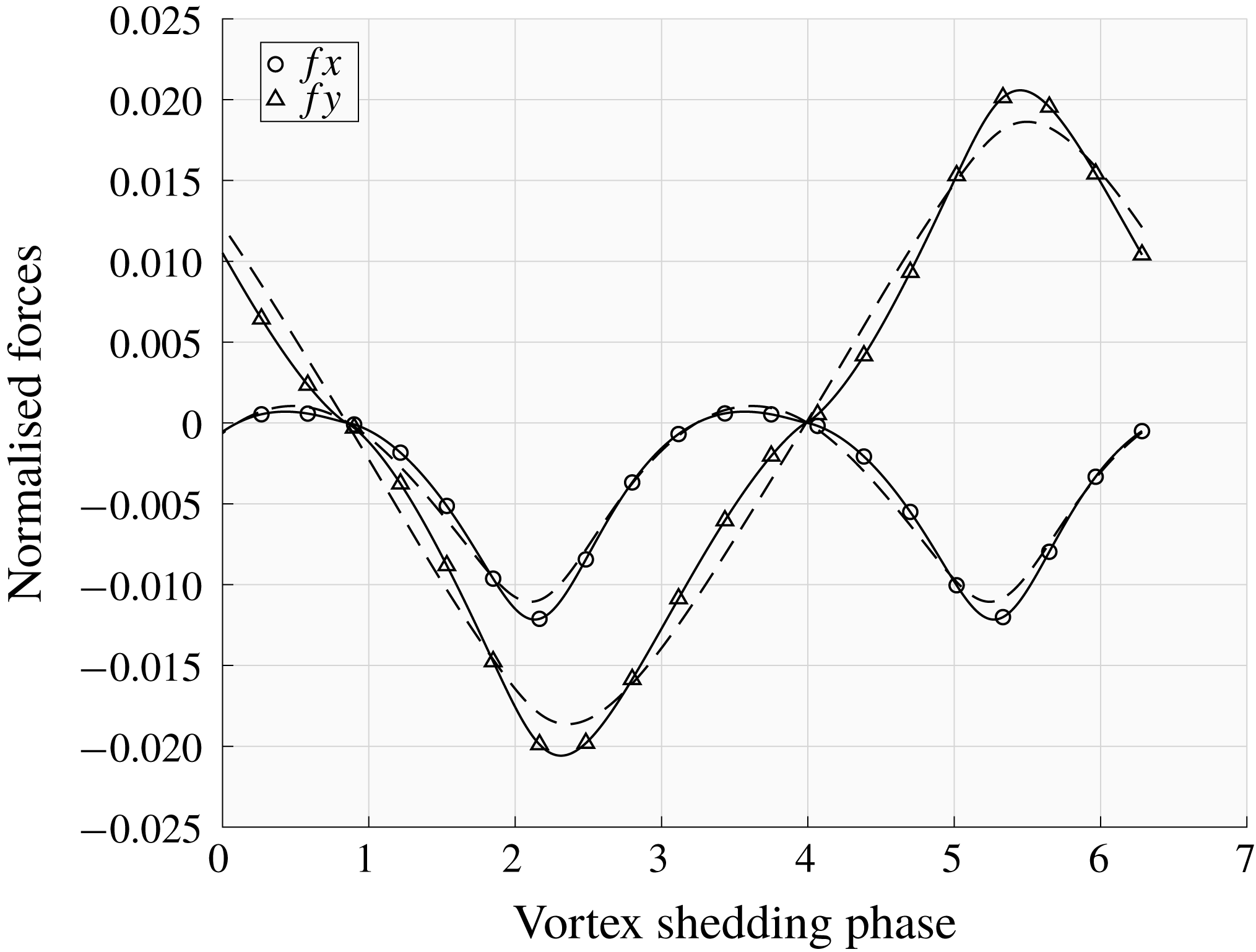
The procedure illustrated above has been repeated for the second experimental case, i.e. when the control wire is positioned at point P1. In this case we can estimate on the basis of the control maps that a wire of the same size as that used in the experiments leads to
 $\unicode[STIX]{x1D6FF}\unicode[STIX]{x1D70E}=-0.0845$
in the controlled case. Since
 $\unicode[STIX]{x1D70E}_{230}=0.0625$
we can deduce that the flow is stabilised, according to our theoretical estimation since
 $\unicode[STIX]{x1D70E}_{230}+\unicode[STIX]{x1D6FF}\unicode[STIX]{x1D70E}<0$
. Moreover, considering that the Floquet exponent for
 $Re=260$
is approximately equal to
 $\unicode[STIX]{x1D70E}_{260}=0.0910$
and assuming a linear variation of
 $\unicode[STIX]{x1D70E}$
with
 $Re$
in the range
 $230\leqslant Re\leqslant 260$
, we can deduce, again on the basis of the control maps, that the wire at position P1 leads to a stabilisation of mode A up to
 $Re\simeq 254$
, which is in fairly good agreement with Zhang et al. (Reference Zhang, Fey and Noack1995), where it is shown that stabilisation is active up to
 $Re=260$
.
7 Conclusions
In this paper we have presented a general theoretical methodology for conducting sensitivity analysis with respect to a generic forcing acting on the base flow for cases in which the base flow is periodic in time. Differently from the analysis considered previously by Giannetti et al. (Reference Giannetti, Camarri and Luchini2010), where the effects of a perturbation acting solely on the disturbance equations is investigated, we now study the sensitivity of the Floquet exponent when a structural perturbation is acting on the base-flow equations. The effect of such a perturbation is able to generate a change of the base flow which, in turn, affects the stability equations through a change of the coefficients of the linearised Navier–Stokes operator. Here we derive the expression of the sensitivity tensor for the Floquet exponent of a given instability and for the frequency of the saturated limit cycle of the base flow with respect to a generic forcing of the base flow itself. In this respect the present work and that in Giannetti et al. (Reference Giannetti, Camarri and Luchini2010) can be considered an extension of the seminal work by Marquet et al. (Reference Marquet, Sipp and Jacquin2008) and Luchini et al. (Reference Luchini, Giannetti and Pralits2009) to the case of base flows which are periodic in time.
Although the theory proposed here is general, it has been particularised since the beginning so as to study the second bifurcation of the flow past a circular cylinder. Sensitivity results for two nearly marginally unstable flow conditions are discussed: Reynolds number
 $Re=190$
is selected to study mode A while
 $Re=260$
is adopted to investigate mode B.
Firstly we started to discuss the differences between the spectral norm of the structural sensitivity tensors computed in Giannetti et al. (Reference Giannetti, Camarri and Luchini2010) and of the tensors representing the sensitivity to a base-flow variation, which are derived here for the first time. The resulting sensitivity maps are highly localised in the flow region immediately past the bluff body. The control maps derived on the basis of the sensitivity tensors have been validated here using dedicated 3D DNS simulations.
The analysis presented is successively used to estimate the control on the 3D instability that might be obtained by placing a small wire in the flow. Assuming that the control wire experiences a quasi-static drag force, we can build control maps predicting the variation of the vortex shedding frequency and of the Floquet exponent for a given instability mode (A or B) versus a generic position of the wire. Besides being interesting by itself, this kind of control has already been applied in the experiments carried out by Zhang et al. (Reference Zhang, Fey and Noack1995). It is shown here that the quantitative agreement between the experiments in Zhang et al. (Reference Zhang, Fey and Noack1995) and the proposed theory is definitely satisfactory.
Summarising, there are two main outputs of the present work. On one side, we propose a general theory for the design of passive controls of instabilities developing on time-periodic base flows. On the other side, by applying this methodology, we provide original results on a classical but still actively studied problem in the literature, which is the secondary instability of the wake past a circular cylinder.
Acknowledgements
The authors wish to thank the CINECA Computing Center (Bologna, Italy) for allowance of computational time under the ISCRA programme.



