2 Formulation

The physical configuration is that sketched in figure 2. The flow is taken to be contained between the inner and outer cylinders depicted there. The inner cylinder has a radius $R_{i}$ and the outer cylinder has a radius $R_{o}$ . The origin of the stationary $x^{\prime }{-}y^{\prime }$ coordinate system is located at the centre of the inner cylinder. The centre of the outer cylinder is located at $x^{\prime }=-e,y^{\prime }=0$ . The inner cylinder rotates at a constant rate $\unicode[STIX]{x1D714}$ while the outer cylinder is stationary. For convenience, we refer to the inner cylinder as the rotor and the outer cylinder as the stator.

Figure 2.

Sketch of physical configuration.

Figure 3.

Unwrapped configuration. The stationary outer cylinder of figure 2 is approximated by the $y=h(x)$ surface and the rotating inner cylinder is approximated by the $y=0$ surface. The minimum gap width is $h_{o}\equiv h(0)$ and the maximum value of $h(x)$ is $h_{m}\equiv h(L/2)$ .

Throughout this work we apply the thin film approximation so that we compute the flow details using the ‘unwrapped’ configuration sketched in figure 3. When $R_{o}\approx R_{i}$ the fluid can be taken to be contained in the region $0\leqslant y\leqslant h(x)$ , where the variable $y$ is recognized as a distance measured normal to the inner cylinder and $x\equiv \unicode[STIX]{x1D703}R_{i}$ is distance measured along the inner cylinder. The curve $y=h(x)$ in figure 3 approximately corresponds to the surface of the stator. We can now define $L\equiv 2\unicode[STIX]{x03C0}R_{i}$ which is just the circumference of the inner cylinder and $h_{o}\equiv h(0)$ which is the minimum gap width; we take $h_{o}$ to be a measure of the film thickness. For the non-concentric cylinders sketched in figure 2, the thickness of the fluid layer can be approximated by

(2.1) $$\begin{eqnarray}\overline{h}\equiv \frac{h(x)}{h_{o}}\approx 1+\unicode[STIX]{x1D6FF}-\unicode[STIX]{x1D6FF}\cos (\unicode[STIX]{x1D703}),\end{eqnarray}$$

where

(2.2) $$\begin{eqnarray}\unicode[STIX]{x1D6FF}\equiv \frac{1}{2}(\overline{h}_{m}-1)=\frac{\unicode[STIX]{x1D716}}{1-\unicode[STIX]{x1D716}}.\end{eqnarray}$$

The quantity $\overline{h}_{m}\equiv \overline{h}(\overline{x}=1/2)=\overline{h}(\unicode[STIX]{x1D703}=\unicode[STIX]{x03C0})$ is the maximum value of $\overline{h}$ . The factor $\unicode[STIX]{x1D6FF}$ has been related to the eccentricity ratio $\unicode[STIX]{x1D716}\equiv e/c$ where $c\equiv R_{o}-R_{i}$ is called the radial clearance; the eccentricity $\unicode[STIX]{x1D716}$ is commonly used in the lubrication literature; see, e.g. Pinkus & Sternlicht (Reference Pinkus and Sternlicht1961), Gross et al. (Reference Gross, Matsch, Castelli, Eshel, Vohr and Wildmann1980), Hamrock et al. (Reference Hamrock, Schmidt and Jacobson2004) or Szeri (Reference Szeri2010).

In our detailed calculations we will employ (2.1). However, many of our results are also valid under the weaker condition that $\overline{h}$ be symmetric about $\unicode[STIX]{x1D703}=\unicode[STIX]{x03C0}$ , i.e.

(2.3) $$\begin{eqnarray}\overline{h}(\unicode[STIX]{x03C0}-\unicode[STIX]{x1D703})\equiv \overline{h}(\unicode[STIX]{x1D703}-\unicode[STIX]{x03C0}).\end{eqnarray}$$

As a result, the derivatives of $\overline{h}$ ( $\unicode[STIX]{x1D703}$ ) will satisfy

(2.4) $$\begin{eqnarray}\frac{\text{d}\overline{h}}{\text{d}\unicode[STIX]{x1D703}}(\unicode[STIX]{x03C0}-\unicode[STIX]{x1D703})=-\frac{\text{d}\overline{h}}{\text{d}\unicode[STIX]{x1D703}}(-(\unicode[STIX]{x03C0}-\unicode[STIX]{x1D703})).\end{eqnarray}$$

In order to ensure that $\overline{h}$ is a minimum at $\overline{x}=0$ , 1 or $\unicode[STIX]{x1D703}=0,2\unicode[STIX]{x03C0}$ , we require that

(2.5) $$\begin{eqnarray}\displaystyle \frac{\text{d}\overline{h}}{\text{d}\unicode[STIX]{x1D703}} & {\geqslant} & \displaystyle 0\text{ if }0\leqslant \unicode[STIX]{x1D703}\leqslant \unicode[STIX]{x03C0}\nonumber\\ \displaystyle & {\leqslant} & \displaystyle 0\text{if }\unicode[STIX]{x03C0}\leqslant \unicode[STIX]{x1D703}\leqslant 2\unicode[STIX]{x03C0}.\end{eqnarray}$$

The flow will be taken to be steady, two-dimensional, compressible, single phase and laminar. The physical flow is required to satisfy the usual thin film and lubrication restrictions, i.e.

(2.6) $$\begin{eqnarray}\displaystyle & \displaystyle \frac{h_{o}}{L}\ll 1, & \displaystyle\end{eqnarray}$$

(2.7) $$\begin{eqnarray}\displaystyle & \displaystyle Re\frac{h_{o}^{2}}{L^{2}}\ll 1, & \displaystyle\end{eqnarray}$$

where $Re$ is the Reynolds number based on $L$ , $U\equiv R_{i}\unicode[STIX]{x1D714}$ , $\unicode[STIX]{x1D707}_{ref}$ and $\unicode[STIX]{x1D70C}_{ref}$ . The subscript ‘ref’ will always refer to quantities evaluated at a given reference thermodynamic state. Here we take that reference state to be that at $x=0$ and $L$ . As discussed by Chien et al. (Reference Chien, Cramer and Untaroiu2017a ) we also need to require that the flow be sufficiently far from the thermodynamic critical point. If the rotor and stator are both isothermal, we must also require that the product of the fixed, known temperature difference and the thermal expansion coefficient defined by (A 6) be small. Under these conditions, the flow will satisfy the Reynolds equation of Chien et al. (Reference Chien, Cramer and Untaroiu2017a ) which can be written in non-dimensional form as

(2.8) $$\begin{eqnarray}\frac{\text{d}}{\text{d}\overline{x}}\bigg(\overline{h}^{3}\overline{\unicode[STIX]{x1D705}}_{Te}\frac{\text{d}\overline{\unicode[STIX]{x1D70C}}}{\text{d}\overline{x}}\bigg)=\unicode[STIX]{x1D6EC}\frac{\text{d}(\overline{\unicode[STIX]{x1D70C}}\overline{h})}{\text{d}\overline{x}},\end{eqnarray}$$

where $\overline{\unicode[STIX]{x1D70C}}\equiv \unicode[STIX]{x1D70C}/\unicode[STIX]{x1D70C}_{ref}$ is the non-dimensional density. Here $\overline{x}\equiv x/L$ and

(2.9) $$\begin{eqnarray}\overline{\unicode[STIX]{x1D705}}_{Te}=\overline{\unicode[STIX]{x1D705}}_{Te}(\overline{\unicode[STIX]{x1D70C}})\equiv \frac{\unicode[STIX]{x1D705}_{Te}(\unicode[STIX]{x1D70C},T_{ref})}{\unicode[STIX]{x1D705}_{Te}|_{ref}}=\frac{\unicode[STIX]{x1D705}_{Te}(\unicode[STIX]{x1D70C},T_{ref})}{\unicode[STIX]{x1D705}_{Te}(\unicode[STIX]{x1D70C}_{ref},T_{ref})}\end{eqnarray}$$

is the scaled effective bulk modulus. For the present purposes, the Reynolds equation (2.8) will be integrated subject to the periodicity conditions

(2.10) $$\begin{eqnarray}\overline{\unicode[STIX]{x1D70C}}(0)=\overline{\unicode[STIX]{x1D70C}}(1)=1.\end{eqnarray}$$

The solution for the fluid density is generally obtained by integrating (2.8) subject to (2.10) to yield $\overline{\unicode[STIX]{x1D70C}}=\overline{\unicode[STIX]{x1D70C}}$ ( $\overline{x}$ ; $\unicode[STIX]{x1D6EC}$ ) once the reference thermodynamic state ( $\unicode[STIX]{x1D70C}_{ref}$ , $T_{ref}$ ) and gas models are specified. The pressure is then found by substitution in the equation of state.

In the following discussion, a convenient first integral of (2.8) is

(2.11) $$\begin{eqnarray}\overline{\unicode[STIX]{x1D70C}}=\frac{1}{\overline{h}}+\frac{1}{\unicode[STIX]{x1D6EC}}\bigg(\overline{h}^{2}\overline{\unicode[STIX]{x1D705}}_{Te}\frac{\text{d}\overline{\unicode[STIX]{x1D70C}}}{\text{d}\overline{x}}-\frac{1}{\overline{h}}\frac{\text{d}\overline{\unicode[STIX]{x1D70C}}}{\text{d}\overline{x}}(0)\bigg),\end{eqnarray}$$

where we have used the fact that $\overline{h}=\overline{\unicode[STIX]{x1D705}}_{Te}=1$ at $\overline{x}=0$ . In the limit of incompressible flow with constant viscosity (2.11) reduces to Reynolds’ original formula (1.1) with

(2.12) $$\begin{eqnarray}\frac{\text{d}\overline{\unicode[STIX]{x1D70C}}}{\text{d}\overline{x}}(0)\end{eqnarray}$$

playing the role of the integration constant.

With the thin film approximation (2.6) we can write the $x^{\prime }$ and $y^{\prime }$ components of the forces on the rotor from the fluid as

(2.13) $$\begin{eqnarray}\displaystyle & \displaystyle \overline{F}_{x^{\prime }}\approx \int _{0}^{2\unicode[STIX]{x03C0}}\overline{p}\cos (\unicode[STIX]{x1D703})\,\text{d}\unicode[STIX]{x1D703}=-\frac{1}{2\unicode[STIX]{x03C0}}\int _{0}^{2\unicode[STIX]{x03C0}}\frac{\text{d}\overline{p}}{\text{d}\overline{x}}\text{sin}(\unicode[STIX]{x1D703})\,\text{d}\unicode[STIX]{x1D703}, & \displaystyle\end{eqnarray}$$

(2.14) $$\begin{eqnarray}\displaystyle & \displaystyle \overline{F}_{y^{\prime }}\approx \int _{0}^{2\unicode[STIX]{x03C0}}\overline{p}\text{sin}(\unicode[STIX]{x1D703})\,\text{d}\unicode[STIX]{x1D703}=\frac{1}{2\unicode[STIX]{x03C0}}\int _{0}^{2\unicode[STIX]{x03C0}}\frac{\text{d}\overline{p}}{\text{d}\overline{x}}\cos (\unicode[STIX]{x1D703})\,\text{d}\unicode[STIX]{x1D703}, & \displaystyle\end{eqnarray}$$

where

(2.15) $$\begin{eqnarray}\overline{\boldsymbol{F}}\equiv -\frac{h_{o}^{2}}{\unicode[STIX]{x1D707}_{ref}U2\unicode[STIX]{x03C0}R_{i}^{2}b}\boldsymbol{F}^{\prime },\end{eqnarray}$$

$b$ is the length of the cylinders in the $z^{\prime }$ -direction, and $\boldsymbol{F}^{\prime }$ is the dimensional force on the rotor. The quantity $\overline{p}$ is the scaled pressure and is related to the dimensional pressure $p$ by

(2.16) $$\begin{eqnarray}\overline{p}\equiv \frac{h_{o}^{2}}{\unicode[STIX]{x1D707}_{ref}UL}(p-p_{ref}).\end{eqnarray}$$

The power loss is the work per time done on the rotor, i.e. the $y=0$ surface in figure 3. In the thin film approximation, this can be written

(2.17) $$\begin{eqnarray}P=bU\int _{0}^{L}T_{yx}\,\text{d}x\approx \frac{bLU^{2}\unicode[STIX]{x1D707}_{ref}}{h_{o}}\overline{P},\end{eqnarray}$$

where the scaled loss is

(2.18) $$\begin{eqnarray}\overline{P}\equiv \int _{0}^{1}\bigg(\overline{\unicode[STIX]{x1D707}}\frac{\unicode[STIX]{x2202}u}{\unicode[STIX]{x2202}\overline{y}}\bigg)\bigg|_{\overline{y}=0}\,\text{d}\overline{x},\end{eqnarray}$$

$\overline{\unicode[STIX]{x1D707}}\equiv$ $\unicode[STIX]{x1D707}/\unicode[STIX]{x1D707}_{ref}$ is a scaled version of the viscosity, and $\overline{y}\equiv y/h_{o}$ is the scaled $y$ -coordinate. The $x$ -component of the fluid velocity, denoted by $u$ , is scaled with $U$ and its expression is given in appendix A.

3 General results

We now determine the approximate solutions to the Reynolds equation (2.8) for lubrication flows with large speed numbers. We first consider the second-order expansion for density, i.e.

(3.1) $$\begin{eqnarray}\overline{\unicode[STIX]{x1D70C}}=\unicode[STIX]{x1D70C}_{0}+\frac{\unicode[STIX]{x1D70C}_{1}}{\unicode[STIX]{x1D6EC}}+\frac{\unicode[STIX]{x1D70C}_{2}}{\unicode[STIX]{x1D6EC}^{2}}+O\left(\frac{1}{\unicode[STIX]{x1D6EC}^{3}}\right).\end{eqnarray}$$

If we substitute (3.1) and its derivative in (2.11), we then obtain the functions

(3.2) $$\begin{eqnarray}\displaystyle & \displaystyle \unicode[STIX]{x1D70C}_{0}=\frac{1}{\overline{h}}, & \displaystyle\end{eqnarray}$$

(3.3) $$\begin{eqnarray}\displaystyle & \displaystyle \unicode[STIX]{x1D70C}_{1}=-\overline{\unicode[STIX]{x1D705}}_{Teo}\frac{\text{d}\overline{h}}{\text{d}\overline{x}}, & \displaystyle\end{eqnarray}$$

(3.4) $$\begin{eqnarray}\displaystyle & \displaystyle \unicode[STIX]{x1D70C}_{2}=-\overline{h}^{2}\frac{\text{d}}{\text{d}\overline{x}}\left(\overline{\unicode[STIX]{x1D705}}_{Te}^{2}\frac{\text{d}\overline{h}}{\text{d}\overline{x}}\right)\bigg|_{o}+\frac{1}{\overline{h}}\frac{\text{d}^{2}\overline{h}}{\text{d}\overline{x}^{2}}(0), & \displaystyle\end{eqnarray}$$

where the subscript ‘o’ will always refer to quantities evaluated at the lowest-order density, $\overline{\unicode[STIX]{x1D70C}}\approx 1/\overline{h}$ . For example,

(3.5) $$\begin{eqnarray}\overline{\unicode[STIX]{x1D705}}_{Teo}(\overline{\unicode[STIX]{x1D70C}})\equiv \overline{\unicode[STIX]{x1D705}}_{Te}\left(\frac{1}{\overline{h}}\right).\end{eqnarray}$$

It is easily verified that (3.1)–(3.4) satisfy the boundary conditions (2.10) and the equation for $\overline{h}$ , i.e. (2.1), to the appropriate order.

Figure 4.

Scaled density versus $x/L$ at $V(0)=V(L)=10V_{c}$ , $T(0)=T(L)=1.05T_{c}$ , $\unicode[STIX]{x1D6FF}=0.5$ , $\unicode[STIX]{x1D6EC}=40$ . The symbols ○ denote the exact solutions to the Reynolds equation (2.8). The solid line denotes the lowest-order solutions, i.e. $\overline{\unicode[STIX]{x1D70C}}=1/\overline{h}$ . The dashed and dash-dot lines represent the first- and second-order solutions of the scaled density (3.1), respectively.

Figure 5.

Scaled density versus $x/L$ at $V(0)=V(L)=2V_{c}$ , $T(0)=T(L)=1.05T_{c}$ , $\unicode[STIX]{x1D6FF}=0.5,\unicode[STIX]{x1D6EC}=40$ . The symbols ○ denote the exact solutions to the Reynolds equation (2.8). The solid line denotes the lowest-order solutions, i.e. $\overline{\unicode[STIX]{x1D70C}}=1/\overline{h}$ . The dashed and dash-dot lines represent the first- and second-order solutions of the scaled density (3.1), respectively.

To demonstrate the accuracy of (3.1)–(3.4), we have plotted a comparison of the approximate density (3.1) and the numerical solution to the exact Reynolds equation (2.8) at $\unicode[STIX]{x1D6EC}=40$ in figures 4–5. Here we take the channel sketched in figure 3 to be given by $h_{o}/L=1.989\times 10^{-5}$ , and $\unicode[STIX]{x1D6FF}=0.5$ . The gas models are taken to be those described in § 4. The temperature at the entrance and exit is taken to be $T(0)=T(L)=1.05T_{c}$ . In figure 4 the specific volume, i.e. $V\equiv 1/\unicode[STIX]{x1D70C}$ , is taken to satisfy $V(0)=V(L)=10V_{c}$ . The pressure at this state is approximately 21.2 bar ${\approx}0.29p_{c}$ , so that the thermodynamic state can be regarded as that of a dense gas. In figure 5 we consider the case of a slightly supercritical fluid in which the reference specific volume is taken to be $V(0)=V(L)=2V_{c}$ and the corresponding pressure is approximately 78.2 bar ${\approx}1.06p_{c}$ .

Inspection of figures 4 and 5 reveals that the second-order approximation is in excellent agreement with the exact solutions. As compared to the lowest-order approximation, the first-order term corrects the slope of the curves near both ends of the channel whereas the second-order correction term further improves the prediction of the position and magnitude of the local minimum.

The accuracy of our approximation for both cases increases as $\unicode[STIX]{x1D6EC}\longrightarrow \infty$ . In order to illustrate the accuracy of the approximation, we have also plotted the root-mean-square error (RMSE) between the approximate density (3.1) and the exact solution to the Reynolds equation (2.8) as a function of $\unicode[STIX]{x1D6EC}$ in figure 6. It was found that the second-order approximation can provide reasonable accuracy when $\unicode[STIX]{x1D6EC}\geqslant$ 20. When $\unicode[STIX]{x1D6EC}=20$ , the RMSEs of the second-order approximation for cases of $V(0)=V(L)=10V_{c}$ and $2V_{c}$ are approximately 1.4 % and 8 %, respectively.

Figure 6.

Root-mean-square error (RMSE) between the approximate and exact density versus $\unicode[STIX]{x1D6EC}$ at $T(0)=T(L)=1.05T_{c}$ and $\unicode[STIX]{x1D6FF}=0.5$ . The symbols ▪, ● and ▾ represent the lowest-, first- and second-order approximations, respectively, at $V(0)=V(L)=2V_{c}$ . The symbols ▫, ○ and ▿ represent the lowest-, first- and second-order approximations, respectively, at $V(0)=V(L)=10V_{c}$ .

We now turn to the determination of the large $\unicode[STIX]{x1D6EC}$ approximation for the forces, i.e. (2.13) and (2.14), on the rotor. If we use (1.3), (1.4) and (2.16), the expressions for the exact force components (2.13) and (2.14) can be rewritten as

(3.6) $$\begin{eqnarray}\displaystyle -\frac{\unicode[STIX]{x1D6EC}}{6}\overline{F}_{x^{\prime }} & = & \displaystyle \frac{1}{2\unicode[STIX]{x03C0}}\int _{0}^{2\unicode[STIX]{x03C0}}\mathscr{R}\frac{\text{d}\overline{\unicode[STIX]{x1D70C}}}{\text{d}\overline{x}}\text{sin}(\unicode[STIX]{x1D703})\,\text{d}\unicode[STIX]{x1D703},\end{eqnarray}$$

(3.7) $$\begin{eqnarray}\displaystyle \frac{\unicode[STIX]{x1D6EC}}{6}\overline{F}_{y^{\prime }} & = & \displaystyle \frac{1}{2\unicode[STIX]{x03C0}}\int _{0}^{2\unicode[STIX]{x03C0}}\mathscr{R}\frac{\text{d}\overline{\unicode[STIX]{x1D70C}}}{\text{d}\overline{x}}\cos (\unicode[STIX]{x1D703})\,\text{d}\unicode[STIX]{x1D703},\end{eqnarray}$$

where the factor

(3.8) $$\begin{eqnarray}\mathscr{R}=\mathscr{R}(\overline{\unicode[STIX]{x1D70C}},T_{ref})\equiv \frac{\overline{\unicode[STIX]{x1D705}}_{T}}{\overline{\unicode[STIX]{x1D70C}}},\end{eqnarray}$$

can be expanded in a Taylor series for $\overline{\unicode[STIX]{x1D70C}}$ near 1/ $\overline{h}$ yielding

(3.9) $$\begin{eqnarray}\mathscr{R}(\overline{\unicode[STIX]{x1D70C}},T_{ref})=\mathscr{R}_{o}+\frac{\text{d}\mathscr{R}}{\text{d}\overline{\unicode[STIX]{x1D70C}}}\bigg|_{o}\left(\overline{\unicode[STIX]{x1D70C}}-\frac{1}{\overline{h}}\right)+\frac{1}{2}\frac{\text{d}^{2}\mathscr{R}}{\text{d}\overline{\unicode[STIX]{x1D70C}}^{2}}\bigg|_{o}\left(\overline{\unicode[STIX]{x1D70C}}-\frac{1}{\overline{h}}\right)^{2}+O\left(\frac{1}{\unicode[STIX]{x1D6EC}^{3}}\right).\end{eqnarray}$$

If we combine (3.9) with (3.1), and multiply the result by the derivative of (3.1), we find

(3.10) $$\begin{eqnarray}\mathscr{R}\frac{\text{d}\overline{\unicode[STIX]{x1D70C}}}{\text{d}\overline{x}}=\mathscr{R}_{o}\frac{\text{d}\unicode[STIX]{x1D70C}_{0}}{\text{d}\overline{x}}+\frac{1}{\unicode[STIX]{x1D6EC}}\frac{\text{d}(\mathscr{R}_{o}\unicode[STIX]{x1D70C}_{1})}{\text{d}\overline{x}}+\frac{1}{\unicode[STIX]{x1D6EC}^{2}}\frac{\text{d}}{\text{d}\overline{x}}\left[\mathscr{R}_{o}\unicode[STIX]{x1D70C}_{2}+\frac{1}{2}\frac{\text{d}\mathscr{R}}{\text{d}\overline{\unicode[STIX]{x1D70C}}}\bigg|_{o}\unicode[STIX]{x1D70C}_{1}^{2}\right]+O\left(\frac{1}{\unicode[STIX]{x1D6EC}^{3}}\right).\end{eqnarray}$$

Through substitution of (3.2)–(3.4) and (3.10) in (3.6) and straightforward manipulation we then obtain

(3.11) $$\begin{eqnarray}-\frac{\unicode[STIX]{x03C0}\unicode[STIX]{x1D6EC}}{3}\overline{F}_{x^{\prime }}=I_{x1}+\frac{I_{x2}}{\unicode[STIX]{x1D6EC}}+\frac{I_{x3}}{\unicode[STIX]{x1D6EC}^{2}}+O\left(\frac{1}{\unicode[STIX]{x1D6EC}^{3}}\right),\end{eqnarray}$$

where the quantities

(3.12) $$\begin{eqnarray}I_{x1}\equiv -2\unicode[STIX]{x03C0}\int _{0}^{2\unicode[STIX]{x03C0}}\frac{\overline{\unicode[STIX]{x1D705}}_{To}}{\overline{h}}\frac{\text{d}\overline{h}}{\text{d}\unicode[STIX]{x1D703}}\text{sin}(\unicode[STIX]{x1D703})\,\text{d}\unicode[STIX]{x1D703},\end{eqnarray}$$

(3.13) $$\begin{eqnarray}\displaystyle I_{x2} & \equiv & \displaystyle 4\unicode[STIX]{x03C0}^{2}\int _{0}^{2\unicode[STIX]{x03C0}}\overline{\unicode[STIX]{x1D705}}_{To}\overline{\unicode[STIX]{x1D705}}_{Teo}\overline{h}\frac{\text{d}\overline{h}}{\text{d}\unicode[STIX]{x1D703}}\cos (\unicode[STIX]{x1D703})\,\text{d}\unicode[STIX]{x1D703},\end{eqnarray}$$

(3.14) $$\begin{eqnarray}\displaystyle I_{x3} & \equiv & \displaystyle -8\unicode[STIX]{x03C0}^{3}\int _{0}^{2\unicode[STIX]{x03C0}}\left[\frac{1}{2}\overline{\unicode[STIX]{x1D705}}_{Teo}^{2}\frac{\text{d}}{\text{d}\overline{\unicode[STIX]{x1D70C}}}\left(\frac{\overline{\unicode[STIX]{x1D705}}_{T}}{\overline{\unicode[STIX]{x1D70C}}}\right)\bigg|_{o}+\overline{h}\overline{\unicode[STIX]{x1D705}}_{To}\frac{\text{d}\overline{\unicode[STIX]{x1D705}}_{Te}^{2}}{\text{d}\overline{\unicode[STIX]{x1D70C}}}\bigg|_{o}\right]\left(\frac{\text{d}\overline{h}}{\text{d}\unicode[STIX]{x1D703}}\right)^{2}\cos (\unicode[STIX]{x1D703})\,\text{d}\overline{\unicode[STIX]{x1D703}}\nonumber\\ \displaystyle & & \displaystyle +\,8\unicode[STIX]{x03C0}^{3}\int _{0}^{2\unicode[STIX]{x03C0}}\overline{\unicode[STIX]{x1D705}}_{To}\overline{\unicode[STIX]{x1D705}}_{Teo}^{2}\overline{h}^{3}\frac{\text{d}^{2}\overline{h}}{\text{d}\unicode[STIX]{x1D703}^{2}}\cos (\unicode[STIX]{x1D703})\,\text{d}\unicode[STIX]{x1D703}\nonumber\\ \displaystyle & & \displaystyle -\,8\unicode[STIX]{x03C0}^{3}\frac{\text{d}^{2}\overline{h}}{\text{d}\unicode[STIX]{x1D703}^{2}}(0)\int _{0}^{2\unicode[STIX]{x03C0}}\overline{\unicode[STIX]{x1D705}}_{To}\cos (\unicode[STIX]{x1D703})\,\text{d}\unicode[STIX]{x1D703}.\end{eqnarray}$$

We note that $\overline{\unicode[STIX]{x1D705}}_{T}>0$ for all fluids due to the Gibbs stability condition and both $\text{d}\overline{h}/\text{d}\unicode[STIX]{x1D703}$ and sin( $\unicode[STIX]{x1D703}$ ) are antisymmetric with respect to $\unicode[STIX]{x1D703}=\unicode[STIX]{x03C0}$ . Thus, the quantity $I_{x1}$ will always be non-zero. From conditions (2.5) we can also show that $I_{x1}<0$ for all fluids. That is, the lowest order $\overline{F}_{x^{\prime }}>0$ so that the $x^{\prime }$ -component of the dimensional force on the rotor will point to the left in figure 2. On the other hand, the quantity $I_{x2}=0$ , because each term in the integrand of $I_{x2}$ is symmetric with respect to $\unicode[STIX]{x1D703}=\unicode[STIX]{x03C0}$ except for $\text{d}\overline{h}/\text{d}\unicode[STIX]{x1D703}$ which is antisymmetric. In (3.14) the integrand of each integral is symmetric about $\unicode[STIX]{x1D703}=\unicode[STIX]{x03C0}$ . As a result, each term of $I_{x3}$ is seen to be non-zero.

If we substitute (3.1)–(3.4), (3.10) in (3.7), we then find

(3.15) $$\begin{eqnarray}\frac{\unicode[STIX]{x03C0}\unicode[STIX]{x1D6EC}}{3}\overline{F}_{y^{\prime }}=I_{y1}+\frac{I_{y2}}{\unicode[STIX]{x1D6EC}}+O\left(\frac{1}{\unicode[STIX]{x1D6EC}^{2}}\right),\end{eqnarray}$$

where

(3.16) $$\begin{eqnarray}\displaystyle & \displaystyle I_{y1}=-2\unicode[STIX]{x03C0}\int _{0}^{2\unicode[STIX]{x03C0}}\frac{\overline{\unicode[STIX]{x1D705}}_{To}}{\overline{h}}\frac{\text{d}\overline{h}}{\text{d}\unicode[STIX]{x1D703}}\cos (\unicode[STIX]{x1D703})\,\text{d}\unicode[STIX]{x1D703}, & \displaystyle\end{eqnarray}$$

(3.17) $$\begin{eqnarray}\displaystyle & \displaystyle I_{y2}=-4\unicode[STIX]{x03C0}^{2}\int _{0}^{2\unicode[STIX]{x03C0}}\overline{\unicode[STIX]{x1D705}}_{To}\overline{\unicode[STIX]{x1D705}}_{Teo}\overline{h}\frac{\text{d}\overline{h}}{\text{d}\unicode[STIX]{x1D703}}\text{sin}(\unicode[STIX]{x1D703})\,\text{d}\unicode[STIX]{x1D703}. & \displaystyle\end{eqnarray}$$

We note that $\overline{\unicode[STIX]{x1D705}}_{To}$ , $\overline{h}$ , and cos( $\unicode[STIX]{x1D703}$ ) are symmetric about $\unicode[STIX]{x1D703}=\unicode[STIX]{x03C0}$ while the derivative $\text{d}\overline{h}/\text{d}\unicode[STIX]{x1D703}$ is antisymmetric. Hence $I_{y1}=0$ for all fluids. In like manner, it is easily demonstrated that $I_{y2}\neq 0$ in general. If we further require that the conditions (2.5) hold, the $y^{\prime }$ -component of the dimensional force on the rotor will be positive in figure 2.

From (3.11)–(3.17) we can obtain the approximation for the magnitude of the scaled load

(3.18) $$\begin{eqnarray}\unicode[STIX]{x1D6EC}|\overline{\boldsymbol{F}}|=\frac{3|I_{x1}|}{\unicode[STIX]{x03C0}}\left[1+\frac{1}{\unicode[STIX]{x1D6EC}^{2}}\left(\frac{I_{x3}}{I_{x1}}+\frac{1}{2}\frac{I_{y2}^{2}}{I_{x1}^{2}}\right)+O\left(\frac{1}{\unicode[STIX]{x1D6EC}^{3}}\right)\right],\end{eqnarray}$$

and the angle of the load, i.e. attitude angle

(3.19) $$\begin{eqnarray}\unicode[STIX]{x1D711}\equiv \tan ^{-1}\left(\frac{\overline{F}_{y^{\prime }}}{\overline{F}_{x^{\prime }}}\right)\approx \unicode[STIX]{x03C0}-\frac{1}{\unicode[STIX]{x1D6EC}}\frac{I_{y2}}{I_{x1}}+O\left(\frac{1}{\unicode[STIX]{x1D6EC}^{2}}\right),\end{eqnarray}$$

where we have used the expansion of the tangent function for $\unicode[STIX]{x1D711}\approx \unicode[STIX]{x03C0}$ in (3.19). Given the conditions (2.5), it is easily verified that

(3.20) $$\begin{eqnarray}\frac{\unicode[STIX]{x03C0}}{2}\leqslant \unicode[STIX]{x1D711}\leqslant \unicode[STIX]{x03C0}.\end{eqnarray}$$

In order to obtain the expression for the approximate loss, we substitute the derivative of $u$ , as given by (A 9), and the exact solution (2.11) in (2.18) yielding

(3.21) $$\begin{eqnarray}\displaystyle -\overline{P} & = & \displaystyle \int _{0}^{1}\frac{\overline{\unicode[STIX]{x1D707}}}{\overline{h}}\,\text{d}\overline{x}+\frac{3}{\unicode[STIX]{x1D6EC}}\left(1-\frac{1}{\unicode[STIX]{x1D6EC}}\frac{\text{d}\overline{\unicode[STIX]{x1D70C}}}{\text{d}\overline{x}}(0)\right)\int _{0}^{1}\frac{\overline{\unicode[STIX]{x1D705}}_{T}}{\overline{\unicode[STIX]{x1D70C}}^{2}}\frac{\text{d}\overline{\unicode[STIX]{x1D70C}}}{\text{d}\overline{x}}\,\text{d}\overline{x}+\frac{3}{\unicode[STIX]{x1D6EC}^{2}}\int _{0}^{1}\frac{\overline{\unicode[STIX]{x1D707}}\overline{\unicode[STIX]{x1D705}}_{Te}^{2}}{\overline{\unicode[STIX]{x1D70C}}^{5}}\left(\frac{\text{d}\overline{\unicode[STIX]{x1D70C}}}{\text{d}\overline{x}}\right)^{2}\,\text{d}\overline{x}\nonumber\\ \displaystyle & & \displaystyle +\,\frac{3}{\unicode[STIX]{x1D6EC}^{2}}\int _{0}^{1}\frac{\overline{\unicode[STIX]{x1D707}}\overline{\unicode[STIX]{x1D705}}_{Te}^{2}}{\overline{\unicode[STIX]{x1D70C}}^{5}}\left(\frac{\text{d}\overline{\unicode[STIX]{x1D70C}}}{\text{d}\overline{x}}\right)^{2}\left(\overline{\unicode[STIX]{x1D70C}}^{3}\overline{h}^{3}-1\right)\,\text{d}\overline{x}.\end{eqnarray}$$

We note that the second integral is identically zero and the last integral is seen to be $O(\unicode[STIX]{x1D6EC}^{-3})$ . As a result, the second-order approximation for loss is found to be

(3.22) $$\begin{eqnarray}-\overline{P}=\int _{0}^{1}\frac{\overline{\unicode[STIX]{x1D707}}}{\overline{h}}\,\text{d}\overline{x}+\frac{3}{\unicode[STIX]{x1D6EC}^{2}}\int _{0}^{1}\overline{\unicode[STIX]{x1D705}}_{Teo}\overline{\unicode[STIX]{x1D705}}_{To}\overline{h}\left(\frac{\text{d}\overline{h}}{\text{d}\overline{x}}\right)^{2}\,\text{d}\overline{x}+O\left(\frac{1}{\unicode[STIX]{x1D6EC}^{3}}\right).\end{eqnarray}$$

In (3.22) the values of $\overline{\unicode[STIX]{x1D707}}$ in the first integral have been left as their exact values. However, to be consistent, the shear viscosity in (3.22) should be expanded in a Taylor series for $\overline{\unicode[STIX]{x1D70C}}\approx$ 1/ $\overline{h}$ in a manner similar to that done for (3.9). Alternatively, to simplify the computations, we evaluate the viscosity in the first integral of (3.22) by substituting the $O(\unicode[STIX]{x1D6EC}^{-2})$ density expansion (3.1) in the viscosity model. Errors in this approach will be of the order of the terms already neglected.

In the ideal gas limit, i.e. $\unicode[STIX]{x1D705}_{T}\longrightarrow p\longrightarrow \unicode[STIX]{x1D70C}RT$ and $\unicode[STIX]{x1D707}\longrightarrow \unicode[STIX]{x1D707}(T_{ref})$ , we can take $\overline{\unicode[STIX]{x1D705}}_{T}=\overline{\unicode[STIX]{x1D70C}}$ and $\overline{\unicode[STIX]{x1D707}}=1$ so that all the integrals in (3.18), i.e. (3.12)–(3.14) and (3.16)–(3.17), and (3.22) can be integrated explicitly. As a result, the expression of the scaled load can be written as

(3.23) $$\begin{eqnarray}\unicode[STIX]{x1D6EC}|\overline{\boldsymbol{F}}|=\frac{12\unicode[STIX]{x03C0}(1+\unicode[STIX]{x1D6FF}-\sqrt{1+2\unicode[STIX]{x1D6FF}})}{\unicode[STIX]{x1D6FF}\sqrt{1+2\unicode[STIX]{x1D6FF}}}\left[1+\frac{2\unicode[STIX]{x03C0}^{2}}{\unicode[STIX]{x1D6EC}^{2}}(1+\unicode[STIX]{x1D6FF})(\sqrt{1+2\unicode[STIX]{x1D6FF}}-2)\right]+O\left(\frac{1}{\unicode[STIX]{x1D6EC}^{3}}\right),\end{eqnarray}$$

and the attitude angle (3.19) becomes

(3.24) $$\begin{eqnarray}\unicode[STIX]{x1D711}\approx \unicode[STIX]{x03C0}-\frac{2\unicode[STIX]{x03C0}\sqrt{1+2\unicode[STIX]{x1D6FF}}}{\unicode[STIX]{x1D6EC}}+O\left(\frac{1}{\unicode[STIX]{x1D6EC}^{2}}\right).\end{eqnarray}$$

The expression for the scaled loss can also be written as

(3.25) $$\begin{eqnarray}-\overline{P}=\frac{1}{\sqrt{1+2\unicode[STIX]{x1D6FF}}}+\frac{12\unicode[STIX]{x03C0}^{2}}{\unicode[STIX]{x1D6EC}^{2}}(1+\unicode[STIX]{x1D6FF}-\sqrt{1+2\unicode[STIX]{x1D6FF}})+O\left(\frac{1}{\unicode[STIX]{x1D6EC}^{3}}\right).\end{eqnarray}$$

Our lowest-order load and loss, i.e. the first terms of (3.23) and (3.25), the expression of the attitude angle and the fact that the first corrections for the load and loss are $O(\unicode[STIX]{x1D6EC}^{-2})$ are consistent with the ideal gas results by Gross et al. (Reference Gross, Matsch, Castelli, Eshel, Vohr and Wildmann1980). The work here indicates that this ordering of the large $\unicode[STIX]{x1D6EC}$ expansion also holds for general fluids. Examination of (3.18), (3.19) and (3.22)–(3.25) reveals that the lowest-order approximation of the scaled load and loss and attitude angle are dependent on $\unicode[STIX]{x1D6FF}$ and $\unicode[STIX]{x1D6EC}$ alone when the gas is ideal. However, for pressurized gases, the lowest-order scaled load also depends on the variation of the scaled bulk modulus $\overline{\unicode[STIX]{x1D705}}_{T}$ ; the lowest-order scaled loss depends on the variation of the scaled shear viscosity $\overline{\unicode[STIX]{x1D707}}$ ; the attitude angle depends on the variation of both $\overline{\unicode[STIX]{x1D705}}_{T}$ and $\overline{\unicode[STIX]{x1D707}}$ in addition to $\unicode[STIX]{x1D6FF}$ and $\unicode[STIX]{x1D6EC}$ .

4 Numerical results

In this section, we compare the approximation for the scaled load (3.18), scaled loss (3.22) and the attitude angle (3.19) to their exact values based on the density variation obtained from the exact Reynolds equation (2.8). More specifically, the exact Reynolds equation (2.8) was solved through the use of a straightforward shooting method. Once the pressure distribution was determined by substituting the resulting density variation in the equation of state, the exact scaled load was then computed using (2.13)–(2.15). The exact scaled loss was calculated using (2.18). The exact attitude angle was computed by taking the ratio of (2.14) to (2.13).

As described in § 3, the viscosity in the first integral of (3.22) was evaluated using the second-order density and the reference temperature. In the remaining integrals of our approximation, i.e. (3.12)–(3.14) and (3.17), the bulk modulus (1.3) and shear viscosity were computed based on the lowest-order density and the reference temperature. Derivatives of the bulk modulus and viscosity seen in (3.14) were estimated numerically. All numerical integrations of (2.13)–(2.14), (2.18), (3.12) and (3.14), (3.17) and (3.22) were computed using Simpson’s rule. Discretization errors were checked for all computations presented here. For example, the difference in $\overline{\unicode[STIX]{x1D70C}}$ between 200 and 300 points distributed over the interval $0\leqslant \overline{x}\leqslant 1$ was less than 0.006 %. The tolerance for the value of $\overline{\unicode[STIX]{x1D70C}}(1)$ for the shooting method was set to be  $10^{-8}$ .

For the purpose of illustration, we use the Redlich–Kwong–Soave equation of state and the polynomial curve fit for the ideal gas specific heat provided in Reid, Prausnitz & Poling (Reference Reid, Prausnitz and Poling1987). The fluid was chosen to be carbon dioxide ( $\text{CO}_{2}$ ). The physical properties of $\text{CO}_{2}$ were taken from Reid et al. (Reference Reid, Prausnitz and Poling1987); the critical pressure and temperature of $\text{CO}_{2}$ are $p_{c}=73.77$ bar and $T_{c}=304\,^{\circ }\text{K}$ , respectively. The acentric factor for $\text{CO}_{2}$ was given by Reid et al. (Reference Reid, Prausnitz and Poling1987) to be 0.239. The viscosity model is that of Chung et al. (Reference Chung, Lee and Starling1984, Reference Chung, Ajlan, Lee and Starling1988). Parameters required for the application of the model of Chung et al. (Reference Chung, Lee and Starling1984, Reference Chung, Ajlan, Lee and Starling1988) were taken from Reid et al. (Reference Reid, Prausnitz and Poling1987). We take the channel sketched in figure 3 to be given by $h_{o}/L=1.989\times 10^{-5}$ . Unless stated otherwise, $\unicode[STIX]{x1D6FF}=0.5$ .

We first consider the effect of pressurization on the load. In figure 7 we have plotted the variation of the lowest-order scaled load, i.e. the first term in (3.18), with the reference specific volume for a range of reference temperatures. At $T_{ref}=1.05T_{c}$ pressurization can increase the scaled load by 56 % over the scaled load attained at low pressure. The physical reason for this increase can be seen by an examination of figure 8, in which the variation of $\overline{\unicode[STIX]{x1D705}}_{T}$ with $\overline{x}$ is plotted for various thermodynamic states. At the lowest pressure, i.e. for $V(0)=10V_{c}$ , $\overline{\unicode[STIX]{x1D705}}_{T}$ is ${<}1$ over much of the range of $\overline{x}$ . As the pressure is increased, the variation of $\overline{\unicode[STIX]{x1D705}}_{T}$ from 1 decreases. At $V(0)=2V_{c}$ and $1V_{c}$ , it is seen that the values of $\overline{\unicode[STIX]{x1D705}}_{T}$ are approximately one. As a result, the scaled load will be larger than that at low pressure. The observation that $\overline{\unicode[STIX]{x1D705}}_{T}$ does not decrease significantly at high pressures is due to the non-monotone variation of the bulk modulus. At higher temperatures, the variation of the bulk modulus is a monotonically decreasing function of the specific volume. As a result, $\overline{\unicode[STIX]{x1D705}}_{T}<1$ over most of the bearing resulting in an insignificant increase in the scaled load.

Figure 7.

Lowest-order scaled load versus reference specific volume. The parameter $\unicode[STIX]{x1D6FF}=0.5$ .

Figure 8.

Scaled bulk modulus versus $x/L$ for $T_{ref}=1.05T_{c}$ . The parameter $\unicode[STIX]{x1D6FF}=0.5$ .

We note that the scaled load in figure 7 remains nearly constant as the reference specific volume is varied in the range $V(0)>4~V_{c}$ . This observation suggests that the load scales with the reference bulk modulus $\unicode[STIX]{x1D705}_{T}|_{ref}$ . This fact becomes obvious if we multiply (3.18) by

(4.1) $$\begin{eqnarray}\frac{\unicode[STIX]{x1D705}_{T}|_{ref}}{p_{c}},\end{eqnarray}$$

and use (2.15). The resultant scaled load is

(4.2) $$\begin{eqnarray}\frac{6|\boldsymbol{F}^{\prime }|}{p_{c}R_{i}b}.\end{eqnarray}$$

The scaled force (4.2) gives a measure of the physical force which is independent of the reference states. The variation of the lowest-order load (4.2) with reference thermodynamic state is plotted in figure 9. This version of the load is seen to increase significantly with pressurization at most temperatures and pressures. In the general vicinity of the thermodynamic critical point, the non-monotone variation of the bulk modulus will give rise to a corresponding non-monotone variation in the load.

Figure 9.

Rescaled load versus reference specific volume. The parameter $\unicode[STIX]{x1D6FF}=0.5$ .

Figure 10.

Lowest-order scaled loss versus reference specific volume. The parameter $\unicode[STIX]{x1D6FF}=0.5$ .

Figure 11.

Scaled shear viscosity of $\text{CO}_{2}$ versus $V/V_{c}$ . The viscosity model is that of Chung et al. (Reference Chung, Lee and Starling1984, Reference Chung, Ajlan, Lee and Starling1988).

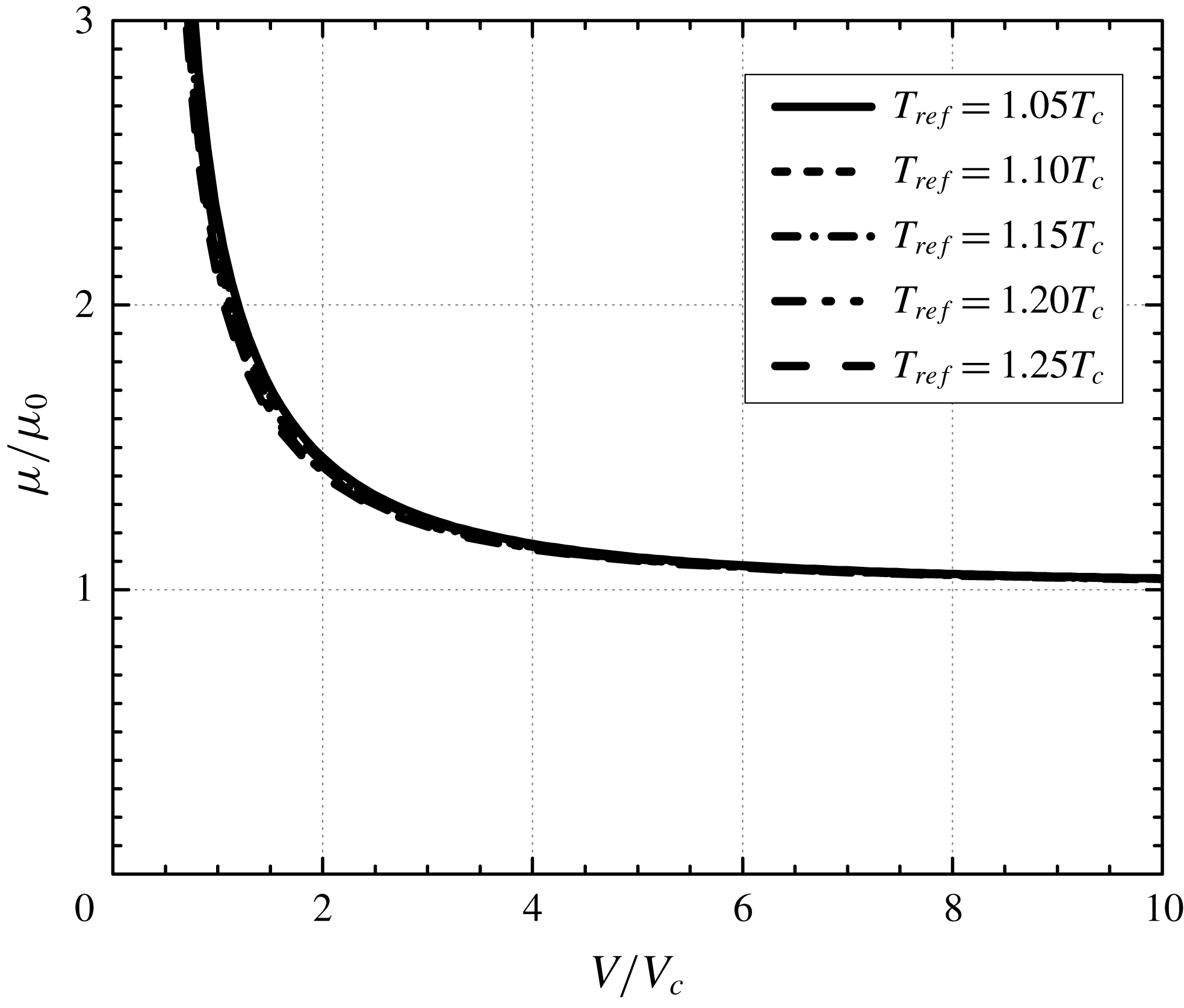
We next consider the lowest-order loss, i.e. the first term of (3.22), where $\overline{\unicode[STIX]{x1D707}}$ is evaluated at the lowest-order density. Following the conventional scaling used in the lubrication literature where the film thickness is scaled with the radial clearance, we have multiplied (3.22) by 1+ $\unicode[STIX]{x1D6FF}$ and have plotted this version of the scaled loss in figure 10 for various reference thermodynamic states. Inspection of figure 10 reveals that the reference temperature has an insignificant effect on the scaled loss. This is due to the fact that the shear viscosity roughly scales with the ideal gas shear viscosity, at least for the purposes of computing the temperature dependence. To illustrate this point, we have plotted the variation of the ratio of the shear viscosity to the ideal gas viscosity at the same temperatures in figure 11.

As indicated in the discussion of (3.25), the scaled loss for low-pressure gases will depend only on $\unicode[STIX]{x1D6FF}$ due to the fact that $\overline{\unicode[STIX]{x1D707}}=1$ in the ideal gas limit. Thus, each curve in figure 10 will approach the same low-pressure asymptote for fixed $\unicode[STIX]{x1D6FF}$ . We note that the loss has been scaled with the loss found when the load is zero, i.e. when $\unicode[STIX]{x1D6FF}\equiv 0$ . As a result, the scaled loss will always be larger than 1 as we approach the ideal gas limit. However, observation of figure 11 reveals that the viscosity will depend on the local density as the reference pressure is increased. Because the viscosity increases monotonically with increasing density, $\overline{\unicode[STIX]{x1D707}}<$ 1 over most of the fluid domain. An example of the viscosity variation with $\overline{x}$ is plotted for various thermodynamic states in figure 12. As result, the scaled loss will decrease and even become less than 1 as the reference pressure is increased. That is, for pressurized gases the scaled loss generated by non-concentric cylinders can be smaller than that corresponding to concentric cylinders.

Figure 12.

Variation of scaled viscosity with x/L for $T_{ref}=1.05T_{c}$ . The parameter $\unicode[STIX]{x1D6FF}=0.5$ .

Figure 13.

Attitude angle ( $\unicode[STIX]{x1D713}$ ) versus reference specific volume. The parameter $\unicode[STIX]{x1D6FF}=0.5$ and the speed number $\unicode[STIX]{x1D6EC}=50$ .

The effects of pressurization on the attitude angle are displayed in figure 13 for various reference temperatures at $\unicode[STIX]{x1D6EC}=50$ . Here we used the associated attitude angle $\unicode[STIX]{x1D713}\equiv \unicode[STIX]{x03C0}-\unicode[STIX]{x1D711}$ , i.e. the angle between the direction of the total force and the negative $x^{\prime }$ axis seen in figure 2. Inspection of figure 13 reveals that $\unicode[STIX]{x1D713}$ increases with pressurization for a fixed reference temperature. At $T_{ref}=1.05T_{c}$ pressurization results in 25.5 % increase of $\unicode[STIX]{x1D713}$ over the value of $\unicode[STIX]{x1D713}$ obtained at low pressure. The reason for this increase is due to the non-monotone variation of both $\overline{\unicode[STIX]{x1D705}}_{T}$ and $\overline{\unicode[STIX]{x1D705}}_{Te}$ leading to a smaller decrease in the size of the integrand in (3.17). At higher temperatures both $\overline{\unicode[STIX]{x1D705}}_{T}$ and $\overline{\unicode[STIX]{x1D707}}$ monotonically increase as the pressure is increases. Thus, the integrands in (3.19) will be smaller and the increase in $\unicode[STIX]{x1D713}$ will be smaller at higher temperatures.

Figure 14.

Scaled load versus $\unicode[STIX]{x1D6FF}$ at $V(0)=3V_{c}$ , $6V_{c}$ and $12V_{c}$ . The speed numbers were taken to be $\unicode[STIX]{x1D6EC}=20$ , 30, 40, 50, $\infty$ and the reference temperature $T_{ref}=1.15T_{c}$ . Symbols represent the exact scaled load computed from (2.13)–(2.15) in which the pressure variation was obtained from the Reynolds equation (2.8) and the equation of state. Lines denote the approximation of the scaled load (3.18). The lowest-order results, i.e. $\unicode[STIX]{x1D6EC}=\infty$ , are represented by ——. Results for $\unicode[STIX]{x1D6EC}=50$ are denoted by ▫ and – – – –, results for $\unicode[STIX]{x1D6EC}=40$ are denoted by ○ and – ⋅ – ⋅ –, results for $\unicode[STIX]{x1D6EC}=30$ are denoted by ♢ and — ⋅ ⋅ — and results for $\unicode[STIX]{x1D6EC}=20$ are denoted by ▵ and - - - -.

Figure 15.

Scaled loss versus $\unicode[STIX]{x1D6FF}$ at $V(0)=12V_{c}$ . The speed numbers are taken to be $\unicode[STIX]{x1D6EC}=20$ , 30, 40, 50, $\infty$ and the reference temperature $T_{ref}=1.15T_{c}$ . Symbols represent the exact scaled loss computed from (2.18). Lines denote the approximation of the scaled loss (3.22). The lowest-order results, i.e. $\unicode[STIX]{x1D6EC}=\infty$ , are represented by ——. Results for $\unicode[STIX]{x1D6EC}=50$ are denoted by ▫ and – – – –, results for $\unicode[STIX]{x1D6EC}=40$ are denoted by ○ and – – – –, results for $\unicode[STIX]{x1D6EC}=30$ are denoted by ♢ and — ⋅ ⋅ — and results for $\unicode[STIX]{x1D6EC}=20$ are denoted by ▵ and - - - -.

Figure 16.

Scaled loss versus $\unicode[STIX]{x1D6FF}$ at $V(0)=3V_{c}$ . The speed numbers are taken to be $\unicode[STIX]{x1D6EC}=20$ , 30, 40, 50, $\infty$ and the reference temperature $T_{ref}=1.15T_{c}$ . Symbols represent the exact scaled loss computed from (2.18). Lines denote the approximation of the scaled loss (3.22). The lowest-order results, i.e. $\unicode[STIX]{x1D6EC}=\infty$ , are represented by ——. Results for $\unicode[STIX]{x1D6EC}=50$ are denoted by ▫ and – – – –, results for $\unicode[STIX]{x1D6EC}=40$ are denoted by ○ and – ⋅ – ⋅ –, results for $\unicode[STIX]{x1D6EC}=30$ are denoted by ♢ and — ⋅ ⋅ — and results for $\unicode[STIX]{x1D6EC}=20$ are denoted by ▵ and - - - -.

A comparison of the approximate and the exact scaled load is plotted as a function of $\unicode[STIX]{x1D6FF}$ at $\unicode[STIX]{x1D6EC}=20$ , 30, 40, 50 and $\infty$ with various reference thermodynamic states in figure 14. The reference temperature is taken to be $T_{ref}=1.15T_{c}$ . The range of the speed numbers is selected to be within the general operating range described by previous investigators (Conboy Reference Conboy2013; Kim Reference Kim2016). From (1.4) the rotational speeds corresponding to $\unicode[STIX]{x1D6EC}=20$ at $V(0)=12V_{c}$ , $6V_{c}$ and $3V_{c}$ are found to be 8432 rpm, 14 221 rpm and 19 660 rpm, respectively. The solid lines denote the lowest-order theory and the broken lines represent the second-order approximation (3.18). At $V(0)=12V_{c}$ there is little variation of the load with $\unicode[STIX]{x1D6EC}$ and it is reasonable to suggest that the lowest-order approximation is sufficient to predict the scaled load for this range of $\unicode[STIX]{x1D6FF}$ . As the reference pressure increases, the scaled load increases as expected, and more importantly, the effect of $\unicode[STIX]{x1D6EC}$ on the scaled load is seen to become more significant. As a result, the second-order approximation is seen to be necessary to evaluate the load generated by pressurized gases. Even at $\unicode[STIX]{x1D6EC}=20$ it was found that the maximum discrepancy between the second-order approximation and the exact scaled load for the case of $V(0)=3V_{c}$ is 4.7 %.

In order to illustrate the effect of $\unicode[STIX]{x1D6EC}$ on the loss, we have plotted the approximate and exact scaled loss as a function of $\unicode[STIX]{x1D6FF}$ at $V(0)=12V_{c}$ and $3V_{c}$ in figure 15 and figure 16, respectively. The speed number $\unicode[STIX]{x1D6EC}=20$ , 30, 40, 50 and $\infty$ , and the reference temperature was taken to be $T_{ref}=1.15T_{c}$ . Examination of figure 15 indicates that the agreement between the approximate and exact scaled loss is excellent for each $\unicode[STIX]{x1D6EC}$ at $V(0)=12V_{c}$ . The maximum difference between the second-order approximation and the exact scaled loss is found to be 2.5 % at $\unicode[STIX]{x1D6EC}=20$ . The scaled loss is seen to decrease with the increase of $\unicode[STIX]{x1D6EC}$ and to increase monotonically as $\unicode[STIX]{x1D6FF}$ increases. At higher pressures, the rate of increase of the viscosity with increasing density is larger than in the low-pressure case so that the loss for the case $V(0)=3V_{c}$ has a local minimum located at $\unicode[STIX]{x1D6FF}\approx 0.2$ . At these higher pressures the difference between the exact and approximate solutions is larger than in the low-pressure examples. Nevertheless, the maximum difference between the exact solution and the $\unicode[STIX]{x1D6EC}=20$ approximation is less than 10 % for the chosen values of $\unicode[STIX]{x1D6FF}$ and $V(0)$ .

Figure 17.

Attitude angle versus $\unicode[STIX]{x1D6FF}$ at $V(0)=12V_{c}$ . The speed numbers are taken to be $\unicode[STIX]{x1D6EC}=20$ , 30, 40 and 50 and the reference temperature $T_{ref}=1.15T_{c}$ . The scaled attitude angle is defined as $\unicode[STIX]{x1D713}\equiv \unicode[STIX]{x03C0}-\unicode[STIX]{x1D711}$ , i.e. the angle between the direction of the load and the negative $x^{\prime }$ axis seen in figure 2. Symbols represent the exact scaled attitude angle computed from (2.13) and (2.14). Lines denote the approximation of the scaled attitude angle obtained from (3.19). Results for $\unicode[STIX]{x1D6EC}=50$ are denoted by ▫ and – – – –, results for $\unicode[STIX]{x1D6EC}=40$ are denoted by ○ and — ⋅ —, results for $\unicode[STIX]{x1D6EC}=30$ are denoted by ♢ and — ⋅ ⋅ — and results for $\unicode[STIX]{x1D6EC}=20$ are denoted by ▵ and - - - -.

Figure 18.

Attitude angle versus $\unicode[STIX]{x1D6FF}$ at $V(0)=3V_{c}$ . The speed numbers $\unicode[STIX]{x1D6EC}=20$ , 30, 40 and 50 and the reference temperature $T_{ref}=1.15T_{c}$ . The scaled attitude angle is defined as $\unicode[STIX]{x1D713}\equiv \unicode[STIX]{x03C0}-\unicode[STIX]{x1D711}$ , i.e. the angle between the direction of the load and the negative x $^{\prime }$ axis seen in figure 2. Symbols represent the exact scaled attitude angle computed from (2.13) and (2.14). Lines denote the approximation of the scaled attitude angle obtained from (3.19). Results for $\unicode[STIX]{x1D6EC}=50$ are denoted by ▫ and – – – –, results for $\unicode[STIX]{x1D6EC}=40$ are denoted by ○ and — ⋅ —, results for $\unicode[STIX]{x1D6EC}=30$ are denoted by ♢ and — ⋅ ⋅ — and results for $\unicode[STIX]{x1D6EC}=20$ are denoted by ▵ and - - - -.

The attitude angle $\unicode[STIX]{x1D713}$ is plotted as a function of $\unicode[STIX]{x1D6FF}$ at $T_{ref}=1.15T_{c}$ for $V(0)=12V_{c}$ and $3V_{c}$ in figure 17 and figure 18, respectively. The speed numbers were taken to be $\unicode[STIX]{x1D6EC}=20$ , 30, 40 and 50. Observation of figure 17 reveals that the agreement between the exact $\unicode[STIX]{x1D713}$ and the first-order approximate $\unicode[STIX]{x1D713}$ is seen to be very good for each $\unicode[STIX]{x1D6EC}$ at $V(0)=12V_{c}$ where the maximum discrepancy is found to be 4 % at $\unicode[STIX]{x1D6EC}=20$ . The scaled attitude angle decreases with the increase of $\unicode[STIX]{x1D6EC}$ and the decrease in $\unicode[STIX]{x1D6FF}$ . At $V(0)=3V_{c}$ , the first-order approximation of $\unicode[STIX]{x1D713}$ still has reasonable agreement with the exact $\unicode[STIX]{x1D713}$ when $\unicode[STIX]{x1D6EC}>$ 30. At $\unicode[STIX]{x1D6EC}=20$ , the maximum difference between the exact $\unicode[STIX]{x1D713}$ and approximate $\unicode[STIX]{x1D713}$ is found to be 10.6 %. We note that the non-zero attitude angle at $\unicode[STIX]{x1D6FF}=0$ is due to the fact that both $\overline{F}_{x^{\prime }}$ and $\overline{F}_{y^{\prime }}\longrightarrow 0$ at the same rate as $\unicode[STIX]{x1D6FF}\longrightarrow 0$ . The limiting value of $\unicode[STIX]{x1D713}$ can be found by taking $\unicode[STIX]{x1D6FF}\longrightarrow 0$ in (3.19), (3.12) and (3.17) yielding

(4.3) $$\begin{eqnarray}\unicode[STIX]{x1D713}\sim \frac{2\unicode[STIX]{x03C0}}{\unicode[STIX]{x1D6EC}}\quad \text{as }\unicode[STIX]{x1D6FF}\longrightarrow 0.\end{eqnarray}$$

Thus, $\unicode[STIX]{x1D713}$ at $\unicode[STIX]{x1D6FF}=0$ will be independent of the reference thermodynamic state. For $\unicode[STIX]{x1D6EC}=20$ , 30, 40 and 50, the values of $\unicode[STIX]{x1D713}$ at $\unicode[STIX]{x1D6FF}=0$ will be $18^{\circ }$ , $12^{\circ }$ , $9^{\circ }$ and $7.2^{\circ }$ , respectively. This non-zero limit of $\unicode[STIX]{x1D713}$ as $\unicode[STIX]{x1D6FF}$ vanishes is consistent with the finding of Gross et al. (Reference Gross, Matsch, Castelli, Eshel, Vohr and Wildmann1980) for ideal gases.

5 Summary

We have obtained approximate solutions for the load and loss of a two-dimensional, steady, compressible, laminar and single-phase flow between two non-concentric cylinders. Solutions are based on large $\unicode[STIX]{x1D6EC}$ expansions of the Reynolds equation (2.8) and are therefore valid at most pressures and temperatures in the single-phase regime and for all Navier–Stokes fluids; the primary exception is the neighbourhood of the thermodynamic critical point where (2.8) breaks down. In appendix A we have given the connection between the friction loss and the net heat flux so that the heat transfer is determined once the friction loss is.

In the limit of ideal gases, the work of Gross et al. (Reference Gross, Matsch, Castelli, Eshel, Vohr and Wildmann1980) suggests that the first corrections to the load and loss are $O(\unicode[STIX]{x1D6EC}^{-2})$ . The present study demonstrates that this ordering holds for general fluids, i.e. for both low- and high-pressure gases, as well.

The effects of pressurization and non-ideal gas behaviour have been illustrated primarily through the use of the lowest-order theory. Pressurization affects the load through the bulk modulus and it affects the loss through the density dependence of the shear viscosity. We found that the load scales with the reference bulk modulus $\unicode[STIX]{x1D705}_{T}|_{ref}$ so that the non-monotone variations of the bulk modulus can result in a non-monotone variation of the load. Isothermal pressurization is seen to result in significant increases in the load.

At moderate pressures, inspection of figures 7 and 10 suggests that $\unicode[STIX]{x1D6EC}|\overline{\boldsymbol{F}}|$ and ( $1+\unicode[STIX]{x1D6FF}$ ) $|\overline{P}|$ can be regarded as nearly constant for reference specific volumes of $V(0)>6V_{c}$ . At higher pressures, the dependence of the density on the bulk modulus and viscosity becomes more noticeable. As a result, the strong decrease in the loss and the increase in the load will require the use of pure numerical solutions or the approximations given here.

The second-order approximations for load and loss are compared to the exact values obtained based on the solutions to the Reynolds equation (2.8) for a range of $\unicode[STIX]{x1D6FF}$ in figures 14–16. These examples illustrate the dependence of the load and loss on the eccentricity parameter (2.2) and the speed number.

The lowest-order attitude angle ( $\unicode[STIX]{x1D713}\equiv \unicode[STIX]{x03C0}-\unicode[STIX]{x1D711}$ ) has been computed and is found to decrease with increasing $\unicode[STIX]{x1D6EC}$ . At constant $\unicode[STIX]{x1D6EC}$ and a fixed reference thermodynamic state, the attitude angle is seen to approximately increase linearly with $\unicode[STIX]{x1D6FF}$ , at least for the cases shown. The values of $\unicode[STIX]{x1D713}$ at $\unicode[STIX]{x1D6FF}=0$ are given by (4.3) and are seen to be independent of thermodynamic state.

In order to focus on the physical effects of pressurization and the structure of the approximation scheme, we have restricted attention to the relatively simple flow model of Chien et al. (Reference Chien, Cramer and Untaroiu2017a ); this model has been validated against numerical solutions to the full Navier–Stokes solutions in Chien et al. (Reference Chien, Cramer and Untaroiu2017a ,Reference Chien, Cramer and Untaroiu b ). Many of the observed features here are due to the density dependence of the material functions and will be present, to greater or lesser degrees, in more complex flows, including those involving turbulent and three-dimensional flows.