1. Introduction
The flow of an incompressible viscous fluid inside a porous medium has attracted the attention of researchers in various fields of science, such as geophysics, hydrology, civil engineering, chemical engineering, medical engineering, etc., owing to its fundamental importance (see Muskat Reference Muskat1937; Scheidegger Reference Scheidegger1960; Harr Reference Harr1962; Freeze & Cherry Reference Freeze and Cherry1979). Recently, it has received much more attention in environmental processes such as convective spreading of contaminants in a soil and the prediction of landslides arising from heavy rainfall (Nield & Bejan Reference Nield and Bejan2013). These environmental processes require accurate measurements of underground volumetric flow rate as well as an a priori understanding of its future behaviour. Studies related to viscous flow through a granular material that has a hollow space (which we refer to as a ‘macroscopic cavity’ or simply a ‘cavity’ hereafter) are very limited. However, there have been classical studies where viscous flow past a random spherical particles is considered. Some of the earlier studies pertaining to this can be found in Brinkman (Reference Brinkman1947), Tam (Reference Tam1969), Batchelor (Reference Batchelor1972), Childress (Reference Childress1972), Lundgren (Reference Lundgren1972), Howells (Reference Howells1974). The pioneering work of Brinkman (Reference Brinkman1947) calculated the viscous force exerted by a flowing fluid on a dense swarm of particles. The corresponding mean flow rate has been calculated by virtue of treating the swarm as a porous mass. He also added a viscous term (hereafter referred to as the Brinkman term) into Darcy's equation. Lundgren (Reference Lundgren1972) obtained a theoretical justification of the Brinkman term. Childress (Reference Childress1972) studied the viscous flow past a random array of identical non-overlapping spheres and calculated the force acting on any given sphere. The latter gave a qualitative support of the Brinkman term. Tam (Reference Tam1969) and Howells (Reference Howells1974) developed the fundamental solution of the Brinkman equation, and obtained the drag force on a particle in a random distribution of particles. In particular, Howells (Reference Howells1974) analysed the work of Childress (Reference Childress1972) and obtained a modified mean flow rate and resistance while considering higher-order approximations. The corresponding flow was termed as a shielded Stokes flow where the concept of a shielded Stokeslet was introduced (see Howells Reference Howells1974). These works mainly focussed on the resistive force on the sparse random array of small particles, but many situations are encountered in groundwater flow where a non-uniform distribution of void space is present, which motivated the present study.
The usual method to measure the groundwater flow is to (i) put through eight boreholes (observation wells) encircling a particular borehole (injection well); (ii) inject tracers, such as salt, dye and isotopes, into the central borehole; and (iii) observe the time and position that the injected tracer is detected. This method, however, is costly, time consuming because of the very slow ground water flow, difficult to estimate the effect of diffusion and absorption of the tracer, and may be harmful to the environment if the density of the tracer is increased to enhance the sensitivity. An accurate and direct method for flow-field measurement is the use of laser Doppler velocimetry (LDV). LDV is non-intrusive, local and instantaneous, but cannot be applied to opaque media including soils. LDV can be applied if we create a hollow space in the soil, where the velocity field is measured by scanning using an optical fibre probe for LDV in the clear fluid region. The measurement, however, is not free from the question whether the flow field is the same as that before the macroscopic cavity is created. Thus a theoretical correction or validation of the measured velocity field inside the cavity is of crucial importance to estimate the groundwater flow under natural conditions. To reduce the cost and time required for measuring underground water, difficulties associated with absorption and diffusion of the tracer, as well as environmentally unfavourable influences, the single boring method was developed, where a macroscopic cavity is created (as in the boring hole) and the velocity field is measured in it. The velocity field is measured either directly, i.e. by the use of LDV, or indirectly, i.e. by detecting the electric conductivity change at the electrodes encircling the test point. The single boring method, however, needs a correction, which is associated with creating the hollow space in an otherwise homogeneous porous media.
For this purpose, Sano (Reference Sano1983) calculated the flow of an incompressible fluid past a single circular cylindrical cavity in an otherwise uniform porous media. The flow field inside the cavity was assumed to be governed by the Stokes equation, while the flow filed outside the cavity was governed by the Darcy–Brinkman equation (see Brinkman Reference Brinkman1947; Tam Reference Tam1969; Batchelor Reference Batchelor1972; Childress Reference Childress1972; Lundgren Reference Lundgren1972; Howells Reference Howells1974), and the velocity and the stress components were assumed to be continuous at the boundary. The flow field was characterized by the ratio  $\zeta _0 \equiv R_0/ \sqrt {k}$, where
 $R_0$ is the radius of the cavity and
 $k$ is the permeability of the porous medium. As the parameter
 $\zeta _0$ increased, the effect of the presence of that cavity increased, so that the velocity at the centre
 $V_c$ tended to three times of the undisturbed flow
 $U_\infty$ and the volume flux into the cavity
 $Q$ tended to two times of
 $Q_\infty$, which was the volume flux passing through the same domain without that cavity. These results were experimentally confirmed by Momii et al. (Reference Momii, Jinno, Ueda, Motomura, Hirano and Honda1989), who measured the velocity field inside a cylindrical bore hole by LDV. In the real situation, the cross-section of the boundary is not necessarily a complete circle. Raja Sekhar & Sano (Reference Raja Sekhar and Sano2003) extended the calculation to a cavity that was slightly deformed from the circle and was oriented at an arbitrary angle with respect to the undisturbed flow. It was observed that an elongated cavity placing its long axis parallel to the undisturbed flow shows
 $U_0 \sim 3.5 U_\infty$, whereas it is
 $U_0 \sim 2.4 U_\infty$ when the long axis is placed across the flow.
The effect of the cavity is much enhanced for three-dimensional (3-D) cases. Raja Sekhar & Sano (Reference Raja Sekhar and Sano2000) calculated the flow of an incompressible fluid past a single spherical cavity in an otherwise uniform porous medium. As  $\zeta _0$ increased, the velocity at the centre
 $V_c$ was found to tend to six times of the undisturbed flow
 $U_\infty$ and the volume flux into the cavity
 $Q$ to three times of
 $Q_\infty$, which is the volume flux through the same domain without that cavity. These 3-D results were partially confirmed by Sano et al. (Reference Sano, Sano, Takagi and Yamada2013), who measured the velocity field inside a hemispherical cavity by LDV. If the far upstream velocity
 $U_\infty$ exceeds a certain critical value
 $U_c$, the grains at the cavity boundary can no longer sustain the structure, so that the grains of the upstream-side boundary are removed and are carried downstream (see Kaneko & Sano Reference Kaneko and Sano2005; Sano & Nagata Reference Sano and Nagata2006; Sano Reference Sano2011, Reference Sano2020). Repetition of these processes create a fluidized region toward the upstream direction, which will be discussed in § 6.
The flow field inside and outside of the quasi-two-dimensional (2-D) cavity, in which a few layers of grains are squeezed between two transparent parallel plates, was visualized by sodium fluorescein (see Kaneko & Sano Reference Kaneko and Sano2003, Reference Kaneko and Sano2005). The velocity field inside the quasi-2-D cavity satisfactorily agreed with that measured inside a cylindrical cavity (see Momii et al. Reference Momii, Jinno, Ueda, Motomura, Hirano and Honda1989) as well as that from the 2-D calculation (see Sano Reference Sano1983), which supported the visualization experiment both in and outside of the quasi-2-D cavity. Interaction of two cavities  $C_1$ and
 $C_2$ of the same radius
 $R_0$ with arbitrary configuration was examined systematically by the above-mentioned visualization using the quasi-2-D system. The dependence of the volume flux into the downstream-side cavity
 $Q_2$ on the centre-to-centre distance of the cavities
 $l$ and the orientation
 $\alpha$ with respect to the undisturbed flow were elucidated (see Kaneko & Sano Reference Kaneko and Sano2003). It was found that
 $Q_2$ increases by approximately 20 % in some configuration (around
 $l^* (\equiv l/R_0) \sim 2$ and
 $\alpha \approx 15^{\circ }$), while it decreases by approximately 20 % in another configuration (around
 $l^* \sim 2$ and
 $\alpha \approx 90^{\circ }$). These results were reproduced by numerical simulation (Sano & Nagata Reference Sano and Nagata2006). The interaction of two cavities, in which the asymptotic effect of the other cavity is taken into account, was analysed (see Sano Reference Sano2020), which also reproduced the experimental findings. As a result of interaction, the critical value
 $U_c$, where the collapse of cavities results, may be lowered, and the spread of the fluidized region may be enlarged, so that the network formation of the water channel and the onset of a landslide arising from heavy rainfalls may be predicted (see Kaneko & Sano Reference Kaneko and Sano2005; Sano & Nagata Reference Sano and Nagata2006; Sano Reference Sano2011, Reference Sano2020), which will be discussed in § 6. We found that the concentration of the flow and the stresses are more pronounced in the 3-D configuration, which is often the case in real situations. The first-order calculation of the interaction of two equally sized spherical cavities has been examined (see Sano Reference Sano2008), in which the far-field results of the single 3-D cavity are superposed in the porous region, but further studies, either experimental or numerical, have been limited. Much of the available theoretical results come from the research groups of the present authors, as reviewed in this section. Motivated by these circumstances, we extend here to the interaction of 3-D cavities. Similar to the 2-D case, we consider an unbounded granular material (porous medium) which hosts two spherical cavities. We assume that the flow inside the cavities is governed by the Stokes equation, while it is governed by the Darcy–Brinkman equation inside the granular bed. We reproduced a 3-D singularity termed here as ‘Darcylet’, which is a fundamental solution in the granular material that was originally described by Howells (Reference Howells1974), and acts like a point force along the flow. We apply it to obtain the 3-D flow in a porous media with macroscopic cavities by the use of Stokes and Darcy–Brinkman equations. Understanding the interaction of the 3-D cavities provides insight to predict more realistic applications like the network formation of the water channel and the onset of a landslide arising from heavy rainfalls. The mechanical balance of the force, which includes gravity, is initially assumed to be maintained by the friction between contacting grains before the collapse irrespective of the presence of a fluid. Note that the granular material is blocked or in a jamming state for highly concentrated and/or lower sheared conditions (see Duran Reference Duran1997; Liu & Nagel Reference Liu and Nagel1998; Majmudar & Behringer Reference Majmudar and Behringer2005; Behringer Reference Behringer2015; Morris Reference Morris2020). Because of the finite size of grains (‘excluded volume effect’), the force balance in granular materials under gravity and other applied stress is achieved by local arching, or the formation of stress chains between grains, which holds even in the presence of hollow spaces larger than the prevailing interstices between grains. Granular mechanics revealed that even if destruction of stress chains may occur in the jamming state, it is rather localized so that the static frictional forces balance, and hence the global structure, is maintained. Such a jamming state may be encountered in newly piled-up sand hills or inhomogeneous strata. We focus our attention on the fluid mechanical aspects immediately before the collapse of the existing structure. However, once destruction occurs, either by vibration (as in earthquakes) or by flow concentration (as in heavy rainfalls), global granular flows may be caused until some new quasi-equilibrium state is reached. For such granular flows, quite a number of investigations have been conducted without a fluid (see MiDi Reference MiDi2004; Aranson & Tsimring Reference Aranson and Tsimring2006) and/or with a fluid (see Campbell Reference Campbell1990; Forterre & Pouliquen Reference Forterre and Pouliquen2008; Gray Reference Gray2018; Morris Reference Morris2020). The latter deals with shear thickening of concentrated suspensions, which leads to solidification or jamming in certain circumstances. Our study will add new insights to the still remaining gap between the solid and fluid states. The present analysis also finds a place in several biological processes owing to its resemblance with blood flow through a collection of cells in human tissues and organs. Further discussion will be given in § 6.
2. Method of calculation
2.1. Fundamental solution of the flow through a single cavity in a granular material
2.1.1. Governing equations
We consider a single spherical macroscopic hollow space of radius  $R_0$ (hereafter referred to as a ‘cavity’) in an otherwise homogeneous granular material that is exposed to a uniform flow
 $U_\infty$ at infinity, while assuming the domain is sufficiently large. We assume that the flow inside the cavity is governed by the Stokes equation,
 \begin{equation} \mu \Delta {\boldsymbol{v}^*}=\boldsymbol{\nabla} p^*, \end{equation}
where  ${\boldsymbol {v}^*}$ and
 $p^*$ are the velocity and pressure of the fluid, which is assumed incompressible,
 \begin{equation} \boldsymbol{\nabla} \boldsymbol{\cdot} \boldsymbol{v}^*=0, \end{equation}
and  $\mu$ is the viscosity. The flow outside the cavity is assumed to be governed by the Darcy–Brinkman equation,
 \begin{equation} \frac{\mu}{k} {\boldsymbol{v}^*} ={-} \boldsymbol{\nabla} p^* +\mu_{e} \Delta {\boldsymbol{v}^*}, \end{equation}
where  $k$ is the permeability of the otherwise homogeneous granular material and
 $\mu _{e}$ is the effective viscosity. Existing literature shows that different models have been used to appraise the effective viscosity
 $\mu _{e}$ inside porous media. These investigations show a dependency of
 $\mu _{e}$ on
 $\mu$, which however differs whether
 $\mu _{e}>\mu$ or
 $\mu _{e}<\mu$ or equals to
 $\mu$ depending upon the distribution of pores inside the medium (see Givler & Altobelli Reference Givler and Altobelli1994; Martys, Bentz & Garboczi Reference Martys, Bentz and Garboczi1994; Ochoa-Tapia & Whitaker Reference Ochoa-Tapia and Whitaker1995; Nield & Bejan Reference Nield and Bejan2013). In the present study, to circumvent the controversy and to focus on the initiation of cavity collapse in a granular material, we make the assumption
 $\mu _{e}=\mu$. This set of equations (2.1a–c) is to be solved under the conditions that the velocity and stress are continuous at the cavity boundary in addition to the boundary condition at infinity.
One may attempt to develop a series solution or a numerical solution for the boundary value problem defined above. However, in this manuscript, we wish to consider the singularity method which is quite effective to capture the solution of the Darcy–Brinkman equation in terms of Green's function. Correspondingly, we shall first consider the Darcy–Brinkman equation with a force singularity,
 \begin{equation} \frac{\mu}{k} {\boldsymbol{v}^*} ={-} \boldsymbol{\nabla} p^* +\mu \Delta {\boldsymbol{v}^*} +{\boldsymbol F}^*\delta^* (\boldsymbol{R}^*), \end{equation}
where  ${\boldsymbol R^*}={\boldsymbol {x^*}} - {\boldsymbol {x^*}}'$ and
 ${\boldsymbol {x^*}}'$ is the position of the singularity. We use the following non-dimensional variables:
 \begin{equation} \left.\begin{gathered}
\displaystyle {\boldsymbol x}=\dfrac{{\boldsymbol
x}^*}{R_0},\quad {\boldsymbol v}=\dfrac{{\boldsymbol
v}^*}{U_\infty}, \quad p=\dfrac{p^*}{\mu U_\infty /R_0},
\quad {\boldsymbol F}=\dfrac{{\boldsymbol F}^*}{ \mu R_0
U_\infty}, \quad
\boldsymbol{R}=\dfrac{\boldsymbol{R}^{*}}{R_{0}},\\
\displaystyle \delta({\boldsymbol R})= R_0^3 {\boldsymbol
\delta}^*(\boldsymbol{R}^*), \quad
\zeta_{0}=\dfrac{R_{0}}{\sqrt{k}}.
\end{gathered}\right\} \end{equation}
By the use of non-dimensional variables, (2.1a)–(2.1c) become
 $$\begin{gather} \Delta {\boldsymbol{v}}=\boldsymbol{\nabla} p, \end{gather}$$
 $$\begin{gather}\boldsymbol{\nabla} \boldsymbol{\cdot} \boldsymbol{v}=0, \end{gather}$$
 $$\begin{gather}(\varDelta - \zeta_0^2 )\boldsymbol{v} = \boldsymbol{\nabla} p. \end{gather}$$
The corresponding Darcy–Brinkman equation with a forced singularity term in non-dimensional form becomes
 \begin{equation} (\varDelta - \zeta_0^2) {\boldsymbol{v}} =\boldsymbol{\nabla} p - {\boldsymbol F}\delta(\boldsymbol{R}). \end{equation}
For further developments, we need the solution of the Darcy–Brinkman equation with a 3-D forced singularity given in (2.6), i.e. Green's function of the Darcy–Brinkman equation. The same is discussed in § 2.1.2
2.1.2. Darcylet
Hereafter, we choose the position of the singularity at  $\boldsymbol {x'}=0$ and denote
 $\boldsymbol {R}^{*}$,
 $\boldsymbol {R}$ and
 $R~(=|\boldsymbol {R}|)$ as
 $\boldsymbol {r}^{*}$,
 $\boldsymbol {r}$ and
 $r~(=|\boldsymbol {r}|)$, respectively. Taking the divergence of (2.6) that satisfies (2.4) is given by (see Appendix A for details)
 $$\begin{gather} p=\frac{{\boldsymbol F}\boldsymbol{\cdot} {\boldsymbol r}}{4{\rm \pi} r^3}. \end{gather}$$
 $$\begin{gather}{\boldsymbol v}=\frac{1}{4{\rm \pi} \zeta_0^2} \left[\left(f(r)\, \textrm{e}^{-\zeta_0 r}-\frac{1}{r^3}\right){\boldsymbol F} - \frac{({\boldsymbol F}\boldsymbol{\cdot}{\boldsymbol r}) {\boldsymbol r} }{r^2}\left(g(r)\, \textrm{e}^{-\zeta_0 r}- \frac{3}{r^3}\right)\right], \end{gather}$$
where
 \begin{equation} f(r)=\frac{\zeta_0^2}{r}+\frac{\zeta_0}{r^2}+\frac{1}{r^3}, \quad g(r)=\frac{\zeta_0^2}{r}+\frac{3\zeta_0}{r^2}+\frac{3}{r^3}.\end{equation}
The velocity field at  $\boldsymbol {x}$ arising from the Darcylet at
 $\boldsymbol {x'}$ is generally expressed as
 $v_i=T^D_{ij}(\boldsymbol {x}-\boldsymbol{x'}) {F}_j(\boldsymbol {x'})$, where
 \begin{align} T^D_{ij}({\boldsymbol x})=\frac{1}{4{\rm \pi} \zeta_0^2}[ h_{ij}({\boldsymbol x})+H_{ij}({\boldsymbol x})], \quad h_{ij}({\boldsymbol x})=\left(f(r)\delta_{ij} - \frac{x_i x_j }{r^2}g(r)\right) \textrm{e}^{-\zeta_0 r}, \quad H_{ij}({\boldsymbol x})={-}\frac{\delta_{ij}}{r^3}+ \frac{3x_i x_j }{r^5},\end{align}
which is the same as that derived by Tam (Reference Tam1969) and then Howells (Reference Howells1974), except the constant of proportion  $8{\rm \pi}$.
This tensor may be termed as the ‘Darcy’ tensor corresponding to the Oseen tensor in the Stokes flow. Note that  $\Delta h_{ij}({\boldsymbol x})=\zeta _0^2 h_{ij}({\boldsymbol x})$ and
 $\Delta H_{ij}({\boldsymbol x}) = 0$ at
 ${\boldsymbol x} \ne {\boldsymbol 0}$. The part of (2.10),
 $v_i= {F}_j /(4{\rm \pi} \zeta _0^2) H_{ij}$ and
 $p$ given by (2.7) also constitute the Darcy flow
 ${\boldsymbol v}= - \boldsymbol {\nabla } p/\zeta _0^2$, but we shall denote here the set of expressions (2.8) and (2.7) by a ‘Darcylet’. The asymptotic behaviour of
 $T^D_{ij}$ is
 \begin{equation} T^D_{ij}(\boldsymbol x) =\frac{1}{8{\rm \pi}}\left(\frac{\delta_{ij}}{r} + \frac{x_i x_j}{r^3} -\frac{4}{3}\zeta_0 \delta_{ij} +O(\zeta_0^2) \right) \quad \textrm{for}\ \zeta_0 \ll 1, \end{equation}
and
 \begin{equation} T^D_{ij}(\boldsymbol x) =\frac{1}{4{\rm \pi} \zeta_0^2}\left( - \frac{\delta_{ij}}{r^3} +\frac{3x_i x_j}{r^5}\right) \quad \textrm{for}\ \zeta_0 \gg 1.\end{equation}
In the former, the cavity size is small and indistinguishable from the interstice of the grains, so that the leading term is the same as the Stokeslet in a homogeneous material. However, the latter is of the form of a potential dipole, because of highly packed grains outside the cavity, which shield the viscous effect from the boundary.
The stress components  $\tau _{ij}$ are given by
 \begin{align} 4{\rm \pi} \zeta_0^2\ \tau_{ij} &=\frac{({\boldsymbol F}\boldsymbol{\cdot}{\boldsymbol r})}{r}\left[-\frac{\zeta_0^2}{r^2}+\frac{6}{r^4} -2\left(\frac{\zeta_0^2}{r^2}+\frac{3\zeta_0}{r^3}+\frac{3}{r^4}\right) \textrm{e}^{-\zeta_0 r}\right] \delta_{ij}\nonumber\\ &\quad +\frac{{F}_i x_j+{F}_j x_i}{r}\left[\frac{6}{r^4} -\left(\frac{\zeta_0^3}{r}+\frac{3\zeta_0^2}{r^2} +\frac{6\zeta_0}{r^3}+\frac{6}{r^4}\right) \textrm{e}^{-\zeta_0 r}\right]\nonumber\\ &\quad +\frac{2({\boldsymbol F}\boldsymbol{\cdot}{\boldsymbol r}) x_i x_j }{r^3} \left[- \frac{15}{r^4} +\left(\frac{\zeta_0^3}{r}+\frac{6\zeta_0^2}{r^2}+\frac{15\zeta_0}{r^3} +\frac{15}{r^4}\right) \textrm{e}^{-\zeta_0 r}\right]. \end{align}
Equation (2.12) is the same as that given by Kohr & Raja Sekhar (Reference Kohr and Raja Sekhar2007). The asymptotic forms are
 \begin{equation} \tau_{ij} ={-} \frac{3({\boldsymbol F}\boldsymbol{\cdot}{\boldsymbol r}) x_i x_j}{4{\rm \pi} r^5} +O(\zeta_0^2) \quad \textrm{for} \ \zeta_0 \ll 1, \end{equation}
and
 \begin{equation} \tau_{ij} ={-} \frac{({\boldsymbol F}\boldsymbol{\cdot}{\boldsymbol r}) }{4{\rm \pi} r^3} \delta_{ij} \quad \textrm{for} \ \zeta_0 \gg 1. \end{equation}
The former is the same as that owing to a Stokeslet of magnitude  $- F^*/8{\rm \pi} \mu$. However, the latter shows that only the pressure contributes to the stress.
2.1.3. Darcylet in the  $x$ direction

As a special case, let the force be in the  $x$ direction
 ${\boldsymbol F}=(F,0,0)$ at the origin. Then the solutions (2.7) and (2.8) are expressed by
 $$\begin{gather} p=\frac{F}{4{\rm \pi}} \frac{x}{r^3}, \quad v_x=\frac{F}{4{\rm \pi}\zeta_0^2}\left[ \left(f(r) - \frac{x^2}{r^2} g(r)\right) \textrm{e}^{-\zeta_0 r} -\frac{1}{r^3}+\frac{3x^2}{r^5} \right], \end{gather}$$
 $$\begin{gather}v_y=\frac{F}{4{\rm \pi}\zeta_0^2}\left( - \frac{xy}{r^2} g(r) \, \textrm{e}^{-\zeta_0 r} + \frac{3xy}{r^5} \right), \quad v_z=\frac{F}{4{\rm \pi}\zeta_0^2}\left( - \frac{xz}{r^2} g(r) \, \textrm{e}^{-\zeta_0 r} + \frac{3xz}{r^5} \right). \end{gather}$$
In the spherical polar coordinate system  $(r, \theta, \varphi )$ with its polar axis in the
 $x$ direction, we have
 $v_\varphi =0$ and
 $$\begin{gather} p =\frac{F}{4{\rm \pi}} \frac{\cos\theta}{r^2}, \quad v_r=\frac{F}{4{\rm \pi}\zeta_0^2}\left[{-}2 \left( \frac{\zeta_0}{r^2}+\frac{1}{r^3} \right) \textrm{e}^{-\zeta_0 r} +\frac{2}{r^3} \right]\cos\theta, \end{gather}$$
 $$\begin{gather}v_\theta= \frac{F}{4{\rm \pi}\zeta_0^2} \left({-}f(r) \, \textrm{e}^{-\zeta_0 r} +\frac{1}{r^3}\right)\sin\theta. \end{gather}$$
The stream function is given by
 \begin{equation} \varPsi=\frac{F}{4{\rm \pi}\zeta_0^2}\frac{\sin^2\theta}{r} [1-(1+\zeta_0 r) \, \textrm{e}^{-\zeta_0 r}]. \end{equation}
Asymptotic behaviour of  $\varPsi$ is
 \begin{equation} \varPsi \sim \frac{F}{8{\rm \pi}} r \sin^2\theta+O(\zeta_0 r^2) \quad \textrm{for} \ \zeta_0 r \ll 1 \end{equation}
and
 \begin{equation} \varPsi \sim \frac{F}{4{\rm \pi}\zeta_0^2} \frac{\sin^2\theta}{r} \quad \textrm{for} \ \zeta_0 r \gg 1. \end{equation}
The former is the same as a Stokeslet of strength  ${ F}(=F^*/(8{\rm \pi} \mu )$, whereas the latter is the potential dipole of strength
 ${F}/(4{\rm \pi} \zeta _0^2)$.
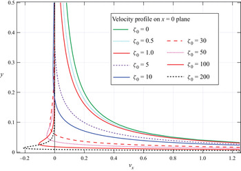
From (2.14b), we have the velocity profile on the  $x=0$ plane,
 \begin{equation} {v_x} = \frac{F}{{4{\rm \pi} \zeta _0^2}}\frac{{{\zeta _0}y(1 + {\zeta _0}y)\,{\textrm{e}^{ - {\zeta _0}y}} - (1 - {\textrm{e}^{ - {\zeta _0}y}})}}{{{y^3}}}, \end{equation}
which is shown in figure 1. Here  $y$ is the distance from the
 $x$-axis. As
 $\zeta _0$ tends to 0, it approaches to that owing to a Stokeslet (Stokeslet in non-dimensional form is
 $v_x = ({F}/{8{\rm \pi} }) ( {1}/{r}+{x^2}/{r^3}) \sim F/(8{\rm \pi} y),$ on the
 $x=0$ plane, where
 $r=y(>0)$ in the meridian plane),
 \begin{equation} {v_x}\sim \frac{F}{8{\rm \pi} y} \left(1-\frac{4}{3}\zeta_0 y +\cdots \right) \quad \textrm{or}\quad {v_x}^*\sim \frac{{F^*}}{{8{\rm \pi} \mu}}\left(\frac{1}{ y^*}-\frac{4}{3\sqrt{k}}\zeta_0 +\cdots \right),\end{equation}
while it approaches the potential dipole as  $\zeta _0$ tends to infinity (with
 $y \ne 0)$,
 \begin{equation} {v_x}\sim{-} \frac{F}{{4{\rm \pi} \zeta _0^2{y^3}}} \quad \textrm{or}\quad {v_x}^*\sim{-} \frac{{kF^*}}{{4{\rm \pi} \mu {{y^*}^3}}}. \end{equation}
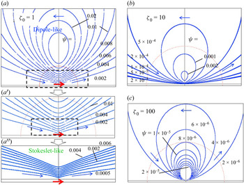
We also show the streamlines owing to a Darcylet in figure 2. These figures also show the Stokeslet-like features near the singularity (figure 2a  $''$), while they show dipole-like features as a far-field (figures 2b and 2c).
Velocity profile of Darcylet on the  $x=0$ plane.

Streamlines owing to a Darcylet at the centre with (a)  $\zeta _0=1$, (b)
 $\zeta _0=10$, (c)
 $\zeta _0=100$, where (a
 $'$) and (a
 $''$) are the close-up views of (a).

2.1.4. Strength of the Darcylet and the hydrodynamic force
We shall calculate the hydrodynamic force  $\tilde {F}_i$ given by the Darcylet of strength
 ${\boldsymbol F}$. To do this, we calculate the stress over the cavity boundary
 $S_0$ (spherical surface of normalized radius 1),
 \begin{equation} \tilde{F}_i= \int_{S_0} \tau_{ij} n_j \, \textrm{d} S ={-}\frac{1}{3} F_i [1+2(1+\zeta_0)\, \textrm{e}^{-\zeta_0}]. \end{equation}
If there is no discernible cavity (i.e.  $\zeta _0 \ll 1$),
 $\tilde {F}_i=-F_i$, as is expected from the action–reaction law. However, for
 $\zeta _0 \gg 1$,
 $\tilde {F}_i= - (1/3) F_i$, which reflects the strong shielding effect.
In terms of the force  $\tilde {\boldsymbol F}$, expressions in the subsections of § 2 are given by replacing
 $F_i$ by
 \begin{equation} F_i={-}\frac{3\tilde{F}_i}{1+2(1+\zeta_0)\, \textrm{e}^{-\zeta_0}}. \end{equation}
It is well known that the governing equations for the oscillatory Stokes flow are similar to the Darcy–Brinkman equations except that the permeability parameter and the frequency parameter have their own physical meanings. In this context, we recall that the expression for the drag force acting on a spherical surface  $r$ having the centre at the oscillating force agrees well with the expressions for the drag given above (see Kohr & Pop Reference Kohr and Pop2004).
3. Flow through a granular medium with a single spherical cavity
In this section, we shall consider the flow through a granular medium with a single spherical cavity in terms of a Darcylet, which was developed in the previous section. This approach should serve as a compact tool to handle more complicated situations as dealt in the next section.
(i) Fundamental flows outside the cavity
The flow outside the cavity  $(r \ge 1)$ is governed by the Darcy–Brinkman equation, which will be given by the uniform Darcy flow
 $U_i$ in the
 $x_i$ direction,
 \begin{equation} p={-}\zeta_0^2 U_k x_k, \quad v_i = U_{i}, \quad \tau_{ij}= \zeta_0^2 U_k x_k\delta_{ij}, \end{equation}
the Darcylet of magnitude  $F_i$ (particular solution of (2.4) and (2.6)),
 \begin{equation} p=\frac{F_k}{4{\rm \pi}} H_k, \quad v_i= \frac{F_k}{4{\rm \pi} \zeta_0^2}(h_{ik}+H_{ik}), \end{equation}
where
 \begin{equation} h_{ij}=\left(f(r)\delta_{ij}-\frac{x_i x_j}{r^2}g(r)\right) \textrm{e}^{-\zeta_0 r}, \quad H_i = \frac{x_i}{r^3},\quad H_{ij}={-}\frac{\delta_{ij}}{r^3}+ \frac{3x_i x_j }{r^5}, \end{equation}
and
 \begin{align} \tau_{ij}= \frac{F_k}{4{\rm \pi} \zeta_0^2}\left\{ [- x_k G_1(r)\delta_{ij}-(x_i \delta_{jk}+x_j \delta_{ik})G_2(r) + x_i x_j x_kG_3(r)]\, \textrm{e}^{-\zeta_0 r} - \zeta_0^2 H_k\delta_{ij}+6H_{ijk} \right\}, \end{align}
where
 $$\begin{gather} G_1(r)=\frac{2}{r^2}\left( \frac{\zeta_0^2}{r}+\frac{3\zeta_0}{r^2}+\frac{3}{r^3}\right),\quad G_2(r)=\frac{1}{r^2} \left(\zeta_0^3+ \frac{3\zeta_0^2}{r}+\frac{6\zeta_0}{r^2}+\frac{6}{r^3}\right), \end{gather}$$
 $$\begin{gather}G_3(r)=\frac{2}{r^4} \left(\zeta_0^3+ \frac{6\zeta_0^2}{r}+\frac{15\zeta_0}{r^2}+\frac{15}{r^3}\right), \quad H_{ijk}=\frac{x_i \delta_{jk}+x_j \delta_{ki}+x_k \delta_{ij} }{r^5}-\frac{5 x_i x_j x_k}{r^7}, \end{gather}$$
and the Darcy flow of magnitude  $C_i$ (general solution of the homogeneous parts of (2.4) and (2.6)),
 \begin{equation} p=\zeta_0^2 C_k H_k, \quad v_i = C_k H_{ik}, \quad \tau_{ij}= C_k(-\zeta_0^2 H_k\delta_{ij}+6 H_{ijk}).\end{equation}
(ii) Fundamental flows inside the cavity
The flow inside the cavity  $(r \le 1)$ is governed by the Stokes equation, which will be described by the Stokeson of magnitude
 $A_i$ (see Chwang & Wu Reference Chwang and Wu1974, Reference Chwang and Wu1975),
 \begin{equation} p=10A_k x_k, \quad v_i=A_k(2r^2 \delta_{ik}-x_i x_k), \quad \tau_{ij}= 3A_k (x_i\delta_{jk}+x_j\delta_{ik}- 4 x_k\delta_{ij}), \end{equation}
and the uniform Stokes flow of magnitude  $B_i$,
 \begin{equation} p=p_0 ({=}0), \quad v_i =B_i, \quad \tau_{ij}={-}p_0 \delta_{ij} ({=}0).\end{equation}
(iii) By superposing these fundamental flows inside and outside of the cavity, and imposing the condition that the velocity components and stress components are continuous at the boundary  $r=1$, we obtain the flow field. As an example, if we consider the uniform flow at infinity in the
 $x_1$ direction, i.e.
 $U_i=\delta _{i1}$, we have, after tedious but straightforward calculation,
 $$\begin{gather} A_1={-} \frac{3\zeta_0^2(1+\zeta_0)}{\varDelta_0},\quad B_1=\frac{3(2\zeta_0^3+7\zeta_0^2+15\zeta_0+15)}{\varDelta_0}, \quad \frac{F_1}{4{\rm \pi} \zeta_0^2} =\frac{15 \, \textrm{e}^{\zeta_0}}{\varDelta_0} ({\equiv} D_1), \end{gather}$$
 $$\begin{gather}E_1 =\frac{\varDelta_1}{\varDelta_0} ({\equiv} C_1+D_1), \quad \varDelta_0=\zeta_0^3+6\zeta_0^2+45\zeta_0+45, \quad \varDelta_1=\zeta_0^3+6\zeta_0^2+15\zeta_0+15, \end{gather}$$
other coefficients being zero, which agree with our previous results (see Raja Sekhar & Sano Reference Raja Sekhar and Sano2000).
In terms of the spherical coordinate system, the above expressions are given as follows.
Outside of the cavity ( $r \ge 1$):
 $$\begin{gather} p= {\zeta_0}^2\left( - r+\frac{E_1}{r^2}\right)\cos\theta , \quad v_r=\left[1 - 2D_1\left( \frac{\zeta_0}{r^2}+\frac{1}{r^3} \right) \textrm{e}^{-\zeta_0 r} +\frac{2E_1}{r^3} \right] \cos\theta, \end{gather}$$
 $$\begin{gather}v_\theta=\left({-}1 - D_1 f(r) \, \textrm{e}^{-\zeta_0 r} +\frac{E_1}{r^3} \right) \sin\theta, \end{gather}$$
 $$\begin{gather}\tau_{rr}=\left[\zeta_0^2 r + \frac{4D_1}{r} g(r) \, \textrm{e}^{-\zeta_0 r} - E_1 \left( \frac{\zeta_0^2 }{r^2}+\frac{12}{r^4} \right)\right]\cos\theta, \end{gather}$$
 $$\begin{gather}\tau_{\theta r}= \left[D_1\left(\frac{\zeta_0^3}{r}+\frac{3\zeta_0^2}{r^2} +\frac{6\zeta_0}{r^3}+\frac{6}{r^4}\right) \textrm{e}^{-\zeta_0 r} -\frac{6E_1 }{r^4}\right] \sin\theta, \end{gather}$$
 $$\begin{gather}\varPsi=\sin^2\theta \left(\frac{1}{2}r^2-\frac{D_1}{r}(1+\zeta_0 r) \, \textrm{e}^{-\zeta_0 r} +\frac{E_1}{r}\right). \end{gather}$$
Inside the cavity ( $r \le 1$):
 $$\begin{gather} p=10A_1 r \cos\theta, \quad v_r=(A_1 r^2+B_1) \cos\theta,\quad v_\theta ={-}(2A_1 r^2+B_1) \sin\theta, \end{gather}$$
 $$\begin{gather}\tau_{rr}={-}6A_1r\cos\theta,\quad \tau_{\theta r}={-} 3A_1r\sin\theta, \end{gather}$$
 $$\begin{gather}\varPsi=\tfrac{1}{2} \sin^2 \theta (A_1r^4+B_1r^2). \end{gather}$$
If we rewrite (3.9),
 \begin{align} \varPsi=\sin^2\theta\left\{\frac{1}{2}r^2 + \frac{15 \, \textrm{e}^{\zeta_0}}{\varDelta_0 }\frac{1}{r}\times [1-(1+\zeta_0 r) \, \textrm{e}^{-\zeta_0 r}] +\frac{\zeta_0^3+6\zeta_0^2+15\zeta_0+15 -15 \, \textrm{e}^{\zeta_0}}{\varDelta_0}\times\frac{1}{r} \right\}, \end{align}
it is easily understood that the first and third terms in the right-hand side of (3.13) describe the uniform flow and the potential dipole, respectively, while the second term is the contribution of the Darcylet.
In particular, for  $\zeta _0 \gg 1$,
 \begin{equation} \left.\begin{gathered}
\displaystyle A_1
={-}3\left(1-\dfrac{5}{\zeta_0}+O(\zeta_0^{{-}2})
\right),\quad B_1 = 6
\left(1-\dfrac{5}{2\zeta_0}+O(\zeta_0^{{-}2}) \right),\\
\displaystyle D_1 = \dfrac{15\,
\textrm{e}^{\zeta_0}}{\zeta_0^3}\left(1-\dfrac{6}{\zeta_0}+O(\zeta_0^{{-}2})
\right), \quad E_1 = 1+O(\zeta_0^{{-}2}),
\end{gathered}\right\} \end{equation}
so that the approximate expressions of stream function are
 \begin{equation} \varPsi_1 = \sin^2\theta \left[\frac{1}{2}r^2 -\frac{15}{\zeta_0^3 }\left(1-\frac{6}{\zeta_0}\right) \frac{(1+\zeta_0 r) \, \textrm{e}^{-\zeta_0 (r-1)}}{r}+\frac{1}{r} \right], \quad r\ge 1, \end{equation}
and
 \begin{equation} \varPsi_1 = 3 \sin^2\theta\ r^2 \left( 1-\frac{1}{2}r^2 - \frac{5}{2\zeta_0}(1-r^2)\right), \quad r\le 1. \end{equation}
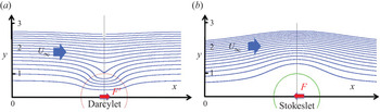
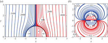
We show a typical flow field in figure 3(a). For comparison, the Stokes flow past a solid sphere at rest is shown in figure 3(b). In the latter, fluid motion is decelerated because of the presence of the solid body (or owing to the Stokeslet directed adversely to the main flow), which blocks the stream and hence, the separation distances between the streamlines become wider near the axis. However, in the former, fluid motion is accelerated (because of the Darcylet directed along the main flow), so that the separation distances between the streamlines become narrower near the axis.
(a) A spherical cavity in granular material exposed to a uniform flow at infinity. (b) Stokes flow past a solid sphere.

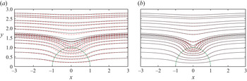
We also show streamlines for the typical cases  $\zeta _0 = 10$ and
 $40$ in figure 4. For comparison, exact calculations of the streamlines are shown as black lines. For the larger
 $\zeta _0$ cases, the flow field looks well described by the first approximation
 $\varPsi _{1}$.
Exact solution of the stream function  $\varPsi$ (black solid lines) and the asymptotic one
 $\varPsi _1$ (red dashed lines) (a)
 $\zeta _{0}=10$, (b)
 $\zeta _{0}=40$.

Note that the velocity at the centre of the cavity  $V_c$ is
 \begin{equation} V_c = B_1=\frac{3(2\zeta_0^3+7\zeta_0^2+15\zeta_0+15)} {\zeta_0^3+6\zeta_0^2+45\zeta_0+45}, \end{equation}
and the volume flux into the cavity  $Q_c$ is
 \begin{equation} Q_c=2\varPsi\left(r=1, \theta = \frac{\rm \pi}{2}\right) =\frac{3(\zeta_0^3+6\zeta_0^2+15\zeta_0+15)}{\zeta_0^3+6\zeta_0^2+45\zeta_0+45},\end{equation}
so that  $V_c$ and
 $Q_c$ amount to six times and three times, respectively, as large as those without the cavity for
 $\zeta _0 \gg 1$. We shall show the stress distribution in figure 5. The blue lines indicate the negative stress distribution and the red lines denote the positive stress distribution.
(a) Normal stress distribution and (b) tangential stress distribution. Red curves are positive and blue ones negative ( $\zeta _0 = 40$).

4. Interaction of two spherical cavities positioned in tandem
The experimental studies by Kaneko & Sano (Reference Kaneko and Sano2003, Reference Kaneko and Sano2005) on the interaction of two cavities in a quasi-2-D granular material provided insights into the possible configurations that are more prone to collapse. These results were recently analysed on the basis of the Stokes and the Darcy–Brinkman equations (see Sano Reference Sano2020), as stated in § 1. Inspired by this study, we shall analyse the interaction of two cavities in a granular material for the 3-D case and try to gain some insights into the corresponding collapse process. As a first step to this end, we consider two spherical cavities of the same radius  $R_0$ placed along the stream, whose centre-to-centre distance
 $l$ (normalized by
 $R_0$) is large.
4.1. Asymptotic effect of the other cavity
We place one cavity (Cavity 1) at the origin and the other (Cavity 2) at a distance  $l$ downstream. The asymptotic behaviour of the latter is estimated by
 \begin{equation} \varPsi \sim \frac{E_2 r^2 \sin^2 \theta}{l^3} \left[1+\frac{3r}{l}\cos\theta + O \left (\frac{r^2}{l^2} \right ) \right], \end{equation}
where  $E_2$ is the same as
 $E_1$ defined by (3.6d). Thus, up to the first-order approximation of the term within the square bracket, the stream function with its origin centred at Cavity 1 is expected by the expression
 $$\begin{gather} \varPsi^e =\sin^2\theta \left(\frac{1}{2}r^2 - D \frac{1+\zeta_0 r}{r}\, \textrm{e}^{-\zeta_0 r} +\frac{E}{r}\right) + \frac{E_2}{l^3} r^2 \sin^2\theta \left(1+\frac{3r}{l}\cos\theta\right), \quad (r \ge 1), \end{gather}$$
 $$\begin{gather}\varPsi^i = \frac{1}{2}\sin^2\theta (Ar^4+Br^2)+Cr^3 \sin^2\theta \cos\theta, \quad (r \le 1). \end{gather}$$
From (4.2), we have the flow outside of Cavity 1 ( $r \ge 1$):
 $$\begin{gather} {v_r}^e=\cos\theta\left(1+\frac{2E_2}{l^3} - 2D \frac{1+\zeta_0 r}{r^3}\, \textrm{e}^{-\zeta_0 r} +\frac{2E}{r^3}\right)+ \frac{3E_2}{l^4}r(3\cos^2\theta-1), \end{gather}$$
 $$\begin{gather}{v_\theta}^e={-}\sin\theta\left(1+\frac{2E_2}{l^3}+D f(r)\, \textrm{e}^{-\zeta_0 r}-\frac{E}{r^3} \right) - \frac{9E_2}{l^4} r \sin\theta\cos\theta, \end{gather}$$
 $$\begin{gather}p^e={-}\zeta_0^2 r \cos\theta\left(1+\frac{2E_2}{l^3}-\frac{E}{r^3}\right) - \frac{3E_2}{2l^4}\zeta_0^2 r^2(3\cos^2\theta-1), \end{gather}$$
 \begin{gather} {\tau_{rr}}^e =\cos\theta \left[\left(1+\frac{2E_2}{l^3}\right) \zeta_0^2 r +\frac{4D}{r}g(r)\, \textrm{e}^{-\zeta_0 r}-\frac{E_2}{r^4}(\zeta_0^2r^2+12)\right]\nonumber\\ \hspace{-3.8pc}+\frac{3E_2}{l^4}\left(2+\frac{1}{2}\zeta_0^2r^2\right) (3\cos^2\theta-1), \end{gather}
 \begin{gather} {\tau_{\theta r}}^e=\sin\theta\left(\frac{D}{r} k(r)\, \textrm{e}^{-\zeta_0 r}-\frac{6E}{r^4} \right) -\frac{18E_2}{l^4} \sin\theta\cos\theta,\end{gather}
where
 \begin{equation} k(r)=\zeta_0^3+\frac{3\zeta_0^2}{r}+\frac{6\zeta_0}{r^2}+\frac{6}{r^3}. \end{equation}
Similarly from (4.3), we have the flow inside of Cavity 1 ( $r \le 1$):
 $$\begin{gather} {v_r}^i=\cos\theta(Ar^2+B)+C r (3\cos^2\theta-1), \end{gather}$$
 $$\begin{gather}{v_\theta}^i={-}\sin\theta(2Ar^2+B)-3C r \sin\theta \cos\theta, \end{gather}$$
 $$\begin{gather}p^i= 10A r \cos\theta, \end{gather}$$
 $$\begin{gather}{\tau_{rr}}^i={-}6Ar\cos\theta+2C (3\cos^2\theta-1), \end{gather}$$
 $$\begin{gather}{\tau_{\theta r}}^i={-}3A r \sin\theta-6C \sin\theta\cos\theta. \end{gather}$$
To be consistent with the symmetry of Cavity 1 to Cavity 2, we choose  $E_2 = E_1 = E$, and the coefficients
 $A, B, C, D, E$ are determined by the boundary conditions at
 $r=1$. We obtain, after some tedious but straightforward calculation,
 $$\begin{gather} A={-} \frac{3\zeta_0^2(1+\zeta_0)}{\varDelta},\quad B=\frac{3(2\zeta_0^3+7\zeta_0^2+15\zeta_0+15)}{\varDelta}, \quad C=\frac{3E}{l^4}, \quad D=\frac{15 \, \textrm{e}^{\zeta_0 }}{\varDelta}, \quad E =\frac{\varDelta_1}{\varDelta}, \end{gather}$$
 $$\begin{gather}\varDelta=\varDelta_0 - \frac{2}{l^3}\varDelta_1, \quad \varDelta_0=\zeta_0^3+6\zeta_0^2+45\zeta_0+45, \quad \varDelta_1=\zeta_0^3+6\zeta_0^2+15\zeta_0+15. \end{gather}$$
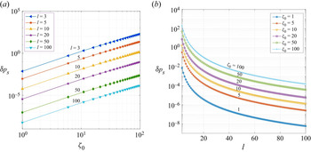
Note that we have assumed the presence of a pressure difference  $\delta p_s$ at the boundary,
 \begin{equation} \delta p_s ={-}\frac{3E_2}{2 l^4}\zeta_0^2 (3\cos^2\theta-1),\end{equation}
so that the boundary grains maintain the equilibrium structure based on the action–reaction law.
5. Results
5.1. Flow field: streamlines
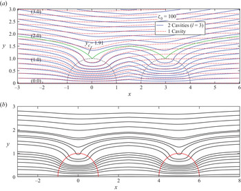
Examples of the flow field are given in figure 6.
Interaction of two cavities placed along the main flow ( $\zeta _0=100$): (a)
 $l=3$, where dotted lines are streamlines in the presence of a single cavity located at the same position as Cavity 1; and (b)
 $l=5$.

(i) In general, the velocity field is symmetric with respect to the mid-plane between the two cavities, as should be from the requirement of the geometry.
(ii) The flow field, however, has no fore-and-aft symmetry with respect to the perpendicular plane that passes through the centre of respective cavities. As is shown in figure 6(a), the streamlines of the rear side of Cavity 1 constrict toward the axis connecting the two cavities, whereas the opposite is the case with Cavity 2 that is located downstream of Cavity 1. For reference, streamlines for a single cavity (dotted lines) are superposed on those of Cavity 1 in figure 6(a). The constrictions of the streamlines in the rear side of Cavity 1, as shown in figure 6(a), however, become hardly recognizable in figure 6(b), where the centre-to-centre distance of the cavities amounts to approximately five times of its radius.
(iii) We can also recognize that the fluid volume flowing into Cavity 1 is larger than that for an isolated cavity, which reflects the fact that the two cavities (Cavity 1+Cavity 2) are regarded as the presence of an effectively larger cavity.
5.2. Velocity profile along the axis
5.2.1. Velocity $v_{x}$ along the axis

The velocity  $v_x$ along the axis of Cavity 1 is given by
 $$\begin{gather} v_x = 1- 2D\frac{1+\zeta_0 r}{r^3} \, \textrm{e}^{-\zeta_0 r} + 2E\left( \frac{1}{r^3}+\frac{1}{l^3} + \frac{3}{l^4} x \right), \quad (r \ge 1; \ x \le l/2), \end{gather}$$
 $$\begin{gather}v_x=Ar^2+B + 2Cx, \quad (r \le 1). \end{gather}$$
(1) Dependence of
$v_x$ on $\zeta _0$ for a fixed cavity distance $l$ is shown in figure 7(a). The velocity profile along the centreline of a single cavity, marked as $C_1$, is also plotted (dotted lines), which has fore-and-aft symmetry with respect to the perpendicular plane $\varSigma _1$ that passes the centre of Cavity 1. The magnitude of the latter (single cavity) increases with $\zeta _0$ until it reaches the speed six times of the undisturbed velocity. In the two-cavity case, however, the velocity field is not symmetric with respect to the plane $\varSigma _1$. In the cavity $C_1$, the velocity at the rear-side position is larger than that at its mirror image position at the front side.(2) The speed becomes maximum at the centre of the respective cavities, which increases with
$\zeta _0$. In contrast to the single cavity case, the maximum velocity exceeds 6 times of the undisturbed flow for the larger $\zeta _0$ case owing to the interaction of cavities.(3) The dependence of
$v_x$ on $l$ for fixed $\zeta _0$ is shown in figure 7(b). As $l$ increases, the velocity profile approaches the one that is piecewisely symmetric with respect to the plane $\varSigma _1$ or $\varSigma _2$.


Velocity along the axis of the cavities. (a) Dependence of  $v_x$ on
 $\zeta _0$, where the dotted lines are the velocity profile in the presence of a single cavity located at the position of Cavity 1. (b) Dependence of
 $v_x$ on
 $l$.

5.2.2. Velocity $v_{x}$ on the plane $x=\text {const.}$


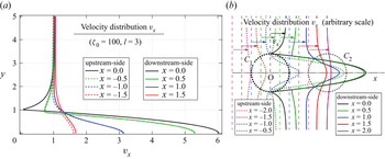
Figure 8 shows the velocity profiles at typical sections  $x = \textrm {const.}$ around Cavity 1. A closer look reveals that the magnitude of the velocity is larger in the downstream side than that of the upstream side. Owing to the cavity interaction, the velocity at the cavity centre can exceed six times of the undisturbed velocity for larger
 $\zeta _0$.
Velocity profile on the plane  $x= \textrm {const.}$ Dependence of
 $v_x$ at different positions of
 $x$: (a) comparison of upstream and downstream profiles for
 $l=3$; and (b) illustrative picture.

5.2.3. Stress distribution on the boundary
The negative normal stress distribution on the cavity boundary is of crucial importance to the collapse of the cavity, because granular boundaries are weak for negative normal stress (suction) while they are tough for positive normal stress (thrust) owing to the so-called ‘excluded volume effect’. For this reason, we focus our attention on the normal stress  $\tau _{rr}$. From (4.13), we have
 \begin{equation} \tau_{rr}^{(1)}={-}6A\cos\theta +2C(3\cos^2\theta -1), \end{equation}
on the boundary of the upstream-side of Cavity 1 and
 \begin{equation} \tau_{rr}^{(2)}={-}6A\cos\theta -2C(3\cos^2\theta -1), \end{equation}
on the boundary of the downstream-side of Cavity 2. The angles  $\theta$ and
 $\theta '$, which refer to respective cavity centres, are not distinguished unless otherwise stated.
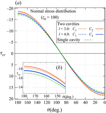
The dependence of  $\tau _{rr}$ on
 $\theta$ and
 $l$ is shown in figure 9. The result for a single cavity
 $(l \rightarrow \infty )$ is also shown. Figure 9 shows an example for
 $\zeta _0=100$, but the tendency is the same irrespective of the value
 $\zeta _0$. The latter can be seen from (5.2a) and (5.2b), because
 \begin{equation} {-}({\tau _{rr}}^{(2)} - {\tau _{rr}}^{(1)}) = 4C(3 \cos ^2 \theta - 1) = \frac{12E}{l^4}(3 \cos ^2 \theta - 1), \end{equation}
where
 \begin{equation} E = \frac{\varDelta_1}{\varDelta} = \left( 1 + \frac{30(1 + \zeta _0)}{\varDelta_1} - \frac{2}{l^3} \right)^{ - 1} \end{equation}
is a monotonically increasing function of  $\zeta _0 (\ge 0)$, whose minimum value
 $E_\textrm {min} = {(3 - 2/{l^3})}^{-1}$ is always positive for
 $l \ge 2$. The value of
 $- \tau _{rr}$ is largest at the front end of each cavity and it is larger for the downstream cavity. The difference, however, decreases as
 $l$ increases. These findings may explain why the downstream-side cavity is easily destroyed even when the upstream-side cavity keeps its structure, which will be further discussed in § 6.
Normal stress distribution on the cavity boundary. Panel (b), shown as the inset, is the close-up view of panel (a) near the front end of the cavity.

5.2.4. Variation of volume flux
For the two cavity case, the volumetric flow rate into Cavity 1 is given by the formula  $Q_{2c}= {\rm \pi}U_\infty y_{c}^{2}$, where
 $y_{c}$ is the distance from the
 $x$-axis after which the flow becomes almost uniform. We define the relative volumetric flow rate by
 \begin{equation} \Delta Q_{{Relative}}=\left(\frac{Q_{2c}-Q_{c}}{Q_{c}}\right)\times 100. \end{equation}
We observe that the volumetric flow rate into Cavity 1 increases for the two-cavity case compared with the single-cavity case. The increment may be attributed to the enhancement of the void region (rather relatively high permeable region) and the associated change in the flow field. We show the variation of  $Q_{{Relative}}$ for the case of two equally sized spherical cavities positioned in tandem (figure 10). The corresponding results for the 2-D case, as in Sano (Reference Sano2020), Kaneko & Sano (Reference Kaneko and Sano2003), are also shown. It is seen that the influence of the second cavity is felt when the centre-to-centre distance is within approximately seven times the radius of the cavity in a 3-D case with
 $\zeta _0 = 100$. It can be seen that
 $Q_{{Relative}}$ grows much faster in the 3-D case compared with the corresponding 2-D case as the cavities become closer. Figure 11(a) shows the dividing streamlines for different
 $l$. We see that the volume of the stream tube enclosing the shaded region that flows into the cavity increases as the centre-to-centre distance
 $l$ decreases. Figure 11(b) shows the dividing streamline for different
 $\zeta _{0}$. We see that as
 $\zeta _{0}$ increases, the volume of the stream tube enclosing the shaded region increases. As a result, the volumetric flow rate increases with
 $\zeta _{0}$.
Comparison of relative volume flux for two equally sized cavities positioned in tandem.

Dividing streamlines: (a) for different  $l$ when
 $\zeta _{0}=100;$ (b) for different
 $\zeta _{0}$ when
 $l=3$.

Figure 12 represents the axial velocity along the centreline for different  $\zeta _{0}$. We see that in the porous region, the distortion of the velocity takes place within a thin layer near the porous–liquid interface where the viscous forces (Brinkman) are effective, which is very often referred to as the Brinkman layer in the literature (see Le Bars & Worster Reference Le Bars and Worster2006; Hill & Straughan Reference Hill and Straughan2008). We see that in the Brinkman layer, the axial velocity undergoes an effect that is opposite to that in the cavity region. Inside this layer, increase of
 $\zeta _{0}$ reduces the velocity owing to the low permeability inside the porous region. However, away from this layer towards the interior of the cavity region, increase of
 $\zeta _{0}$ aids the velocity owing to the enhanced volumetric flow rate into the cavity (see figure 11). Beyond the Brinkman layer, however, the velocity is almost uniform (see figure 12).
Axial velocity along the centreline for different  $\zeta _{0}$.

5.3. Pressure difference as a function of $\zeta _0$

Figures 13(a) and 13(b) show the pressure difference at the boundary of Cavity 1 as a function of  $\zeta _0$ for fixed
 $l$ and as a function of
 $l$ for fixed
 $\zeta _0$, respectively. We see that the pressure difference increases with
 $\zeta _0$ for any
 $l$. This arises from the enhanced volumetric flow rate into the cavity for higher
 $\zeta _0$. However, the pressure difference increases rapidly with decrease of
 $l$ for any
 $\zeta _0$. Hence, two cavities situated at a shorter distance in the granular material with a higher
 $\zeta _0$ are more prone to collapse, which would give a clue to predict landslide and/or collapse of cliffs and river banks (irrespective of soils of different types).
Pressure difference at the boundary of the cavity as a function of (a)  $\zeta _{0}$ for different
 $l$, (b)
 $l$ for different
 $\zeta _{0}$.

6. Discussion
We have stated that the velocity at the centre of a single cavity  $V_c$ is enhanced, which amounts to three times and six times respectively for a circular cylindrical cavity (2-D case) and a spherical cavity (3-D case) of the undisturbed flow
 $U_\infty$, in a granular material with
 $\zeta _0 \gg 1$. What is the effect in the interacting cavities? To see this, the velocity at the centre of 2-D cavities positioned in tandem was reproduced (Sano Reference Sano2020), which is given explicitly by
 \begin{equation} \frac{V_c^{2D}}{U_\infty}=\frac{{\tilde D}_1}{{\tilde \varDelta}_2}, \end{equation}
where
 $$\begin{gather} {\tilde D}_1=\frac{1}{{\tilde \varDelta}_1}[8\zeta_0 K_0+(3\zeta_0^2+16)K_1], \quad {\tilde \varDelta}_2 =1-\frac{1}{l^2}\left(1-\frac{8K_1}{{\tilde \varDelta}_1}\right), \end{gather}$$
 $$\begin{gather}{\tilde \varDelta}_1=4\zeta_0 K_0+(\zeta_0^2+16)K_1, \quad K_0=K_0(\zeta_0), \quad K_1=K_1(\zeta_0), \end{gather}$$
and  $K_n$ is the modified Bessel function of order
 $n$. For 3-D spherical cavities positioned in tandem,
 $V_c^{3D}$ is given by
 \begin{equation} \frac{V_c^{3D}}{U_\infty}=B=\frac{3(2\zeta_0^3+7\zeta_0^2+15\zeta_0+15)}{\varDelta},\end{equation}
where
 \begin{align} \varDelta=\varDelta_0-\frac{2}{l^3}\varDelta_1, \quad \varDelta_0= \zeta_0^3+6\zeta_0^2+45\zeta_0+45, \quad \varDelta_1=\zeta_0^3+6\zeta_0^2+15\zeta_0+15. \end{align}
We show the dependence of  $V_c$ on
 $\zeta _0$ for fixed
 $l$ in figure 14. For
 $\zeta _0 \gg 1$, which is most likely encountered in groundwater flow, the velocity at the centre is given by
 \begin{equation} V_c^{2D} \sim \frac{3}{1-1/l^2} U_\infty, \quad V_c^{3D} \sim \frac{6}{1-2/l^3} U_\infty.\end{equation}
For the 3-D cases, interaction of cavities is larger in magnitude, but the influence decreases faster with the distance between the cavities.
Comparison of the velocity at the centre of 2-D and 3-D cavities.

If the far upstream velocity  $U_\infty$ exceeds a certain critical value
 $U_c$, a macroscopic cavity is destroyed by the enhanced stresses owing to the concentration of viscous flow into it. The criteria and the types of collapse that lead to the development of a fluidized region toward the upstream direction are fully elucidated by Kaneko & Sano (Reference Kaneko and Sano2005), Sano & Nagata (Reference Sano and Nagata2006) in 2-D cases. Presence of a second cavity of radius
 $R_2$ introduces further complication associated with their configuration, i.e. the ratio of two cavities
 $R_2/ R_0$, centre-to-centre distance between them
 $l$ (normalized by
 $R_0$) and the orientation of their alignment
 $\alpha$ with respect to the flow at infinity. Even in the simplest case of two equally sized cavities (
 $R_2=R_0$) in a given material (
 $\zeta _0$ fixed), the onset of collapse
 $U_c$ and the processes that follow depend on
 $l$ and
 $\alpha$. By systematic experiments, the types of collapse (no collapse, partial collapse, ‘stick–slip’ collapse and ‘complete’ collapse) based on
 $l, \alpha$ and
 $U^*~(=U_{\infty }/U_{c})$ are found, as reported by Kaneko & Sano (Reference Kaneko and Sano2005). Generally speaking, cavities collapse completely and independently for
 $U^* \gg 1$, if they are sufficiently far apart from each other, or if they are not so distant to each other but arranged spanwise (i.e.
 $\alpha \approx 90^{\circ }$). However, if the two cavities are close enough and
 $\alpha$ is not so large, they migrate toward the upstream direction (Sano Reference Sano2011) or merge to form a longer fluidized region (see Kaneko & Sano Reference Kaneko and Sano2005; Sano & Nagata Reference Sano and Nagata2006) that extends almost along the flow direction. The size and the temporal behaviour of the fluidized region depend on the configuration
 $l, \alpha$ and
 $U^*$. It should be noted that the downstream cavity positioned in tandem with smaller
 $l$ collapses even under subcritical magnitude
 $U_c$ (see Kaneko & Sano Reference Kaneko and Sano2003, Reference Kaneko and Sano2005) and merges with the upstream cavity, because a stronger stream focused by the upstream cavity is released downstream. This phenomenon is in strong contrast to our daily-life experience where the flow is weaker behind solid objects. These processes are also reproduced by their numerical simulation. As far as the initial stage of collapse is concerned, theoretical analysis is made by taking into account the asymptotic effect of the other cavity and the configuration of the two cavities that is most easily damaged (see Sano Reference Sano2020). Similar situations are observed in the present 3-D interacting cavities. To see this, let us compare
 $\tau _{rr}$ for a single spherical cavity given by (3.11a) with that of two cavities given by (5.2a,b). As mentioned before, the most vulnerable position is the upstream end of a single spherical cavity, as well as the upstream ends of the respective spherical cavities positioned in tandem. For a single spherical cavity, normal stress is
 \begin{equation} \tau_{rr}(r=1, \theta={\rm \pi})=6A_1={-}\frac{18\zeta_0^2 (1+\zeta_0)}{\varDelta_0} \equiv{-} S_0, \end{equation}
while for two spherical cavities positioned in tandem, they are
 \begin{equation} \tau_{rr}^{(1)}(r=1, \theta={\rm \pi})=6A+4C ={-}\frac{18}{\varDelta}\left(\zeta_0^2 (1+\zeta_0)-\frac{2\varDelta_1}{3l^4}\right) \equiv{-} S_1 \end{equation}
and
 \begin{equation} \tau_{rr}^{(2)}(r=1, \theta={\rm \pi})=6A-4C ={-}\frac{18}{\varDelta}\left(\zeta_0^2 (1+\zeta_0)+\frac{2\varDelta_1}{3l^4}\right) \equiv{-} S_2, \end{equation}
for cavities  $C_1$ and
 $C_2$, respectively. The differences of the negative normal stresses between them are
 \begin{equation} S_1-S_0=\frac{12\varDelta_1}{l^3 \varDelta}\left(\frac{3\zeta_0^2 (1+\zeta_0)}{\varDelta_0} -\frac{1}{l}\right),\end{equation}
and
 \begin{equation} S_2-S_0=\frac{12\varDelta_1}{l^3 \varDelta}\left(\frac{3\zeta_0^2 (1+\zeta_0)}{\varDelta_0} +\frac{1}{l}\right).\end{equation}
In accordance with those described in § 5.3,  $S_2-S_1=8C>0$, the downstream side cavity
 $C_2$ is always exposed to a stronger stream than the upstream cavity
 $C_1$. From (6.8b), we have
 $S_2 > S_0$, so that the front end of the downstream cavity
 $C_2$ always undergoes a stronger suction force than the single cavity. However,
 $S_1 > S_0$ holds for the case
 \begin{equation} l > \frac{\varDelta_0}{3\zeta_0^2 (1+\zeta_0)} \equiv l_c, \end{equation}
so that the front end of the upstream cavity  $C_1$ undergoes a stronger suction force than the single cavity. The latter may be attributed to the emergence of effectively larger cavities owing to the presence of two cavities, which accelerates the flow near the axis. However, the relation
 $S_1 < S_0$ holds for the case
 $l < l_c$, so that under subcritical condition where a single spherical cavity collapses, it happens that the upstream cavity
 $C_1$ remains stable while the downstream cavity
 $C_2$ collapses. Quantitative estimation of the critical distance will require further analysis by considering the interaction of cavities closer to each other. The deformation of void space in a rock (see Davis et al. Reference Davis, Healy, Bubeck and Walker2017) has remarkable resemblance to the cavity collapse in granular material, whose mechanisms seem common to each other. In the former, compressive stress is the principal control parameter for rock fractures, so that the pole region (far end regions along the applied compressive stress direction) is flattened and the side region (equatorial region) is elongated. However, suction force or tensile stress is the principal control parameter for the collapse of a cavity region exposed to fluid flow. Here the positions of ‘poles’ in the rock fracture mechanism correspond to the upstream-end and/or downstream-end of the cavity. In general, compressive stress gives tensile stress to the perpendicular direction, so that their results, i.e.: (i) pole region of the spherical (or circular) void is flattened, while side region is elongated; (ii) oblate spheroidal void (whose axis is along the compressive stress) is deformed easier than prolate spheroidal void; (iii) interaction of two circular voids under compressive stress (that leads to coalescence) is larger for voids that lie in orientations approximately perpendicular to the applied stress, etc., qualitatively agree with our case, by replacing ‘compressive stress’ with ‘tensile stress’ in the direction perpendicular to the former. Although we have not shown the result ii) of Davis et al. (Reference Davis, Healy, Bubeck and Walker2017) in this paper, our previous 2-D studies (see Raja Sekhar & Sano Reference Raja Sekhar and Sano2003; Kaneko & Sano Reference Kaneko and Sano2005; Sano & Nagata Reference Sano and Nagata2006; Sano Reference Sano2020) agree with them in that an elliptic cylindrical cavity or two circular cylindrical cavities along the stream (approximately equivalent to the oblate spheroid in the configuration of Davis et al. (Reference Davis, Healy, Bubeck and Walker2017)) is easier to collapse than those across the stream (approximately equivalent to the prolate spheroid).
In the presence of distributed cavities, a macroscopically connected fluidized region, such as a long channel, network and sheet-like region, can be created through repeated collapse and merging of cavities, which can be a trigger of the landslides and/or the collapse of river banks (see Sano Reference Sano2011). A similar situation is anticipated in human tissues and organs. For example, the histological anatomy of the liver lobule shows that our human liver consists of globular cells surrounding the portal triad (portal vein, hepatic artery and bile ductule). A sinusoid is a narrow space or passage for blood in this tissue, analogous to the interstices between the grains of a granular material. In normal conditions, these sinusoids are highly connected, but the connectedness of the passage (closely related with permeability) decreases in cirrhosis and is sparsely connected in cancer. In fact, the connectedness of the passage, characterized by the ‘1st Betti number’ are reported as 181, 85 and 47 for normal, cirrhosis and cancer in the examined tissue,  $200\times 200\times 80\ \mathrm {\mu }\textrm {m}^3$ in size, (see Shimizu & Yokoyama Reference Shimizu and Yokoyama1993; Shimizu, Suda & Yokoyama Reference Shimizu, Suda and Yokoyama1996; Shimizu Reference Shimizu2012). From the analogy between granular material and the liver tissue, the formation of a water channel in the former corresponds to the creation of a new passage of blood flow (angiogenesis) in a diseased liver. When some tumour cells grow quickly, the volumetric flow rate into that part is enhanced. As a result, a specific blood vessel is expected to provide larger volumetric flow rate (see Sano Reference Sano2008). In this context, one may note that targeted drug therapy for treating cancer, diabetes and atherosclerosis is becoming popular. In such kinds of illness, liposomes (nanoscale molecules made of a lipid bilayer) that contain important medication can be easily transported to a targeted cell by using the improved blood stream (see Waite & Roth Reference Waite and Roth2012). However, when some part of the organ is cemented and permeability is lowered, then blood flow can be initiated to transport liposomes with a drug by putting a small hole in the proximity of that low permeability region. In such scenarios, the arrangement of the ‘cavities’ plays an important role to achieve maximum volumetric flux, which could develop a new blood vessel. The latter may become a useful medical engineering technique in the future. The present 3-D analysis will provide more realistic foundations to these interdisciplinary applications.
7. Conclusions
Three-dimensional flow of an incompressible viscous fluid in the presence of macroscopic cavities is analysed. The fluid flow inside the cavities is governed by Stokes equation and the flow outside the cavities by Darcy–Brinkman equation. Interactions of two cavities with centre-to-centre distance  $l$ in a uniform stream at infinity are investigated by assessing the asymptotic impact of Darcylet owing to the other cavity. Present analysis shows that the volumetric flow rate is enhanced when the centre-to-centre distance
 $l$ is reduced. We have shown that the volume flux at
 $l =3$ amounts to as large as 3.65 times of that flowing through the same sufficiently large granular material without cavities. This amounts to the enhancement of the relative volumetric flux by
 $22\,\%$ compared with that observed for a single cavity. The increment becomes larger as
 $\zeta _0$ increases. The local velocity is also enhanced with the decrease of
 $l$. The velocity at the centre of the cavity amounts to 6.48 times of the undisturbed flow at
 $l =3$, which is
 $8\,\%$ larger than that observed for a single cavity. The increment of velocity becomes larger as
 $\zeta _0$ increases. We have also shown that the enhancement of the volume flux increases the local stresses at the boundary of cavities, whose magnitude becomes larger as the distance
 $l$ is reduced. The enhancement of stresses is larger for a granular material having higher
 $\zeta _0$.
Owing to the local enhancement of volume flux into the cavity, it becomes prone to collapse. It is shown that two cavities situated at a fixed distance are more prone to collapse for a granular material having higher  $\zeta _0$. These findings help us to understand the network formation of groundwater in the soil and hence to predict landslides and collapse of banks. The experimental investigations are limited to 2-D situations; however, in numerous real-life situations, cavities are more often three-dimensional. The present study provides a more comprehensive understanding on the interaction of cavities and provides clues to predict the collapse for a three-dimensional scenario.
Acknowledgements
We thank the reviewers for their valuable comments and suggestions which resulted in the improvement of the manuscript.
Funding
This research received no specific grant from any funding agency, commercial or not-for-profit sectors.
Declaration of interests
The authors report no conflict of interest.
Author contributions
O.S. analysed the preliminary part of this problem, which was presented at the Stokes200 Symposium held at Cambridge 2019 and also contributed to numerical results, analysis and the drafting of the manuscript. T.K. performed numerical results, analysis and contributed in the drafting of the manuscript. G.P.R.S. contributed to mathematical analysis, verifying the numerical results and completing the manuscript. All authors read and approved the manuscript.
Appendix A. Solution of (2.6) (2.7) with (2.4)
Taking the divergence of (2.6) and using (2.4), we have  $\Delta p=(\boldsymbol {F} \boldsymbol {\cdot }\boldsymbol {\nabla })\delta (\boldsymbol {r}).$ The particular solution
 $p$ is given by
 \begin{equation} p=\left(\boldsymbol{F} \boldsymbol{\cdot} \boldsymbol{\nabla}\right)\phi_{0}(\boldsymbol{r}), \quad \textrm{where}\ \Delta \phi_{0}(\boldsymbol{r})=\delta(\boldsymbol{r}) \quad \textrm{or} \quad \phi_{0}={-}\frac{1}{4 {\rm \pi}r}. \end{equation}
Thus we have
 \begin{equation} p=\frac{\boldsymbol{F}\boldsymbol{\cdot} \boldsymbol{r}}{4 {\rm \pi}r^{3}}.\end{equation}
Substitution of (A 2) into (2.6) yields
 \begin{equation} (\varDelta-\zeta_{0}^{2}) \boldsymbol{v}=(\boldsymbol{F}\boldsymbol{\cdot} \boldsymbol{\nabla})\boldsymbol{\nabla} \phi_{0}(\boldsymbol{r})-\boldsymbol{F} \delta(\boldsymbol{r}). \end{equation}
We put  ${\boldsymbol v}={\boldsymbol v}_1+{\boldsymbol v}_2$, such that
 \begin{equation} (\varDelta - \zeta_0^2) {\boldsymbol{v}}_1={-} {\boldsymbol F}\delta(\boldsymbol{r}), \quad (\varDelta - \zeta_0^2) {\boldsymbol{v}}_2 = ({\boldsymbol F}\boldsymbol{\cdot} \boldsymbol{\nabla})\boldsymbol{\nabla} \phi_0(\boldsymbol{r}).\end{equation}
The solution of (A4) is given by  ${\boldsymbol v}_1= - {\boldsymbol F} \phi _\zeta,$ where
 \begin{equation} (\varDelta - \zeta_0^2) \phi_\zeta=\delta(\boldsymbol{r}) \quad \textrm{or}\quad \phi_\zeta={-}\frac{ \textrm{e}^{-\zeta_0 r}}{4{\rm \pi} r}. \end{equation}
In terms of  $\tilde {\phi }$ that satisfies
 $(\varDelta - \zeta _0^2) \tilde {\phi } =\phi _0$, we obtain
 ${\boldsymbol v}_2=({\boldsymbol F}\boldsymbol {\cdot } \boldsymbol {\nabla })\boldsymbol {\nabla } \tilde {\phi }.$ Here
 $$\begin{gather} (\varDelta - \zeta_0^2) \phi_0=\Delta \phi_0 - \zeta_0^2 \phi_0=\delta(\boldsymbol{r}) - \zeta_0^2 \phi_0 =(\varDelta - \zeta_0^2) \phi_\zeta - \zeta_0^2 \phi_0, \end{gather}$$
 $$\begin{gather}(\varDelta - \zeta_0^2) (\phi_\zeta-\phi_0)= \zeta_0^2 \phi_0 \rightarrow \tilde{\phi}=\frac{\phi_\zeta-\phi_0}{\zeta_0^2}, \end{gather}$$
so that
 \begin{equation} {\boldsymbol v}_2=({\boldsymbol F}\boldsymbol{\cdot} \boldsymbol{\nabla})\boldsymbol{\nabla} \tilde{\phi} =\frac{1}{\zeta_0^2} ({\boldsymbol F}\boldsymbol{\cdot} \boldsymbol{\nabla})\boldsymbol{\nabla} (\phi_\zeta-\phi_0). \end{equation}
Direct calculation of  $\boldsymbol {v}_{1}+\boldsymbol {v}_{2}$, using
 $\phi _{0}$ and
 $\phi _{\zeta }$, yields (2.8).