1. Introduction
Liquid jets can be formed in a multitude of ways by free-surface flows. Fluid is often forced through nozzles to generate jets and drops in a controlled manner, as in a kitchen tap or ink-jet printing. Hydrostatic or capillary pressure can also lead to jet formation when an air cavity is formed on a free surface by an impacting object (Worthington & Cole Reference Worthington and Cole1897, Reference Worthington and Cole1900; Gekle et al. Reference Gekle, Gordillo, van der Meer and Lohse2009) or when a bursting bubble collapses at an interface and focuses a jet of liquid upwards (Boulton-Stone & Blake Reference Boulton-Stone and Blake1993; Duchemin et al. Reference Duchemin, Popinet, Josserand and Zaleski2002). Other drivers of jet formation include Faraday waves when the vibration amplitude exceeds a critical value (Zeff et al. Reference Zeff, Kleber, Fineberg and Lathrop2000), surface acoustic waves that refract into a drop and generate flow through acoustic streaming (Tan, Friend & Yeo Reference Tan, Friend and Yeo2009), pressure waves from the impact of a tube filled with a liquid (Antkowiak et al. Reference Antkowiak, Bremond, Le Dizes and Villermaux2007), and laser pulses focused in a liquid, which leads to an expanding vapour cavity (Blake & Gibson Reference Blake and Gibson1987; Duocastella et al. Reference Duocastella, Fernández-Pradas, Morenza and Serra2009; Tagawa et al. Reference Tagawa, Oudalov, Visser, Peters, van der Meer, Sun, Prosperetti and Lohse2012; Peters et al. Reference Peters, Tagawa, Oudalov, Sun, Prosperetti, Lohse and van der Meer2013; Patrascioiu et al. Reference Patrascioiu, Fernández-Pradas, Palla-Papavlu, Morenza and Serra2014).
In this paper, we analyse the early-time dynamics of a different method for jet formation, motivated by a novel process for printing called blister-actuated laser-induced forward transfer (BA-LIFT) (Brown, Kattamis & Arnold Reference Brown, Kattamis and Arnold2010; Brown et al. Reference Brown, Brasz, Ventikos and Arnold2012). We focus on the fluid dynamics and are concerned with jet formation from a layer of fluid that is set in motion by the rapid deformation of part of a solid boundary. An initially flat boundary changes shape, forming a bump and transferring momentum to the fluid. If this momentum is large enough to overcome surface tension and gravitational forces, a jet will form in the same direction as the bump.
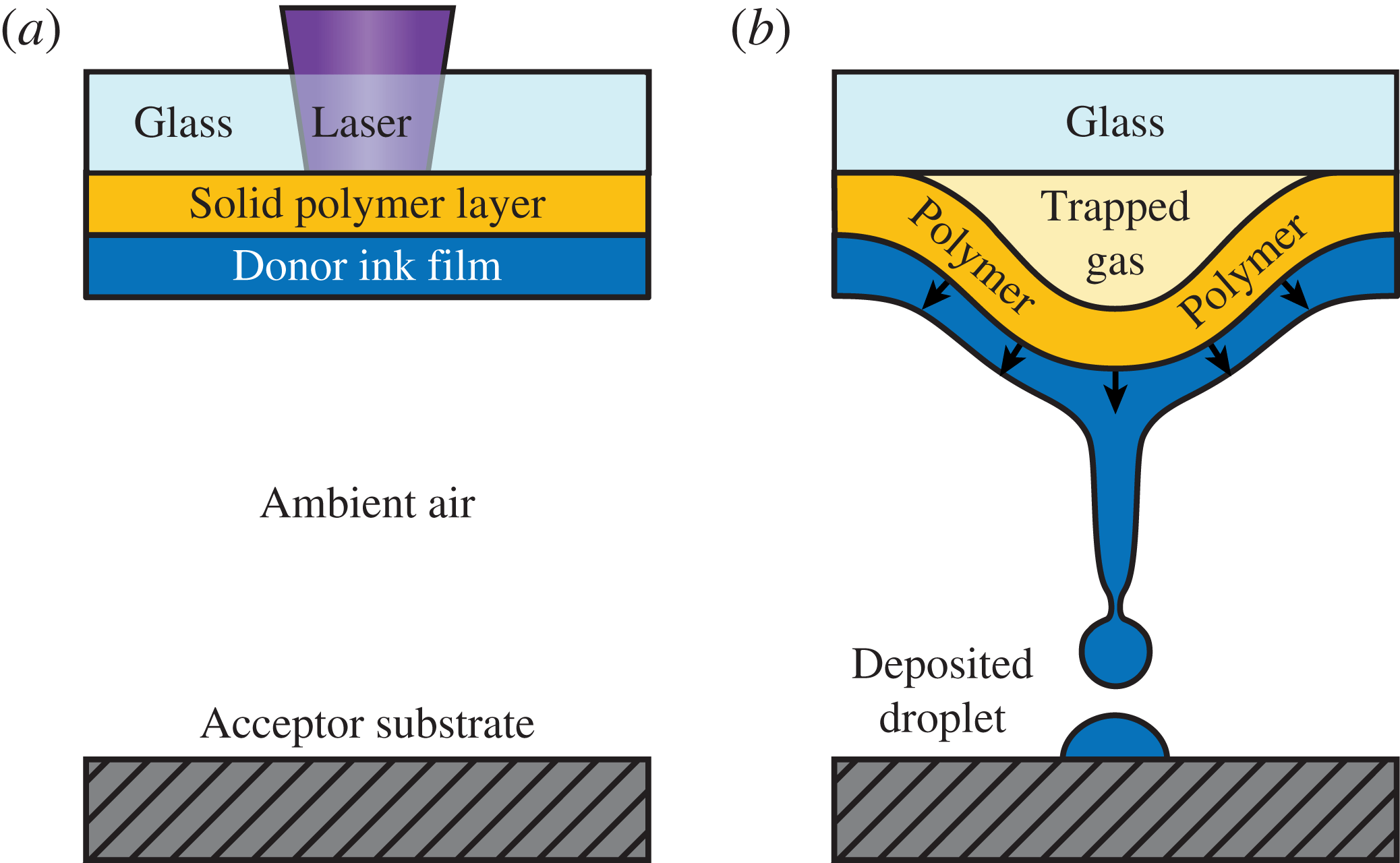
In the process of BA-LIFT, the deformation of the boundary is achieved by the absorption of a laser pulse. The pulse is focused through a glass slide, ablating a confined region of a polymer film, which subsequently expands as a sealed vapour cavity to produce a blister (see figure 1). The blister formation initiates the transfer of material from a donor film of liquid to an acceptor substrate in the form of a liquid jet.
Blister-actuated laser-induced forward transfer. (a) A laser pulse is absorbed within a thin polymer layer, which is coated with a liquid film of ink. (b) Vaporization produces a sealed gas cavity that rapidly pushes the polymer film away from the glass as a blister. A liquid jet is formed if the impulse from the blister is strong enough, and ink is transferred to an acceptor substrate.

BA-LIFT is one of many variations of laser-induced forward transfer (LIFT), which all have in common that a laser pulse is focused through a transparent substrate into a thin film of donor material, propelling the material to an acceptor substrate a fixed distance away. LIFT offers an alternative to nozzle-based techniques such as ink-jet printing in which clogging and material compatibility issues can be restrictive (Bohandy, Kim & Adrian Reference Bohandy, Kim and Adrian1986; Kyrkis et al. Reference Kyrkis, Andreadaki, Papazoglou and Zergioti2006; Arnold, Serra & Piqué Reference Arnold, Serra and Piqué2007). LIFT has been demonstrated as an effective method for printing cells in tissue engineering applications (Ringeisen et al. Reference Ringeisen, Othon, Barron, Young and Spargo2006; Schiele et al. Reference Schiele, Corr, Huang, Raof, Xie and Chrisey2010; Koch et al. Reference Koch, Deiwick, Schlie, Michael, Gruene, Coger, Zychlinski, Schambach, Reimers, Vogt and Chichkov2012), biomaterials for biosensors and drug-delivery systems (Palla-Papavlu et al. Reference Palla-Papavlu, Paraico, Shaw-Stewart, Dinca, Savopol, Kovacs, Lippert, Wokaun and Dinescu2011) and semiconducting materials for organic electronics (Shaw-Stewart et al. Reference Shaw-Stewart, Mattle, Lippert, Nagel, Nüesch and Wokaun2013; Zergioti Reference Zergioti2013). In the standard application of LIFT, the laser pulse irradiates a metal absorbing layer to form a bubble in the adjacent liquid film and a liquid jet forms on this bubble. BA-LIFT offers an advantage over the standard approach by converting the thermal impulse of the laser pulse into a mechanical impulse through the use of a thicker polymer layer, which allows thermally sensitive materials such as stem cells (Kattamis et al. Reference Kattamis, Purnick, Weiss and Arnold2007) and luminophores for organic electronics (Kattamis et al. Reference Kattamis, McDaniel, Bernhard and Arnold2009, Reference Kattamis, McDaniel, Bernhard and Arnold2011) to be transferred safely, insulated from the extreme heat of a laser pulse.
The mechanisms behind jet formation in LIFT have been investigated with experimental time-resolved imaging (Duocastella et al. Reference Duocastella, Fernández-Pradas, Morenza and Serra2009; Brown, Kattamis & Arnold Reference Brown, Kattamis and Arnold2011; Brasz, Yang & Arnold Reference Brasz, Yang and Arnold2015; Patrascioiu et al. Reference Patrascioiu, Fernández-Pradas, Palla-Papavlu, Morenza and Serra2014) and numerical simulations (Brown et al. Reference Brown, Brasz, Ventikos and Arnold2012), but open questions remain in understanding the underlying fluid dynamics. In BA-LIFT particularly, how does the finite deformation of a boundary lead to a jet-forming flow? For how long does the fluid remain in motion after the blister expansion stops?
Numerical simulations reveal that in the blister expansion process only a small fraction of the initial kinetic energy transferred to the fluid remains after the blister stops expanding (Brown et al. Reference Brown, Brasz, Ventikos and Arnold2012). Moreover, the initial velocity field is directed radially outwards from the expanding blister, whereas the velocity field after the blister has finished expanding is radially inwards, pulling fluid in to form a jet. We seek to quantitatively understand the energy transfer and flow reversal due to a deforming solid boundary, as they are both crucial to jet formation.
In this paper, a domain-perturbation technique is used in the limit of shallow solid boundary deformations to solve for the time-dependent fluid flow as the boundary deforms. By ‘shallow’, we mean that the ratio of boundary deformation height
 $H_{b}$
to radius
 $R_{b}$
is small. For the majority of the paper, we assume a two-dimensional domain with a sinusoidal deformation of a solid boundary in order to keep the algebra simpler and make the physical ideas clearer, so the actual problem being solved is the flow field due to the formation of a spatially periodic array of bumps. The extension to an axisymmetric domain with a Gaussian deformation will be presented afterwards and shown to exhibit the same qualitative flow features.
The time scale of the boundary deformation in BA-LIFT (
 ${\sim}30~\text{ns}$
) is very much smaller than the relevant capillary, viscous and gravitational time scales (all
 ${\gtrsim}10~{\rm\mu}\text{s}$
), so the induced flow is primarily inertial and the effects of surface tension, viscosity and gravity can be neglected initially. Capillary forces eventually become important, driving pinch-off, but the disparity in time scales allows the problem to be separated into an inertial energy transfer from the blister to the fluid at early times and the formation of a jet and drops at longer times.
The formulation of the problem, non-dimensionalization and examination of time scales are presented in § 2. In § 3, we introduce the domain-perturbation technique and present the solution; the fluid flow stops with the motion of the solid boundary in the first-order solution, so the second-order solution is obtained as well. In § 4, a particular time dependence is assumed for the boundary deformation, allowing for a discussion of the resulting velocity field and free-surface evolution. In § 5, we integrate the kinetic energy in the fluid, revealing a transition from the initial impulsive energy to the remnant energy after the boundary deformation slows. In § 6, the domain-perturbation calculation is extended to an axisymmetric domain with a Gaussian boundary deformation. In § 7, we explore the applicability of the asymptotic theory with finite-difference simulations of the free-surface potential flow. In § 8, we discuss implications of the results for BA-LIFT, obtaining an estimate for the threshold laser pulse energy for pinch-off of a drop. We conclude with a discussion of the results in § 9.
2. Mathematical formulation
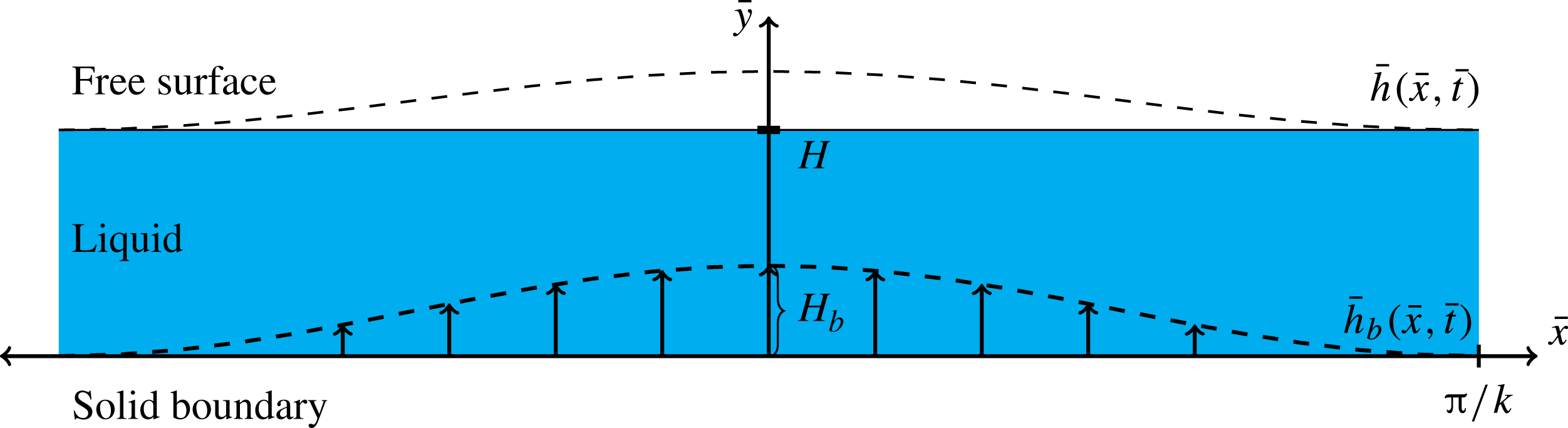
We consider a liquid with density
 ${\it\rho}$
initially at rest in a horizontal layer
 $0<\bar{y}<H$
with a solid boundary at
 $\bar{y}=0$
and a free surface at
 $\bar{y}=H$
(see figure 2). We neglect any effects of the ambient air, which is at constant pressure. The spatially periodic deformation of the solid boundary is given by prescribing a vertical velocity
 $$\begin{eqnarray}\bar{V}_{b}(\bar{x},\bar{t})={\textstyle \frac{1}{2}}(1+\cos k\bar{x})\,\bar{f}(\bar{t}),\end{eqnarray}$$
with an arbitrary time dependence
 $\bar{f}(\bar{t})$
; the factor of
 $1/2$
is included for convenience later. We define
 $\bar{F}(\bar{t})\equiv \int _{0}^{\bar{t}}\bar{f}(s)\text{d}s$
, so that the vertical displacement of the boundary is
 $$\begin{eqnarray}\bar{h}_{b}(\bar{x},\bar{t})={\textstyle \frac{1}{2}}(1+\cos k\bar{x})\bar{F}(\bar{t}).\end{eqnarray}$$
We will consider a boundary deformation that approaches a maximum equilibrium displacement
 $H_{b}$
; i.e.
 $\lim _{\bar{t}\rightarrow \infty }\bar{F}(\bar{t})=H_{b}$
. We note, however, that the results will apply for arbitrary
 $\bar{F}(\bar{t})$
for most of the calculation, so the analysis could also be used for a boundary oscillating in time, for example.
Diagram of the problem set-up.

The boundary deformation induces a fluid flow with velocity
 $\bar{\boldsymbol{u}}$
and pressure
 $\bar{p}$
. As the fluid is initially at rest and assumed to be inviscid, the flow will remain irrotational throughout the boundary deformation, and a velocity potential
 $\bar{{\it\phi}}(\bar{x},\bar{y},\bar{t})$
defined as
 $\boldsymbol{{\rm\nabla}}\bar{{\it\phi}}=\bar{\boldsymbol{u}}$
can be used. The governing equations are then continuity,
 $\boldsymbol{{\rm\nabla}}\boldsymbol{\cdot }\bar{\boldsymbol{u}}=0$
, and the unsteady Bernoulli equation, or
 $$\begin{eqnarray}\displaystyle & {\rm\nabla}^{2}\bar{{\it\phi}}=0, & \displaystyle\end{eqnarray}$$
 $$\begin{eqnarray}\displaystyle & \displaystyle \frac{\partial \bar{{\it\phi}}}{\partial \bar{t}}+\frac{1}{2}(\bar{u}^{2}+\bar{v}^{2})+\frac{\bar{p}}{{\it\rho}}=0, & \displaystyle\end{eqnarray}$$
 $\partial \bar{{\it\phi}}/\partial \bar{t}$
.
At the solid wall, the kinematic boundary condition is
 $$\begin{eqnarray}\bar{V}_{b}(\bar{x},\bar{t})+\bar{u}\frac{\partial \bar{h}_{b}}{\partial \bar{x}}\bigg|_{\bar{y}=\bar{h}_{b}}=\bar{v}|_{\bar{y}=\bar{h}_{b}}.\end{eqnarray}$$
Letting
 $\bar{h}(\bar{x},t)$
denote the height of the free surface, the kinematic boundary condition there is
 $$\begin{eqnarray}\frac{\partial \bar{h}}{\partial \bar{t}}+\bar{u}\frac{\partial \bar{h}}{\partial \bar{x}}\bigg|_{\bar{y}=\bar{h}}=\bar{v}|_{\bar{y}=\bar{h}},\end{eqnarray}$$
with an initial condition of
 $\bar{h}(\bar{x},0)=H$
. The pressure is constant at the free surface and can be set to 0. Applying (2.3b
), we obtain the dynamic boundary condition
 $$\begin{eqnarray}\left.\frac{\partial \bar{{\it\phi}}}{\partial \bar{t}}\right|_{\bar{y}=\bar{h}}=-\frac{1}{2}(\bar{u}^{2}+\bar{v}^{2})_{\bar{y}=\bar{h}}.\end{eqnarray}$$
The mathematical problem is to solve (2.3a
) subject to the boundary conditions (2.4)–(2.6). The flow is driven by the boundary deformation,
 $h_{b}(x,t)$
, given in (2.2). In particular, we are interested in the velocity field and free-surface motion as the solid boundary approaches a steady state.
2.1. Non-dimensionalization
We non-dimensionalize lengths and times by the inverse wavenumber of the boundary deformation,
 $k^{-1}$
, and the characteristic time for boundary deformation,
 ${\it\tau}$
, respectively, which results in a characteristic speed
 $(k{\it\tau})^{-1}$
. This step allows us to write
 $x=k\bar{x}$
,
 $y=k\bar{y}$
,
 $t=\bar{t}/{\it\tau}$
,
 $u=k{\it\tau}\bar{u}$
,
 $v=k{\it\tau}\bar{v}$
,
 ${\it\phi}=k^{2}{\it\tau}\bar{{\it\phi}}$
,
 $h=k\bar{h}$
,
 $h_{b}=k\bar{h}_{b}$
,
 $V_{b}=k{\it\tau}\bar{V}_{b}$
and
 $p=(k{\it\tau})^{2}\bar{p}/{\it\rho}$
, where
 $x$
,
 $y$
,
 $t$
,
 $u$
,
 $v$
,
 ${\it\phi}$
,
 $h$
,
 $h_{b}$
,
 $V_{b}$
and
 $p$
are all dimensionless quantities. For the boundary velocity and displacement, we write the time dependence in the form
 $$\begin{eqnarray}f(t)=\frac{\bar{f}(\bar{t})}{H_{b}/{\it\tau}},\quad F(t)=\frac{\bar{F}(\bar{t})}{H_{b}},\end{eqnarray}$$
so that
 $\lim _{t\rightarrow \infty }F(t)=1$
and
 $\lim _{t\rightarrow \infty }f(t)=0$
. The dimensionless boundary velocity and displacement then become
 $$\begin{eqnarray}V_{b}(x,t)={\it\epsilon}(1+\cos x)\,f(t),\quad h_{b}(x,t)={\it\epsilon}(1+\cos x)F(t),\end{eqnarray}$$
where
 ${\it\epsilon}\equiv kH_{b}/2$
is a dimensionless parameter that describes the aspect ratio of the boundary deformation. Note that, by defining a typical blister radius
 $R_{b}\equiv {\it\lambda}/2$
in terms of the wavelength
 ${\it\lambda}\equiv 2{\rm\pi}/k$
, the aspect ratio can be written as
 ${\it\epsilon}={\rm\pi}H_{b}/2R_{b}$
.
The other dimensionless parameter is
 ${\it\beta}\equiv kH$
, which measures the ratio of the initial layer thickness to the wavelength of the boundary deformation and appears in the initial condition for the interfacial height,
 $h(x,0)={\it\beta}$
. Figure 2 illustrates the set-up for
 ${\it\epsilon}=0.2$
and
 ${\it\beta}=1$
, which are typical values for BA-LIFT experiments.
2.2. Effects of surface tension and viscosity at early times
We briefly examine the assertion made in § 1 that surface tension
 ${\it\gamma}$
, viscosity
 ${\it\mu}$
and gravity can be neglected in the early-time dynamics of BA-LIFT. The liquid used in the experiments and considered in the numerical simulations of Brown et al. (Reference Brown, Brasz, Ventikos and Arnold2012) was
 $N$
-methyl-2-pyrrolidone (NMP), which has
 ${\it\gamma}=40.8~\text{mN}~\text{m}^{-1}$
,
 ${\it\rho}=1030~\text{kg}~\text{m}^{-3}$
and
 ${\it\mu}=1.7~\text{mPa}~\text{s}$
. Taking
 $R_{b}\approx 20~{\rm\mu}\text{m}$
as a typical deformation length scale,
 $H\approx 5~{\rm\mu}\text{m}$
as a viscous and gravitational length scale, and the fluid properties of NMP, we can define the capillary, viscous and gravitational time scales as
 $$\begin{eqnarray}t_{cap}=\sqrt{{\it\rho}R_{b}^{3}/{\it\gamma}}\approx 14~{\rm\mu}\text{s},\quad t_{{\it\nu}}=H^{2}/{\it\nu}\approx 15~{\rm\mu}\text{s},\quad t_{g}=\sqrt{H/g}\approx 700~{\rm\mu}\text{s},\end{eqnarray}$$
with
 ${\it\nu}={\it\mu}/{\it\rho}$
and
 $g=9.81~\text{m}~\text{s}^{-2}$
. Compared with the characteristic time for blister formation,
 ${\it\tau}\approx 37~\text{ns}$
, these time scales are at least a factor of 300 larger, justifying our subdivision of the jet formation process. At early times (
 $t=\bar{t}/{\it\tau}\lesssim 10$
), the deformation of the solid boundary induces an inertial flow initiating jet formation; and at later times, the effects of surface tension and possibly viscosity become important during jet growth and pinch-off into drops.
3. Domain perturbation
For an arbitrary value of
 ${\it\epsilon}$
, the nonlinear boundary conditions and significantly changing domain shape prevent complete solution by analytical means. For small
 ${\it\epsilon}$
, however, the domain-perturbation technique (e.g. van Dyke Reference van Dyke1964) can be used to obtain an approximate solution via asymptotic expansions. In the domain-perturbation problem, both the solution within the domain and the boundaries of the domain are represented as asymptotic expansions in
 ${\it\epsilon}$
. For small
 ${\it\epsilon}$
, the boundaries of the actual time-dependent fluid domain are only slightly perturbed from those of the original undeformed rectangular domain. It is thus possible to use Taylor series to represent the values needed at the actual boundary positions in terms of values at the nearby original boundary positions. By this means the full nonlinear problem on the deformed domain can be transformed into a series of linear problems, at successive powers of
 ${\it\epsilon}$
, on the original undeformed domain.
For the potential
 ${\it\phi}$
, we write
 $$\begin{eqnarray}{\it\phi}(x,y,t;{\it\epsilon})={\it\epsilon}{\it\phi}_{1}(x,y,t)+{\it\epsilon}^{2}{\it\phi}_{2}(x,y,t)+\cdots \,,\end{eqnarray}$$
where
 ${\rm\nabla}^{2}{\it\phi}_{i}=0$
for all
 $i$
. Since
 $\boldsymbol{u}=\boldsymbol{{\rm\nabla}}{\it\phi}$
, it follows that
 $$\begin{eqnarray}u(x,y,t;{\it\epsilon})=\mathop{\sum }_{i=1}^{\infty }{\it\epsilon}^{i}u_{i}(x,y,t),\quad v(x,y,t;{\it\epsilon})=\mathop{\sum }_{i=1}^{\infty }{\it\epsilon}^{i}v_{i}(x,y,t).\end{eqnarray}$$
Similarly, we write
 $$\begin{eqnarray}h(x,t;{\it\epsilon})={\it\beta}+\mathop{\sum }_{i=1}^{\infty }{\it\epsilon}^{i}h_{i}(x,t).\end{eqnarray}$$
We now rewrite the boundary conditions (2.4)–(2.6) by using Taylor expansions and inserting the asymptotic expansions. For example, the right-hand side of (2.4) becomes
 $$\begin{eqnarray}\displaystyle v|_{y=h_{b}} & = & \displaystyle \left[v+h_{b}\frac{\partial v}{\partial y}+\frac{1}{2}h_{b}^{2}\frac{\partial ^{2}v}{\partial y^{2}}+\cdots \,\right]_{y=0}\nonumber\\ \displaystyle & = & \displaystyle {\it\epsilon}v_{1}|_{y=0}+{\it\epsilon}^{2}\left[v_{2}+(1+\cos x)F(t)\frac{\partial v_{1}}{\partial y}\right]_{y=0}+O({\it\epsilon}^{3}).\end{eqnarray}$$
By equating all terms of the same order in
 ${\it\epsilon}$
for each equation, we can obtain boundary conditions at any desired order. The resulting equations are given in tables 1 and 2 for boundary conditions at
 $O({\it\epsilon})$
and
 $O({\it\epsilon}^{2})$
.
The kinematic boundary conditions at
 $y=0$
resulting from using a domain-perturbation expansion.

Free-surface boundary conditions at
 $y={\it\beta}$
resulting from the domain-perturbation expansion.

We assume separable solutions for
 ${\it\phi}_{i}(x,y,t)$
and note that the sinusoidal forcing at
 $y=0$
requires a solution that is periodic in
 $x$
. Taking a Fourier-series decomposition, the solution to
 ${\rm\nabla}^{2}{\it\phi}_{i}=0$
can then be written as
 $$\begin{eqnarray}\displaystyle {\it\phi}_{i}(x,y,t) & = & \displaystyle A_{0,i}(t)+B_{0,i}(t)y+\mathop{\sum }_{m=1}^{\infty }(A_{m,i}(t)\cos mx+B_{m,i}(t)\sin mx)\nonumber\\ \displaystyle & & \displaystyle \times \,(C_{m,i}(t)\cosh [m({\it\beta}-y)]+D_{m,i}(t)\sinh [m({\it\beta}-y)]).\end{eqnarray}$$
Our expression of the
 $y$
dependence in the form
 $m({\it\beta}-y)$
is motivated by the homogeneous boundary condition (3.6a
) at
 $y={\it\beta}$
for
 ${\it\phi}_{1}$
.
3.1. The
 $O({\it\epsilon})$
solution

At
 $O({\it\epsilon})$
, the vertical forcing (3.5a
) from the solid boundary motion suggests that only the Fourier components containing
 $\cos x$
and 1 will be present in
 ${\it\phi}_{1}$
, and from (3.8) we can thus write
 $$\begin{eqnarray}{\it\phi}_{1}(x,y,t)=A(t)+B(t)({\it\beta}-y)+[C(t)\cosh ({\it\beta}-y)+D(t)\sinh ({\it\beta}-y)]\text{cos}\,x.\end{eqnarray}$$
The dynamic condition (3.6a ) gives
 $$\begin{eqnarray}A(t)=C(t)=0\end{eqnarray}$$
and the boundary condition (3.5a ) requires that
 $$\begin{eqnarray}-\!(B(t)+D(t)\cosh {\it\beta}\cos x)=(1+\cos x)\,f(t).\end{eqnarray}$$
Therefore, the
 $O({\it\epsilon})$
solution for the velocity potential is
 $$\begin{eqnarray}{\it\phi}_{1}(x,y,t)=-\!\left({\it\beta}-y+\frac{\sinh ({\it\beta}-y)}{\cosh {\it\beta}}\cos x\right)f(t).\end{eqnarray}$$
The corresponding components of velocity are
 $$\begin{eqnarray}\displaystyle u_{1}(x,y,t) & = & \displaystyle \frac{\sinh ({\it\beta}-y)}{\cosh {\it\beta}}\sin x~f(t),\end{eqnarray}$$
 $$\begin{eqnarray}\displaystyle v_{1}(x,y,t) & = & \displaystyle \left(1+\frac{\cosh ({\it\beta}-y)}{\cosh {\it\beta}}\cos x\right)f(t),\end{eqnarray}$$
 $$\begin{eqnarray}h_{1}(x,t)=\int _{0}^{t}v_{1}(x,{\it\beta},s)\text{d}s=\left(1+\frac{\cos x}{\cosh {\it\beta}}\right)F(t).\end{eqnarray}$$
This
 $O({\it\epsilon})$
solution gives the exact solution for an impulsive start, and, as the boundaries deform, the neglect of terms of
 $O({\it\epsilon}^{2})$
and higher will cause this solution to differ from the full solution to the nonlinear problem. A crucial observation here is that the
 $O({\it\epsilon})$
velocity components are proportional to
 $f(t)$
, so if the boundary stops moving, so does the fluid. Therefore, to study the residual flow after the boundary deformation stops, we must consider the
 $O({\it\epsilon}^{2})$
terms.
3.2. The
$O({\it\epsilon}^{2})$
solution

The
 $O({\it\epsilon})$
functional forms can be used to solve for the next-higher-order solutions. The boundary condition (3.5b
) constrains
 $v_{2}$
at
 $y=0$
to be
 $$\begin{eqnarray}v_{2}(x,0,t)=\tanh {\it\beta}\,(\cos x+\cos 2x)\,f(t)F(t).\end{eqnarray}$$
In addition, the kinematic condition (3.7b
) at
 $O({\it\epsilon}^{2})$
becomes
 $$\begin{eqnarray}\frac{\partial h_{2}}{\partial t}(x,t)=v_{2}(x,{\it\beta},t),\end{eqnarray}$$
because both
 $\partial v_{1}/\partial y$
and
 $u_{1}$
vanish at
 $y={\it\beta}$
.
The dynamic condition (3.6b ) leads to
 $$\begin{eqnarray}\left.\frac{\partial {\it\phi}_{2}}{\partial t}\right|_{y={\it\beta}}=-(c_{0}+c_{1}\cos x+c_{2}\cos 2x)[2\,{\dot{f}}(t)F(t)+f^{2}(t)],\end{eqnarray}$$
with
 $$\begin{eqnarray}c_{0}=\frac{1}{2}\left(1+\frac{1}{2\cosh ^{2}{\it\beta}}\right),\quad c_{1}=\frac{1}{\cosh {\it\beta}},\quad c_{2}=\frac{1}{4\cosh ^{2}{\it\beta}},\end{eqnarray}$$
and where
 ${\dot{f}}(t)=\text{d}f/\text{d}t$
. Therefore, the boundary conditions stipulate that Fourier components containing 1,
 $\cos x$
and
 $\cos (2x)$
are all required in
 ${\it\phi}_{2}$
. This observation suggests that
 $$\begin{eqnarray}{\it\phi}_{2}(x,y,t)=a_{0}(t)+b_{0}(t)y+\mathop{\sum }_{n=1}^{2}\cos nx\,(a_{n}(t)\cosh [n({\it\beta}-y)]+b_{n}(t)\sinh [n({\it\beta}-y)]).\end{eqnarray}$$
The boundary condition (3.15) at the solid boundary then requires
 $$\begin{eqnarray}b_{n}(t)=\left\{\begin{array}{@{}ll@{}}0\quad & \text{for}~n=0,\\ -\!\left[\tanh {\it\beta}/(n\cosh n{\it\beta})\right]\,f(t)F(t)-a_{n}(t)\tanh n{\it\beta}\quad & \text{for}~n=1,2,\end{array}\right.\end{eqnarray}$$
and the dynamic condition (3.17) leads to
 $$\begin{eqnarray}{\dot{a}}_{n}(t)=-c_{n}[2\,{\dot{f}}(t)F(t)+f^{2}(t)],\quad n=0,1,2.\end{eqnarray}$$
Recalling that
 $f(t)=\text{d}F/\text{d}t$
, the
 $O({\it\epsilon}^{2})$
solution can now be obtained by integrating the ordinary differential equations (3.21). The initial conditions are
 $a_{n}(0)=0$
, since at
 $t=0$
the
 $O({\it\epsilon})$
solution is exact. The expressions for
 $b_{n}(t)$
are given by (3.20) in terms of
 $a_{n}(t)$
,
 $f(t)$
and
 $F(t)$
, and, with these coefficients defined,
 ${\it\phi}_{2}$
can be differentiated to give the velocity components as
 $$\begin{eqnarray}\displaystyle u_{2}(x,y,t) & = & \displaystyle -\mathop{\sum }_{n=1}^{2}n\sin nx\,\{a_{n}(t)\cosh [n({\it\beta}-y)]+b_{n}(t)\sinh [n({\it\beta}-y)]\},\end{eqnarray}$$
 $$\begin{eqnarray}\displaystyle v_{2}(x,y,t) & = & \displaystyle -\mathop{\sum }_{n=1}^{2}n\cos nx\,\{a_{n}(t)\sinh [n({\it\beta}-y)]+b_{n}(t)\cosh [n({\it\beta}-y)]\}.\end{eqnarray}$$
 $O({\it\epsilon}^{2})$
solution for the free-surface height
 $h_{2}(x,t)$
can now be written from (3.16) as
 $$\begin{eqnarray}\frac{\partial h_{2}}{\partial t}(x,t)=-b_{1}(t)\cos x-2b_{2}(t)\cos 2x.\end{eqnarray}$$
These results apply for an arbitrary time dependence of the boundary motion,
 $f(t)$
. We next consider cases representative of typical experiments.
4. Solution for particular
$f(t)$

In order to examine the evolution of the velocity field and remnant kinetic energy, we must now choose a particular functional form for
 $f(t)$
. We take
 $f(t)=\text{e}^{-t}$
for
 $t>0$
, as a decaying exponential is similar to the form assumed in Brown et al. (Reference Brown, Brasz, Ventikos and Arnold2012) to fit experiments and it gives simple expressions for the necessary calculations. This choice leads to
 $F(t)=1-\text{e}^{-t}$
, so
 $$\begin{eqnarray}{\dot{a}}_{n}(t)=-c_{n}(3\text{e}^{-2t}-2\text{e}^{-t}),\quad n=0,1,2,\end{eqnarray}$$
where the
 $c_{n}$
are given by (3.18). Integrating equation (4.1) and applying the initial condition
 $a_{n}(t)=0$
gives
 $$\begin{eqnarray}a_{n}(t)={\textstyle \frac{1}{2}}c_{n}(3\text{e}^{-2t}-4\text{e}^{-t}+1).\end{eqnarray}$$
These equations determine
 $b_{1}(t)$
and
 $b_{2}(t)$
, which simplify to
 $$\begin{eqnarray}\displaystyle b_{1}(t) & = & \displaystyle -(1-\text{e}^{-t})^{2}\frac{\sinh {\it\beta}}{2\cosh ^{2}{\it\beta}},\end{eqnarray}$$
 $$\begin{eqnarray}\displaystyle b_{2}(t) & = & \displaystyle -(1-\text{e}^{-t})^{2}\frac{\sinh ^{2}{\it\beta}}{\sinh 4{\it\beta}}.\end{eqnarray}$$
 $a_{n}(t)$
and
 $b_{n}(t)$
remain non-zero as
 $f(t)=\text{e}^{-t}$
approaches zero exponentially. This implies that an
 $O({\it\epsilon}^{2})$
flow remains after the boundary motion stops, which we refer to hereafter as the remnant flow or remnant velocity field, with an associated remnant kinetic energy.
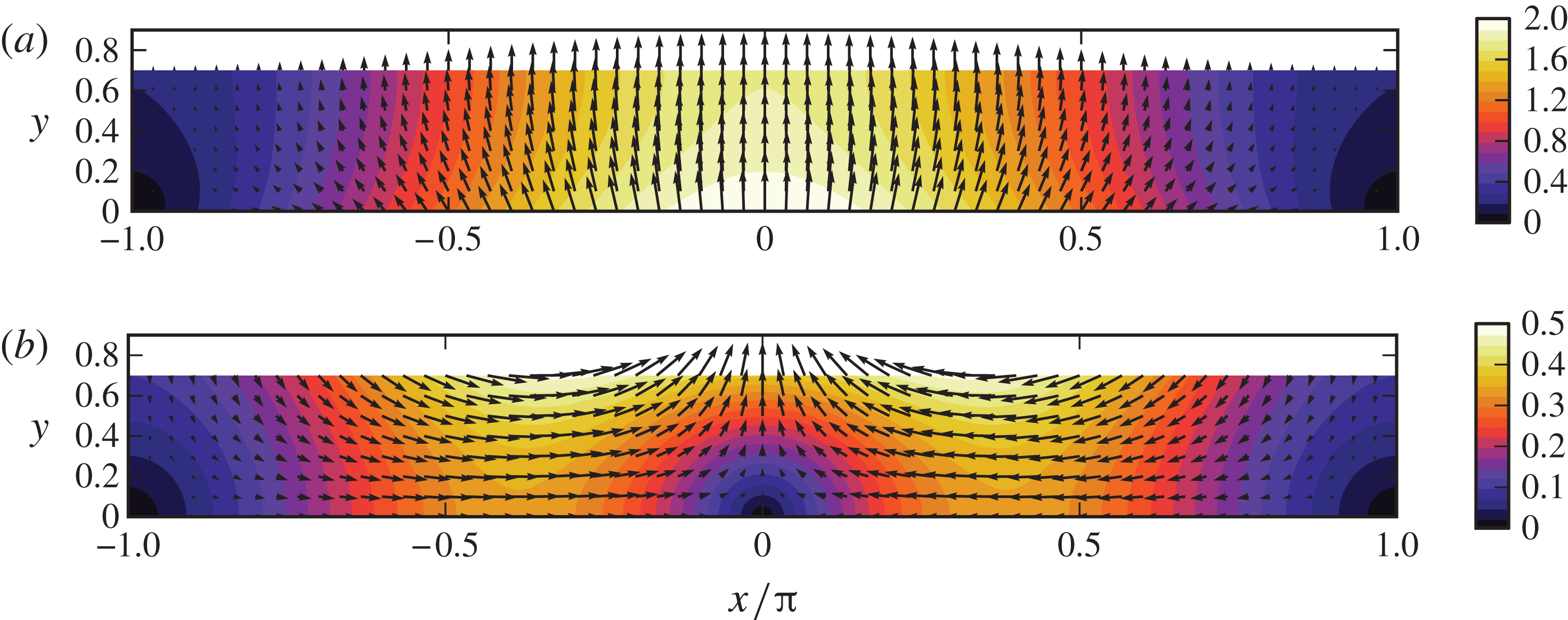
The remnant velocity field
 $\boldsymbol{u}_{2}$
is plotted in figure 3(b) for
 ${\it\beta}=0.7$
, a typical value used in experiments. For comparison, the impulsive
 $O({\it\epsilon})$
solution is plotted in figure 3(a). The horizontal component of the initial flow is directed outwards from the crest of the deformation at
 $x=0$
, as seen in the
 $O({\it\epsilon})$
solution, but it switches to an inward flow back towards the crest after the boundary deformation stops. This flow towards the crest is analogous to the radially inward flow in the axisymmetric problem that leads to jet formation (Brown et al.
Reference Brown, Brasz, Ventikos and Arnold2012).
Contour and vector plots of the leading-order perturbation solution for the velocity field at (a)
 $t\ll 1$
and (b)
 $t\gg 1$
for the case
 ${\it\beta}=0.7$
. For small
 $t$
, the
 $O({\it\epsilon})$
solution dominates, so
 $\boldsymbol{u}_{1}/f(t)$
is plotted in panel (a). The
 $O({\it\epsilon})$
solution decays proportionally to
 $f(t)$
, leaving constant terms in the
 $O({\it\epsilon}^{2})$
solution
 $\boldsymbol{u}_{2}$
for
 $t\gg 1$
, which is plotted in panel (b).

We can physically understand the dynamics of the flow as follows. The initial motion of the solid boundary primarily accelerates the fluid vertically and creates positive impulsive pressures. Because the boundary velocity varies sinusoidally with
 $x$
, the impulsive pressure is highest where the boundary velocity is highest, at the crest, and this causes an outward horizontal component of the fluid velocity. The subsequent deceleration of the boundary towards a steady-state shape produces negative pressures that eliminate all momentum at leading order, but leave a residual inward momentum at
 $O({\it\epsilon}^{2})$
. This residual inward flow arises from the nonlinearity of the free-surface motion, since no residual flow would remain if the free surface were removed, even for large
 ${\it\epsilon}$
, as the flow would depend only on instantaneous boundary conditions.
The
 $x$
dependences of the velocity components are combinations of simple sinusoids, but the
 $y$
dependences are more complicated and vary with
 ${\it\beta}$
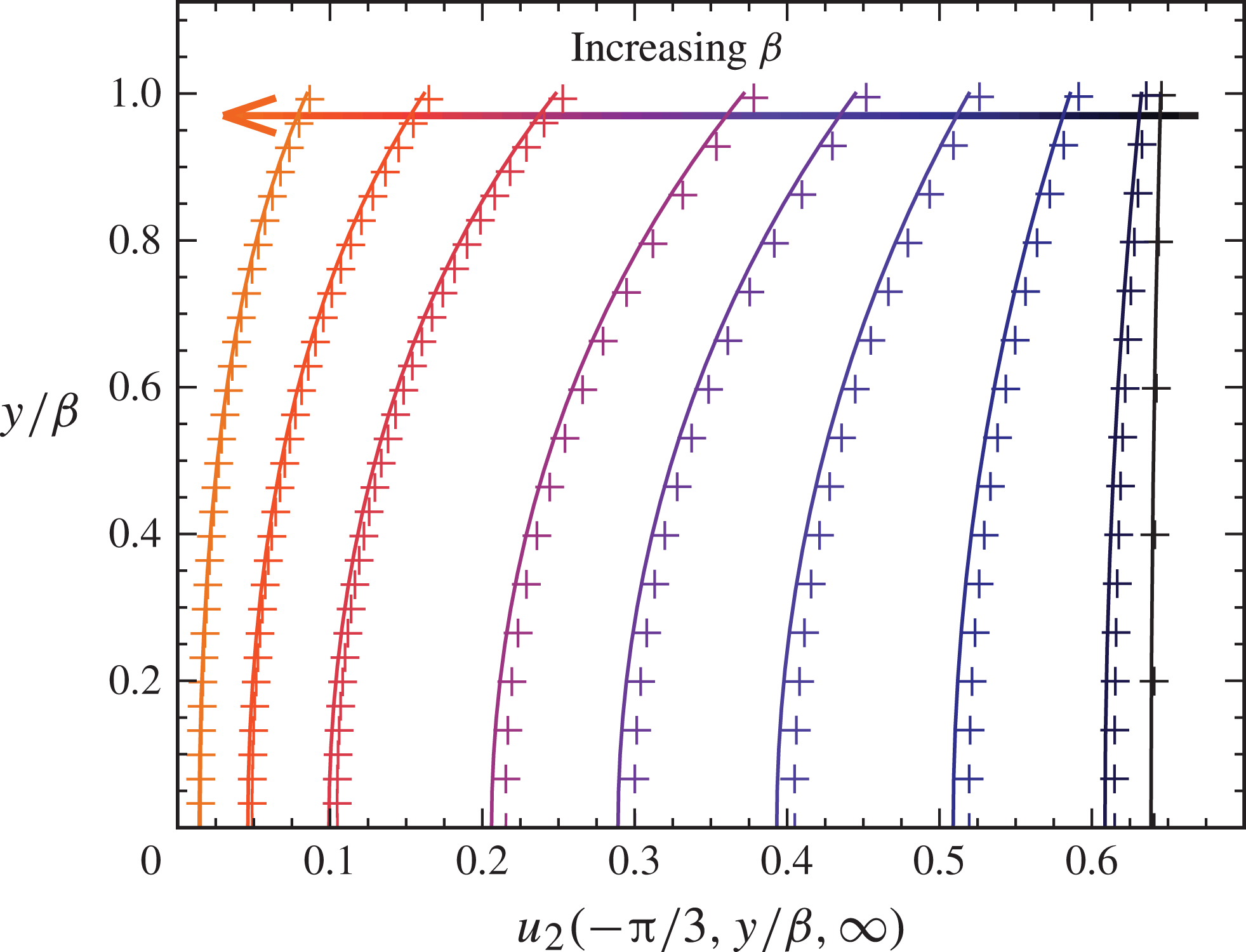
. Vertical profiles of
 $u_{2}$
at
 $x=-{\rm\pi}/3$
(where
 $u_{2}$
reaches a maximum) and
 $v_{2}$
at
 $x=0$
for
 $t\gg 1$
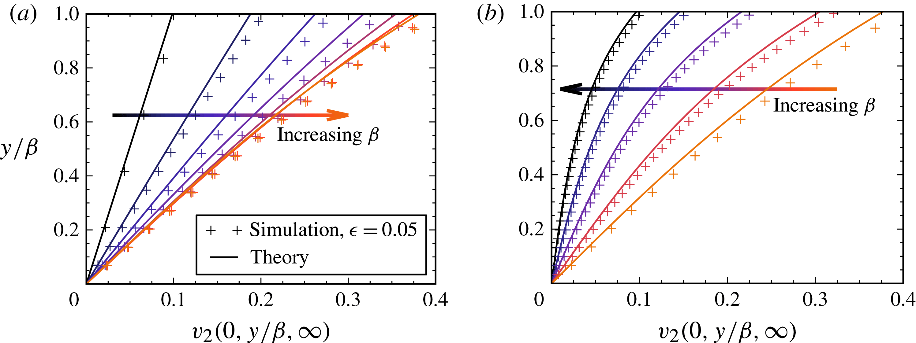
are plotted in figures 4 and 5, respectively. In the small-
 ${\it\beta}$
limit, the horizontal velocity
 $u_{2}$
approaches a uniform maximum across the layer, as expected for a shallow inviscid flow, and by mass conservation
 $v_{2}$
is linear in
 $y$
. The vertical velocity at
 $x=0$
reaches its largest value for an intermediate value of
 ${\it\beta}$
, which can be found by maximizing
 $v_{2}(0,{\it\beta},\infty )$
with respect to
 ${\it\beta}$
, yielding
 ${\it\beta}_{v}\approx 0.706$
.
Vertical profiles of the
 $O({\it\epsilon}^{2})$
remnant horizontal velocity field,
 $u_{2}$
, at
 $x=-{\rm\pi}/3$
and
 $t\gg 1$
. The values of
 ${\it\beta}$
represented in the curves are 0.1, 0.2, 0.4, 0.6, 0.8, 1.0, 1.4, 1.8 and 2.4. Corresponding results from numerical simulations, discussed in § 7, are included as
 $u/{\it\epsilon}^{2}$
at
 $t=20$
and denoted by symbols.

Vertical profiles of the
 $O({\it\epsilon}^{2})$
remnant vertical velocity field,
 $v_{2}$
, at
 $x=0$
for various values of
 ${\it\beta}$
at
 $t\gg 1$
. The critical value of
 ${\it\beta}_{v}\approx 0.706$
is used to divide the profiles for clarity, with
 ${\it\beta}$
ranging in (a) from 0.1 to 0.7 with an increment of 0.1 and in (b) from 0.8 to 2.4 with an increment of 0.4. Corresponding results from numerical simulations, discussed in § 7, are included as
 $v/{\it\epsilon}^{2}$
at
 $t=20$
.

The remnant flow deforms the free surface, and the height
 $h_{2}$
can be obtained by integrating (3.23), which leads to
 $$\begin{eqnarray}h_{2}(x,t)=\left(\cos x\,\frac{\sinh {\it\beta}}{2\cosh ^{2}{\it\beta}}+2\cos 2x\,\frac{\sinh ^{2}{\it\beta}}{\sinh 4{\it\beta}}\right)\left(t-\frac{1}{2}\text{e}^{-2t}+2\text{e}^{-t}-\frac{3}{2}\right).\end{eqnarray}$$
At long times,
 $h_{2}$
increases linearly with
 $t$
, as expected from the constant remnant velocity field. In § 7.3, we compare analytical and numerical results for the free-surface shape.
4.1. Alternative forms for
$f(t)$

Choosing alternative functional forms for
 $f(t)$
gives essentially the same results as just discussed. The time-dependent solution will naturally depend on the form of
 $f(t)$
, but the final
 $O({\it\epsilon}^{2})$
solution is found to be unchanged apart from a numerical factor in
 $\lim _{t\rightarrow \infty }a_{n}(t)$
that uniformly scales the velocity field. The spatial structure of the
 $O({\it\epsilon}^{2})$
remnant flow is therefore independent of
 $f(t)$
.
The numerical factor
 $\lim _{t\rightarrow \infty }a_{n}(t)$
can be found by rearranging (3.21) to obtain
 $$\begin{eqnarray}{\dot{a}}_{n}(t)=c_{n}\left(f^{2}(t)-2\frac{\text{d}}{\text{d}t}[\,f(t)F(t)]\right).\end{eqnarray}$$
Since
 $F(0)=0$
and
 $\lim _{t\rightarrow \infty }f(t)=0$
, integrating (4.5) results in
 $$\begin{eqnarray}\lim _{t\rightarrow \infty }a_{n}(t)=c_{n}\int _{0}^{\infty }f^{2}(t)\text{d}t.\end{eqnarray}$$
Moreover, from (3.20)
 $b_{n}(t)\sim -a_{n}(t)\tanh n{\it\beta}$
as
 $t\rightarrow \infty$
. Hence the magnitude of the entire
 $O({\it\epsilon}^{2})$
velocity field (3.22) after the boundary stops moving is directly proportional to the factor
 $\int _{0}^{\infty }f^{2}(t)\text{d}t$
.
For a fixed displacement
 $\int _{0}^{\infty }f(t)\text{d}t$
, the remnant flow is proportional to the speed of the boundary deformation, or, equivalently, inversely proportional to the time scale of the deformation. This feature can be shown by defining a boundary displacement
 $G(t)=F(t/m)$
with time rescaled by a factor
 $m$
. Then
 $g(t)={\dot{G}}(t)=f(t/m)/m$
and
 $$\begin{eqnarray}\int _{0}^{\infty }g^{2}(t)\text{d}t=\frac{1}{m}\int _{0}^{\infty }f^{2}(t)\text{d}t.\end{eqnarray}$$
Therefore, the magnitude of the remnant velocity associated with the deformation
 $G(t)$
is
 $m$
times smaller than the remnant velocity after the deformation
 $F(t)$
, while the time scale for
 $G(t)$
to approach 1 is
 $m$
times longer than for
 $F(t)$
.
5. Kinetic energy in the fluid
The kinetic energy remaining in the fluid after boundary deformation is of interest for understanding the strength of the resulting jet. It also provides a simple estimate for the energy available to eventually form a drop.
In dimensional form, the total kinetic energy in the fluid per unit width into the page is given by the integral
 $$\begin{eqnarray}\bar{E}_{k}(t)=\frac{{\it\rho}}{2k^{4}{\it\tau}^{2}}\int _{-{\rm\pi}}^{{\rm\pi}}\int _{h_{b}(x,t)}^{h(x,t;{\it\epsilon})}(u^{2}+v^{2})\text{d}y\text{d}x.\end{eqnarray}$$
The integral in
 $y$
is replaced by the domain perturbation
 $$\begin{eqnarray}\displaystyle \int _{h_{b}}^{h}\!f(y)\text{d}y & = & \displaystyle \int _{0}^{{\it\beta}}\!f(y)\text{d}y+(h-{\it\beta})\,f({\it\beta})-h_{b}\,f(0)\nonumber\\ \displaystyle & & \displaystyle \hspace{45.60004pt}+\,\frac{1}{2}(h-{\it\beta})^{2}\left.\frac{\text{d}f}{\text{d}y}\right|_{y={\it\beta}}-\frac{1}{2}h_{b}^{2}\left.\frac{\text{d}f}{\text{d}y}\right|_{y=0}+\cdots \,.\end{eqnarray}$$
Upon non-dimensionalization of the kinetic energy by
 ${\it\rho}/(k^{4}{\it\tau}^{2})$
and substitution of the expansion (3.2) for the velocity field, we obtain
 $$\begin{eqnarray}E_{k}(t)=\frac{{\it\epsilon}^{2}}{2}\int _{-{\rm\pi}}^{{\rm\pi}}\left[\int _{0}^{{\it\beta}}I\text{d}y+\mathop{\sum }_{j=0}^{\infty }\left(\frac{(h-{\it\beta})^{j+1}}{(\,j+1)!}\left.\frac{\partial ^{j}I}{\partial y^{j}}\right|_{y={\it\beta}}-\frac{h_{b}^{j+1}}{(\,j+1)!}\left.\frac{\partial ^{i}I}{\partial y^{i}}\right|_{y=0}\right)\right]\!\text{d}x,\end{eqnarray}$$
where
 $I(x,y,t)=\sum _{j=0}^{\infty }{\it\epsilon}^{i}I_{i}$
and
 $$\begin{eqnarray}\displaystyle I_{0}(x,y,t) & = & \displaystyle u_{1}^{2}+v_{1}^{2},\end{eqnarray}$$
 $$\begin{eqnarray}\displaystyle I_{1}(x,y,t) & = & \displaystyle 2(u_{1}u_{2}+v_{1}v_{2}),\end{eqnarray}$$
 $$\begin{eqnarray}\displaystyle I_{2}(x,y,t) & = & \displaystyle u_{2}^{2}+v_{2}^{2}+2(u_{1}u_{3}+v_{1}v_{3}).\end{eqnarray}$$
We include terms up to
 $O({\it\epsilon}^{4})$
because
 $u_{1}$
and
 $v_{1}$
decrease exponentially with time, so the
 $O({\it\epsilon}^{2})$
and
 $O({\it\epsilon}^{3})$
terms will not contribute to the kinetic energy remaining after the boundary motion stops. This behaviour also means that we can safely neglect the products
 $u_{1}u_{3}$
and
 $v_{1}v_{3}$
when considering the final kinetic energy.
For the full time evolution of the kinetic energy, we divide it as
 $E_{k}(t)=E_{k,2}(t)+E_{k,3}(t)+E_{k,4}(t)+\cdots \,$
, where
 $E_{k,n}(t)$
contains the
 $O({\it\epsilon}^{n})$
contributions. At early times,
 $E_{k,2}(t)$
will dominate. Eventually,
 $E_{k,2}(t)$
and
 $E_{k,3}(t)$
will approach 0, but
 $E_{k,4}(t)$
will remain non-zero, approaching a fixed value for
 $t\gg 1$
.
We start with the kinetic energy at early times, which is given by
 $$\begin{eqnarray}E_{k,2}(t)=\frac{{\it\epsilon}^{2}}{2}\int _{0}^{{\it\beta}}\!\int _{-{\rm\pi}}^{{\rm\pi}}(u_{1}^{2}+v_{1}^{2})\text{d}x\text{d}y.\end{eqnarray}$$
Substituting
 $u_{1}$
and
 $v_{1}$
from (3.13) and integrating results in
 $$\begin{eqnarray}E_{k,2}(t)={\rm\pi}{\it\epsilon}^{2}({\textstyle \frac{1}{2}}\tanh {\it\beta}+{\it\beta})f^{2}(t).\end{eqnarray}$$
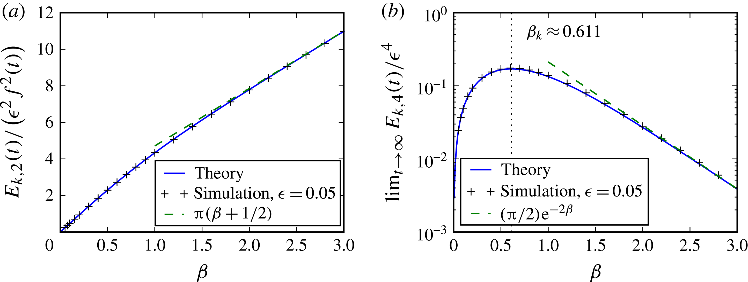
The
 ${\it\beta}$
dependence is plotted in figure 6(a), which shows that the kinetic energy increases approximately linearly with
 ${\it\beta}$
. This feature comes from the 1 in the
 $1+\cos x$
form for
 $V_{b}(x,t)$
, which induces a constant velocity flow everywhere in the fluid, together with the fact that the volume of the film increases linearly with
 ${\it\beta}$
.
The
 ${\it\beta}$
dependence of the kinetic energy in the fluid layer due to the (a)
 $O({\it\epsilon})$
and (b)
 $O({\it\epsilon}^{2})$
velocity fields. At early times, the
 $O({\it\epsilon})$
solution dominates, but, as the boundary motion slows and
 $f(t)$
approaches zero, the
 $O({\it\epsilon}^{2})$
velocity field remains non-zero, leaving kinetic energy in the fluid. Corresponding results from numerical simulations, discussed in § 7, are included at times (a)
 $t=0$
and (b)
 $t=20$
.

At early times,
 $E_{k,3}(t)$
and
 $E_{k,4}(t)$
will also contribute, although the extra factors of
 ${\it\epsilon}$
and the fact that
 $u_{2}=v_{2}=h_{1}=F(t)=0$
at
 $t=0$
make them only a minor correction to
 $E_{k,2}(t)$
. For example,
 $E_{k,3}(t)$
is given by the integral
 $$\begin{eqnarray}\displaystyle E_{k,3}(t) & = & \displaystyle \frac{{\it\epsilon}^{3}}{2}\int _{-{\rm\pi}}^{{\rm\pi}}\bigg(\int _{0}^{{\it\beta}}2(u_{1}u_{2}+v_{1}v_{2})\text{d}y+h_{1}(u_{1}^{2}+v_{1}^{2})_{y={\it\beta}}\nonumber\\ \displaystyle & & \displaystyle \hspace{44.39996pt}-\,(1+\cos x)F(t)(u_{1}^{2}+v_{1}^{2})_{y=0}\bigg)\text{d}x,\end{eqnarray}$$
which simplifies to
 $$\begin{eqnarray}E_{k,3}(t)=-{\rm\pi}{\it\epsilon}^{3}F(t)\,f^{2}(t)\tanh ^{2}{\it\beta},\end{eqnarray}$$
where (3.20) has been used to eliminate
 $a_{1}(t)\tanh {\it\beta}+b_{1}(t)$
.
5.1. Kinetic energy remaining when
$t\gg 1$

After the boundary motion stops, the remaining kinetic energy can be computed by integrating the non-zero
 $O({\it\epsilon}^{2})$
solution for the velocity field. We start with
 $$\begin{eqnarray}E_{k,4}(t)=\frac{{\it\epsilon}^{4}}{2}\int _{0}^{{\it\beta}}\!\int _{-{\rm\pi}}^{{\rm\pi}}(u_{2}^{2}+v_{2}^{2}+2u_{1}u_{3}+2v_{1}v_{3})\text{d}x\text{d}y+\text{boundary terms},\end{eqnarray}$$
where the boundary terms include integrals of
 $h_{1}\,\partial I_{0}/\partial y$
,
 $h_{1}I_{1}$
,
 $h_{1}^{2}I_{0}$
,
 $h_{2}I_{0}$
and corresponding terms for
 $h_{b}$
. We take the limit
 $t\rightarrow \infty$
to eliminate
 $u_{1}u_{3}$
,
 $v_{1}v_{3}$
and the boundary terms, as they all contain at least one factor proportional to
 $f(t)$
. Substitution of the solution given in (3.22a
) and (3.22b
) then leads to
 $$\begin{eqnarray}\displaystyle \lim _{t\rightarrow \infty }E_{k,4}(t) & = & \displaystyle \lim _{t\rightarrow \infty }\frac{{\rm\pi}{\it\epsilon}^{4}}{4}\left\{[a_{1}^{2}(t)+b_{1}^{2}(t)]\sinh 2{\it\beta}+2[a_{2}^{2}(t)+b_{2}^{2}(t)]\sinh 4{\it\beta}\right.\nonumber\\ \displaystyle & & \displaystyle \hspace{48.0pt}\left.+\,4(a_{1}b_{1}\sinh ^{2}{\it\beta}+2a_{2}b_{2}\sinh ^{2}2{\it\beta})\right\}.\end{eqnarray}$$
We can substitute (4.6) and (3.20) for, respectively,
 $a_{n}(t)$
and
 $b_{n}(t)$
to show that the remaining kinetic energy after boundary deformation is
 $$\begin{eqnarray}\lim _{t\rightarrow \infty }E_{k,4}(t)=\frac{{\rm\pi}{\it\epsilon}^{4}}{8}\left(\frac{2\sinh 3{\it\beta}-\sinh {\it\beta}}{\cosh ^{3}{\it\beta}\,\cosh 2{\it\beta}}\right)\left(\int _{0}^{\infty }f^{2}(t)\text{d}t\right)^{2}.\end{eqnarray}$$
The
 ${\it\beta}$
dependence of
 $E_{k,4}$
in (5.11) is plotted in figure 6(b) for
 $f(t)=\text{e}^{-t}$
. The remnant kinetic energy diminishes rapidly with
 ${\it\beta}$
for
 ${\it\beta}>1$
, especially given that the initial kinetic energy increases with
 ${\it\beta}$
; for large
 ${\it\beta}$
,
 $\lim _{t\rightarrow \infty }E_{k,4}(t)\sim ({\rm\pi}/2){\it\epsilon}^{4}\text{e}^{-2{\it\beta}}$
while
 $E_{k,2}(t)\sim {\rm\pi}{\it\epsilon}^{2}({\it\beta}+1/2)\,f^{2}(t)$
.
The maximum in
 $\lim _{t\rightarrow \infty }E_{k,4}(t)$
with respect to
 ${\it\beta}$
is found at
 ${\it\beta}_{k}\approx 0.611$
. This value is similar to the value
 ${\it\beta}_{v}\approx 0.706$
found earlier, which maximizes
 $v_{2}$
at
 $x={\rm\pi}/2$
and
 $y={\it\beta}$
. These maximizing values of
 ${\it\beta}$
suggest an optimal region for jet formation. In particular,
 ${\it\beta}_{k}$
maximizes the energy transfer from the deforming solid to the liquid layer. Note that, because the remnant flow is proportional to
 $\int _{0}^{\infty }f^{2}(t)\text{d}t$
, the maximizing values of
 ${\it\beta}$
are independent of the form of
 $f(t)$
.
5.2. Transition from the
$O({\it\epsilon})$
to the
$O({\it\epsilon}^{2})$
regime


With
 $E_{k,2}(t)$
and
 $\lim _{t\rightarrow \infty }E_{k,4}(t)$
defined by (5.6) and (5.10), respectively, we have a leading-order time evolution for the kinetic energy. One quantity of interest here is the transition time
 $t^{\ast }$
when the energy in the
 $O({\it\epsilon})$
solution decays below that of the
 $O({\it\epsilon}^{2})$
solution that remains at
 $t\gg 1$
. Analytically,
 $t^{\ast }$
can be found by equating
 $E_{k,2}(t^{\ast })$
with
 $\lim _{t\rightarrow \infty }E_{k,4}(t)$
, yielding
 $$\begin{eqnarray}t^{\ast }=\log \frac{1}{{\it\epsilon}}-\frac{1}{2}\log \left(\frac{2\sinh 3{\it\beta}-\sinh {\it\beta}}{16\cosh ^{3}{\it\beta}\cosh 2{\it\beta}\,(2{\it\beta}+\tanh {\it\beta})}\right)\end{eqnarray}$$
for
 $f(t)=\text{e}^{-t}$
.
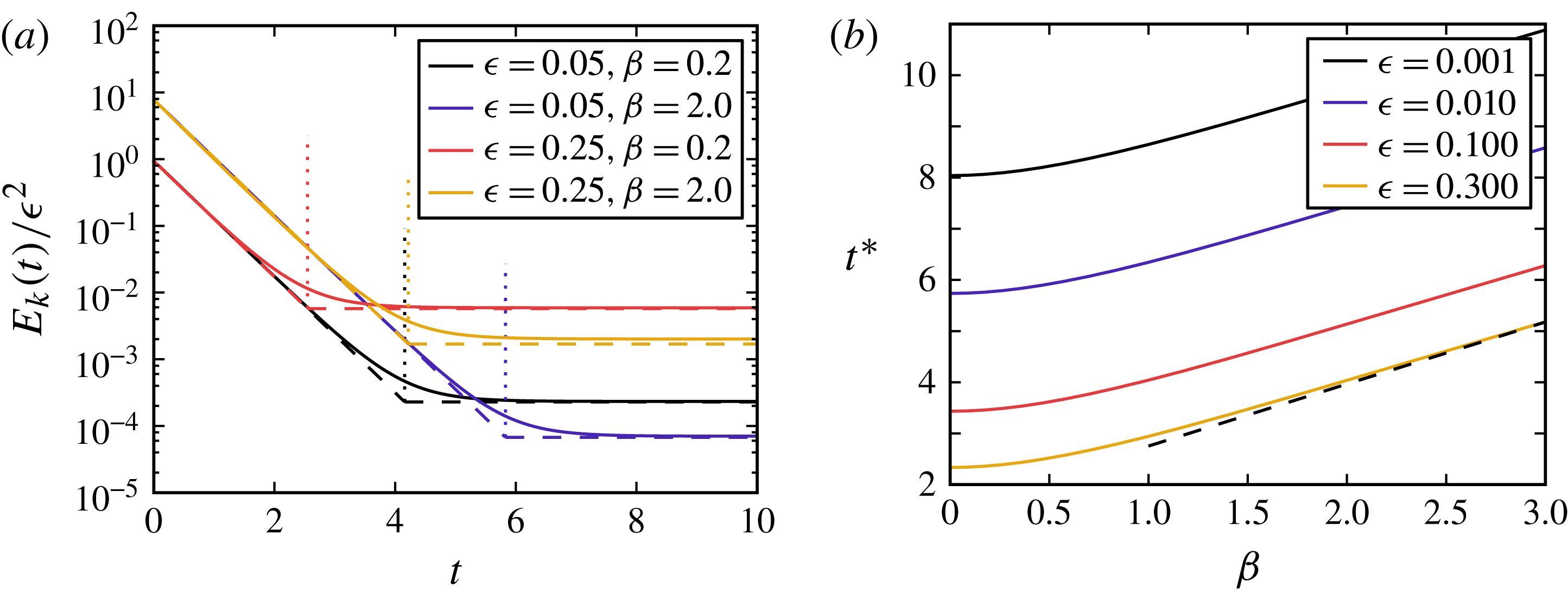
We can determine the time evolution of the energy for various values of
 ${\it\epsilon}$
and
 ${\it\beta}$
and the dependence of transition times on
 ${\it\beta}$
; these results are shown in figure 7. Initially, the kinetic energy in the fluid decreases exponentially with time, in accord with the exponentially decreasing boundary velocity and the associated
 $O({\it\epsilon})$
velocity field. At the transition time
 $t^{\ast }$
, this energy decays below the constant kinetic energy of the
 $O({\it\epsilon}^{2})$
velocity field. We see that, as
 ${\it\epsilon}$
decreases or
 ${\it\beta}$
increases, it takes longer for the
 $O({\it\epsilon}^{2})$
solution to overtake the
 $O({\it\epsilon})$
solution; the transition time is roughly inversely correlated with the final energy of the flow.
(a) The time evolution of the kinetic energy in the fluid for four sets of parameters, normalized by
 ${\it\epsilon}^{2}$
so that
 $O({\it\epsilon})$
solutions collapse for a given
 ${\it\beta}$
. Solid curves denote results from numerical simulations, discussed in § 7, while dashed lines denote the leading-order behaviour,
 $E_{k,2}(t)$
for
 $t<t^{\ast }$
and
 $\lim _{t\rightarrow \infty }E_{k,4}(t)$
for
 $t>t^{\ast }$
. The transition time
 $t^{\ast }$
, given by (5.12), is included as a vertical dotted line for each curve. (b) The
 ${\it\beta}$
dependence of
 $t^{\ast }$
for select values of
 ${\it\epsilon}$
, along with the asymptote
 $t^{\ast }\sim \log (1/{\it\epsilon})+{\it\beta}+(\log (2{\it\beta}+1))/2$
for large
 ${\it\beta}$
.

6. Extension to an axisymmetric domain
The practical application to jet formation arises from an axisymmetric boundary deformation, so the extension of the domain-perturbation calculation from two dimensions to an axisymmetric domain is discussed here.
For illustration, the radial dependence of the boundary deformation is assumed to be a Gaussian, taking the form
 $$\begin{eqnarray}\bar{h}_{b}(\bar{r},\bar{t})=\text{e}^{-\bar{r}^{2}/(2c^{2})}\bar{F}(\bar{t}).\end{eqnarray}$$
This functional form is similar to the one used in Brown et al. (Reference Brown, Brasz, Ventikos and Arnold2012), as discussed in § 8, while keeping the domain-perturbation calculation from being too complicated.
Non-dimensionalizing lengths by
 $c$
now leads to
 $$\begin{eqnarray}h_{b}(r,t)={\it\epsilon}\text{e}^{-r^{2}/2}F(t),\end{eqnarray}$$
with dimensionless parameters
 ${\it\beta}\equiv H/c$
and
 ${\it\epsilon}\equiv H_{b}/c$
.
With axisymmetric forcing, the Fourier sum of sines and cosines from the two-dimensional (2D) calculation is replaced by a Hankel transform with Bessel functions of the first kind of order zero,
 $J_{0}(kr)$
. The solution to
 ${\rm\nabla}^{2}{\it\phi}=0$
in a layer of height
 ${\it\beta}$
can be written as
 $$\begin{eqnarray}{\it\phi}(r,z,t)=\int _{0}^{\infty }(A(k,t)\cosh [k({\it\beta}-z)]+B(k,t)\sinh [k({\it\beta}-z)])J_{0}(kr)\text{d}k+C(t)z,\end{eqnarray}$$
where
 $A(k,t)$
,
 $B(k,t)$
and
 $C(t)$
are time-dependent functions that must be determined.
Details of the axisymmetric domain-perturbation solution are provided in appendix A, and the main results are quoted here. The velocity potentials at
 $O({\it\epsilon})$
for all
 $t$
, and at
 $O({\it\epsilon}^{2})$
for
 $t\gg 1$
, are given as
 $$\begin{eqnarray}{\it\phi}_{1}(r,z,t)=-f(t)\int _{0}^{\infty }\text{e}^{-k^{2}/2}\frac{\sinh [k({\it\beta}-z)]}{\cosh {\it\beta}k}J_{0}(kr)\text{d}k\equiv f(t){\it\Phi}_{1}(r,z),\end{eqnarray}$$
 $$\begin{eqnarray}{\it\phi}_{2}(r,z,\infty )=a_{\infty }\int _{0}^{\infty }\hat{A}_{2}(k)\{\cosh [k({\it\beta}-z)]-\tanh {\it\beta}k\sinh [k({\it\beta}-z)]\}J_{0}(kr)\text{d}k,\end{eqnarray}$$
respectively, where
 $$\begin{eqnarray}a_{\infty }=\frac{1}{2}\int _{0}^{\infty }f^{2}(t)\text{d}t\end{eqnarray}$$
and
 $$\begin{eqnarray}\hat{A}_{2}(k)=k\int _{0}^{\infty }\left(\left.\frac{\partial {\it\Phi}_{1}}{\partial z}\right|_{z={\it\beta}}\right)^{2}J_{0}(kr)r\text{d}r.\end{eqnarray}$$
Many features of the solution are unchanged from the 2D case; the
 $O({\it\epsilon})$
velocity field is still proportional to
 $f(t)$
, and the
 $O({\it\epsilon}^{2})$
remnant velocity field is still proportional to
 $\int _{0}^{\infty }f^{2}(t)\text{d}t$
. The spatial dependence of the remnant velocity field is completely independent of the time dependence of the boundary deformation,
 $f(t)$
.
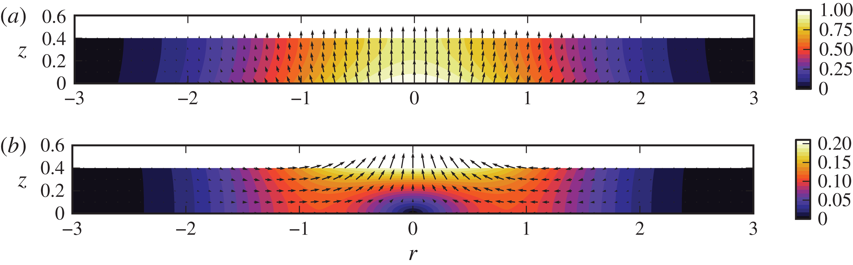
Contour and vector plots of the leading-order perturbation solution for the axisymmetric velocity field for (a)
 $t\ll 1$
and (b)
 $t\gg 1$
for the case
 ${\it\beta}=0.4$
. For small
 $t$
, the
 $O({\it\epsilon})$
solution dominates, so
 $\boldsymbol{u}_{1}/f(t)$
is plotted in panel (a). The
 $O({\it\epsilon})$
solution decays proportionally to
 $f(t)$
, leaving constant terms in the
 $O({\it\epsilon}^{2})$
solution
 $\boldsymbol{u}_{2}$
for
 $t\gg 1$
, which is plotted in panel (b).

The integrals in
 ${\it\phi}_{1}(r,z,t)$
,
 ${\it\phi}_{2}(r,z,t)$
and
 $\hat{A}_{2}(k)$
do not appear to have closed-form expressions, so to examine the velocity field or kinetic energy they must be integrated numerically for each value of
 ${\it\beta}$
. Taking
 $f(t)=\text{e}^{-t}$
again, the remnant velocity field is computed and plotted in figure 8 for
 ${\it\beta}=0.4$
, which is close to the critical value
 ${\it\beta}_{v}\approx 0.384$
that maximizes
 $v_{2}(0,{\it\beta},\infty )$
. (As discussed in § 9, the difference from the 2D value
 ${\it\beta}_{v}\approx 0.706$
is largely due to the different definitions of
 ${\it\beta}$
for sinusoidal and Gaussian wave forms.) Qualitatively, the main difference between the axisymmetric and 2D remnant velocity fields is the radial focusing of the axisymmetric case, in which the velocities are largest near
 $(r,z)=(0,{\it\beta})$
and decay more rapidly with increasing
 $r$
. This behaviour contrasts with the less focused 2D velocity field of figure 3(b), in which the largest velocities are mostly horizontal and near
 $x=\pm 0.33{\rm\pi}$
. The relative uniformity of the 2D flow field is partly due to the periodic nature of the boundary deformation, but 2D simulations of the flow induced by a Gaussian boundary deformation exhibit the same behaviour as simulations with the sinusoidal deformation; inward horizontal velocities at some
 $x>0$
are still larger than the vertical velocities at
 $x=0$
, which differs from the axisymmetric results.
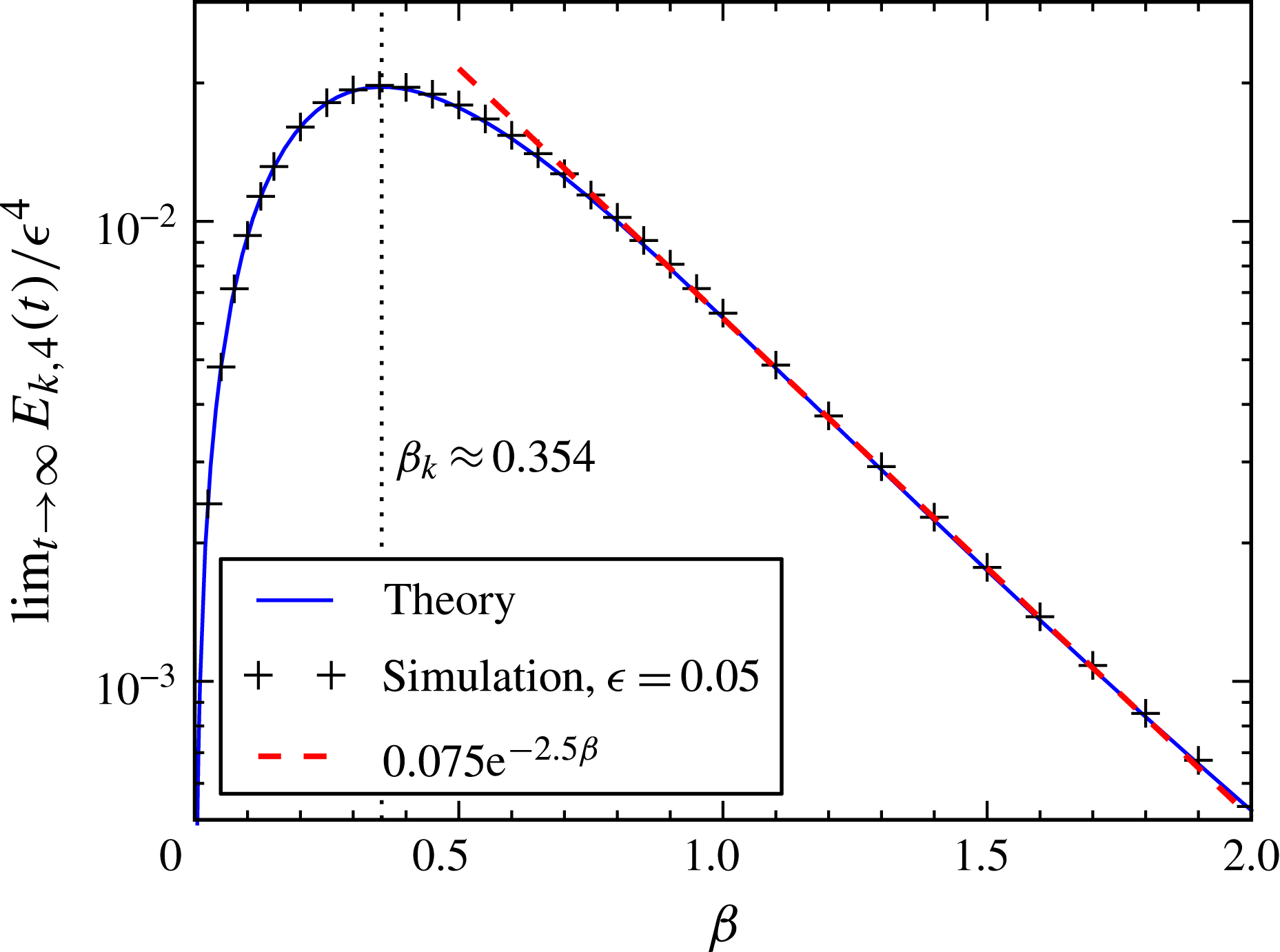
The remnant kinetic energy is computed by numerical integration of the velocity field and plotted in figure 9. The shape of the curve is similar to the 2D case, with differences appearing in the value of
 ${\it\beta}$
maximizing kinetic energy (
 ${\it\beta}_{k}\approx 0.354$
instead of
 ${\it\beta}_{k}\approx 0.611$
as in the 2D case) and the asymptotic behaviour at large
 ${\it\beta}$
; the remnant kinetic energy in the axisymmetric case decays proportionally to
 $\text{e}^{-2.5{\it\beta}}$
, as opposed to
 $\text{e}^{-2{\it\beta}}$
in the 2D case.
The
 ${\it\beta}$
dependence of the remnant kinetic energy in the fluid layer due to the
 $O({\it\epsilon}^{2})$
axisymmetric velocity field. Corresponding results from numerical simulations are included at
 $t=20$
along with an exponential fit for large
 ${\it\beta}$
.

The transition time at which the kinetic energy from the remnant
 $O({\it\epsilon}^{2})$
velocity field overtakes the decaying
 $O({\it\epsilon})$
solution is straightforward to deduce given the kinetic energies. We first write
 $$\begin{eqnarray}E_{k,2}(t)={\it\epsilon}^{2}\hat{E}_{k,2}({\it\beta})\,f^{2}(t),\quad \lim _{t\rightarrow \infty }E_{k,4}(t)={\it\epsilon}^{4}\hat{E}_{k,4}({\it\beta}).\end{eqnarray}$$
For
 $f(t)=\text{e}^{-t}$
, we can then find the time
 $t^{\ast }$
at which
 $E_{k,2}(t)=\lim _{t\rightarrow \infty }E_{k,4}(t)$
with
 $$\begin{eqnarray}t^{\ast }=\log \left(\frac{1}{{\it\epsilon}}\right)+\frac{1}{2}\log \left(\frac{\hat{E}_{k,2}({\it\beta})}{\hat{E}_{k,4}({\it\beta})}\right).\end{eqnarray}$$
Note that
 $\hat{E}_{k,2}({\it\beta})$
and
 $\hat{E}_{k,4}({\it\beta})$
depend only on
 ${\it\beta}$
, so the
 ${\it\epsilon}$
and
 ${\it\beta}$
dependences are separate in (6.5), as in (5.12).
While the quantitative details of the axisymmetric solution differ from the 2D solution, partly due to the choice of shape function
 $h_{b}$
, the physical flow observed and the structure of the solution in the axisymmetric case are qualitatively unchanged relative to the 2D case.
7. Numerical simulations
The domain-perturbation solution is asymptotically correct in the limit
 ${\it\epsilon}\rightarrow 0$
, but a finite
 ${\it\epsilon}>0$
is required to generate an impulse strong enough to form a liquid jet. We therefore solved Laplace’s equation numerically to confirm the above analytical results and test their range of validity.
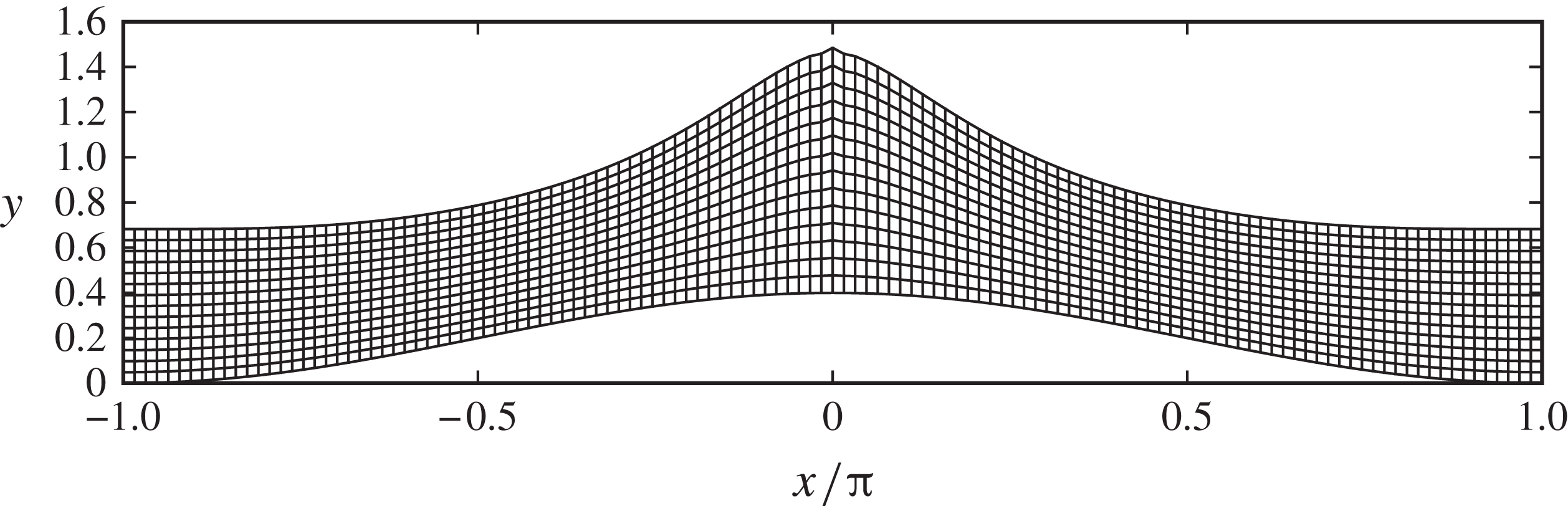
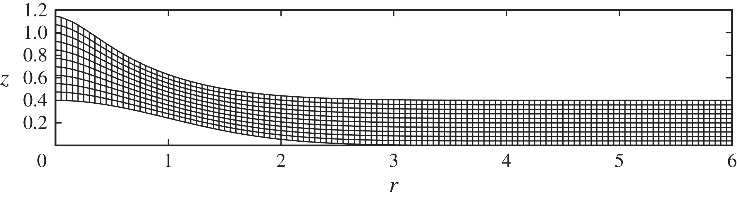
Laplace’s equation is solved using central finite differences in curvilinear coordinates on a moving mesh, which allows both the solid boundary and the free surface to move each time step. Both 2D and axisymmetric domains can be simulated, and details of the solution scheme are provided in appendix B.
7.1. Validation of the theory
We test the 2D theoretical results numerically by performing simulations with
 ${\it\epsilon}=0.05$
and
 $0.05\leqslant {\it\beta}\leqslant 3$
. Simulations are run from
 $t=0$
to
 $t=20$
, at which point the
 $O({\it\epsilon})$
terms are negligibly small and only
 $O({\it\epsilon}^{2})$
terms remain. Figures 4–6 compare simulation results at
 $t=20$
with the analytical
 $O({\it\epsilon}^{2})$
solution, showing excellent agreement in the
 ${\it\beta}$
dependence of vertical profiles of the velocity field and the total kinetic energy. As discussed in § 4, the remnant horizontal velocity
 $u_{2}$
, which is inwards towards the crest, decreases with increasing
 ${\it\beta}$
, and the remnant vertical velocity
 $v_{2}$
in the direction of the boundary deformation at the crest has a maximum at
 ${\it\beta}_{v}\approx 0.706$
, which is close to the value
 ${\it\beta}_{k}\approx 0.611$
that maximizes the remnant kinetic energy in the fluid.
Comparisons of velocity slices from domain-perturbation results and finite-difference simulations were also made in an axisymmetric domain for the Gaussian boundary deformation. The axisymmetric domain-perturbation results showed similarly good agreement with simulations at
 ${\it\epsilon}=0.05$
and
 $t=20$
across all values of
 ${\it\beta}$
; for brevity, these are not included here. The total kinetic energy in the axisymmetric simulations at
 $t=20$
and
 ${\it\epsilon}=0.05$
is plotted in figure 9 for varying
 ${\it\beta}$
and agrees very well with the remnant kinetic energy from the domain-perturbation results.
7.2. Dependence on
${\it\epsilon}$

The range of validity of the perturbation theory is tested by comparing simulation results for varying values of
 ${\it\epsilon}$
at fixed
 ${\it\beta}$
. While we could examine both the 2D and axisymmetric domain-perturbation solutions, for the rest of the paper we limit ourselves to the axisymmetric solutions, as they are ultimately closer to the physical jet formation scenario with which we compare in § 8. We emphasize that the qualitative features are nevertheless captured by the 2D geometry.
We focus on the value
 ${\it\beta}=0.4$
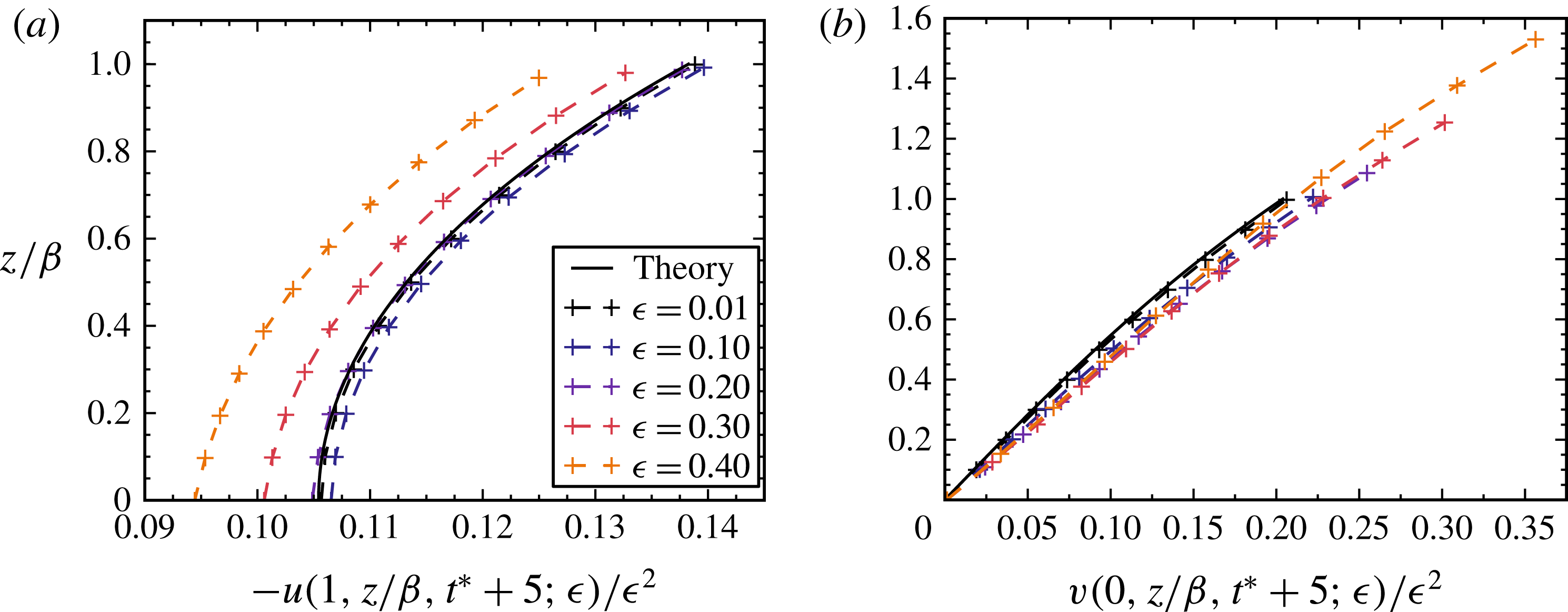
, as this is near the optimum values found earlier in our analysis for maximizing the remnant vertical jet velocity and kinetic energy in the axisymmetric case. Vertical velocity profiles for a range of
 ${\it\epsilon}$
are plotted in figure 10. Each profile is plotted at
 $t=t^{\ast }+5$
, which is long enough after the transition time
 $t^{\ast }$
that the
 $O({\it\epsilon})$
component of the solution is negligible. We see that the general shapes of the curves are similar up through
 ${\it\epsilon}=0.4$
. The plot of
 $v(0,z/{\it\beta},t^{\ast }+5;{\it\epsilon})$
shows that, as
 ${\it\epsilon}$
is increased, the simulations reach higher velocities at the free surface and the
 $z/{\it\beta}$
values are stretched to larger values due to the jet-forming deformation of the free surface at
 $r=0$
. At longer times, the velocity fields of the higher-
 ${\it\epsilon}$
cases continue to evolve as the liquid layer deforms, while the velocity fields of the lower-
 ${\it\epsilon}$
cases remain nearly constant in the
 $O({\it\epsilon}^{2})$
solution.
Comparisons between numerical simulations at
 $t=t^{\ast }+5$
and theory at
 $t\gg 1$
for slices of (a)
 $-u$
at
 $r=1$
and (b)
 $v$
at
 $r=0$
for
 ${\it\beta}=0.4$
and various values of
 ${\it\epsilon}$
. Here
 $t^{\ast }$
is the transition time defined by (6.5), which takes the approximate values 6.3, 4.0, 3.3, 2.9 and 2.6 for
 ${\it\epsilon}=0.01$
, 0.1, 0.2, 0.3 and 0.4, respectively. The
 $z$
values of grid points from the simulations are shifted down by
 $h_{b}(r)$
to account for the non-zero boundary displacement.

7.3. Free-surface evolution
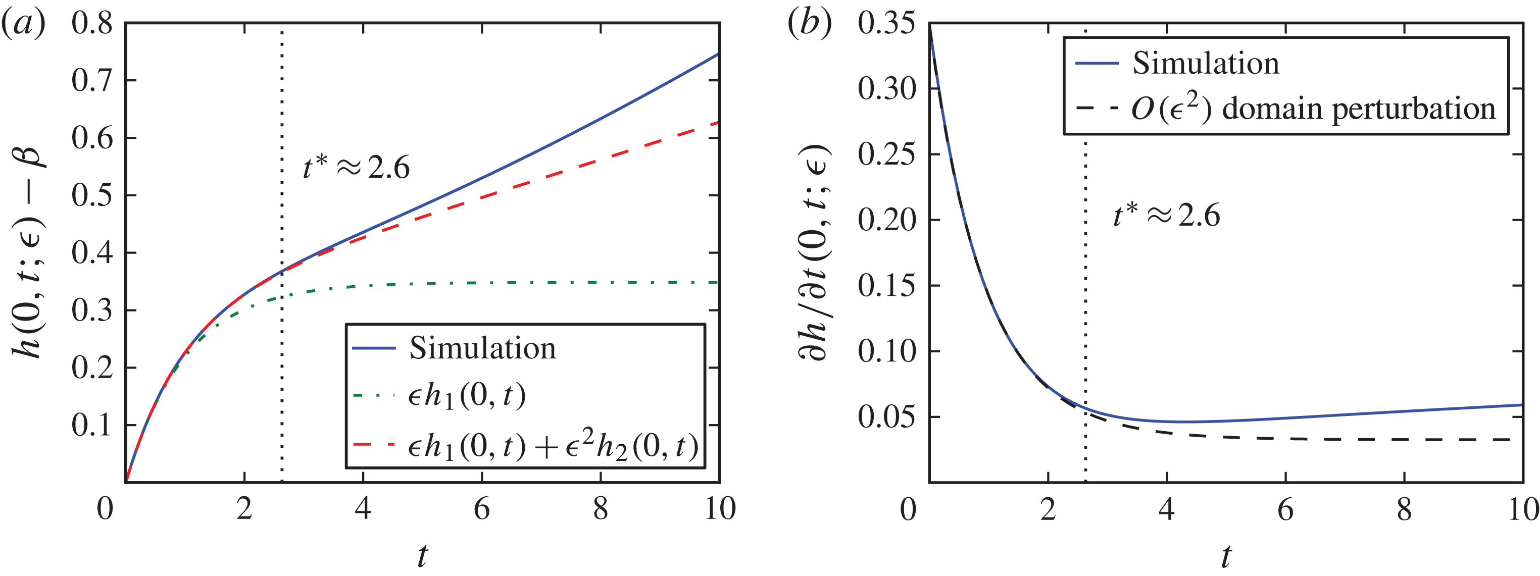
We explore the time evolution of the free surface for the test case
 ${\it\epsilon}={\it\beta}=0.4$
by investigating the ‘jet-front’ displacement, i.e.
 $h(0,t;{\it\epsilon})-{\it\beta}$
. This quantity tracks the length of the initial jet over time, and is plotted in figure 11(a). This plot illustrates the overall dynamics of the free-surface evolution; the free surface deforms rapidly in the initial stages while the solid boundary is deforming, and, as the deformation of the solid slows, the free-surface deformation slows as well until only the smaller velocity of the
 $O({\it\epsilon}^{2})$
solution remains (see also supplementary movie 1 available at http://dx.doi.org/10.1017/jfm.2015.74, which contains the time evolution of the velocity field and liquid layer deformation). Recalling the transition time (6.5) between kinetic energy associated with the
 $O({\it\epsilon})$
and
 $O({\it\epsilon}^{2})$
velocity fields, we calculate
 $t^{\ast }\approx 2.6$
for
 ${\it\epsilon}=0.4$
and
 ${\it\beta}=0.4$
. This time is indicated in figure 11(a), dividing regions of jet-front displacement into times when either the
 $O({\it\epsilon})$
or
 $O({\it\epsilon}^{2})$
velocity field dominates. According to the
 $O({\it\epsilon}^{2})$
domain-perturbation results, the jet that forms at
 $r=0$
grows in length at a constant rate as liquid flows towards the centre to feed the jet. By
 $t=10$
, the simulated jet length has started to diverge from the
 $O({\it\epsilon}^{2})$
domain-perturbation value, with the jet growth speeding up. This reflects the fact that by this stage the free-surface deformation is approaching values comparable to the initial layer depth.
Comparison of (a) jet front displacements and (b) jet velocities between axisymmetric simulation and domain-perturbation results for
 ${\it\beta}=0.4$
and
 ${\it\epsilon}=0.4$
. As the boundary deformation exponentially stops, the domain-perturbation result approaches a constant velocity while the numerically simulated velocity starts to increase.

Figure 11(b) shows that the speed of the jet increases approximately linearly with time after the boundary deformation stops. For smaller values of
 ${\it\epsilon}$
, the jet’s acceleration is smaller, and by fitting the slopes of plots of the jet velocity, we find that the acceleration
 $a\sim {\it\epsilon}^{4}$
. This result is consistent with the fact that the domain perturbation has only been carried out to
 $O({\it\epsilon}^{2})$
in velocity, so the higher-order acceleration is absent.
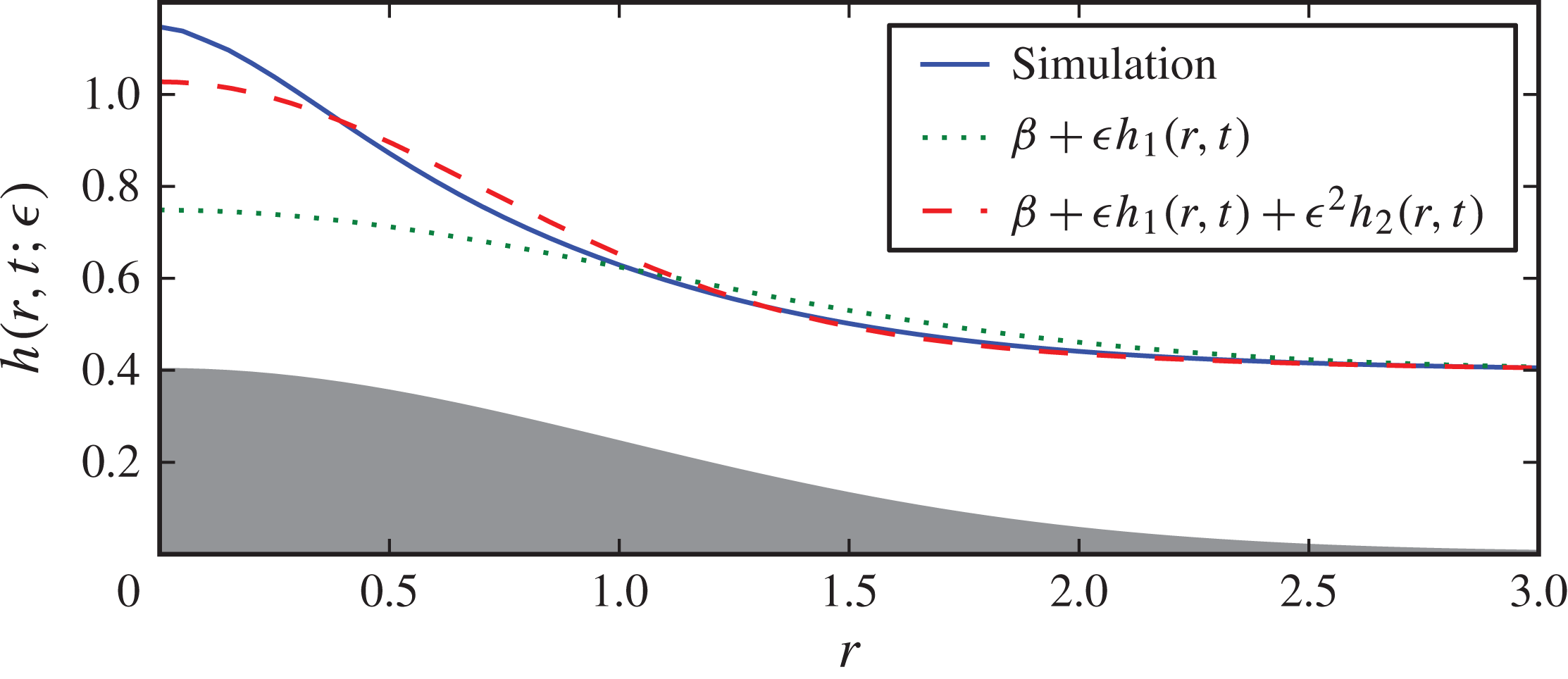
The radial dependence of the free-surface deformation
 $h(r,t;{\it\epsilon})$
at
 $t=10$
is plotted in figure 12, comparing simulation results to domain-perturbation solutions. The
 $O({\it\epsilon})$
solution has reached a steady state at this point and is plotted to demonstrate that the
 $O({\it\epsilon}^{2})$
contribution is crucial to the dynamics. In addition, the comparison of profiles from the simulation and the
 $O({\it\epsilon}^{2})$
domain-perturbation solution reveals that the acceleration of the jet growth is due to a narrowing and steepening of the profile. Despite these differences that inevitably arise at late times, the
 $O({\it\epsilon}^{2})$
domain-perturbation solution captures the early-time behaviour well and gives a reasonable estimate for the initial jet velocity, even at this large value of
 ${\it\epsilon}$
.
Comparison of axisymmetric domain-perturbation surface profiles with simulated profiles for
 ${\it\beta}=0.4$
and
 ${\it\epsilon}=0.4$
at
 $t=10$
. The solid curve (blue online) denotes the simulation result, the dotted curve (green online) denotes the
 $O({\it\epsilon})$
domain-perturbation solution
 ${\it\epsilon}h_{1}(r,t)$
, and the dashed curve (red online) denotes the
 $O({\it\epsilon}^{2})$
solution
 ${\it\epsilon}h_{1}(r,t)+{\it\epsilon}^{2}h_{2}(r,t)$
. The grey shape shows the maximum blister deformation. The error in the
 $O({\it\epsilon})$
solution demonstrates that the
 $O({\it\epsilon}^{2})$
contribution is crucial to the dynamics.

8. Implications for BA-LIFT
The boundary deformation observed in BA-LIFT experiments can be approximated by the functional form
 $$\begin{eqnarray}\bar{h}_{b}(\bar{r},\bar{t})=H_{b}(E)\left[1-\left(\frac{\bar{r}}{R_{b}(E)}\right)^{2}\right]^{1.25}F(\bar{t}),\end{eqnarray}$$
where the blister height
 $H_{b}$
and radius
 $R_{b}$
increase with laser pulse energy
 $E$
; the time evolution is given approximately by
 $$\begin{eqnarray}F(\bar{t})=\frac{2}{{\rm\pi}}\arctan \left(\frac{\bar{t}}{{\it\tau}_{B}}\right),\end{eqnarray}$$
with
 ${\it\tau}_{B}=23.6~\text{ns}$
(Brown et al.
Reference Brown, Brasz, Ventikos and Arnold2012). These empirical fits were used in Brown et al. (Reference Brown, Brasz, Ventikos and Arnold2012) in volume-of-fluid simulations of the Navier–Stokes equations to investigate the threshold laser energy required to transfer a droplet as a function of various fluid properties. To apply the domain-perturbation results to these BA-LIFT transfers, the blister radius
 $R_{b}$
needs to be converted to an effective Gaussian width
 $c$
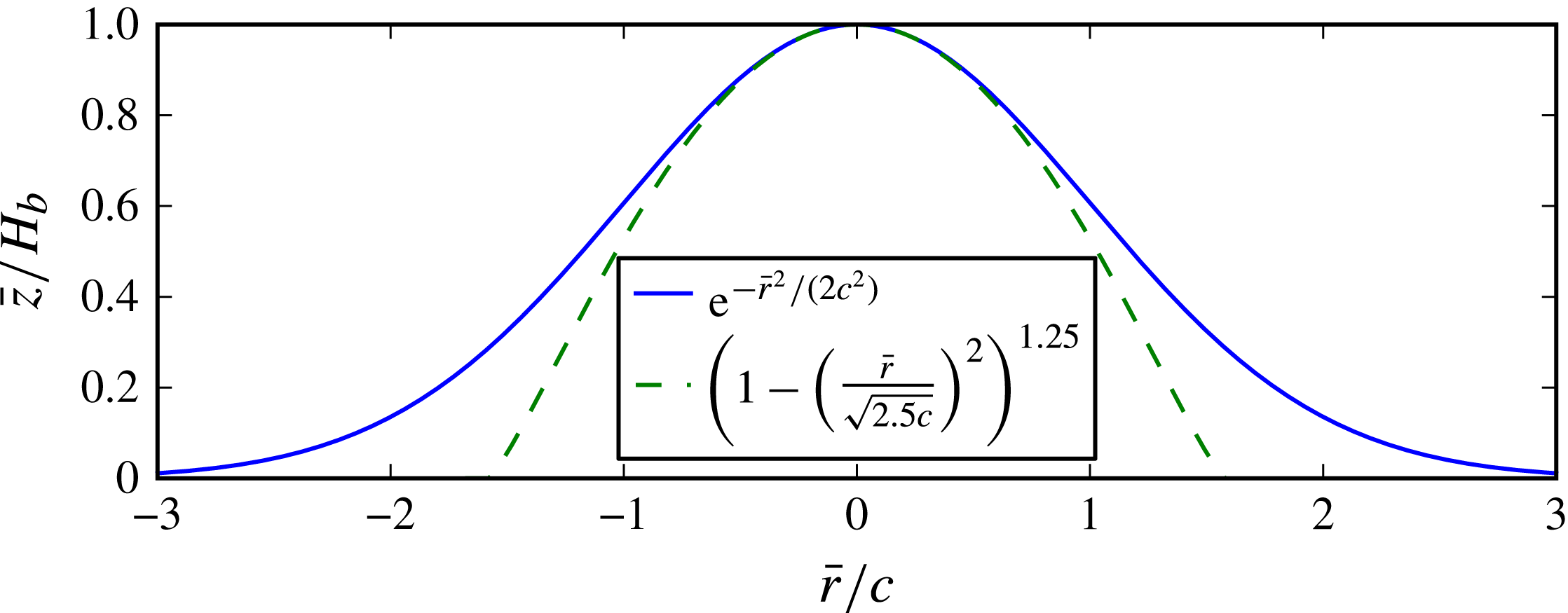
. Figure 13 shows that taking
 $R_{b}=\sqrt{2.5}c$
makes the deformations match fairly well in the central region, with equal curvatures at
 $r=0$
. Thus, non-dimensionalizing by the length scale
 $c=R_{b}(E)/\sqrt{2.5}$
allows one to compute effective values for
 ${\it\epsilon}$
and
 ${\it\beta}$
given
 $E$
and
 $H$
. Table 3 provides some examples of parameters corresponding to blisters formed at various pulse energies in the simulations of Brown et al. (Reference Brown, Brasz, Ventikos and Arnold2012).


Blister parameters and corresponding length scales and non-dimensional values given a laser pulse energy
 $E$
and film thickness
 $H=5~{\rm\mu}\text{m}$
. Here
 $c=R_{b}/\sqrt{2.5}$
is the length scale used for non-dimensionalization. The upper bound
 $r_{d}^{\ast }$
on the radius of a drop that could be produced by the deformation is calculated using (8.4) with
 ${\it\rho}=1030~\text{kg}~\text{m}^{-3}$
,
 ${\it\gamma}=40.8~\text{mN}~\text{m}^{-1}$
and
 ${\it\tau}=37~\text{ns}$
. A typical drop radius
 $R_{b}/3$
is included for comparison to
 $r_{d}^{\ast }$
.

The difference between the time evolution (8.2) used in Brown et al. (Reference Brown, Brasz, Ventikos and Arnold2012) and the simple exponential decay used earlier can also be taken into account. After non-dimensionalizing time in (8.2) by
 ${\it\tau}_{B}$
and differentiating, we can calculate
 $\int _{0}^{\infty }f^{2}(t)\text{d}t=1/{\rm\pi}$
. Recalling (4.7) and the fact that
 $\int _{0}^{\infty }\text{e}^{-2t}\text{d}t=1/2$
, we then choose
 ${\it\tau}=({\rm\pi}/2){\it\tau}_{B}\approx 37$
ns instead of
 ${\it\tau}_{B}$
as the time scale for non-dimensionalization in order to make the quantitative results for the domain-perturbation remnant flow apply to the BA-LIFT simulations.
An initial check that we can carry out with this mapping from
 $E$
and
 $H$
to
 ${\it\epsilon}$
and
 ${\it\beta}$
is to examine the remnant kinetic energy as a function of
 $E$
at fixed
 $H$
. This can be compared with figure 11(b) of Brown et al. (Reference Brown, Brasz, Ventikos and Arnold2012), in which the (dimensional) kinetic energy at 300 ns (
 $t\approx 8.1$
) is plotted versus
 $E-E_{th}$
at
 $H=5$
, where
 $E_{th}=3.65~{\rm\mu}\text{J}$
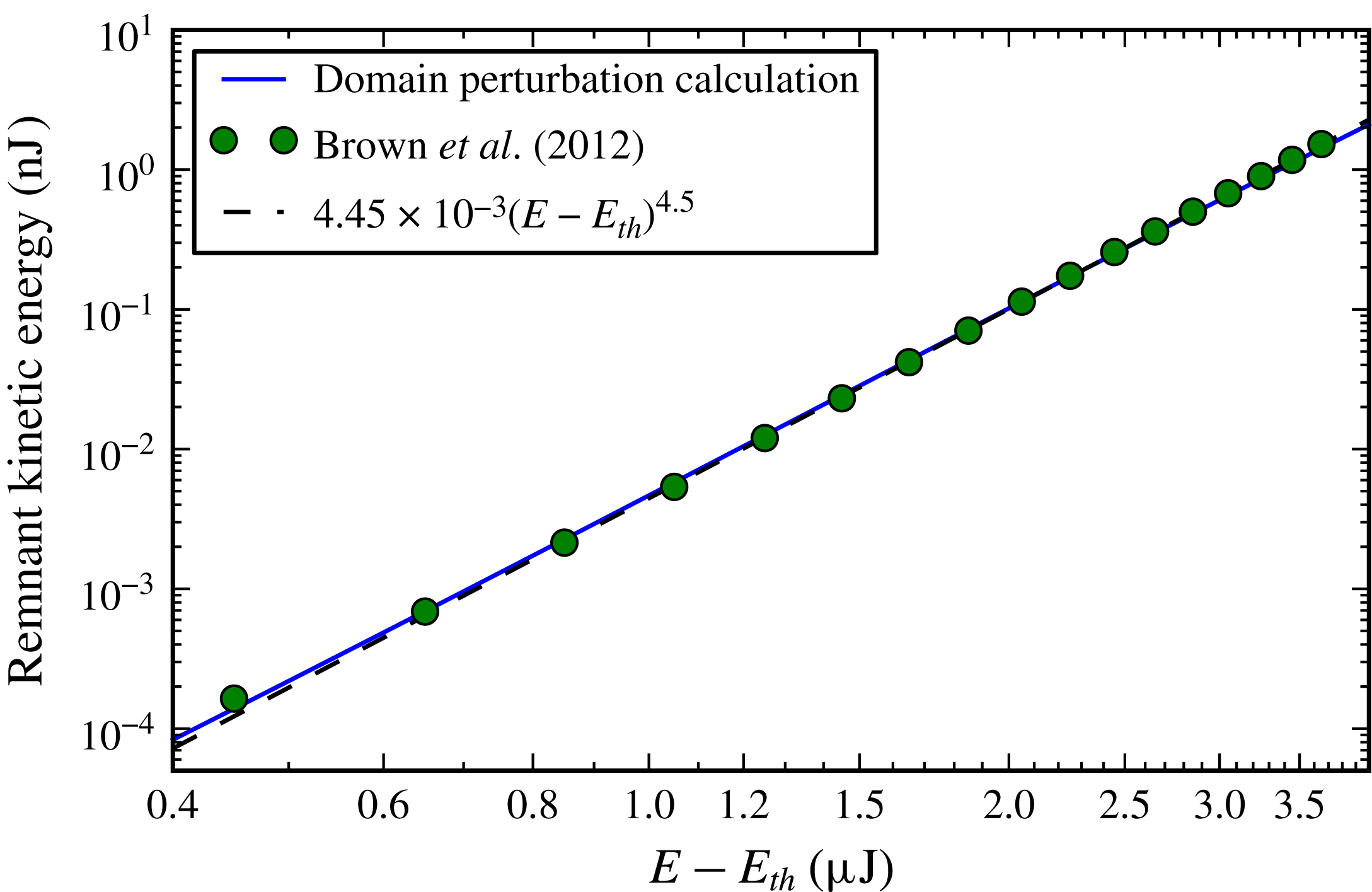
is the threshold energy for blister formation. Figure 14 combines those data with the remnant kinetic energy calculated from the domain perturbation and dimensionalized by
 ${\it\rho}c^{5}/{\it\tau}^{2}$
, showing excellent agreement with the simulation data and the fit from Brown et al. (Reference Brown, Brasz, Ventikos and Arnold2012). As the full numerical simulations included viscosity and surface tension, this agreement verifies that the initial transfer of energy in BA-LIFT is indeed dominantly inertial and that the axisymmetric domain-perturbation approach captures the energy transfer quantitatively.
Remnant kinetic energy in the fluid from axisymmetric domain-perturbation calculations,
 $\bar{E}_{k}(\infty )$
, compared to total kinetic energy in the full simulations of Brown et al. (Reference Brown, Brasz, Ventikos and Arnold2012) at 300 ns (
 $t\approx 8.1$
) and its corresponding fit, as a function of laser energy above the threshold for blister formation,
 $E_{th}=3.65~{\rm\mu}\text{J}$
. The film thickness is fixed at
 $H=5~{\rm\mu}\text{m}$
, and the parameters
 ${\it\epsilon}$
and
 ${\it\beta}$
are obtained from the empirical fits
 $H_{b}(E)$
and
 $R_{b}(E)$
from Brown et al. (Reference Brown, Brasz, Ventikos and Arnold2012) together with
 $c=R_{b}/\sqrt{2.5}$
. The remnant kinetic energy from the domain-perturbation calculation is dimensionalized by
 ${\it\rho}c^{5}/{\it\tau}^{2}$
, with
 ${\it\rho}=1030~\text{kg}~\text{m}^{-3}$
and
 ${\it\tau}=37~\text{ns}$
.

The remaining kinetic energy in the fluid after the boundary motion stops can be related to jet formation by considering surface energy. Surface tension will oppose the formation of a jet, and, if the kinetic energy in the fluid is too low, the jet will retract back into the liquid layer. There is a threshold energy at which the jet forms a drop, and, for higher energies, the velocity of the jet increases and a larger volume of liquid is transferred (Brown et al.
Reference Brown, Brasz, Ventikos and Arnold2012). We can estimate how this threshold for fluid transfer depends on the problem parameters by assuming that all kinetic energy is converted to surface energy of the drop. The condition that a drop of radius
 $r_{d}$
can be produced is then that
 $$\begin{eqnarray}\bar{E}_{k}\geqslant \bar{E}_{s}=4{\rm\pi}r_{d}^{2}{\it\gamma},\end{eqnarray}$$
where
 ${\it\gamma}$
is the surface tension.
Substituting the dimensional form of (6.4) for
 $\bar{E}_{k}$
for times
 $t\gg 1$
, the upper bound
 $r_{d}^{\ast }$
on the radius of a drop that might be produced is
 $$\begin{eqnarray}r_{d}^{\ast }=c{\it\epsilon}^{2}\sqrt{\frac{\mathit{We }\,\hat{E}_{k,4}({\it\beta})}{4{\rm\pi}}},\end{eqnarray}$$
where
 $\mathit{We}\equiv {\it\rho}U^{2}L/{\it\gamma}={\it\rho}c^{3}/{\it\gamma}{\it\tau}^{2}$
is the Weber number. For the BA-LIFT simulations in Brown et al. (Reference Brown, Brasz, Ventikos and Arnold2012), the fluid properties used were those of the liquid NMP, which has
 ${\it\gamma}=40.8~\text{mN}~\text{m}^{-1}$
,
 ${\it\rho}=1030~\text{kg}~\text{m}^{-3}$
and
 ${\it\mu}=1.7~\text{mPa}~\text{s}$
. The corresponding values of
 $\mathit{We}$
and
 $r_{d}^{\ast }$
are included in table 3. The drop radius is not known a priori, but simulations of BA-LIFT suggest that the drop radius increases with both blister radius and film thickness and typically falls in the range
 $R_{b}/10$
to
 $R_{b}/2$
(Brown et al.
Reference Brown, Brasz, Ventikos and Arnold2012). As an approximation, then, a typical drop radius
 $R_{b}/3$
can be compared with
 $r_{d}^{\ast }$
. If
 $r_{d}^{\ast }\ll R_{b}/3$
, no drop will be produced by the blister; and if
 $r_{d}^{\ast }\gg R_{b}/3$
, the jet will have sufficient energy to pinch off into one or more drops. An approximate threshold for pinch-off is given by
 $r_{d}^{\ast }=R_{b}/3$
, and
 $R_{b}/3$
is included in table 3. The blister from a
 $4.5~{\rm\mu}\text{J}$
pulse does not leave enough kinetic energy in a
 $5~{\rm\mu}\text{m}$
thick film to eject a droplet, as it does not satisfy
 $r_{d}^{\ast }>R_{b}/3$
, but the higher laser energies do, so they are expected to produce droplets. Indeed,
 $5.1~{\rm\mu}\text{J}$
is the threshold laser energy to transfer a droplet from a
 $5~{\rm\mu}\text{m}$
thick film, and the radius predicted by volume-of-fluid simulations is
 $r_{d}\approx 5.4~{\rm\mu}\text{m}$
(Brown et al.
Reference Brown, Brasz, Ventikos and Arnold2012), which is close to the estimate
 $R_{b}/3\approx 5.5~{\rm\mu}\text{m}$
. The difference between
 $r_{d}^{\ast }\approx 6.9~{\rm\mu}\text{m}$
and
 $r_{d}$
can be attributed to viscous losses and residual surface and kinetic energies after pinch-off.
We can examine other simulation results from Brown et al. (Reference Brown, Brasz, Ventikos and Arnold2012) to check if this result holds as parameters are varied. For a
 $10~{\rm\mu}\text{m}$
thick film, the threshold laser energy is approximately
 $5.7~{\rm\mu}\text{J}$
, which corresponds to
 ${\it\epsilon}=0.43$
,
 ${\it\beta}=0.85$
and
 $r_{d}^{\ast }=10.2~{\rm\mu}\text{m}$
. This is consistent with producing a droplet of radius
 $R_{b}/3=6.2~{\rm\mu}\text{m}$
, again leaving some extra energy. The large
 ${\it\beta}$
resulting from this thicker film means that a
 $5.1~{\rm\mu}\text{J}$
laser pulse would only leave enough energy to produce a hypothetical droplet of radius
 $r_{d}^{\ast }=4.3~{\rm\mu}\text{m}$
, so
 $5.1~{\rm\mu}\text{J}$
is clearly below the threshold laser energy for this film thickness.
Alternatively, the results from the domain-perturbation calculation can be used to predict the optimum film thickness given other blister parameters. Taking the blister corresponding to a
 $5.1~{\rm\mu}\text{J}$
laser pulse with its length scale
 $c=10.5~{\rm\mu}\text{m}$
, the optimum film thickness for transferring kinetic energy to the liquid layer is given by
 $H=c{\it\beta}_{k}\approx 3.7~{\rm\mu}\text{m}$
. One could also optimize the velocity of the forming jet,
 $v_{2}(0,{\it\beta},\infty )$
, by taking
 $H=c{\it\beta}_{v}\approx 4.0~{\rm\mu}\text{m}$
. The film thickness that minimizes threshold laser energy in figure 17 of Brown et al. (Reference Brown, Brasz, Ventikos and Arnold2012) lies between 2.5 and
 $5~{\rm\mu}\text{m}$
, so these values of
 $3.7$
or
 $4.0~{\rm\mu}\text{m}$
are in agreement. Furthermore, the domain-perturbation results reveal that viscosity is not required to explain why the threshold laser energy for transfer increases as the film thickness decreases below the critical value.
9. Discussion
In this paper we have shown that the deformation of a flat solid boundary into a bump protruding into an initially quiescent liquid layer induces a fluid flow that can lead to jet formation. While the solid boundary is deforming, the liquid layer deforms with it. The velocity field is in the direction of the solid boundary deformation and also laterally outwards from the bump. As the boundary motion slows and approaches its final shape, kinetic energy is removed from the liquid, yet a flow remains. This remnant flow is still in the direction of the bump, but the lateral motion has reversed. The slowing of the boundary leads to a low-pressure region just above the bump, and liquid is drawn in towards the centre from the surrounding fluid. It is this inward flow that can lead to jet formation and is the basis of the laser-induced printing technique BA-LIFT.
A domain-perturbation method for
 ${\it\epsilon}\ll 1$
, where
 ${\it\epsilon}=kH_{b}/2$
(or
 $H_{b}/c$
in the axisymmetric case) is the effective aspect ratio of the solid boundary deformation, was used to obtain an asymptotic solution for the velocity field in this boundary-driven fluid flow. At leading order,
 $O({\it\epsilon})$
, the slowing of the boundary deformation towards a steady state eliminates all fluid motion; but at
 $O({\it\epsilon}^{2})$
, a remnant flow is found, arising from the nonlinear interaction between the solid boundary motion and the free surface. This remnant flow is inwards towards the crest of the deformation and perpendicular to the free surface at the crest.
The dimensional velocity after the boundary motion stops scales as
 ${\it\epsilon}^{2}/k{\it\tau}=H_{b}^{2}k/{\it\tau}$
, with a
 ${\it\beta}$
dependence that has a maximum at
 ${\it\beta}_{v}\approx 0.706$
and decreases as
 $\text{e}^{-{\it\beta}}$
for large
 ${\it\beta}$
, where
 ${\it\beta}=kH$
is proportional to the ratio of the layer thickness to the radius of the solid deformation. The total kinetic energy (per unit width into the page) remaining in the fluid after the deformation scales as
 ${\it\rho}{\it\epsilon}^{4}/(k^{4}{\it\tau}^{2})={\it\rho}H_{b}^{4}/{\it\tau}^{2}$
, with a
 ${\it\beta}$
dependence that reaches a maximum at
 ${\it\beta}_{k}\approx 0.611$
and decays as
 $\text{e}^{-2{\it\beta}}$
for large
 ${\it\beta}$
. These results are independent of the temporal evolution
 $f(t)$
and suggest that
 ${\it\beta}\approx 0.6{-}0.7$
may be optimal for forming a strong liquid jet, with the other parameters held fixed. In general, we see that jet velocities can be increased by decreasing the time scale for boundary deformation
 ${\it\tau}$
, increasing the maximum boundary displacement
 $H_{b}$
, or choosing a layer thickness to make
 ${\it\beta}$
closer to
 ${\it\beta}_{v}$
. The effect of increasing
 $k$
and using a narrower deformation is more complex because both
 ${\it\epsilon}$
and
 ${\it\beta}$
change, but if
 ${\it\beta}<{\it\beta}_{v}$
, increasing
 $k$
will increase the jet velocity.
The domain-perturbation solution is extended from two dimensions to an axisymmetric formulation with a Gaussian boundary deformation replacing the sinusoidal deformation of the 2D case. The same qualitative results apply, with
 $1/c$
replacing
 $k$
as the length scale and an energy scale of
 ${\it\rho}c^{5}{\it\epsilon}^{4}/{\it\tau}^{2}$
. Quantitatively, the critical values for
 ${\it\beta}$
are
 ${\it\beta}_{v}\approx 0.384$
and
 ${\it\beta}_{k}\approx 0.354$
in the axisymmetric case, and the remnant kinetic energy decays as
 $\text{e}^{-2.5{\it\beta}}$
for large
 ${\it\beta}$
. These critical values of
 ${\it\beta}$
are not directly comparable to the values from the 2D case, as the Gaussian and sinusoidal boundary deformations have differing characteristic widths. By replacing the sinusoidal functional form by
 $[1+\cos (x\sqrt{2}/c)]/2$
, it matches the Gaussian form (6.1) in the same manner as figure 13, with equal curvatures at
 $x=0$
. With this rescaled sinusoidal boundary deformation, the critical values of
 ${\it\beta}=H/c$
in the 2D case would be a factor of
 $\sqrt{2}$
smaller, or
 ${\it\beta}_{v}\approx 0.499$
and
 ${\it\beta}_{k}\approx 0.432$
, closer to the axisymmetric values.
Numerical simulations confirm the domain-perturbation results and test their limits for larger
 ${\it\epsilon}$
in the axisymmetric case. Velocity slices from simulations have similar forms to the domain-perturbation results for
 ${\it\epsilon}\lesssim 0.4$
at
 $t=t^{\ast }+5$
, with vertical stretching and focusing at
 $r=0$
significant for larger values of
 ${\it\epsilon}$
. The time evolution of the free surface was investigated in § 7.3, showing an initial period of time when the deformation of the solid boundary rapidly deforms the free surface according to the
 $O({\it\epsilon})$
solution, followed by a later period when the domain-perturbation results predict that the remaining
 $O({\it\epsilon}^{2})$
velocity field continues to deform the free surface at a constant rate, increasing the length of the forming jet. This agrees well at smaller
 ${\it\epsilon}$
, but, at the rather large
 ${\it\epsilon}=0.4$
relevant for drop formation, numerical simulations reveal that the jet narrows and begins to accelerate beyond the
 $O({\it\epsilon}^{2})$
remnant jet speed around the transition time
 $t^{\ast }$
, given by (6.5). The domain-perturbation results still provide a reasonable estimate for jet velocity, however, and non-zero surface tension will eventually stop this inertial acceleration anyway.
The remnant kinetic energy transferred to the fluid predicted by the axisymmetric domain-perturbation results shows excellent agreement with previous simulations of BA-LIFT after converting blister parameters to an effective Gaussian width and time constant. The conversion of the remnant kinetic energy into surface energy was used to make a simple estimate (8.4) of the threshold for drop formation.
The effects of surface tension and viscosity are insignificant on the time scale of the solid boundary deformation in BA-LIFT and hence are appropriately neglected, so our results reveal the early-time dynamics of the purely inertial free-surface flow driven by a deforming solid boundary. These dynamics are crucial to understanding the nature of the induced jet.
Acknowledgements
The authors gratefully acknowledge financial support for this research from the National Science Foundation MRSEC program through the Princeton Center for Complex Materials (grant DMR-0819860).
Supplementary movie
A supplementary movie is available at http://dx.doi.org/10.1017/jfm.2015.74.
Appendix A. Axisymmetric domain-perturbation solution
The boundary conditions (3.6) and (3.7) at the free surface are unchanged from the 2D case after making the substitutions
 $x\rightarrow r$
and
 $y\rightarrow z$
and defining
 $u$
and
 $v$
as radial and vertical velocities, respectively. At
 $z=0$
, the kinematic conditions replacing (3.5) are
 $$\begin{eqnarray}\displaystyle v_{1}=\text{e}^{-r^{2}/2}f(t), & & \displaystyle\end{eqnarray}$$
 $$\begin{eqnarray}\displaystyle v_{2}=-F(t)\text{e}^{-r^{2}/2}\left(ru_{1}+\frac{\partial v_{1}}{\partial z}\right). & & \displaystyle\end{eqnarray}$$
A.1. The
$O({\it\epsilon})$
solution

Consider a solution for
 ${\it\phi}_{1}$
of the form given in (6.3), with coefficients
 $A_{1}(k,t)$
and
 $B_{1}(k,t)$
. The boundary velocity (A 1a
) decays to zero for large
 $r$
, so
 $C(t)=0$
. The dynamic condition (3.6a
) requires that
 $A_{1}(k,t)=0$
, and the kinematic condition (A 1a
) leads to
 $$\begin{eqnarray}-\int _{0}^{\infty }B_{1}(k,t)\cosh {\it\beta}k\,J_{0}(kr)k\text{d}k=\text{e}^{-r^{2}/2}f(t).\end{eqnarray}$$
The Hankel transform of
 $\text{e}^{-r^{2}/2}$
is
 $\text{e}^{-k^{2}/2}$
, so the solution for
 $B_{1}(k,t)$
is given by
 $$\begin{eqnarray}B_{1}(k,t)=f(t)\hat{B}_{1}(k)=-f(t)\text{e}^{-k^{2}/2}/\cosh {\it\beta}k.\end{eqnarray}$$
The
 $O({\it\epsilon})$
velocity potential and components can then be written as
 $$\begin{eqnarray}\displaystyle {\it\phi}_{1}(r,z,t) & = & \displaystyle -f(t)\int _{0}^{\infty }\text{e}^{-k^{2}/2}\frac{\sinh [k({\it\beta}-z)]}{\cosh {\it\beta}k}J_{0}(kr)\text{d}k,\end{eqnarray}$$
 $$\begin{eqnarray}\displaystyle u_{1}(r,z,t) & = & \displaystyle f(t)\int _{0}^{\infty }\text{e}^{-k^{2}/2}\frac{\sinh [k({\it\beta}-z)]}{\cosh {\it\beta}k}J_{1}(kr)k\text{d}k,\end{eqnarray}$$
 $$\begin{eqnarray}\displaystyle v_{1}(r,z,t) & = & \displaystyle f(t)\int _{0}^{\infty }\text{e}^{-k^{2}/2}\frac{\cosh [k({\it\beta}-z)]}{\cosh {\it\beta}k}J_{0}(kr)k\text{d}k.\end{eqnarray}$$
 $h_{1}(r,t)=\int _{0}^{t}v_{1}(r,{\it\beta},s)\text{d}s$
, we find
 $$\begin{eqnarray}h_{1}(r,t)=F(t)\int _{0}^{\infty }\frac{\text{e}^{-k^{2}/2}}{\cosh {\it\beta}k}J_{0}(kr)k\text{d}k.\end{eqnarray}$$
A.2. The
$O({\it\epsilon}^{2})$
solution for
$t\gg 1$


We begin by supposing a solution of the form (6.3) for
 ${\it\phi}_{2}$
, now with coefficients
 $A_{2}(k,t)$
and
 $B_{2}(k,t)$
, and again taking
 $C(t)=0$
. The dynamic condition (3.6b
) at the free surface leads to
 $$\begin{eqnarray}\int _{0}^{\infty }\frac{\partial A_{2}(k,t)}{\partial t}J_{0}(kr)\text{d}k=-\!\left({\dot{f}}F+\frac{\,f^{2}}{2}\right)\left(\int _{0}^{\infty }\hat{B}_{1}(k)J_{0}(kr)k\text{d}k\right)^{2},\end{eqnarray}$$
which clearly has a separable solution
 $A_{2}(k,t)=\hat{A}_{2}(k)a(t)$
, where
 $$\begin{eqnarray}\int _{0}^{\infty }\hat{A}_{2}(k)J_{0}(kr)\text{d}k=\left(\int _{0}^{\infty }\hat{B}_{1}(k)J_{0}(kr)k\text{d}k\right)^{2}=\left(\frac{v_{1}(r,{\it\beta},t)}{f(t)}\right)^{2}\equiv \hat{v}_{1}^{2}(r,{\it\beta})\end{eqnarray}$$
and
 $$\begin{eqnarray}a(t)=-f(t)F(t)+\frac{1}{2}\int _{0}^{t}f^{2}(s)\text{d}s.\end{eqnarray}$$
The transform (A 7) must be solved for numerically for a given
 ${\it\beta}$
by computing
 $$\begin{eqnarray}\hat{A}_{2}(k)=k\int _{0}^{\infty }\hat{v}_{1}^{2}(r,{\it\beta})J_{0}(kr)r\text{d}r.\end{eqnarray}$$
The equation for the time dependence
 $a(t)$
is analogous to that in (3.21) for
 ${\dot{a}}_{n}(t)$
in the 2D case, and at long times we again use
 $f(t)\rightarrow 0$
and define
 $$\begin{eqnarray}a_{\infty }\equiv \lim _{t\rightarrow \infty }a(t)=\frac{1}{2}\int _{0}^{\infty }f^{2}(t)\text{d}t.\end{eqnarray}$$
For example,
 $a_{\infty }=1/4$
for
 $f(t)=\text{e}^{-t}$
.
The solid boundary condition (A 1b ) can be written as
 $$\begin{eqnarray}\displaystyle & & \displaystyle \int _{0}^{\infty }[A_{2}(k,t)\sinh {\it\beta}k+B_{2}(k,t)\cosh {\it\beta}k]J_{0}(kr)k\text{d}k\nonumber\\ \displaystyle & & \displaystyle \quad =f(t)F(t)\text{e}^{-r^{2}/2}\int _{0}^{\infty }\text{e}^{-k^{2}/2}\tanh {\it\beta}k\,[rJ_{1}(kr)-kJ_{0}(kr)]k\text{d}k.\end{eqnarray}$$
For
 $t\gg 1$
, the boundary deformation stops and
 $f(t)\rightarrow 0$
, leaving
 $$\begin{eqnarray}\lim _{t\rightarrow \infty }B_{2}(k,t)=-\text{tanh}({\it\beta}k)\hat{A}_{2}(k)a_{\infty }.\end{eqnarray}$$
The remnant velocity potential and components at long times can then be written as
 $$\begin{eqnarray}\displaystyle {\it\phi}_{2}(r,z,\infty ) & = & \displaystyle a_{\infty }\int _{0}^{\infty }\hat{A}_{2}(k)\left\{\cosh [k({\it\beta}-z)]\right.\nonumber\\ \displaystyle & & \displaystyle \left.-\tanh {\it\beta}k\sinh [k({\it\beta}-z)]\right\}J_{0}(kr)\text{d}k,\end{eqnarray}$$
 $$\begin{eqnarray}\displaystyle u_{2}(r,z,\infty ) & = & \displaystyle -a_{\infty }\int _{0}^{\infty }\hat{A}_{2}(k)\left\{\cosh [k({\it\beta}-z)]\right.\nonumber\\ \displaystyle & & \displaystyle \left.-\tanh {\it\beta}k\sinh [k({\it\beta}-z)]\right\}J_{1}(kr)k\text{d}k,\end{eqnarray}$$
 $$\begin{eqnarray}\displaystyle v_{2}(r,z,\infty ) & = & \displaystyle -a_{\infty }\int _{0}^{\infty }\hat{A}_{2}(k)\left\{\sinh [k({\it\beta}-z)]\right.\nonumber\\ \displaystyle & & \displaystyle \left.-\tanh {\it\beta}k\cosh [k({\it\beta}-z)]\right\}J_{0}(kr)k\text{d}k.\end{eqnarray}$$
A.3. Time-dependent
$O({\it\epsilon}^{2})$
solution

With further similar calculations, one can obtain the time-dependent
 $O({\it\epsilon}^{2})$
solution as
 $$\begin{eqnarray}\displaystyle {\it\phi}_{2}(r,z,t) & = & \displaystyle \int _{0}^{\infty }\left\{A_{2}(k,t)\cosh [k({\it\beta}-z)]\right.\nonumber\\ \displaystyle & & \displaystyle \left.+\,B_{2}(k,t)\sinh [k({\it\beta}-z)]\right\}J_{0}(kr)\text{d}k,\end{eqnarray}$$
 $$\begin{eqnarray}\displaystyle B_{2}(k,t) & = & \displaystyle \frac{{\hat{C}}_{2}(k)}{\cosh {\it\beta}k}\,f(t)F(t)-A_{2}(k,t)\tanh {\it\beta}k,\end{eqnarray}$$
 $$\begin{eqnarray}\displaystyle {\hat{C}}_{2}(k) & = & \displaystyle \int _{0}^{\infty }R_{2}(r)J_{0}(kr)r\text{d}r,\end{eqnarray}$$
 $$\begin{eqnarray}\displaystyle R_{2}(r) & = & \displaystyle \text{e}^{-r^{2}/2}\int _{0}^{\infty }\text{e}^{-k^{2}/2}\tanh {\it\beta}k\,[rJ_{1}(kr)-kJ_{0}(kr)]k\text{d}k.\end{eqnarray}$$
 $b_{n}(t)$
has the transient contribution
 $-[\tanh {\it\beta}/(n\cosh n{\it\beta})]\,f(t)F(t)$
in (3.20). For
 $t\gg 1$
,
 $f(t)$
approaches zero and this term dies out, as does the
 $[{\hat{C}}_{2}(k)/\cosh {\it\beta}k]\,f(t)F(t)$
term, leaving the constant remnant solution found earlier.
The free-surface deformation can be solved using (3.16), or
 $$\begin{eqnarray}\frac{\partial h_{2}}{\partial t}(r,t)=-\int _{0}^{\infty }B_{2}(k,t)J_{0}(kr)k\text{d}k.\end{eqnarray}$$
Integrating the time dependences leads to
 $$\begin{eqnarray}h_{2}(r,t)=\int _{0}^{\infty }\left[\left(a_{\infty }t-\frac{1}{2}F^{2}(t)\right)\hat{A}_{2}(k)\tanh {\it\beta}k-\frac{1}{2}F^{2}(t)\frac{{\hat{C}}_{2}(k)}{\cosh {\it\beta}k}\right]J_{0}(kr)k\text{d}k.\end{eqnarray}$$
At long times,
 $h_{2}(r,t)$
grows linearly with time, and we recover
 $$\begin{eqnarray}\frac{\partial h_{2}}{\partial t}(r,\infty )=v_{2}(r,{\it\beta},\infty )=a_{\infty }\int _{0}^{\infty }\hat{A}_{2}(k)\tanh ({\it\beta}k)J_{0}(kr)k\text{d}k.\end{eqnarray}$$
Appendix B. Numerical method
The finite-difference scheme is derived by transforming Laplace’s equation from Cartesian coordinates
 $(x,y)$
to curvilinear coordinates
 $({\it\xi},{\it\eta})$
with the mapping
 $$\begin{eqnarray}x={\it\xi},\quad y=h_{b}({\it\xi},t)+q({\it\xi},t){\it\eta},\end{eqnarray}$$
where
 $h_{b}({\it\xi},t)$
is the boundary displacement, as before, and
 $q({\it\xi},t)$
is a scaling factor for cell heights such that
 $n_{y}$
evenly spaced grid points extend from the solid to the free surface at all values of
 $x$
; figure 15 shows a mesh after the solid boundary has finished deforming for
 ${\it\beta}=0.7$
and
 ${\it\epsilon}=0.2$
. The curvilinear coordinate values remain constant and uniformly spaced throughout the simulation, with
 $n_{x}$
points in the range
 $-{\rm\pi}\leqslant {\it\xi}\leqslant {\rm\pi}$
and
 $n_{y}$
points in the range
 $0\leqslant {\it\eta}\leqslant {\it\beta}$
. Only the
 $y$
values of grid points change with time, and these changes are captured in the time dependence of
 $h_{b}({\it\xi},t)$
and
 $q({\it\xi},t)$
.
Grid used for numerical simulations with
 ${\it\epsilon}=0.2$
and
 ${\it\beta}=0.7$
at
 $t=20$
. The coordinate
 ${\it\xi}$
is constant along vertical grid lines, and
 ${\it\eta}$
(defined in (B 1)) is constant along the curves going left to right.

Appendix C contains details on the discretization of Laplace’s equation in the curvilinear coordinate system, which results in a sparse linear system of equations of the form
 $\unicode[STIX]{x1D63C}{\bf\phi}=\boldsymbol{b}$
. After initializing the domain to be a Cartesian grid on
 $[-{\rm\pi},{\rm\pi}]\times [0,{\it\beta}]$
with
 $q({\it\xi},0)=1$
, the numerical procedure for each time step of duration
 ${\rm\Delta}t$
is as follows:
-
(i) Iteratively solve the linear system of equations for
${\it\phi}$
at all interior grid points with successive over-relaxation, using periodicity in the
$x$
direction and a Dirichlet condition at
${\it\eta}={\it\beta}$
, keeping
${\it\phi}$
fixed. Before each iteration of the linear solver, the
${\it\eta}=0$
boundary condition
$\partial {\it\phi}/\partial n=n_{y}V_{b}(x,t)$
must be applied. This is done by discretizing (B 2)using central differences in
$$\begin{eqnarray}\frac{\partial {\it\phi}}{\partial n}=n_{x}\frac{\partial {\it\phi}}{\partial x}+n_{y}\frac{\partial {\it\phi}}{\partial y}=n_{x}\left(\frac{\partial {\it\xi}}{\partial x}\frac{\partial {\it\phi}}{\partial {\it\xi}}+\frac{\partial {\it\eta}}{\partial x}\frac{\partial {\it\phi}}{\partial {\it\eta}}\right)+n_{y}\left(\frac{\partial {\it\xi}}{\partial y}\frac{\partial {\it\phi}}{\partial {\it\xi}}+\frac{\partial {\it\eta}}{\partial y}\frac{\partial {\it\phi}}{\partial {\it\eta}}\right)\end{eqnarray}$$
${\it\xi}$
and one-sided second-order differences in
${\it\eta}$
, leading to an inner linear system of equations to update
${\it\phi}$
along
${\it\eta}=0$
.
-
(ii) Advance in time the grid points on the free surface by advecting them according to the velocity field and updating
${\it\phi}$
with the Lagrangian form of (2.3b
), that is,
$\text{D}{\it\phi}/\text{D}t=(u^{2}+v^{2})/2$
. -
(iii) Interpolate to obtain
$y$
and
${\it\phi}$
values of new grid points equally spaced in
${\it\xi}$
.


This sequence of steps is used with a second-order Runge–Kutta time integrator and a time step between 0.001 and 0.1, depending on
 ${\it\epsilon}$
. The solver for Laplace’s equation is validated against simple test cases with analytical solutions to ensure that the discretization in curvilinear coordinates is performed correctly, and Dirichlet and Neumann boundary conditions are applied correctly on curved boundaries.
B.1. Extension to axisymmetric domains
The finite-difference method is extended to solve for axisymmetric flows by making the substitutions
 $x\rightarrow r$
and
 $y\rightarrow z$
. The coordinates
 ${\it\xi}$
and
 ${\it\eta}$
are still defined as in (B 1), with
 $n_{r}$
points in the range
 $0\leqslant {\it\xi}\leqslant 6$
and
 $n_{z}$
points in the range
 $0\leqslant {\it\eta}\leqslant {\it\beta}$
for the Gaussian boundary deformation (6.2). Figure 16 shows a mesh after the solid boundary has finished deforming for
 ${\it\beta}=0.4$
and
 ${\it\epsilon}=0.4$
.
Grid used for axisymmetric numerical simulations with
 ${\it\epsilon}=0.4$
and
 ${\it\beta}=0.4$
at
 $t=10$
.

A symmetry boundary condition must now be applied at
 ${\it\xi}=0$
before each iteration of the linear solver. This is the Neumann condition
 $\partial {\it\phi}/\partial n=\partial {\it\phi}/\partial r=0$
, which is solved in a similar fashion to the boundary condition
 ${\it\eta}=0$
in the 2D case. This Neumann condition is also applied at
 ${\it\xi}=6$
, where velocities are negligible.
Most of the results of appendix C still hold, with the modification that each
 $B^{ij}$
is multiplied by the corresponding value of
 $r$
. This change arises because, in cylindrical coordinates, Laplace’s equation can be written as
 $$\begin{eqnarray}{\rm\nabla}^{2}{\it\phi}=\frac{1}{r}\left[\frac{\partial }{\partial r}\left(r\frac{\partial {\it\phi}}{\partial r}\right)+\frac{\partial }{\partial z}\left(r\frac{\partial {\it\phi}}{\partial z}\right)\right]=0,\end{eqnarray}$$
so, by inspection of (C 1),
 $B^{ij}$
can absorb the extra factor
 $r$
for cylindrical coordinates. As the coordinate transformation (B 1) does not change
 $r$
values, this simple modification works for transformed cylindrical coordinates as well. The solver is again validated against simple test cases, checking Dirichlet and Neumann conditions with curved and stretched domains.
Appendix C. Discretization of Laplace’s equation
With the coordinate transformation (B 1),
 ${\rm\nabla}^{2}{\it\phi}=0$
becomes
 $$\begin{eqnarray}{\rm\nabla}^{2}{\it\phi}=\frac{1}{J}\frac{\partial }{\partial {\it\xi}_{j}}\left(\frac{B^{kj}}{J}\frac{\partial {\it\phi}}{\partial {\it\xi}_{k}}\right),\end{eqnarray}$$
where
 $B^{kj}={\it\beta}^{ik}{\it\beta}^{ij}$
,
 ${\it\beta}^{ij}$
is the cofactor of
 $\partial x_{i}/\partial {\it\xi}_{j}$
in the matrix
 $$\begin{eqnarray}\unicode[STIX]{x1D648}=\left[\begin{array}{@{}cc@{}}{\displaystyle \frac{\partial x}{\partial {\it\xi}}} & {\displaystyle \frac{\partial x}{\partial {\it\eta}}}\\ {\displaystyle \frac{\partial y}{\partial {\it\xi}}} & {\displaystyle \frac{\partial y}{\partial {\it\eta}}}\end{array}\right]\end{eqnarray}$$
and
 $J=\det (\unicode[STIX]{x1D648})$
is the Jacobian determinant of the transformation (Ferziger & Perić Reference Ferziger and Perić2002). We can thus find in two dimensions that
 $$\begin{eqnarray}\displaystyle B^{11} & = & \displaystyle \left(\frac{\partial y}{\partial {\it\eta}}\right)^{2}+\left(\frac{\partial x}{\partial {\it\eta}}\right)^{2},\end{eqnarray}$$
 $$\begin{eqnarray}\displaystyle B^{21} & = & \displaystyle B^{12}=-\frac{\partial y}{\partial {\it\xi}}\frac{\partial y}{\partial {\it\eta}}-\frac{\partial x}{\partial {\it\xi}}\frac{\partial x}{\partial {\it\eta}},\end{eqnarray}$$
 $$\begin{eqnarray}\displaystyle B^{22} & = & \displaystyle \left(\frac{\partial y}{\partial {\it\xi}}\right)^{2}+\left(\frac{\partial x}{\partial {\it\xi}}\right)^{2}.\end{eqnarray}$$
A Cartesian mesh with a nine-point stencil in
 $({\it\xi},{\it\eta})$
space is used to discretize (C 1). Referring to a central point
 ${\it\phi}(i{\rm\Delta}{\it\xi},j{\rm\Delta}{\it\eta})={\it\phi}_{i,j}$
as
 ${\it\phi}_{P}$
, neighbouring points on the mesh can be described as
 ${\it\phi}_{E}$
,
 ${\it\phi}_{NE}$
,
 ${\it\phi}_{N}$
,
 ${\it\phi}_{NW}$
,
 ${\it\phi}_{W}$
,
 ${\it\phi}_{SW}$
,
 ${\it\phi}_{S}$
and
 ${\it\phi}_{SE}$
, where for example
 ${\it\phi}_{NW}={\it\phi}_{i-1,j+1}$
. Lower-case subscripts in
 ${\it\phi}_{e}$
,
 ${\it\phi}_{n}$
,
 ${\it\phi}_{w}$
and
 ${\it\phi}_{s}$
denote values halfway between grid points.
Starting with the discretization of the inner derivatives, (C 1) becomes
 $$\begin{eqnarray}\displaystyle {\rm\nabla}^{2}{\it\phi}=0 & = & \displaystyle \frac{\partial }{\partial {\it\xi}}\left[\frac{1}{J}\left(\frac{{\it\phi}_{e}-{\it\phi}_{w}}{{\rm\Delta}{\it\xi}}B^{11}+\frac{{\it\phi}_{N}-{\it\phi}_{S}}{2{\rm\Delta}{\it\eta}}B^{21}\right)\right]\nonumber\\ \displaystyle & & \displaystyle +\,\frac{\partial }{\partial {\it\eta}}\left[\frac{1}{J}\left(\frac{{\it\phi}_{E}-{\it\phi}_{W}}{2{\rm\Delta}{\it\xi}}B^{12}+\frac{{\it\phi}_{n}-{\it\phi}_{s}}{{\rm\Delta}{\it\eta}}B^{22}\right)\right].\end{eqnarray}$$
Discretizing the outer derivatives then yields
 $$\begin{eqnarray}\displaystyle 0 & = & \displaystyle \frac{1}{\left({\rm\Delta}{\it\xi}\right)^{2}}\left[\left(\frac{B^{11}}{J}\right)_{e}({\it\phi}_{E}-{\it\phi}_{P})-\left(\frac{B^{11}}{J}\right)_{w}({\it\phi}_{P}-{\it\phi}_{W})\right]\nonumber\\ \displaystyle & & \displaystyle +\,\frac{1}{4{\rm\Delta}{\it\xi}{\rm\Delta}{\it\eta}}\left[\left(\frac{B^{21}}{J}\right)_{E}({\it\phi}_{NE}-{\it\phi}_{SE})-\left(\frac{B^{21}}{J}\right)_{W}({\it\phi}_{NW}-{\it\phi}_{SW})\right]\nonumber\\ \displaystyle & & \displaystyle +\,\frac{1}{4{\rm\Delta}{\it\xi}{\rm\Delta}{\it\eta}}\left[\left(\frac{B^{12}}{J}\right)_{N}({\it\phi}_{NE}-{\it\phi}_{NW})-\left(\frac{B^{12}}{J}\right)_{S}({\it\phi}_{SE}-{\it\phi}_{SW})\right]\nonumber\\ \displaystyle & & \displaystyle +\,\frac{1}{\left({\rm\Delta}{\it\eta}\right)^{2}}\left[\left(\frac{B_{22}}{J}\right)_{n}({\it\phi}_{N}-{\it\phi}_{P})-\left(\frac{B_{22}}{J}\right)_{s}({\it\phi}_{P}-{\it\phi}_{S})\right].\end{eqnarray}$$
We now have an algebraic system of equations that can be written as
 $$\begin{eqnarray}\mathop{\sum }_{d}A_{d}{\it\phi}_{d}=0\end{eqnarray}$$
for each direction
 $d$
. It is solved with a successive over-relaxation method with a relaxation factor
 ${\it\omega}=1.925$
, which was found to work well in reducing solution times.