INTRODUCTION
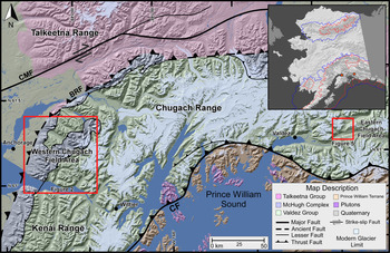
The Chugach Mountains in south-central Alaska, stretching for >400 km, represent one of the most accessible areas in Alaska and have some of the best-preserved glacial geologic evidence for the region (Fig. 1). However, the timing of past glaciations in this region has not been well defined in previous studies. The Chugach Mountains were the locus of the western extent of the Cordilleran ice sheet during the last glacial period, which oscillated several times and is dated to the marine isotope stages [MIS] 5d through 2 (Karlstrom, Reference Karlstrom1964; Briner and Kaufman, Reference Briner and Kaufman2008). Extant glaciation is restricted to intermittent ice fields and valley glaciers that advance into Prince William Sound and the adjacent lowlands (Fig. 1).
Digital elevation model showing major faults and geologic terranes of south-central Alaska. The red boxes outline the detailed field areas of this project. The inset map of Alaska depicts a simplified maximum extent of glaciation during the Pleistocene (blue) and the late Wisconsinan (red). The orange points represent the locations of the field areas in this study. The base map for the inset is modified from Riehle (Reference Riehle2011). BRF, Border Ranges Fault; CF, Contact Fault; CMF, Castle Mountain Fault. (For interpretation of the references to color in this figure legend, the reader is referred to the web version of this article.)

Karlstrom (Reference Karlstrom1961, Reference Karlstrom1964) was the first to develop the glacial history for Anchorage and the Cook Inlet in the Chugach Mountain region. He identified a succession of Wisconsinan moraines that he suggested were formed during MIS 2. Radiocarbon dating of the older moraines in this region was partially successful in estimating the minimum ages of glaciation (Table 1). Complications related to the radiocarbon age calibration and less-advanced analytical techniques available during the 1960s did not allow Karlstrom (Reference Karlstrom1964) to define glaciation timing adequately. At that time, radiocarbon dating required large bulk sediment samples, which introduced considerable uncertainty and error due to carbon contamination from the presence of subbituminous and lignitic coal derived from the underlying geologic formations (Reger et al., Reference Reger, Sturmann, Berg and Burns2007). Since the original work of Karlstrom (Reference Karlstrom1964), the glacial history has been intensively studied and outlined by Schmoll and Yehle (Reference Schmoll, Yehle, Hamilton, Reed and Thorson1986), Schmoll et al. (Reference Schmoll, Yehle and Updike1999), Calkin et al. (Reference Calkin, Wiles and Barclay2001), and Reger et al. (Reference Reger, Sturmann, Berg and Burns2007). However, there has been no thorough study using modern techniques to date a complete sequence of early (~MIS 4) and late Wisconsin glaciations in the Chugach Mountains.
Calibrated radiocarbon ages (ka) for the four stadials of the Naptowne glaciation as summarized by Reger et al. (Reference Reger, Sturmann, Berg and Burns2007). The name provided in parentheses for each measured age range under each stade are those used by that specific author for that local glacial event and may differ from the overarching stadial definitions adopted here.

Reconstructing the timing and extent of glaciation in south-central Alaska helps test the synchronicity of glaciation between maritime and continental regions of the western margins of the Northern American ice sheets during the late Quaternary. This, in turn, helps in understanding regional and global synchronicity of climatic and glacial history, essential for testing and developing models for past and future climate change. In addition, the Chugach Mountains provide new data on early Wisconsinan glaciation that are lacking for many regions of the world. Our study encompasses two main study areas, Williwaw Lakes and Thompson Pass, both on the edges of the higher-altitude yet accessible portions of the Chugach Mountains. The Williwaw Lakes region, a deglaciated and low-elevation valley located on the western side of the Chugach Mountains near Anchorage (Fig. 1), contains an impressive assemblage of presumed early Wisconsinan glaciated surfaces and late Wisconsinan moraines. This area was selected because it likely contains a complete succession of late Wisconsinan moraines. Study of this succession of moraines will contribute to the currently sparse dating throughout south-central Alaska. The Thompson Pass region in the eastern Chugach Mountains near the town of Valdez lies nearly 200 km to the east of Anchorage (Fig. 1) and on a plateau of high topography containing active glaciers and glacially polished bedrock steps, moraines, and boulders. The Thompson Pass site was selected because it was generally accessible and is located in the core of the Chugach Mountains, where no dating had been previously undertaken. We use 10Be and 36Cl terrestrial cosmogenic nuclides to develop glacial chronostratigraphies for these two regions and compare them with the timing of glaciation across Alaska to understand better regional variations and possible climate forcing factors.
Regional setting
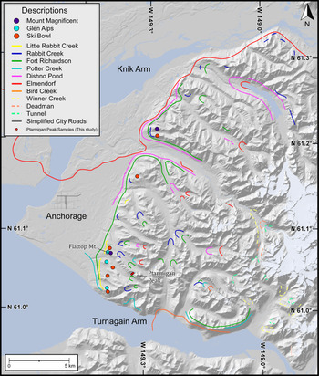
The Chugach Mountains are a product of accretion in the Late Cretaceous and oblique collision and subduction of the Yakutat microplate since the Oligocene (Plafker, Reference Plafker, Scholl, Grantz and Vedder1987; Bruhn and Haeussler, Reference Bruhn and Haeussler2006; Abers, Reference Abers, Freymueller, Haeussler, Wesson and Ekström2008; Fuis et al., Reference Fuis, Moore, Plafker, Brocher, Fisher, Mooney and Nokleberg2008; Haeussler, Reference Haeussler, Freymueller, Haeussler, Wesson and Ekström2008; Finzel et al., Reference Finzel, Trop, Ridgway and Enkelmann2011). Their topography is rugged and rises to 4016 m above sea level (m asl) at Mount Marcus Baker, whereas the deepest valleys drop to sea level (Buscher et al., Reference Buscher, Berger, Spotila, Freymueller, Haeussler, Wesson and Ekström2008). Loci of high glaciated topography correspond to zones of rapid exhumation in the core of the Chugach Mountains north of Prince William Sound (Arkle et al., Reference Arkle, Armstrong, Haeussler, Prior, Hartman, Sendziak and Brush2013) and north of the Bagley Icefield in the St. Elias Mountains (Berger and Spotila, Reference Berger and Spotila2008; Berger et al., Reference Berger, Spotila, Chapman, Pavlis, Enkelmann, Ruppert and Buscher2008). The majority of the Chugach Mountains have been extensively glaciated throughout the Quaternary, oscillating from total coverage to interspersed valley glaciers that advanced from ice fields across the center of the range (Fig 1). Currently, the ice fields and valley glaciers are comparatively smaller than the surrounding regions, and many of the valleys are unglaciated in the western side of the Chugach Mountains. This study area's landscapes typically comprise a complex assemblage of moraines, glaciated bedrock surfaces, and outwash deposits (Schmoll et al., Reference Schmoll, Yehle and Updike1999; Fig. 2). Both late and early Wisconsinan glacial landforms and sediments are typically well-preserved, because Holocene glaciers in the western Chugach Mountains did not advance more than ~0.5–2 km downvalley from the location of modern glaciers.
A shaded relief map (produced from a 10-m-elevation DEM) showing the regional distribution and relative chronologies of moraines in the Anchorage and Chugach Mountain regions (adapted from Schmoll et al., Reference Schmoll, Yehle and Updike1999). Large dots represent early Wisconsinan till located on small flat surfaces. The colored lines represent late Wisconsinan moraines, glacial trimlines, outer edges of till deposits, and former ice-flow markers. (For interpretation of the references to color in this figure legend, the reader is referred to the web version of this article.)

The Quaternary glaciations of south-central Alaska and the Cook Inlet are controlled by strong climatic gradients and high relief and steep slopes. South-central Alaska and the Chugach Mountains are warmer and wetter today than elsewhere in Alaska, due to the maritime climate and orographic precipitation derived from southeasterly winds advecting moisture from the Pacific Ocean (Reger et al., Reference Reger, Sturmann, Berg and Burns2007). The average annual precipitation for the Chugach Mountains’ windward side is currently ~1800 mm, while the landward continental interior side of the Chugach Mountains is colder and has an average annual precipitation of ~500 mm (National Climate Data Center, 2007).
Quaternary glacial record in the Chugach Mountains
Radiocarbon, cosmogenic nuclide, and lichenometry ages for moraines in Alaska date to the early last glacial period (early Wisconsinan), late last glacial period (late Wisconsinan), and the Holocene (Karlstrom, Reference Karlstrom1964; Briner et al., Reference Briner, Kaufman, Manley, Finkel and Caffee2005, 2017; Briner and Kaufman, Reference Briner and Kaufman2008; Dortch et al., Reference Dortch, Owen, Caffee and Brease2010a, 2010b; Solomina et al., Reference Solomina, Bradley, Hodgson, Ivy-Ochs, Jomelli, Mackintosh and Nesje2015; Kaufman et al., Reference Kaufman, Axford, Henderson, McKay, Oswald, Saenger and Anderson2016; Menounos et al., Reference Menounos, Goehring, Osborn, Margold, Ward, Bond and Clarke2017). Reconstructions and dating of moraines consistently indicate that glaciers in Alaska reached their most recent maximum extent during the early Wisconsinan (Kaufman and Manley, Reference Kaufman and Manley2004; Briner and Kaufman, Reference Briner and Kaufman2008; Dortch et al., Reference Dortch, Owen, Caffee, Li and Lowell2010b; Kaufman et al., Reference Kaufman, Young, Briner, Manley, Ehlers and Gibbard2011, Briner et al., Reference Briner, Tulenko, Kaufman, Young, Baichtal and Lesnek2017). This early maximum glacial advance contrasts with the maximum global ice volumes that occurred during the global last glacial maximum (gLGM), as defined by Mix et al. (Reference Mix, Bard and Schneider2001) at ~24–18 ka, Clark et al. (Reference Clark, Dyke, Shakun, Carlson, Clark, Wohlfarth, Mitrovica, Hostetler and McCabe2009) at ~26–19 ka, and Hughes and Gibbard (Reference Hughes and Gibbard2015) at ~28–23 ka. As in other mountain glacial systems throughout the world (Thackray et al., Reference Thackray, Owen and Yi2008; Schaefer et al., Reference Schaefer, Putnam, Denton, Kaplan, Birkel, Doughty and Kelly2015), regional climatic factors in Alaska favored glacier growth during the early Wisconsinan compared with the late Wisconsinan (Briner and Kaufman, Reference Briner and Kaufman2008). In Alaska, the early Wisconsinan glaciation has been defined by a few numerical dating studies of glacial landforms and sediments from major mountain ranges at 60–50 ka; these include studies by Briner et al. (Reference Briner, Kaufman, Manley, Finkel and Caffee2005), Ward et al. (Reference Ward, Bond and Gosse2007), Briner and Kaufman (Reference Briner and Kaufman2008), Dortch et al. (Reference Dortch, Owen, Caffee, Li and Lowell2010b), Kaufman et al. (Reference Kaufman, Young, Briner, Manley, Ehlers and Gibbard2011), and Tulenko et al. (Reference Tulenko, Briner, Young and Schaefer2018). We refer to these glaciations as the local last glacial maximum (lLGM), as the maximum extent of glaciation was not coincident with the gLGM, and the timing may be different slightly between study areas.
The Wisconsinan glaciations were first correlated by Karlstrom (Reference Karlstrom1958, Reference Karlstrom1964) and regionally defined in southern Alaska as the Naptowne glaciation. The Naptowne glaciation has four stades that were dated using radiocarbon methods, and the recalibrated ages include the Moose Horn (32–25 ka), Killey (19.5–18.5 ka), Skilak (18.0–17.0 ka), and Elmendorf (15.0–11.0 ka) stades. Except for the Elmendorf stade, the ages for these stades outside southern Alaska are poorly defined by a few radiocarbon ages and tephrochronology (Karlstrom, Reference Karlstrom1958, Reference Karlstrom1964; Schmoll and Dobrovolny, Reference Schmoll and Dobrovolny1972; Schmoll and Yehle, Reference Schmoll, Yehle, Hamilton, Reed and Thorson1986; Reger and Updike, Reference Reger and Updike1983; Mann and Peteet, Reference Mann and Peteet1994; Reger et al., Reference Reger, Pinney, Burke and Wiltse1996, 2007; Stilwell and Kaufman, Reference Stilwell and Kaufman1996; Reger and Pinney, Reference Reger, Pinney, Karl, Vaughn and Ryherd1997; Schmoll et al., Reference Schmoll, Yehle and Updike1999; Ager, Reference Ager, Kelley and Gough2000; Table 1). The work of Kopczynski et al. (Reference Kopczynski, Kelley, Lowell, Evenson and Applegate2017) firmly established a complete chronology of the retreat of the Matanuska-Knik glacial lobe ranging in recalibrated ages at ~17.5–11.5 ka (known as the Elmendorf stade).
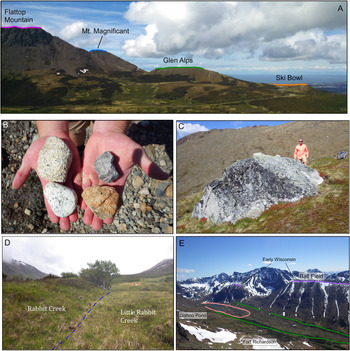
Evidence for early Wisconsinan glacial advances in the Chugach Mountains include erratics and scattered till deposits draped over glacially polished mountaintops and saddles above late Wisconsinan glacial trimlines (Schmoll et al., Reference Schmoll, Yehle and Updike1999; Fig. 2). The oldest recorded glacial surfaces are attributed to the regional Susitna glaciation. Evidence for this glaciation is preserved on the highest glacier-scoured mountaintops and steps at an elevation of ~1070 m asl (Fig. 3). Three consecutively younger early Wisconsinan glacial advances are characterized by till draped over glacially polished flat steps (oldest to youngest: Mount Magnificent, Glen Alps, and Ski Bowl), which are best preserved along the western side of Flattop Mountain (Schmoll et al., Reference Schmoll, Yehle and Updike1999; Fig 4A). These glaciations were probably related to the large valley glaciers in the Susitna River valley and Cooke Inlet that advanced from the Alaska Range and Talkeetna Mountains (Figs. 1 and 2).
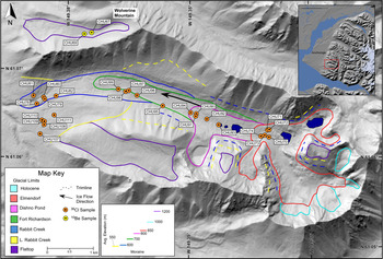
(color online) Glacial geomorphology of Williwaw Lakes valley showing the glacial limits (outermost end or lateral moraine and/or outermost till deposit) and sample locations.

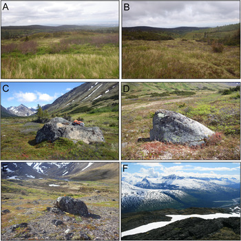
Views of significant landforms in Williwaw Lakes valley and Thompson Pass study areas. (A) A profile view of the Flattop Mountain and early Wisconsinan surfaces that correlate with (from top to bottom) the Mount Susitna, Mount Magnificent, Glen Alps, and Ski Bowl glacial advances (Schmoll et al., Reference Schmoll, Yehle and Updike1999). (B) A comparison of early Wisconsinan clasts composed of granite (left) and locally derived late Wisconsinan moraine clast composed of metasedimentary volcaniclastics (right). (C) Granitic glacial boulder located below Wolverine Peak (CHU67). (D) View of the contact (dashed blue line) between the Rabbit Creek (right) and Little Rabbit Creek (left) moraines. (E) View of Williwaw Lakes valley showing Fort Richardson lateral moraines and the flat glaciated benches above the valley. (For interpretation of the references to color in this figure legend, the reader is referred to the web version of this article.)

No previous Quaternary glacial chronostratigraphy has been developed for the Thompson Pass area of the eastern Chugach Mountains, but the landforms and glacial limits were mapped by Moffit (Reference Moffit1935) and Péwé (Reference Péwé1975). During the lLGM, most of this region likely was covered by glaciers, as indicated by the deep U-shaped valleys, fresh glacially polished bedrock, notch canyons, and isolated arêtes (Moffit, Reference Moffit1935; Fig. 4). Glaciers are still present in the area due to higher annual precipitation (~3300 mm/yr at Thompson Pass; Western Regional Climate Center, 2016) compared with the drier (~400 mm/yr at Anchorage; Western Regional Climate Center, 2016) western parts of the Chugach Mountains.
Description of study areas
In this study, early Wisconsinan glacier-eroded surfaces in the western Chugach Mountains were mapped below Ptarmigan Peak (Fig. 2), on Flattop Mountain (Fig. 4A), and above Williwaw Lakes valley (Fig. 3). At Flattop Mountain, there are four flat steps at various elevations (from lowest to highest: Ski Bowl, Glen Alps, Mount Magnificent, and Flattop Mountain summit), which are blanketed in till and have scattered erratics (Fig. 4A). At the Ptarmigan Peak site, a saddle-shaped surface with hummocky moraine and erratics was present midway up the mountain at an elevation of ~1100 m asl (Supplementary Fig. 1). Above Williwaw Lakes valley, four flat steps (Wolverine Peak, the Ball Field, below O'Malley Peak, and below Williwaw Peak) are present on flat-topped ridges residing at a similar height of ~200 m above the glacial trimlines of the younger late Wisconsinan glacial advances (Fig. 3).
Late Wisconsinan moraines in the Williwaw Lakes valley have variable characteristics depending upon the altitude. The low-elevation moraines contain small and eroded glacial boulders overgrown by brush. The higher-elevation moraines have sparse vegetation, and large boulders are more abundant. Vegetation obscures any small-scale glacial features, and significant erosion has resulted in the moraines having a subdued morphology. These factors strongly affect the surface morphology of the Little Rabbit and Rabbit Creek moraines (Figs. 4D and 5A). The Rabbit Creek advance consists of an end moraine and discontinuous lateral moraines (Fig. 3), where the end moraine is an ~5-m-high ridge adjacent to the Little Rabbit Creek moraines (Figs. 4D and 5B). The Fort Richardson end moraine is discontinuous where it crosses the center of the valley, but is well-preserved along the sides of the valley, and ranges in height from ~5 to 8 m (Figs. 3, 4E, and 5C). The Dishno Pond end moraine is ~2 m high and protrudes from the marsh-like interior of the Fort Richardson moraine (Fig. 3). This moraine is relatively younger and is at a slightly higher elevation; hummocks and kame terraces, paternoster lakes, and flat gravel deposits are present on the moraine surface (Figs. 3 and 5D). The Elmendorf end moraine is at the head of the valley (Fig. 3), and a thin veneer of till interspersed with roche moutonnées ranging in height from ~1 to 3 m is present through the landscape. Thicker deposits of moraine and hummocks that range in height from ~2 to 6 m are present at the downstream end of the Elmendorf moraine (Fig. 5E).
(color online) Views of the five moraines in Williwaw Lakes valley and the incised steps of Thompson Pass study areas. The surface of Little Rabbit Creek (A), Little Rabbit (B), Fort Richardson (C), Dishno Pond (D), and Elmendorf (E) moraines. (F) View from Thompson Pass depicting the large glacial steps and the notch canyons.

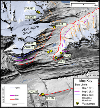
The Thompson Pass region generally has three broad (1- to 10-km-wide) discontinuous and glacially scoured bedrock steps (Figs. 6 and 5F). We call these steps S1, S2, and S3, and they occur at elevations of 600, 800, and 1200 m asl, respectively (Fig. 6). S1 is a series of east-west trending bedrock ridges that range in height from ~5 to 10 m. The S2 step is an ~3- to 15-m-high east trending glacially polished bedrock surface, with ~2- to 4-m-diameter glacial boulders on its flattest surfaces. The exposed bedrock on S1 and S2 has well-preserved p-forms, striations, and chatter marks. S3 is a glacially polished bedrock surface with roche moutonnées, small ponds, and streams.
A shaded relief map of Thompson Pass showing glaciation trimlines and sampling locations. The red, purple, and blue lines represent the glacial trimlines for three Pleistocene glaciations. The orange lines represent the ice maximum during the Holocene. The grayish-blue color represents the modern ice extent. (For interpretation of the references to color in this figure legend, the reader is referred to the web version of this article.)

METHODS
Mapping and sampling approach
We remapped the moraines described by Schmoll et al. (Reference Schmoll, Yehle and Updike1999) in the Williwaw Lakes area using 90-m-resolution digital elevation models (DEMs) and Google Earth imagery (Image © 2015 DigitalGlobe and U.S. Geological Survey), including five early Wisconsinan surfaces and four late Wisconsinan moraines. We recorded in the field the surficial characteristics and spatial limits of moraines and glacial trimlines in both the Williwaw Lakes valley and Thompson Pass regions.
We attempted to date five moraines and four distinct elevation levels having bedrock steps covered in glacial debris. Our sites were selected based on accessibility and the presence of glacial boulders and datable glacially polished bedrock surfaces. Samples for 10Be and 36Cl surface exposure age dating were collected from erratics, glacial boulders, and glacially eroded bedrock surfaces throughout both study areas. Fifteen granitic or quartz-rich samples were analyzed for 10Be and 25 samples were processed for 36Cl. Thirty-three of the samples were composed of sandstone, shale, and metasedimentary rocks locally sourced from the Chugach Group (Plafker et al., Reference Plafker, Nokleberg and Lull1989). The remaining seven samples were composed of granite, presumably sourced from the Talkeetna Mountains to the north of the field area (Fig. 1).
In the Williwaw Lakes area, we sampled and dated all five moraines of the late Wisconsinan glacier advance and early Wisconsinan glacial boulders and glacially polished bedrock surfaces from the flat top of Flattop Mountain, a saddle below Ptarmigan Peak, and a sloped surface below Wolverine Peak (Figs. 3 and 4A). In the western Chugach site at Thompson Pass, samples for dating were collected from glacial boulders and glacially polished bedrock to define the ages of three glacially eroded steps (Fig. 6).
Approximately 500 g of rock were collected from a measured thickness (1–7 cm deep) of the top of each sampled surface using a hammer and chisel. We aimed to quantify the sampled moraines’ ages by collecting from five glacial boulders for each moraine and one to three samples of erratics or the glacially eroded bedrock surfaces. The size and shape of the boulders and the geometry of the resting surface were used to help assess whether the boulders were stable since deposition. The largest possible glacial boulders and erratics were chosen, because they were least likely to have moved or been obscured by vegetation after deposition compared with unstable, smaller, and low-lying glacial boulders. Boulder sizes were recorded, and photographs were taken for all samples and their geologic context (Supplementary Fig. 2).
Several sampling environmental and geologic factors may introduce reliability and consistency problems for TCN (Terrestrial Cosmogenic Nuclide) dating (Hallet and Putkonen, Reference Hallet and Putkonen1994; Benn and Owen, Reference Benn and Owen2002; Seong et al., Reference Seong, Owen, Bishop, Bush, Clendon, Copland, Finkel, Kamp and Shroder2007; Heyman et al, Reference Heyman, Stroeven, Harbor and Caffee2011, Owen et al., Reference Owen, Chen, Hedrick, Caffee, Robinson, Schoenbohm, Yuan, Li, Imrecke and Liu2012). Physical shielding due to snow and sediment, weathering of the sampled surfaces, and exhumation reduce the concentration of TCNs from the surface, resulting in an underestimated age. Conversely, exposure of boulders to cosmic rays before deposition would result in overestimates of the age of the landform. Glacial boulders and erratics that are small, flush with the ground surface, or very old are more prone to these factors, which is the case for many of the samples from the early Wisconsinan surfaces and oldest moraine sets (e.g., Little Rabbit Creek and Rabbit Creek). Although we consider it worthwhile to measure and report these ages, we recognize the need for caution in interpreting them due to the problems of using low-lying boulders in potentially unstable settings. Details on the distribution of these ages and how they are used to contribute to the glacial history of the region are addressed in the “Discussion.”
All dated till deposits were physically characterized using pebble counts to roughly determine clast provenance. We used a variant of Wolman's pebble count method (Wolman, Reference Wolman1954; Sampson and Smith, Reference Sampson and Smith2006), in which we measured the intermediate axis, angularity, and composition of 100 clasts collected at 0.5 m increments along 50-m-long lines across deposits or surfaces at each location (Supplementary Table 1).
10Be and 36Cl dating
Sample processing and chemical analysis for 10Be and 36Cl dating were conducted in the geochronology laboratories at the University of Cincinnati. For 10Be dating, each sample was crushed and sieved to 250–500 μm. Quartz was separated from each sample following the methods of Kohl and Nishizumi (Reference Kohl and Nishizumi1992). Each sample was spiked with low-background Be carrier that was prepared by Abaz Alimanovic at the University of Melbourne, who dissolved beryl collected from a deep mine. 10Be was separated and purified by ion-exchange chromatography and precipitated as Be(OH)2 at pH > 7. The Be(OH)2 was combusted by ignition in quartz crucibles, producing BeO. The BeO was mixed with Nb metal before being loaded into steel carriers.
Methods for sample preparation and isolation of 36Cl follow the procedures of Stone et al. (Reference Stone, Allan, Fifield and Cresswell1996). Samples were crushed and sieved down to <250 μm to obtain 250 g of material, and then the samples were leached in HNO3 to remove contaminants and eliminate meteoric 36Cl. An ~10 g aliquot was separated from the sample and sent to Bureau Veritas Mineral Laboratories in Vancouver, Canada, for major trace element analysis using Inductively Coupled Plasma Mass Spectrometry (ICP-MS) (Supplementary Table 2). A 30 g sample was dissolved in an HF/HNO3 solution and spiked with ~1.0 mg enriched 35Cl. After dissolution, fluoride compounds were isolated through centrifuging, and AgNO3 and HNO3 were added to precipitate AgCl. AgCl was collected and dissolved in NH4OH, and Cl was subsequently extracted through anion-exchange chromatography. AgCl was finally precipitated with the addition of AgNO3 and HNO3 and loaded into Cu cathodes. Accelerator mass spectrometry analysis for 10Be and 36Cl was undertaken at the Purdue Rare Isotope Measurement (PRIME) Laboratory at Purdue University.
Ages were calculated using CRONUScalc (Marrero et al., Reference Marrero, Phillips, Borchers, Lifton, Aumer and Balco2015a), a web calculator that incorporates the globally calibrated production rates of Marrero et al. (Reference Marrero, Phillips, Caffee and Gosse2015b; Table 2). We chose the scaling factors of Lal (Reference Lal1991), Stone (Reference Stone2000), and Lifton et al. (Reference Lifton, Sato and Dunai2014) for comparison (Tables 2 and 3). The Young et al. (Reference Young, Schaefer, Briner and Goehring2013) 10Be sea-level high-altitude production rate calibration (3.96 ± 0.15 atoms/g SiO2/yr) was chosen for these calculations, because it best represents high-latitude environments and is most comparable to the field area (Baffin Island). For comparison of the TCN ages with the literature data, all radiocarbon ages from prior studies were recalibrated using the online software OxCal v. 4.4, utilizing the IntCal 20 curve (Ramsey et al., Reference Ramsey, van der Plicht and Weninger2001).
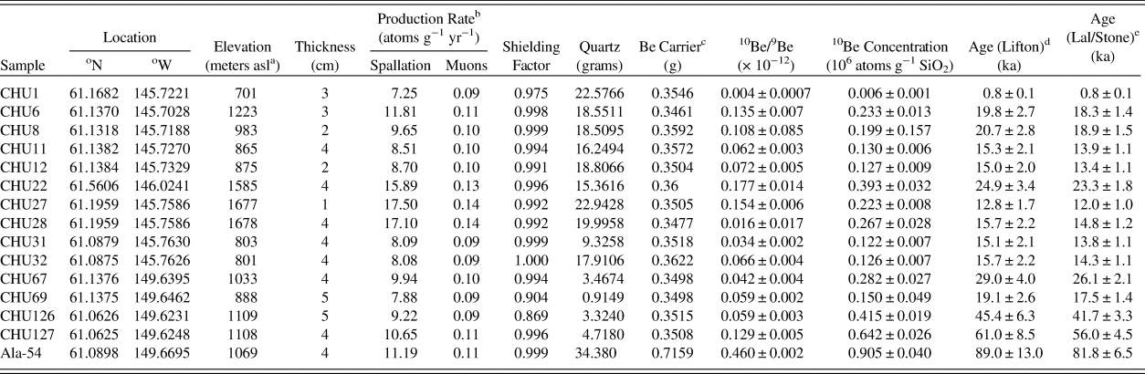
10Be TCN dating results.

a Above Sea Level (asl).
b The production rates are reported for the Lifton (Reference Lifton, Sato and Dunai2014) scaling factor.
c Carrier concentration = 1.414 ppm.
d LI of Marrero et al., Reference Marrero, Phillips, Borchers, Lifton, Aumer and Balco2015a.
e LM of Marrero et al., Reference Marrero, Phillips, Borchers, Lifton, Aumer and Balco2015a.
Constant local production rate based on Lifton (Reference Lifton, Sato and Dunai2014), Lal (Reference Lal1991), and Stone (Reference Stone2000).
AMS Standard = 07KNSTD.
rock density = 2.65 g/cm3.
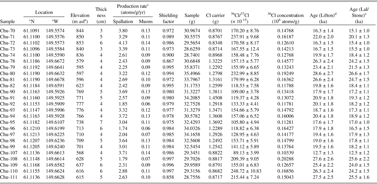
36Cl TCN dating results (all additional 36Cl chemical data is provided in Supplementary Table 1).

a asl, above sea level.
bConstant local production rate based on Lifton (Reference Lifton, Sato and Dunai2014), Lal (Reference Lal1991), and Stone (Reference Stone2000).
c The production rates are reported for the Lifton (Reference Lifton, Sato and Dunai2014) scaling factor.
d Lifton (LI) of Marrero et al., Reference Marrero, Phillips, Borchers, Lifton, Aumer and Balco2015a.
e Lal/Stone time-dependent (LM) of Marrero et al., Reference Marrero, Phillips, Borchers, Lifton, Aumer and Balco2015a.
Average of two blanks was 7.88 ± 0.98 × 10⁻¹⁵ (36Cl/37Cl).
Topographic shielding was calculated for every sample location using the site DEM and a Python-based ArcGIS tool that included the influence of the dip and aspect of the landscape (Li, Reference Li2018; Tables 2 and 3). The topographic shielding correction was applied to the ages when calculated with CRONUScalc. For the 36Cl samples, the production rate was 51.7 ± 4.9 atoms/g Ca/yr. The average uncertainty, including analytical and production rate/scaling model uncertainty, for individual 10Be exposure ages is 8.2% (Table 2) and 6.5% for the 36Cl ages (Table 3). For valid comparison of our ages with already published Alaskan chronologies, we recalculated the published ages using the same scaling model and production rate used in our study.
Statistical analysis of exposure ages
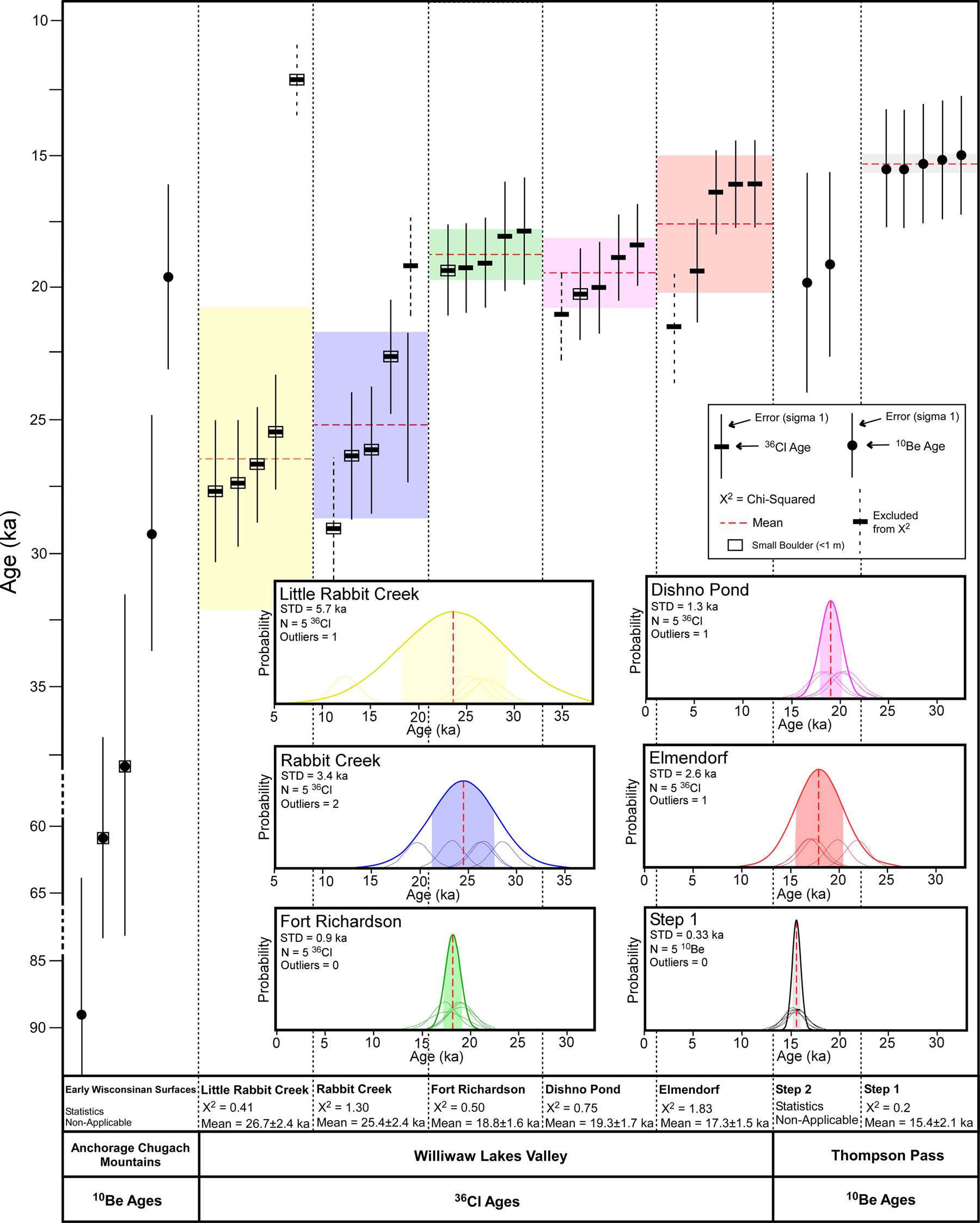
Exposure ages for each moraine were averaged and statistically analyzed for scatter and outliers. Each data cluster associated with an event with more than two ages was averaged using an unweighted mean (Fig. 7). In addition, we calculated the unweighted mean square weighted deviation (MSWD) statistic, otherwise known as the chi-squared (χ2) test, for each data set to determine the degree of scattering of the data sets using:

Distribution of measured 10Be and 36Cl ages for each moraine and mean square weighted deviation (MSWD) values for each data set. Probability plots for moraines and surfaces with a cluster of four or more ages. The 1-σ uncertainty is shown as the colored regions, and the mean is the dashed red line. Ages where the sampled boulder was less than 1 m in diameter are denoted by a box around the age symbol. STD, standard deviation. (For interpretation of the references to color in this figure legend, the reader is referred to the web version of this article.)

where N is the number of ages, ti is the exposure age, $\bar{t}$ is the average of ages, and σ is the age uncertainty (Fig. 7 in Balco, Reference Balco2010). The outliers identified using this method were eliminated from the feature data sets. The exposure age sets for Little Rabbit Creek, Rabbit Creek, Fort Richardson, Dishno Pond, and Elmendorf moraines in the Anchorage region and S1 at Thompson Pass were analyzed in this manner. The age range of each sample within the moraines was also graphically depicted as a probability plot to visualize the data's scatter and help identify outliers (Fig. 7). Subsequently, the outliers were removed from each feature data set if they were outside 1-σ of the data's mean on the probability plots.
Equilibrium-line altitude reconstructions
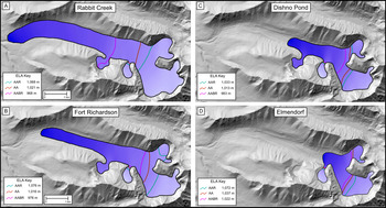
The geometries of the glacial limits for each of the late Pleistocene glaciations were used to calculate each glacier's former surface and were part of the modeling of the equilibrium-line altitude (ELA; Fig. 8). The results from field mapping of the Rabbit Creek, Fort Richardson, Dishno Pond, and Elmendorf moraines, including the locations of moraine termini and lateral moraines, glacial trimlines, and striations, chatter marks, and p-forms provided estimates of past glacial limits. The perimeters of the nine modern glaciers with closest proximity to the Williwaw Lakes valley were traced and used to model the current ELA for comparison. These include the Eagle River, Whiteout, Eklutna, and Hunter Creek glaciers and other subsidiary glaciers in the westernmost Chugach Mountains (Table 4).
(color online) Reconstruction of glacial extent and calculated equilibrium-line altitudes (ELAs; lines) using different methods for the late Pleistocene events in the Williwaw Lakes valley study area. The ice limits were constructed using the locations of end and lateral moraines, glacial trimlines, and former flow markers. The ELAs were calculated in ArcGIS, using the tools and methods of Pellitero et al. (Reference Pellitero, Rea, Spagnolo, Bakke, Hughes, Ivy-Ochs and Lukas2015).

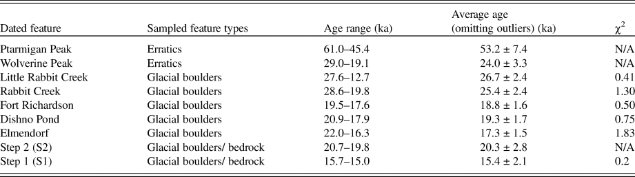
Summary of the results and statistical analysis for the TCN dating.

Former ELAs were calculated from reconstructed glacial limits in ArcGIS using the methods and tools from Pellitero et al. (Reference Pellitero, Rea, Spagnolo, Bakke, Hughes, Ivy-Ochs and Lukas2015). The contemporary ELA was calculated with the techniques of Pellitero et al. (Reference Pellitero, Rea, Spagnolo, Bakke, Hughes, Ivy-Ochs and Lukas2015) on the nearest modern glaciers (Fig. 1) and was used to compute the ELA depression (ΔELA) between the contemporary and Williwaw Lakes valley glacial limits (Table 4). The first step in the modeling involved reconstructing the former glacial area utilizing geomorphic evidence (Fig. 8). The ArcGIS Python-based toolbox from Pellitero et al. (Reference Pellitero, Rea, Spagnolo, Bakke, Hughes, Ivy-Ochs and Lukas2015) calculates the ELA using the area altitude (AA), accumulation area ratio (AAR), and area altitude balance ratio (AABR) methods. The AA method calculates the ELA by summing the products of the area and average altitude for each contour and dividing the sum by the total area of the glaciated basin (Osmaston, Reference Osmaston2005). The AAR method calculates the ELA by forming a ratio (0.5) of the accumulation area to the entire area of the glacier, where values of <0.5, 0.5–0.8, and >0.8 indicate negative mass balance, steady state, and positive mass balance, respectively (Osipov, Reference Osipov2004). The AABR method expands upon the AA method and calculates the ELA by iteratively calculating multiple former glacier mass balances for all possible ELAs (Osmaston, Reference Osmaston2005; Pellitero et al., Reference Pellitero, Rea, Spagnolo, Bakke, Hughes, Ivy-Ochs and Lukas2015).
RESULTS
Dating results
The ages of the sampled boulders and surfaces range from 61.0 to 19.1 ka for the previously interpreted early Wisconsinan surfaces, 28.6 to 16.3 ka for the moraines in Williwaw Lakes valley, and 20.7 to 15.0 ka on the surfaces in Thompson Pass (Tables 2 and 3). To serve as a test for regional inheritance in bedrock at Thompson Pass, a sample (CHU1) from polished bedrock located ~100 m downstream from the current ice limit of Worthington Glacier was dated and yielded an age of 0.8 ± 0.1 ka. This age shows that inheritance for the bedrock samples is likely not significant for the older samples, and we therefore made a correction for inheritance. We do not have 36Cl and 10Be ages from the same location, so we were not able to make direct comparison between nuclides. A simplified summary of the results for each sampled landform is shown in Table 5.
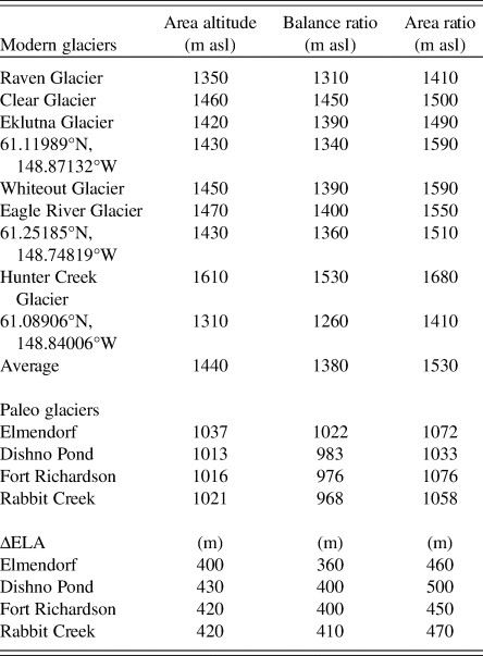
Summary of the equilibrium-line altitude (ELA) calculations in the Chugach Mountains.a

a The ELAs for the modern glaciers were calculated with the tools of Pellitero et al. (2015) to compare with the paleo ELAs from moraines. asl, above sea level.
We define the surfaces for the Ptarmigan and Wolverine Peaks using the oldest ages of the erratics. Statistical analysis of the moraines, except for the Elmendorf moraine, show that the older boulders are more likely representative of the moraine age. The Little Rabbit and Rabbit Creek moraines have ages ranging from 27.6 to 12.7 and 28.6 to 19.8 ka, respectively. The average ages (excluding outliers) for these moraines are 26.7 ± 2.4 and 25.4 ± 2.4 ka, highlighting that the older boulders are likely more representative of the age of deposition of the boulder as the ice retreated. The Fort Richardson and Dishno Pond moraines have average ages of 18.8 ± 1.6 and 19.3 ± 1.7 ka, with ranges of 19.5 to 17.6 and 20.9 to 17.9 ka, respectively. Again, the average ages highlight that the older boulders are likely representative of the age of deglaciation. The Elmendorf moraine has ages ranging from 22.0 to 16.3 ka, and the average age is 17.3 ± 1.5 ka (excluding one outlier). There are two overlapping ages for Step 2 that give an average age of 20.3 ± 2.8 ka. For Step 1, the bedrock and boulder ages are statistically identical, with an average age of 15.4 ± 2.1 ka, which provides confidence in this data set. An additional sample (CHU22) was collected from a glacially polished bedrock on top of a high ridge located ~40 km north of Thompson Pass and has an age of 24.9 ± 3.4 ka.
ELA results
The average modern ELAs for the glaciers closest to Williwaw Lakes valley are 1440 (AA), 1380 (AABR), and 1530 m asl (AAR) (Table 4). The ELA for the nearby Eklutna glacier is 1450 m asl (Dial et al., Reference Dial, Becker, Hope, Dial, Thomas, Alexandrovna, Golden and Shain2016; Sass et al., Reference Sass, Loso, Geck, Thoms and Mcgrath2017), which is similar to our results of 1390 m (AABR), 1420 m (AA) and 1490 m (AR). This, of course, assumes that the dynamics of the glaciers are the same since the Pleistocene. The calculated ELA of the AA method is closest to the measured result of Sass et al. (Reference Sass, Loso, Geck, Thoms and Mcgrath2017); therefore, all ELA comparisons in the text are based on the AA method (Pellitero et al., Reference Pellitero, Rea, Spagnolo, Bakke, Hughes, Ivy-Ochs and Lukas2015). The ΔELAs for the Williwaw Lakes moraines using the AA method are 420 m (Rabbit Creek), 420 m (Fort Richardson), 430 m (Dishno Pond), and 400 m (Elmendorf) (Fig. 8).
DISCUSSION
Our 10Be and 36Cl dating provide a new set of ages for the glacial landforms in the Chugach Mountains, enhancing previous radiocarbon dating and extending the glacial chronology into the early Wisconsinan beyond the range of radiocarbon methods. Based on the spread of ages and the fact that it was challenging to find optimal sampled glacial boulders near the Williwaw Lakes valley region that were not prone to the possibility of surface modification, we highlight that the ages for the Rabbit Creek moraines are not well defined. A correlation of small sampled boulders (<1 m in diameter) with age distribution indicates little negative influence to scatter, yet the errors of these ages are considerably high (Fig. 7). However, considering these factors, these ages warrant being reported to provide the best estimates for these landforms and surfaces.
One of the ages on Ptarmigan Peak (61.0 ± 8.5 ka) and the age on Flattop Mountain (89.0 ± 13.0 ka) roughly define the timing for the lLGM during the early Wisconsinan in the Chugach Mountains. These results are comparable to the early Wisconsinan ages recorded in the Ahklun Mountains, which show a maximum age of ~70 ka (Kaufman et al., Reference Kaufman, Manley, Forman and Layer2001), a minimum age of ~39 ka (Manley et al., Reference Manley, Kaufman and Briner2001), and a range of 56–53 ka (Briner et al., Reference Briner, Swanson and Caffee2001). The second age on Ptarmigan Peak is 45.4 ± 6.3 ka and is probably younger, because the sampled glacial boulder may have moved, been exhumed, or weathered after deposition. Along these lines, the ages of granitic boulders on Wolverine Mountain of 29.0 ± 4.0 and 19.1 ± 2.6 ka also imply that the slopes have been unstable since the glacier deposited the boulders. The morphology of the Wolverine Mountain step is steeply sloped and located ~100–200 m below the elevations of Ptarmigan Peak and Flattop Mountain, suggesting that this surface may have been influenced by either more recent glacial advances or erosion.
The presence of granitic boulders and clasts on these likely early Wisconsinan surfaces indicates that glaciers may have transported debris ~80 km south to the Chugach Mountains from the Talkeetna Mountains that are the nearest granitic rock outcrops are present (Fig. 1). Only an exceptionally large glacial advance(s) could have transported the granitic rocks this distance and deposited them over 1000 m on these mountainous uplands. Based on the Wolman's pebble analysis, the comparison between the granitic clasts (well rounded) and the Chugach Group clasts (angular) implies that the granitic source material was transported and eventually mixed with the local material (see clast data in Supplementary Table 1). The late Wisconsinan moraines at lower elevations contained no granitic clasts and were instead composed entirely of sandstone, siltstone, and metasediments present in the Chugach Mountains. This suggests that the glacial advances may have been less extensive in the late Wisconsinan than during the older events.
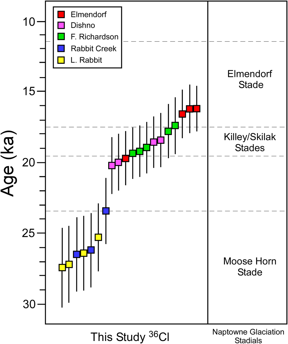
The 36Cl moraine ages in Williwaw Lakes valley range from 28.6 ± 2.7 to 16.3 ± 1.4 ka (Figs. 3 and 7), and as expected, the ages of the moraines are oldest at the mouth of the valley and become successively younger upvalley. These ages follow the general pattern of deglaciation observed across Alaska since the gLGM as described by Briner and Kaufman (Reference Briner and Kaufman2008). The ages show that the moraines in the Williwaw Lakes valley broadly correlate with the Naptowne glaciation on the Kenai Peninsula (Karlstrom, Reference Karlstrom1964; Reger et al., Reference Reger, Sturmann, Berg and Burns2007; Fig. 9). The Little Rabbit Creek (26.7 ± 2.4 ka) and Rabbit Creek (25.4 ± 2.4 ka) moraines are both coeval with the broad age range of 32–25 ka defined for the Moose Horn stade (Reger et al., Reference Reger, Sturmann, Berg and Burns2007; Fig. 9). This implies two distinct yet close in time (statistically their ages are the same) glacial advances during this stade in the Anchorage area. Schmoll et al. (Reference Schmoll, Yehle and Updike1999) suggested that the Little Rabbit Creek moraine formed during the early Wisconsinan, yet our new ages indicate that it is much younger, with a similar age to the Rabbit Creek event. Both moraines are possibly related to the same deglaciation and simply record variations in retreat rate and moraine deposition. These interpretations of the Rabbit Creek moraines are loosely based on a scattered data set of ages collected from small glacial boulders.
(color online) A correlation of our new 36Cl exposure ages with the recalculated local chronology of the Naptowne glaciation of Karlstrom (Reference Karlstrom1964). The Elmendorf stade interval is defined by the results of the work from Kopczynski et al. (Reference Kopczynski, Kelley, Lowell, Evenson and Applegate2017), and the remaining stadial intervals are sourced from Reger et al. (Reference Reger, Sturmann, Berg and Burns2007). The age intervals for the Kiley and Skilak stades overlapped significantly; therefore, they are lumped together in this diagram.

The Fort Richardson (18.8 ± 1.6 ka) and the Dishno Pond (19.3 ± 1.7 ka) moraines have statistically overlapping ages, and the Fort Richardson moraine is morphostratigraphically bracketed between Rabbit Creek and Dishno Pond; therefore, the age must be between 25.4 ± 2.4 and 19.3 ± 1.7 ka. Although the Fort Richardson moraine ages are tightly clustered, they disagree with the morphostratigraphic relationship, which places the moraine between the Dishno Pond and Rabbit Creek moraines. The ages of these two moraine sets are within error of each other (~1.5 ka); therefore, it is possible that there was rapid retreat from the Fort Richardson to Dishno Pond events and that the details are obscured in the noise of sample variety.
The ages of the Elmendorf moraine (17.3 ± 1.5 ka) are similar to those for the original Elmendorf stade age range of ~16.8–14.2 ka based on Karlstrom radiocarbon dating (Reger et al., Reference Reger, Sturmann, Berg and Burns2007) and correlate well with the recalibrated ages at ~11.5–17.5 from the recent work of Kopczynski et al. (2017; Fig. 9). Our results mimic the oldest ages from Kopczynski et al. (Reference Kopczynski, Kelley, Lowell, Evenson and Applegate2017), correlating with the beginning of deglaciation and retreat of the Matanuska-Knik glacier lobe.
The 10Be exposure ages of the glacial boulders and glacially polished bedrock in Thompson Pass indicate that either glaciers retreated at least twice during the late Wisconsinan glaciation at ~20.3 ± 2.8 and ~15.4 ± 2.1 ka (Fig. 6) or progressively retreated in one event from high to low elevations within these periods. The highest glacially polished step in Thompson Pass (S3) at ~1300 m asl was not dated, but the chronostratigraphy suggests more extensive glacial activity before ~20.3 ± 2.8 ka. The single age of 12.8 ± 1.7 ka on a polished bedrock ridge above an actively glaciated part of the pass suggests that a glacier advanced during the Younger Dryas, but more data are needed to quantify the extent of the possible Younger Dryas advance. The single age from sample CHU22, located ~40 km north of Thompson Pass with an age of 24.9 ± 3.4 ka and at an elevation of 1585 m asl, roughly correlates with the S3 and is older than the S2 step.
The ΔELAs in Williwaw Lakes valley ranged from 430 to 400 m for several advances during the late Wisconsinan. These ΔELAs are consistent with the lower-limit ΔELA values of ~300–600 m of Briner and Kaufman (Reference Briner and Kaufman2000) in western Alaska and ΔELA of ~200–700 m of Balascio et al. (Reference Balascio, Kaufman and Manley2005) in the Brooks Range. The modern ELA for western Alaska is 900 m (Briner and Kaufman, Reference Briner and Kaufman2000) and the ELA for the Brooks Range is 2000 m (Balascio et al, Reference Balascio, Kaufman and Manley2005). Balascio et al. (Reference Balascio, Kaufman and Manley2005) concluded that the Alaskan ΔELAs were ~600 m less than the global average (~1000 m) for the gLGM (Broecker and Denton, Reference Broecker and Denton1990). During the gLGM, sea level was ~125 m lower (Fairbanks, Reference Fairbanks1989), which would have created greater continentality and would have reduced precipitation in Alaska (Broecker, Reference Broecker1997). We favor the possibility of reduced precipitation in the late Wisconsinan, because our ΔELA values are at the low end (~600 m) of the estimated range for Alaska during the lLGM (Balascio et al., Reference Balascio, Kaufman and Manley2005). The western Chugach Mountains possibly experienced either a greater drop in precipitation during the lLGM or the Alaska interior experienced a smaller rise in precipitation since the lLGM. The regional variations in the timing of late Wisconsinan glacial advances in mountain ranges is possibly related to changes in climate, previously associated with orographically controlled precipitation gradients and atmospheric circulation, plus changes in the dominant regional pressure systems due to the advance and retreat of Laurentide Ice Sheet (Otto-Bliesner et al., Reference Otto-Bliesner, Brady, Clauzet, Tomas, Levis and Kothavala2006; Briner and Kaufman, Reference Briner and Kaufman2008; Pendleton et al., Reference Pendleton, Ceperley, Briner, Kaufman and Zimmerman2015; Tulenko et al., Reference Tulenko, Lofverstrom and Briner2020). While the high modern precipitation in the coastal mountain belt keeps modern ELA values relatively low, the rest of Alaska may have only experienced a minor increase in precipitation, such that ELA climbed much higher there as temperatures warmed following lLGM.
An alternative explanation for the smaller ΔELA in the western Chugach Mountains relative to the rest of Alaska and Alaska relative to the global trend is that local and regional temperatures experienced less cooling during the gLGM (Porter et al., Reference Porter, Pierce, Hamilton and Porter1983). For example, the Chugach Mountains may have experienced local changes in coastal atmospheric circulation that depressed the cooling effect that occurred in the Alaskan interior. Assuming a mean alpine environmental lapse rate of −5.7°C/km (Rolland, Reference Rolland2003; Kirchner et al., Reference Kirchner, Faus Kessler, Jakobi, Leuchner, Ries, Scheel and Suppan2013), the ΔELA ranges of the events in the Williwaw Lakes valley represent a temperature decrease of 2.1–2.3°C. This analysis provides us with a potential maximum temperature depression for the gLGM in the Chugach Mountains. For regional comparisons against global values, the average temperature depressions for other glaciers in South America during the gLGM were 5–6.4°C (Porter, Reference Porter2000), 8.8–11°C in the central Andes (Stansell et al., Reference Stansell, Polissar and Abbott2007), 1.9–3.0°C throughout the Himalayas (Heyman, Reference Heyman2014), 5.5–8.0°C in the Uinta Mountains (Munroe and Mickelson, Reference Munroe and Mickelson2002), and 5–7°C for New Zealand (McCarthy et al., Reference McCarthy, Mackintosh, Rieser and Fink2008). Except for some of the Himalayan results, the comparatively low-temperature depression in the Chugach Mountains may imply that the climate cooled less in Alaska than in many other regions throughout the globe during the gLGM and, likewise, that the coastal mountains may have cooled less than the Alaska interior.
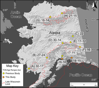
Our new ages provide the first cosmogenic glacial chronology for the Chugach Mountains, which can be used to establish chronologies in adjacent regions throughout Prince William Sound. Comparison of the Chugach glacial chronology with the timing of glaciation in adjacent mountain ranges throughout Alaska depicts a broad pattern of uniform deglaciation in Alaskan ranges, with slightly younger ages toward the southeast and the main body of the Cordilleran Ice Sheet (Fig. 10). These new ages help fill the gap in the regional glacial chronology showing later deglaciation in south-central Alaska compared with the rest of the state. Specifically, the pattern of deglaciation followed the high topography and mountain ranges in Alaska, progressively moved from west to east, and was predominantly controlled by precipitation gradients. Glaciation in the Cook Inlet and the surrounding mountains may behave asynchronously in the future as compared with global patterns, as it did during the lLGM and gLGM.
Exposure age ranges for the late Wisconsin glaciations in Alaska. The numbers in the rectangles are ages in ka. The yellow points represent previous studies, and the orange locations are from the current study. The base map is modified from Riehle (Reference Riehle2011). The late Wisconsinan limits are from Briner and Kaufman (Reference Briner and Kaufman2008). A, Ahklun Mountains (Briner et al. Reference Briner, Swanson and Caffee2001); B, Lime Hills (Briner et al. Reference Briner, Kaufman, Manley, Finkel and Caffee2005); C, Yukon Tana Upland (Briner et al. Reference Briner, Kaufman, Manley, Finkel and Caffee2005); D, Central Alaska Range (Dortch et al. Reference Dortch, Owen, Caffee, Li and Lowell2010b); E, Denali Fault (Matmon et al. Reference Matmon, Schwartz, Haeussler, Finkel, Lienkaemper, Stenner and Dawson2006); F, Fish Lake valley (Young et al. Reference Young, Briner and Kaufman2009); G, Central Brooks Range (Badding et al. Reference Badding, Briner and Kaufman2013); H, Brooks Range (Pendleton et al. Reference Pendleton, Ceperley, Briner, Kaufman and Zimmerman2015); I, Knik Arm (Kopczynski et al. Reference Kopczynski, Kelley, Lowell, Evenson and Applegate2017). (For interpretation of the references to color in this figure legend, the reader is referred to the web version of this article.)

CONCLUSION
Geomorphic mapping, 10Be and 36Cl exposure age dating, and ELA reconstructions help define the timing of glaciation and climatic condition since the lLGM in the western Chugach Mountains of Alaska. The presence of old erratics and rounded granitic clasts in the early Wisconsinan moraines indicates an origin of either the Talkeetna Mountains or Alaska Range to the north and supports the current model that the lLGM glaciations were more extensive than the gLGM events, because the boulders were transported and deposited ~1000 m above the contemporary valley floor. Exposure ages in Williwaw Lakes valley establish a chronology for moraines that roughly correspond to the stades of the Naptowne chronology on the Kenai Peninsula to the south and support the existing detailed results of the Matanuska-Knik glacier lobe. The Little Rabbit (26.7 ± 2.4 ka) and Rabbit Creek (25.4 ± 2.4 ka) moraines had the greatest age uncertainty, yet still roughly correlated with the Moosehorn stade. The Fort Richardson (18.8 ± 1.6 ka) and Dishno Pond (19.3 ± 1.7 ka) moraine ages are close to one another and may correlate with the Killey and Skilak stades. The Elmendorf moraine ages cluster well around 16.4 ka and correspond very well with the prior work and dating on this glaciation (Table 1). Ages from Thompson Pass exhibit two age clusters at 20.3 ± 2.8 and 15.4 ± 2.1 ka, which correspond to the S1 step (at ~800 m asl) and S2 step (at ~1200 m asl), respectively. Digital and field-based geomorphic mapping facilitated the reconstruction of the past ice extent in Williwaw Lakes valley and the calculation of ELAs during the late Wisconsinan. The ΔELAs range from 430 to 400 m, which corresponds with the low average of ΔELAs from other mountain ranges in Alaska, implying that the climate may have been drier and warmer than the global average during the gLGM. The ages from this study complement the overall scenario in Alaska, where the Cordilleran Ice Sheet has progressively retreated from west to east and the deglaciation has been influenced by the high topography and mountain ranges and precipitation gradients that control both the style and magnitude of glaciation.
ACKNOWLEDGMENTS
We thank two anonymous reviewers, associate editor Yeong Bae Seong, and senior editor Nicholas Lancaster for their very constructive and positive reviews, which greatly helped improve our contribution. We also thank Michelle Fame for helpful discussions, Zachary Kirkpatrick for assistance with fieldwork, and Sarah Hammer with sample preparation and processing. Additionally, we thank Robert K. Denton Jr for providing support as a technical reviewer. Support was provided by the National Science Foundation grant EAR-1123688/1123643 and a seed grant from the Purdue University PRIME Lab.
SUPPLEMENTARY MATERIAL
The supplementary material for this article can be found at https://doi.org/10.1017/qua.2020.106