



1 Introduction
The compressible (flat plate) turbulent boundary layer (CTBL) is a paradigm flow of major engineering significance. It serves as a benchmark for a large variety of technological flows, such as high-speed aircraft, combustion ramjet engines, gas turbine blades, rocket motor nozzles, etc. (Bradshaw Reference Bradshaw1977; Smits & Dussauge Reference Smits and Dussauge2006; Gatski & Bonnet Reference Gatski and Bonnet2013). Its simple geometry makes CTBL ideal for fundamental studies aiming to explain the physics of compressible turbulence. Important questions concern the Reynolds number (
 $Re$
) and Mach number (
 $Ma$
) scaling of the mean profiles of velocity and temperature, along the streamwise direction (i.e.
 $Re$
effect) and as a function of the incoming velocity (i.e.
 $Ma$
effect). Two basic scaling laws feature in the classical approach: the celebrated log law characterizing
 $Re$
similarity (Prandtl Reference Prandtl1925; von Karman Reference von Karman1930), and the Morkovin scaling characterizing
 $Ma$
effects (Morkovin Reference Morkovin and Favre1962); the latter is formulated in the so-called van Driest transformation (van Driest Reference van Driest1951). However, recent direct numerical simulations (DNS) show that the van Driest transformed mean velocity is only approximately invariant in the log layer (Huang, Coleman & Bradshaw Reference Huang, Coleman and Bradshaw1995; Duan, Beekman & Martin Reference Duan, Beekman and Martin2010; Hadjadj et al.
Reference Hadjadj, Ben-Nasr, Shadloo and Chaudhuri2015; Shadloo, Hadjadj & Hussain Reference Shadloo, Hadjadj and Hussain2015), with significant data scatter in the near-wall region in the case of strong heat flux (Brun et al.
Reference Brun, Boiarciuc, Haberkorn and Comte2008; Duan et al.
Reference Duan, Beekman and Martin2010; Trettel & Larsson Reference Trettel and Larsson2016). To predict CTBLs, Computational Fluid Dynamics (CFD) applications integrate the Reynolds averaged Navier–Stokes (RANS) equation with models involving typically many adjustable parameters lacking sufficient physical/theoretical understanding (Huang, Bradshaw & Coakley Reference Huang, Bradshaw and Coakley1994; Roy & Blottner Reference Roy and Blottner2006; Spalart Reference Spalart2006). Existing closure models for CTBL primarily emulate models established and calibrated for incompressible flows, and typically employ the Morkovin hypothesis (Morkovin Reference Morkovin and Favre1962). As reviewed in Wu et al. (Reference Wu, Bi, Hussain and She2017), the van Driest wall damping function (van Driest Reference van Driest1956) extending the profile from the log region to the wall yields only a moderately accurate mean velocity profile (MVP). In addition, the eddy-viscosity-based closure for the energy equation is inadequate (as shown herein). Therefore, despite efforts over several decades, accurate prediction of the mean quantities across the entire boundary layer remains unsatisfactory (Dong & Zhou Reference Dong and Zhou2010; Rumsey Reference Rumsey2010; Dong & Li Reference Dong and Li2011). This is particularly challenging in supersonic and hypersonic regimes (Wilcox Reference Wilcox2006; Slotnick et al.
Reference Slotnick, Khodadoust, Alonso, Darmofal, Gropp, Lurie and Mavriplis2014), presumably owing to the absence of an analytic understanding of the
 $Ma$
-invariant structure.
The present work aims to resolve the above issues from a newly developed symmetry-based approach to quantifying wall turbulence (She, Chen & Hussain Reference She, Chen and Hussain2017; Chen, Hussain & She Reference Chen, Hussain and She2018). The theory, called structural ensemble dynamics (SED) (She et al.
Reference She, Chen, Wu and Hussain2010, Reference She, Chen and Hussain2017), expresses the essential similarity property of wall turbulence in terms of a multi-layer analytic form of a stress length (SL) function,
 $\ell _{12}$
, quantifying turbulence eddy scales (hereafter, we refer to the derived algebraic model as the SED-SL model). The multi-layer form is arguably universal, since it incorporates the (dilation) symmetry constraint due to the presence of the wall, which has successfully yielded unified description of various mean profiles in a variety of wall flows – for both channel/pipe (internal flow) and TBL (external flow) (She et al.
Reference She, Chen and Hussain2017), including both mean velocity (Chen & She Reference Chen and She2016; Chen, Hussain & She Reference Chen, Hussain and She2016a
) and turbulence intensity profiles (Chen et al.
Reference Chen, Wei, Hussain and She2016c
, Reference Chen, Hussain and She2018), and also for smooth as well as rough wall (She et al.
Reference She, Wu, Chen and Hussain2012), etc. The objective of the present work is to assert the validity of the multi-layer description of
 $\ell _{12}$
over a range of
 $Ma$
values, based on our previous study (Zhang et al.
Reference Zhang, Bi, Hussain, Li and She2012). As shown below, the multi-layer structure (with universal constants such as layer thicknesses and scaling exponents) can yield decidedly improved predictions.
Compared to existing models, three features of the present SED-SL model are noteworthy. First, it is straightforwardly developed from the theory in She et al. (Reference She, Chen and Hussain2017), which describes the entire domain of the turbulent boundary layer with a smooth transition from the inner to outer flow regions. This is in contrast to the Baldwin–Lomax (BL) model for which an artificial matching location
 $y_{c}$
is needed. Second, the present model contains only physical parameters defining the multi-layer structure; for current CTBLs, these parameters are invariant, so as to possess a
 $Ma$
-invariant scaling. Third, a notable improvement of the prediction accuracy is achieved for all mean profiles, including velocity and temperature. These features validate the dilation invariance of the stress length function and also the generalized Reynolds analogy in CTBL. To become a mature CFD model, the analytic form proposed in this paper needs to be tested in other benchmark flows, such as flow with wall curvature, pressure gradient, transition etc. (for more discussion, see § 5).
The paper is organized as follows. Section 2 describes our model, computational set-up, the DNS dataset and other models for benchmarking purposes. Section 3 describes the results of computation, which validate our predictions for different
 $Ma$
values and
 $Re$
values. Section 4 is devoted to discussion and interpretation. Section 5 is the conclusion.
2 Theory
We describe a statistically stationary CTBL by the averaged two-dimensional compressible Navier–Stokes equations:
 $$\begin{eqnarray}\displaystyle & \displaystyle {\displaystyle \frac{\unicode[STIX]{x2202}\overline{\unicode[STIX]{x1D70C}u}}{\unicode[STIX]{x2202}x}}+{\displaystyle \frac{\unicode[STIX]{x2202}\overline{\unicode[STIX]{x1D70C}v}}{\unicode[STIX]{x2202}y}}=0; & \displaystyle\end{eqnarray}$$
 $$\begin{eqnarray}\displaystyle & \displaystyle {\displaystyle \frac{\unicode[STIX]{x2202}\bar{\unicode[STIX]{x1D70C}}\tilde{u} }{\unicode[STIX]{x2202}x}}+{\displaystyle \frac{\unicode[STIX]{x2202}\bar{\unicode[STIX]{x1D70C}}\tilde{u} \tilde{v}}{\unicode[STIX]{x2202}y}}={\displaystyle \frac{\unicode[STIX]{x2202}}{\unicode[STIX]{x2202}y}}(\bar{\unicode[STIX]{x1D70F}}_{12}-\overline{\unicode[STIX]{x1D70C}u^{\prime \prime }v^{\prime \prime }}); & \displaystyle\end{eqnarray}$$
 $$\begin{eqnarray}\displaystyle & \displaystyle {\displaystyle \frac{\unicode[STIX]{x2202}\bar{\unicode[STIX]{x1D70C}}\tilde{v}}{\unicode[STIX]{x2202}x}}+{\displaystyle \frac{\unicode[STIX]{x2202}\bar{\unicode[STIX]{x1D70C}}\tilde{v}\tilde{v}}{\unicode[STIX]{x2202}y}}={\displaystyle \frac{\unicode[STIX]{x2202}}{\unicode[STIX]{x2202}x}}(\bar{\unicode[STIX]{x1D70F}}_{12}-\overline{\unicode[STIX]{x1D70C}u^{\prime \prime }v^{\prime \prime }}). & \displaystyle\end{eqnarray}$$
 $$\begin{eqnarray}\displaystyle {\displaystyle \frac{\unicode[STIX]{x2202}}{\unicode[STIX]{x2202}x}}\left(\bar{\unicode[STIX]{x1D70C}}\tilde{e}\tilde{u} +\tilde{p}\tilde{u} \right)+{\displaystyle \frac{\unicode[STIX]{x2202}}{\unicode[STIX]{x2202}y}}\left(\bar{\unicode[STIX]{x1D70C}}\tilde{e}\tilde{v}+\tilde{p}\tilde{v}\right) & = & \displaystyle {\displaystyle \frac{\unicode[STIX]{x2202}}{\unicode[STIX]{x2202}x}}\left(\tilde{v}\left(\bar{\unicode[STIX]{x1D70F}}_{12}-\overline{\unicode[STIX]{x1D70C}u^{\prime \prime }v^{\prime \prime }}\right)+C_{p}{\displaystyle \frac{\unicode[STIX]{x1D707}}{\mathit{Pr}}}{\displaystyle \frac{\unicode[STIX]{x2202}\tilde{T}}{\unicode[STIX]{x2202}x}}-C_{p}\overline{\unicode[STIX]{x1D70C}u^{\prime \prime }T}\right)\nonumber\\ \displaystyle & & \displaystyle +\,{\displaystyle \frac{\unicode[STIX]{x2202}}{\unicode[STIX]{x2202}y}}\left(\tilde{u} \left(\bar{\unicode[STIX]{x1D70F}}_{12}-\overline{\unicode[STIX]{x1D70C}u^{\prime \prime }v^{\prime \prime }}\right)+C_{p}{\displaystyle \frac{\unicode[STIX]{x1D707}}{\mathit{Pr}}}{\displaystyle \frac{\unicode[STIX]{x2202}\tilde{T}}{\unicode[STIX]{x2202}y}}-C_{p}\overline{\unicode[STIX]{x1D70C}v^{\prime \prime }T}\right),\nonumber\\ \displaystyle & & \displaystyle\end{eqnarray}$$
where
 $\tilde{f}=\overline{\unicode[STIX]{x1D70C}f}/\overline{\unicode[STIX]{x1D70C}}$
denotes Favre averaging (FA) (with its fluctuation denoted by
 $f^{\prime \prime }=f-\tilde{f}$
), and overbar indicates time and space average (Reynolds averaging). In (2.1)–(2.4), all symbols are classically defined:
 $\unicode[STIX]{x1D70C}$
the density,
 $u$
and
 $v$
the streamwise and normal velocities,
 $e=C_{v}T+k$
with
 $C_{v}$
the specific heat at constant volume,
 $T$
the static temperature and
 $k$
the kinetic energy of the flow,
 $\unicode[STIX]{x1D707}$
the dynamic viscosity,
 $Pr$
the Prandtl number,
 $C_{p}$
the specific heat at the constant pressure,
 $p=\unicode[STIX]{x1D70C}RT$
is the static pressure (
 $R$
is the gas constant). The stress tensor is given by
 $\unicode[STIX]{x1D70F}_{12}=\unicode[STIX]{x1D707}(\unicode[STIX]{x2202}u/\unicode[STIX]{x2202}y+\unicode[STIX]{x2202}v/\unicode[STIX]{x2202}x)$
, with
 $\unicode[STIX]{x1D707}$
the dynamic viscosity. Equations (2.2) and (2.3) are unclosed, because of the unknown Reynolds shear stress (
 $-\overline{\unicode[STIX]{x1D70C}u^{\prime \prime }v^{\prime \prime }}$
) in (2.2)–(2.3) and several correlation terms in (2.4). We will theoretically close the system via the proposed symmetry approach. In this paper, we compare our theoretical description to a full three-dimensional DNS of CTBL with
 $\mathit{Pr}=0.7$
. In the DNS,
 $\unicode[STIX]{x1D707}$
is assumed to obey Sutherland’s law as usual:
 $\unicode[STIX]{x1D707}/\unicode[STIX]{x1D707}_{\infty }=(1\text{ + }T_{s}/T_{\infty })/(T/T_{\infty }+T_{s}/T_{\infty })(T/T_{\infty })^{3/2}$
, where
 $T_{S}=110.4$
(K) and subscript
 $\infty$
indicates the free-stream property.
To unify the notation, it is useful to express the Reynolds averaged (RA) variables in (2.1)–(2.4) in terms of the FA variables. For example, the mean pressure is expressed by
 $\overline{p}\approx R\overline{\unicode[STIX]{x1D70C}}\tilde{T}$
. On the other hand, for the RA shear stress
 $\bar{\unicode[STIX]{x1D70F}}_{12}$
, it can be rewritten approximately (Wu Reference Wu2016) as
 $$\begin{eqnarray}\bar{\unicode[STIX]{x1D70F}}_{12}=\bar{\unicode[STIX]{x1D707}}\left({\displaystyle \frac{\unicode[STIX]{x2202}\tilde{u} }{\unicode[STIX]{x2202}y}}+{\displaystyle \frac{\unicode[STIX]{x2202}\tilde{v}}{\unicode[STIX]{x2202}x}}\right),\end{eqnarray}$$
where the dynamic viscosity
 $\overline{\unicode[STIX]{x1D707}}$
satisfies the Sutherland formula as a function of
 $\tilde{T}$
. The energy equation will not be treated here, since we employ a generalized Reynolds analogy (GRA) approximation (see below). Then, the only term in (2.2)–(2.3) to be modelled is the Reynolds stress which is described by the stress length function below.
2.1 A multi-layer stress length function
In She et al. (Reference She, Chen and Hussain2017), it is assumed that a stress length,
 $\ell _{12}$
defined from the Reynolds shear stress (
 $-\overline{\unicode[STIX]{x1D70C}u^{\prime \prime }v^{\prime \prime }}$
), possesses the dilation symmetry, so that its analytic form can be readily obtained, specifying a physically sound multi-layer structure for canonical wall turbulence. Taking the incompressible TBL as an example (for which the Reynolds averaging is identical to the Favre averaging), the stress length
 $\ell _{12}$
is defined by:
 $$\begin{eqnarray}-\overline{u^{\prime }v^{\prime }}=\ell _{12}^{2}(\unicode[STIX]{x2202}_{y}U)^{2}\quad \text{or}\quad \ell _{12}=\sqrt{-\overline{u^{\prime }v^{\prime }}}/\unicode[STIX]{x2202}_{y}U,\end{eqnarray}$$
where
 $U=\overline{u}$
is the mean velocity. Note that the boundary layer approximation is adopted so that
 $\unicode[STIX]{x2202}_{y}U\gg \unicode[STIX]{x2202}_{x}V$
and
 $\unicode[STIX]{x2202}_{x}V$
is omitted. Also, equation (2.6) coincides with Prandtl’s mixing length Prandtl (Reference Prandtl1925), but we uncover its role of preserving the dilation symmetry and its physical interpretation of length scale of eddy (at wall distance
 $y$
) responsible for the transport of momentum normal to the wall.
The stress length
 $\ell _{12}$
is shown (She et al.
Reference She, Chen and Hussain2017) to display the following multi-layer structure:
 $$\begin{eqnarray}\displaystyle \ell _{12}^{+} & = & \displaystyle \ell _{12}^{+In}\ell _{12}^{+Outer}/(\unicode[STIX]{x1D705}y^{+}),\end{eqnarray}$$
where the inner (wall) function
 $\ell ^{+In}$
is
 $$\begin{eqnarray}\displaystyle \ell _{12}^{+In}=\ell _{0}(y^{+}/y_{s}^{+})^{+3/2}[1+(y^{+}/y_{s}^{+})^{4}]^{1/8}[1+(y^{+}/y_{b}^{+})^{4}]^{-1/4}, & & \displaystyle\end{eqnarray}$$
and the outer (wake) function is
 $$\begin{eqnarray}\ell _{12}^{+Outer}=\unicode[STIX]{x1D705}\unicode[STIX]{x1D6FF}^{+}(1-r^{4})/4.\end{eqnarray}$$
Here, superscript
 $+$
denotes the viscous wall units normalization;
 $y^{+}=yu_{\unicode[STIX]{x1D70F}}/\unicode[STIX]{x1D708}_{w}$
is the distance to the wall, and
 $r=1-y/\unicode[STIX]{x1D6FF}$
is the distance away from the boundary layer edge;
 $\ell ^{+}=\ell u_{\unicode[STIX]{x1D70F}}/\unicode[STIX]{x1D708}_{w}$
with
 $\unicode[STIX]{x1D708}_{w}$
the kinematic viscosity at the wall; the outer flow variable
 $r$
is restricted to
 $y\leqslant 2\unicode[STIX]{x1D6FF}$
so that
 $|r|\leqslant 1$
, and
 $\ell ^{+outer}$
is positive.
The derivation of (2.7)–(2.9) from a dilation symmetry assumption is given in detail in She et al. (Reference She, Chen and Hussain2017), which is summarized as follows. First, by assuming a constant dilation invariant of the stress length (which corresponds to ansatz one in She et al. (Reference She, Chen and Hussain2017)), we obtain
 $\ell _{12}\propto y^{3/2}$
in the viscous sublayer and
 $\ell _{12}\propto y^{2}$
in the buffer layer; both scaling exponents (i.e.
 $3/2$
and 2) can be analytically derived: introduce an eddy-dissipation length,
 $\ell _{\unicode[STIX]{x1D708}}=\unicode[STIX]{x1D708}_{T}^{3/4}/\unicode[STIX]{x1D700}^{1/4}$
(
 $\unicode[STIX]{x1D708}_{T}^{}=-\langle u^{\prime }v^{\prime }\rangle /\unicode[STIX]{x2202}_{y^{+}}U^{+}$
is eddy viscosity, and
 $\unicode[STIX]{x1D700}$
is the sum of viscous dissipation and diffusion), then,
 $\ell _{12}=\ell _{\unicode[STIX]{x1D708}}\unicode[STIX]{x1D6E9}^{1/4}$
(where
 $\unicode[STIX]{x1D6E9}\equiv -\langle u^{\prime }v^{\prime }\rangle \unicode[STIX]{x2202}_{y^{+}}U^{+}/\unicode[STIX]{x1D700}$
is the production–dissipation ratio). For small
 $y^{+}\rightarrow 0$
,
 $-\overline{u^{\prime }v^{\prime }}\propto y^{3}$
and a constant mean shear in the viscous sublayer, while
 $\ell _{\unicode[STIX]{x1D708}}=\unicode[STIX]{x1D708}_{T}^{3/4}/\unicode[STIX]{x1D700}^{1/4}\propto y^{2}$
and a constant dissipation–production ratio
 $\unicode[STIX]{x1D6E9}$
in the buffer layer. Then, applying ansatz three in She et al. (Reference She, Chen and Hussain2017), we obtain an analytic expression connecting the viscous sublayer and buffer layer scalings. Furthermore, for obtaining the bulk scaling with respect to the variable
 $r$
, we assume the constant dilation invariant for the derivative of the stress length (ansatz two in She et al. (Reference She, Chen and Hussain2017)), which yields a defect power law of
 $\ell \propto (1-r^{4})/4$
(i.e. (2.10)), where the exponent 4 for the planar geometry is derived in Chen et al. (Reference Chen, Hussain and She2016a
) with a variational argument which additionally predicts an exponent 5 for the circular geometry (e.g. for pipe flow). Finally, using the multiplicative rule for the scaling transition formula, composite expressions valid for the inner flow (i.e. (2.8)) and the entire flow (i.e. (2.7)) are obtained.
She et al. (Reference She, Chen and Hussain2017) assert that
 $y_{s}^{+}=9.7$
and
 $y_{b}^{+}=41$
, and the former seems to be universal while the latter exhibits moderate
 $Re$
-dependence. More recently, we theoretically obtain
 $y_{buf}^{+}=43.8$
for asymptotically large
 $Re$
values (not discussed here). Furthermore, as explained in She et al. (Reference She, Chen and Hussain2017), a
 $4\,\%$
variation of
 $y_{buf}^{+}$
would yield a
 $2\,\%$
change in mean velocity prediction in the outer region, which is rather small compared to uncertainty in CTBL measurements. For
 $Ma$
-dependence, it is useful to recall the physical meanings of
 $y_{s}^{+}$
and
 $y_{b}^{+}$
. As explained in She et al. (Reference She, Chen and Hussain2017), they demarcate the scaling transitions of the stress length function between different layers. More importantly, different scaling layers are found to correspond to different leading-order balances of the turbulent kinetic energy budget. For example, dissipation balances the transport effect in the viscous sublayer where production is much smaller; in the buffer layer, production, dissipation and transport are of the same order; and in the bulk flow, production balances dissipation while transport becomes much smaller. When considering CTBL, note that the various energy balances in different regions from the wall are quite similar to those in incompressible TBL over the
 $Ma$
range 2.25–6 (see Wu et al. (Reference Wu, Bi, Hussain and She2017)), so that non-dimensional layer thicknesses are similar. Thus, we are encouraged to assume that the layer thicknesses vary little with
 $Ma$
and
 $Re$
. This assumption is essentially validated by the results below. Even better agreement can be obtained by considering moderate
 $Ma$
-dependence of our parameters.
Equation (2.8) characterizes the near-wall eddy scales in three layers, each of which displays a local power law scaling. In the sublayer (
 $y^{+}\ll y_{s}^{+}$
),
 $\ell _{12}^{+}\propto y^{+3/2}$
; in the buffer layer (
 $y_{s}^{+}\ll y^{+}\ll y_{b}^{+}$
),
 $\ell _{12}^{+}\propto y^{+2}$
; in the log layer (
 $y^{+}\gg y_{b}^{+}$
),
 $\ell _{12}^{+}\propto y^{+}$
(in particular
 $\ell _{12}^{+}=\unicode[STIX]{x1D705}y^{+}$
where
 $\unicode[STIX]{x1D705}=\ell _{0}y_{b}^{+}/9.7^{2}\approx 0.44\ell _{0}$
). As shown in She et al. (Reference She, Chen and Hussain2017),
 $\unicode[STIX]{x1D705}\approx 0.45$
, so that
 $\ell _{0}\approx 1.02$
. These local scalings remain invariant for varying
 $Ma$
, as shown in Wu et al. (Reference Wu, Bi, Hussain and She2017). Note that (2.8) captures the right near-wall scaling
 $\ell _{12}^{+}\propto y^{+3/2}$
, rather than
 $\ell _{12}^{+}\propto y^{+2}$
by the damping function (2.15) shown later. Also, as
 $y\rightarrow 0$
or
 $r\rightarrow 1$
,
 $\ell _{12}^{+Outer}\rightarrow \unicode[STIX]{x1D705}\unicode[STIX]{x1D6FF}^{+}(1-r)=\unicode[STIX]{x1D705}y^{+}$
, thus (2.8) smoothly connects the inner and outer layer, without needing any arbitrary matching location.
2.2 An algebraic model for CTBL: SED-SL
Here, we propose to test the validity of the multi-layer formula of
 $\ell _{12}$
(i.e. (2.7)–(2.9)) for CTBL, in particular to test its
 $Ma$
-scaling. This is accomplished by formulating a closure for (2.2)–(2.3) using our length function (2.7)–(2.9). Specifically, an eddy viscosity model for CTBL is suggested to be:
 $$\begin{eqnarray}-\overline{\unicode[STIX]{x1D70C}u^{^{\prime \prime }}v^{^{\prime \prime }}}=\overline{\unicode[STIX]{x1D70C}}\unicode[STIX]{x1D708}_{T}\tilde{S}_{12}=\overline{\unicode[STIX]{x1D70C}}\ell _{12}^{2}|\unicode[STIX]{x1D714}|\tilde{S}_{12},\end{eqnarray}$$
where
 $\unicode[STIX]{x1D714}=\unicode[STIX]{x2202}_{y}\tilde{u} -\unicode[STIX]{x2202}_{x}\tilde{v}$
, following the same convention as in the BL model.
For the energy equation, instead of modelling the right-hand side of (2.4) using the eddy viscosity assumption (which yields larger errors as shown later), we choose to calculate the mean temperature from the mean velocity using our recently developed generalized Reynolds analogy (GRA) relation (Zhang et al. Reference Zhang, Bi, Hussain and She2014). Such a relation of CTBL (valid for an adiabatic wall condition) leads to improved accuracy of mean temperature profiles (for all the competing models here), and it is sufficient to test the concept of invariance of the length function in (2.7). Note that in the GRA theory (Zhang et al. Reference Zhang, Bi, Hussain and She2014), a temperature–velocity relation is given as
 $$\begin{eqnarray}\tilde{T}=T_{w}+(T_{r}-T_{w})\cdot f\left({\displaystyle \frac{\tilde{u} }{\tilde{u} _{\unicode[STIX]{x1D6FF}}}}\right)+(T_{\unicode[STIX]{x1D6FF}}-T_{r})\cdot \left({\displaystyle \frac{\tilde{u} }{\tilde{u} _{\unicode[STIX]{x1D6FF}}}}\right)^{2},\end{eqnarray}$$
where
 $$\begin{eqnarray}f\left({\displaystyle \frac{\tilde{u} }{\tilde{u} _{\unicode[STIX]{x1D6FF}}}}\right)=(1-s\mathit{Pr})\cdot \left({\displaystyle \frac{\tilde{u} }{\tilde{u} _{\unicode[STIX]{x1D6FF}}}}\right)^{2}+s\mathit{Pr}\cdot \left({\displaystyle \frac{\tilde{u} }{\tilde{u} _{\unicode[STIX]{x1D6FF}}}}\right).\end{eqnarray}$$
In (2.11)–(2.12), the subscripts
 $w$
and
 $\unicode[STIX]{x1D6FF}$
denote the wall and boundary edge
 $\unicode[STIX]{x1D6FF}_{99}$
, respectively;
 $T_{r}$
is a modified recovery temperature as given by Walz (Reference Walz1966):
 $T_{r}=T_{\unicode[STIX]{x1D6FF}}+\tilde{u} _{\unicode[STIX]{x1D6FF}}^{2}/(2C_{p})$
;
 $s\approx 1.16$
is the Reynolds analogy factor as obtained in Duan (Reference Duan2011) and Zhang et al. (Reference Zhang, Bi, Hussain and She2014) (we have checked that when
 $s$
varies in its typical range 1.16–1.2, both mean velocity and mean temperature are affected by less than 1 %), and
 $T_{\unicode[STIX]{x1D6FF}}$
is slightly higher than
 $T_{\infty }$
(just like
 $U_{\unicode[STIX]{x1D6FF}}=0.99U_{\infty }$
), which is approximated as
 $T_{\unicode[STIX]{x1D6FF}}\approx T_{w}+(T_{\infty }-T_{w})\ast 0.98$
(the value 0.98 is obtained in Wu (Reference Wu2016) to quantify the mean temperature at the boundary layer edge);
 $Pr$
is the Prandtl number. The implementation of the GRA is rather simple. We replace the energy equation by the GRA formula, which stands as an algebraic closure for the RANS equations – solved iteratively until convergence.
2.3 Numerical implementation
Now, equations (2.1), (2.2)–(2.3), (2.7)–(2.9), (2.10)–(2.12) form a closed system. In our RANS computation, a third-order MUSCL-scheme and a second-order finite-volume method are adopted to discretize the inviscid terms and the viscous terms, respectively; a third-order Total Variation Diminishing (TVD)-type Runge–Kutta method is used for time stepping, with a free-stream boundary condition applied at the upper, inlet and outlet boundaries, and a no-slip condition applied at the flat plate wall.
The results reported below are obtained by setting the same computational domain as DNS (see below), namely,
 $L_{x}\times L_{y}=2.0\times 0.3$
(m) for the nearly incompressible flat plate (e.g.
 $Ma=0.03$
) as the domain
 $14\times 0.56$
(in) used for compressible flat plate (e.g.
 $Ma>1$
). The computational mesh is
 $N_{x}\times N_{y}=2000\times 150$
for the former and
 $140\times 85$
for the latter. The large streamwise extension (e.g. 2000) for the incompressible case is for simulating high Reynolds number with
 $Re_{\unicode[STIX]{x1D70F}}$
up to 72 000 (compared below with the Princeton experimental data). The meshes in the wall normal direction are exponentially stretched up to the domain
 $H$
, according to a formula
 $y_{j}=(\text{e}^{b\unicode[STIX]{x1D702}_{i}}-1)H/(\text{e}^{b}-1)$
,
 $\unicode[STIX]{x1D702}_{j}=(j-1)/(N-1)$
. In the computation, we set the closest mesh to the wall with a wall distance
 $y_{2}=(\text{e}^{b/(N-1)}-1)/(\text{e}^{b}-1)~H=10^{-8}$
for nearly incompressible computation and
 $10^{-4}$
for
 $Ma>1$
(with stretch factors
 $b=15$
and 6, respectively); in this way, we fully resolve the sublayer with the closest mesh point distance
 $y^{+}<1$
(see table 1).
The flow conditions are characterized by the following dimensionless parameters:
 $Re_{\infty }=\unicode[STIX]{x1D70C}_{\infty }U_{\infty }L/\unicode[STIX]{x1D707}_{\infty }$
is the free-stream Reynolds number defined by the unit length
 $L$
; and
 $Ma=U_{\infty }/\sqrt{\unicode[STIX]{x1D6FE}RT_{\infty }}$
is the free-stream
 $Ma$
(
 $\unicode[STIX]{x1D6FE}=C_{p}/C_{\unicode[STIX]{x1D708}}$
).
 $T_{\infty }$
and
 $T_{w}$
are the free-stream and wall temperatures, respectively (no-slip and isothermal wall conditions are used). These flow conditions are summarized in table 1.
For (nearly) incompressible flow, the DNS database is from Schlatter et al. (Reference Schlatter, Li, Brethouwer, Johansson and Henningson2010), while the experimental data are from Vallikivi, Hultmark & Smits (Reference Vallikivi, Hultmark and Smits2015). For
 $Ma>1$
, the DNS was accomplished by Wu et al. (Reference Wu, Bi, Hussain and She2017), where the three-dimensional compressible NS equations for a perfect gas are solved by using finite difference method. The mesh resolutions are comparable to previous DNS and validated by convergence tests. The high-order finite difference method used in the DNS is developed by Li, Ma & Fu (Reference Li, Ma and Fu2001), Li, Fu & Ma (Reference Li, Fu and Ma2006), who approximates the convection terms by the seventh-order Weighted Essentially Non-Oscillatory (WENO) scheme after flux splitting and the viscous terms by the eighth-order central difference scheme; time advancement is realized by the third-order TVD-type Runge–Kutta algorithm. In figure 1, we compare with previous simulations by Gatski & Erlebacher (Reference Gatski and Erlebacher2002) and Pirozzoli, Grasso & Gatski (Reference Pirozzoli, Grasso and Gatski2004) at the same
 $Ma=2.25$
. The agreement indicates that Wu’s DNS data (Wu et al.
Reference Wu, Bi, Hussain and She2017) are satisfactory, and can be used to validate the model predictions. Also note that these DNS results for
 $Ma>1$
provide a test for moderate
 $Re$
; a future validation study against high
 $Re$
supersonic and hypersonic data from experiments is highly recommended.
Comparison of DNS datasets. (a) van Driest transformed (van Driest Reference van Driest1951) velocity profile at
 $Ma=2.25$
: squares by Wu et al. (Reference Wu, Bi, Hussain and She2017); circles by Gatski & Erlebacher (Reference Gatski and Erlebacher2002) and triangles by Pirozzoli et al. (Reference Pirozzoli, Grasso and Gatski2004). (b) Mean temperature profiles. In the inset, the relative differences between the current simulation data with the two previous results are displayed, showing up to 5 % and 2 % for mean velocity and temperature, respectively.

Parameters defining our RANS computation of CTBL, to be compared with DNS of Schlatter et al. (Reference Schlatter, Li, Brethouwer, Johansson and Henningson2010) (with
 $Ma=0$
) and of Wu et al. (Reference Wu, Bi, Hussain and She2017) (with
 $Ma>1$
). The two large
 $Re_{\unicode[STIX]{x1D70F}}$
cases at
 $Ma=0.03$
are compared with experiments of Vallikivi et al. (Reference Vallikivi, Hultmark and Smits2015).

2.4 Benchmark models for comparison
For comparison, we choose two well-studied models, one is the algebraic Baldwin–Lomax (BL) model (Baldwin & Lomax Reference Baldwin and Lomax1978), and the other the one-equation Spalart–Allmaras (SA) model (Spalart & Allmaras Reference Spalart and Allmaras1992). The BL model is known to describe incompressible TBLs at comparable accuracy as other more widely used one-equation or two-equation models, and is of the same nature (i.e. algebraic) as the present SED-SL model. As shown below, the present SED-SL model performs the best for all flow cases from
 $Ma=0$
to
 $Ma=6$
, with remarkable simplicity and physical transparency (i.e. all parameters with clear physical interpretation).
In the BL model, the eddy viscosity
 $\unicode[STIX]{x1D708}_{T}$
is modelled by two parts:
 $$\begin{eqnarray}\unicode[STIX]{x1D708}_{T}=\left\{\begin{array}{@{}ll@{}}\unicode[STIX]{x1D708}_{Ti} & y\leqslant y_{c}\\ \unicode[STIX]{x1D708}_{To} & y>y_{c},\end{array}\right.\end{eqnarray}$$
where
 $\unicode[STIX]{x1D708}_{Ti}$
and
 $\unicode[STIX]{x1D708}_{To}$
represent the turbulent diffusion effect in the inner and outer region, respectively, and
 $y_{c}$
is set by equalling
 $\unicode[STIX]{x1D708}_{Ti}=\unicode[STIX]{x1D708}_{To}$
. Specifically, for the inner region,
 $$\begin{eqnarray}\unicode[STIX]{x1D708}_{Ti}^{BL}=\ell ^{2}|\unicode[STIX]{x2202}_{y}\tilde{u} -\unicode[STIX]{x2202}_{x}\tilde{v}|,\end{eqnarray}$$
where the length function takes a form of the van Driest damping function:
 $$\begin{eqnarray}\ell \approx \unicode[STIX]{x1D705}y[1-\exp (-y^{+}/A)],\end{eqnarray}$$
where
 $\unicode[STIX]{x1D705}\approx 0.41$
,
 $A\approx 26$
. On the other hand, for the outer region, a more complicated formulation is introduced as
 $$\begin{eqnarray}\unicode[STIX]{x1D708}_{To}^{BL}=\unicode[STIX]{x1D6FC}C_{cp}F_{wake}F_{kleb}\left(y;{\displaystyle \frac{y_{max}}{C_{kleb}}}\right),\end{eqnarray}$$
where
 $F_{wake}=\min [y_{max}F_{max};C_{wk}y_{max}U_{dif}^{2}/F_{max}]$
,
 $F_{max}=\unicode[STIX]{x1D705}^{-1}[\max (\ell |\unicode[STIX]{x2202}_{y}\tilde{u} -\unicode[STIX]{x2202}_{x}\tilde{v}|)]$
with coefficients
 $\unicode[STIX]{x1D6FC}=0.0168$
,
 $C_{cp}=1.6$
,
 $C_{wk}=1$
,
 $C_{kleb}=0.3$
. Note that
 $y_{max}$
is the location where
 $\ell |\unicode[STIX]{x2202}_{y}\tilde{u} -\unicode[STIX]{x2202}_{x}\tilde{v}|$
achieves its maximum value, and
 $U_{dif}=(\tilde{u} ^{2}+\tilde{v}^{2})_{max}-(\tilde{u} ^{2}+\tilde{v}^{2})|_{y=y_{max}}$
. As one can see, the BL model introduces many empirical parameters to describe the outer flow region, in sharp contrast to (2.9), which shows the considerable simplicity of the SED-SL model.
Comparison to assess the advantage of using the GRA relation for predicting the mean temperature. (a) Favre averaged mean temperature profiles: DNS data (symbols) at
 $Ma=2.25$
,
 $Re_{\unicode[STIX]{x1D70F}}=700$
(Wu et al.
Reference Wu, Bi, Hussain and She2017); the original BL model (blue solid line), the BL model with GRA (blue dashed line); the original SA model (brown solid line), the SA model with GRA (brown dotted line); the current SED-SL model without and with GRA (dashed and solid red lines, respectively). (b) Relative errors of our model are mostly bounded within 2 %, less than the other two models.

The SA model uses a closure function
 $f_{\unicode[STIX]{x1D710}1}$
to define the eddy viscosity
 $\unicode[STIX]{x1D708}_{T}=\tilde{\unicode[STIX]{x1D708}}f_{\unicode[STIX]{x1D710}1}$
, where
 $\tilde{\unicode[STIX]{x1D708}}$
satisfies an elaborated transport equation:
 $$\begin{eqnarray}{\displaystyle \frac{\unicode[STIX]{x2202}\tilde{\unicode[STIX]{x1D708}}}{\unicode[STIX]{x2202}t}}+\tilde{u} _{j}{\displaystyle \frac{\unicode[STIX]{x2202}\tilde{\unicode[STIX]{x1D708}}}{\unicode[STIX]{x2202}x_{j}}}=c_{b1}\tilde{S}\tilde{\unicode[STIX]{x1D708}}-c_{\unicode[STIX]{x1D714}1}f_{\unicode[STIX]{x1D714}}\left({\displaystyle \frac{\tilde{\unicode[STIX]{x1D708}}}{d}}\right)^{2}+{\displaystyle \frac{1}{\unicode[STIX]{x1D70E}}}{\displaystyle \frac{\unicode[STIX]{x2202}}{\unicode[STIX]{x2202}x_{k}}}\left[\left(\unicode[STIX]{x1D708}+\tilde{\unicode[STIX]{x1D708}}\right){\displaystyle \frac{\unicode[STIX]{x2202}\tilde{\unicode[STIX]{x1D708}}}{\unicode[STIX]{x2202}x_{k}}}\right]+{\displaystyle \frac{c_{b2}}{\unicode[STIX]{x1D70E}}}{\displaystyle \frac{\unicode[STIX]{x2202}\tilde{\unicode[STIX]{x1D708}}}{\unicode[STIX]{x2202}x_{k}}}{\displaystyle \frac{\unicode[STIX]{x2202}\tilde{\unicode[STIX]{x1D708}}}{\unicode[STIX]{x2202}x_{k}}}.\end{eqnarray}$$
This equation contains eight closure coefficients and two closure functions (Wilcox Reference Wilcox2006), defined by
 $$\begin{eqnarray}\left.\begin{array}{@{}c@{}}c_{b1}=0.1355,\quad c_{b2}=0.622,\quad c_{\unicode[STIX]{x1D710}1}=7.1,\quad \unicode[STIX]{x1D70E}=2/3\\ c_{\unicode[STIX]{x1D714}1}={\displaystyle \frac{c_{b1}}{\unicode[STIX]{x1D705}^{2}}}+{\displaystyle \frac{(1+c_{b2})}{\unicode[STIX]{x1D70E}}},\quad c_{\unicode[STIX]{x1D714}2}=0.3,\quad c_{\unicode[STIX]{x1D714}3}=2,\quad \unicode[STIX]{x1D705}=0.41\\ f_{\unicode[STIX]{x1D710}1}={\displaystyle \frac{\unicode[STIX]{x1D712}^{3}}{\unicode[STIX]{x1D712}^{3}+c_{\unicode[STIX]{x1D710}1}^{3}}},\quad f_{\unicode[STIX]{x1D710}2}=1-{\displaystyle \frac{\unicode[STIX]{x1D712}}{1+\unicode[STIX]{x1D712}f_{\unicode[STIX]{x1D710}1}}},\quad f_{\unicode[STIX]{x1D714}}=g\left[{\displaystyle \frac{1+c_{\unicode[STIX]{x1D714}3}^{6}}{g^{6}+c_{\unicode[STIX]{x1D714}3}^{6}}}\right]^{1/6}\\ \unicode[STIX]{x1D712}={\displaystyle \frac{\tilde{\unicode[STIX]{x1D708}}}{\unicode[STIX]{x1D708}}},\quad g=r+c_{\unicode[STIX]{x1D714}2}\left(r^{6}-r\right),\quad r={\displaystyle \frac{\tilde{\unicode[STIX]{x1D708}}}{\tilde{S}\unicode[STIX]{x1D705}^{2}d^{2}}}\\ \tilde{S}=S+{\displaystyle \frac{\tilde{\unicode[STIX]{x1D708}}}{\unicode[STIX]{x1D705}^{2}d^{2}}}f_{\unicode[STIX]{x1D710}2},\quad S=\sqrt{2\unicode[STIX]{x1D6FA}_{ij}\unicode[STIX]{x1D6FA}_{ij}},\end{array}\right\}\end{eqnarray}$$
where
 $\unicode[STIX]{x1D6FA}_{ij}=1/2(\unicode[STIX]{x2202}\tilde{u} _{i}/\unicode[STIX]{x2202}x_{j}-\unicode[STIX]{x2202}\tilde{u} _{j}/\unicode[STIX]{x2202}x_{i})$
is the rotation tensor and
 $d$
is distance from the closest surface.
For the energy equation, the original BL and SA models adopt the same eddy viscosity assumption (Wilcox Reference Wilcox2006), i.e.
 $$\begin{eqnarray}\overline{u_{i}^{^{\prime \prime }}\unicode[STIX]{x1D70F}_{ij}}-\overline{\unicode[STIX]{x1D70C}e_{}^{^{\prime \prime }}u_{j}^{^{\prime \prime }}}-\overline{pu_{j}^{^{\prime \prime }}}+\overline{\unicode[STIX]{x1D705}^{\ast }{\displaystyle \frac{\unicode[STIX]{x2202}T^{^{\prime \prime }}}{\unicode[STIX]{x2202}x_{j}}}}=\unicode[STIX]{x1D705}_{T}^{\ast }{\displaystyle \frac{\unicode[STIX]{x2202}\tilde{T}}{\unicode[STIX]{x2202}x_{j}}},\end{eqnarray}$$
where
 $\unicode[STIX]{x1D705}_{T}^{\ast }=\unicode[STIX]{x1D708}_{T}C_{p}/Pr_{t}$
. This is an over-simplified hypothesis which mistakenly holds a constant turbulent Prandtl number. As shown in figure 2, the predicted mean temperature shows greater departure from DNS data using the formulation (2.19), compared to that using the GRA relation. In order to remove this disadvantage, in all the comparisons below, we take as benchmark the improved BL and SA models by coupling their predictions of the mean velocity with the GRA relation for temperature.
The shortcomings of the original SA model for compressible boundary layers have been documented in a number of prior studies, and some corrections have been proposed, particularly for high
 $Ma$
(see, for example, Catris & Aupoix Reference Catris and Aupoix2000; Deck et al.
Reference Deck, Duveau, D’Espiney and Guillen2002). These corrections mainly use
 $\overline{\unicode[STIX]{x1D70C}}\unicode[STIX]{x1D708}_{T}$
instead of
 $\unicode[STIX]{x1D708}_{T}$
as the working variable and introduce various modifications to the diffusion term in the SA model. In contrast, ours are developed straightforwardly from invariant
 $Ma$
-number scaling of the stress length function, and we are not aware of any other model that matches the accuracy presented below for Zero Pressure Gradient (ZPG) Compressible Turbulence Boundary Layer (CTBL).
(a) Comparison of MVPs for three models at
 $Ma=0$
(Schlatter et al.
Reference Schlatter, Li, Brethouwer, Johansson and Henningson2010). Open symbols are DNS data (squares for
 $Re_{\unicode[STIX]{x1D70F}}=517$
; circles for
 $Re_{\unicode[STIX]{x1D70F}}=965$
), and filled symbols are experimental data (up-triangle for
 $Re_{\unicode[STIX]{x1D70F}}=25\,062$
; down-triangle for
 $Re_{\unicode[STIX]{x1D70F}}=72\,526$
), covering a range of
 $Re_{\unicode[STIX]{x1D70F}}$
over two decades. Blue dashed line: BL model; brown dotted line: SA model; red solid line: SED-SL model. Each profile has been vertically shifted by 5 units for better display. (b) Relative errors for
 $U$
(blue symbols for the BL model; brown symbols for the SA model; and red symbols for the current SED-SL model). Note that errors of the SED-SL model are bounded within 2 % for all
 $Re$
, while the BL and SA models show systematic departures with increasing
 $Re$
.

Comparison of Favre averaged MVPs (a), Mean Temperature Profile (MTP) (c) with DNS data (normalized by free-stream value) for three models at
 $Ma=2.25$
(Wu et al.
Reference Wu, Bi, Hussain and She2017). Symbols are DNS data (squares:
 $Re_{\unicode[STIX]{x1D70F}}=500$
; circles:
 $Re_{\unicode[STIX]{x1D70F}}=600$
; triangles:
 $Re_{\unicode[STIX]{x1D70F}}=700$
). Blue dashed line: the BL model; brown dotted line: SA model; red solid line: SED-SL model. Each profile has been vertically shifted by 0.15 unit for better display. (b) and (d) Relative errors for
 $U$
and
 $T$
, respectively.

The same comparisons as in figure 4 at
 $Ma=4.5$
.

The same comparisons as in figure 4 at
 $Ma=6$
.

The same comparisons as in figure 4 for cold wall at
 $Ma=4.5$
.

The same comparisons as in figure 4 for hot wall at
 $Ma=4.5$
.

3 Results
First, we compare the predictions for the incompressible (i.e.
 $Ma=0$
) TBL flows, involving no temperature. Figure 3 shows the predicted mean velocities by the SED-SL, BL and SA models, compared with DNS data at several
 $Re_{\unicode[STIX]{x1D70F}}$
values. All three models agree with data in the near-wall region
 $y^{+}\leqslant 100$
. There is, however, a noticeable difference among them in the outer flow region: the BL and SA models over-predict the mean velocity for all Reynolds numbers by a relative error (defined by
 $Er_{U}=100\times (1-U^{Model}/U^{DNS})$
) up to
 $8\,\%$
, while the error is uniformly bounded within 2 % for the SED-SL model in figure 3(b). This demonstrates that the outer function (2.9) is superior to the previously suggested model (2.16), which involves the product of several functions – unlikely to be universal.
More significant differences are observed for CTBLs with
 $Ma>0$
. In figures 4 (
 $Ma=2.25$
), 5 (
 $Ma=4.5$
) and 6 (
 $Ma=6$
), we show the comparisons of the Favre averaged mean velocity (normalized with
 $U_{\infty }$
) and mean temperature (normalized with
 $T_{\infty }$
) between DNS data and the three turbulence model predictions. For each
 $Ma$
, there are three different
 $Re_{\unicode[STIX]{x1D70F}}$
profiles (see table 1). Thus, there are in total 31 mean profiles (including four MVPs of incompressible TBL) used for comparison, which overwhelmingly demonstrate that the SED performs far better than any of the popular models.
For example, as figures 4(a), 5(a) and 6(a) show, the BL model generally underestimates the mean velocity, where our model agrees with data significantly better. The largest relative error
 $Er_{U}$
(see figure 4
b) of the BL and SA models occurs in the buffer region (
 $10\lesssim y^{+}\lesssim 100$
), and is up to 10 %, while the new model is below 2 %. Note that these larger buffer layer errors in the BL and SA predictions are clearly traceable to the larger departures in their assumed eddy viscosity functions in the same flow region (see figure 11, discussed later). At both
 $Ma=4.5$
and
 $Ma=6.0$
cases, the BL and SA models show a maximum of
 $15\,\%$
and
 $10\,\%$
departures, respectively. In contrast, the SED-SL model’s errors are uniformly bounded within 2 %. The results clearly demonstrate that the SED-SL model uncovers a
 $Ma$
-independent property of CTBL, which is the main outcome of the present study.
Note that as
 $Re$
increases, the errors of the BL model seem to decrease somewhat; this is due to the fact that the wall damping function in the BL model is based on an incompressible TBL at large
 $Re$
values. Basically, the SA model performs better than the BL model, but both have comparable levels of errors. These comparisons indicate that the SED-SL model improves the BL and SA models’ predictions uniformly for all simulated CTBLs, supporting the invariant (
 $Ma$
and
 $Re$
independent) multi-layer structure of
 $\ell _{12}$
(since our model parameters do not change).
Figures 4(c), 5(c) and 6(c) display the comparison of the mean temperature predictions. At
 $Ma=2.25$
, the plots show that the BL and SA models over-predicts the mean temperature, with the largest error varying from
 $2$
to
 $5\,\%$
for increasing
 $Re$
, while the SED-SL model’s errors remain bounded within
 $2\,\%$
. For higher
 $Ma=4.5$
, the contrast becomes more significant: the relative errors of the BL and SA models reach up to 18 % and 12 %, respectively, while our model’s errors are bounded within 5 % for all three
 $Re$
values. For
 $Ma=6$
, as shown in figure 6(c,d), the BL and SA models globally over-predicts the mean temperature everywhere, with the relative errors reaching up to 30 % and 12 %, however the SED-SL model has errors still bounded within 5 %. The SED-SL model’s improvement becomes increasingly significant at higher
 $Ma$
. This is likely due to the fact that the free parameters in both BL and SA models are based on incompressible TBL data, which values may vary with
 $Ma$
, hence leading to larger errors in BL and SA models as
 $Ma$
increases. In contrast, our multi-layer stress length is essentially invariant in
 $Ma$
, hence works well for higher
 $Ma$
.
Some features of the relative error profiles are noteworthy. The largest relative error for the mean velocity appears near the wall, in the viscous sublayer (as
 $U$
approaches zero, even small data uncertainty would lead to large relative error), and this increases only slightly with
 $Ma$
(but bounded within
 $2\,\%$
). On the other hand, the largest relative error for the mean temperature occurs near the edge of the boundary layer (i.e. in the outer region), which seems to increase significantly with increasing
 $Ma$
. The latter is due to the increasing lack of validity of the GRA in the outer region where the assumption of constant turbulent Prandtl number in GRA is compromised. Interestingly, this deviation in the temperature prediction does not affect the prediction quality of the mean velocity, further supporting the key conclusion of this work, namely the
 $Ma$
-invariance of the stress length function.
Note that the compressible effects are primarily concentrated near the wall where the mean temperature is much higher (due to dissipative heating by strong shear). Away from the wall, the normalized mean temperature decreases monotonically to unity at the free stream, indicating a vanishing compressibility effect towards the outer flow. Careful examination shows that the SED-SL model improves upon the BL and SA models mainly in the buffer region, due to correctly specified inner length function in the former, and the improvement becomes more significant at higher
 $Ma$
, because the length function remains invariant with increasing
 $Ma$
.
We have also tested the validity of the SED-SL model for cold and hot wall situations, to complete a unified description for all relevant CTBL physics involving inward and outward heat flux from the wall. For a cold wall with an inward heat flux, the boundary layer becomes thicker compared to the adiabatic situation (i.e. larger
 $Re$
), and it is the opposite for a hot wall (i.e. smaller
 $Re$
and less developed turbulence). The majority of the heat flux effects seem to be describable by the SED-SL model, through the
 $Re$
-effect. As shown in figures 7 and 8, the predicted MVP and MTP from the SED-SL model remain bounded within 5 %, while those from the BL and SA model are up to 15 % and 10 %, respectively. Note that the errors for the SED-SL model can be further improved if the multi-layer parameters (e.g.
 $\unicode[STIX]{x1D705}$
and
 $y_{b}^{+}$
) are slightly adjusted, taking into account small changes in the multi-layer structure due to the inward and outward heat flux, but obviously the changes are minor so that the current description is sufficiently good, much better than the BL and SA model.
Finally, a comparison of the friction coefficient (
 $C_{f}=2/(U_{\infty }^{+})^{2}$
) varying with the momentum thickness Reynolds number
 $Re_{\unicode[STIX]{x1D703}}$
is presented in figure 9. It is clear that the SED-SL model gives better predictions than the BL and SA models; in particular, there is essentially no visible difference in the predictions of incompressible and hypersonic flows, indicating that the SED-SL model captures well the right
 $Ma$
-scaling. This is not the case for either the BL or SA model: neither of which has a uniform performance with respect to
 $Ma$
. Note that the SA model performs better than the BL model, but its performance for the incompressible case is quite unsatisfactory. Note also that the evaluated maximum relative errors of the three models (not shown) are: 5 % for SED-SL; 20 % for BL; 20 % for SA, respectively. Figure 9(d) shows that for very small
 $Re_{\unicode[STIX]{x1D703}}$
, there are noticeable discrepancies between the data and the model’s predictions, due to the absence of a transition model. To characterize
 $C_{f}$
at small
 $Re$
values, Xiao & She (Reference Xiao and She2016, Reference Xiao and She2017) introduced a similar dilation-invariant ansatz in the streamwise
 $(x)$
direction in the current SED-SL model and obtained accurate agreements – to be reported elsewhere.
Comparisons of the friction coefficients as a function of
 $Re_{\unicode[STIX]{x1D703}}$
between DNS data (symbols) and predictions. (a) SED-SL; (b) BL; (c) SA; (d) Absolute errors in counts (
 $10^{-4}$
). Data are described in table 1.

Specific comparisons of Favre averaged MVP with DNS data (symbols) at
 $Ma=6.0$
,
 $Re_{\unicode[STIX]{x1D70F}}=500$
(Wu et al.
Reference Wu, Bi, Hussain and She2017), to highlight the improvement of the buffer layer description by a modified BL model. (a) the original BL model (with
 $\unicode[STIX]{x1D705}=0.41$
and
 $A=26$
– blue dashed line), the modified BL model (with
 $\unicode[STIX]{x1D705}=0.45$
and
 $A=41$
– magenta dotted line) and the current SED-SL model – red solid line. (b): relative errors in per cent: the original BL model – blue; the modified BL model – magenta; the SED-SL model – red.

4 Discussion
As shown above, the SED-SL model yields much better predictions for the CTBL at all
 $Ma$
and
 $Re$
values studied, compared to the popular BL and SA models. Note that all parameters (
 $\unicode[STIX]{x1D705}$
,
 $y_{s}^{+}$
and
 $y_{b}^{+}$
) in the SED-SL multi-layer model for the stress length function
 $\ell _{12}$
have been kept the same for all
 $Ma$
values, indicating a universal stress length function for CTBL. In particular,
 $\unicode[STIX]{x1D705}=0.45$
follows the newly determined value proposed in She et al. (Reference She, Chen and Hussain2017), supporting a single universal Kármán constant for channel, pipe and TBL, instead of the popular value of 0.38 for TBL (however, note the recently reported Kármán constant
 $\unicode[STIX]{x1D705}=0.446$
in the Italy Long pipe – Center for International Cooperation in Long Pipe Experiments (CICLoPE) – by Nagib et al. (Reference Nagib, Monkewitz, Mascotelli, Fiorini, Bellani, Zheng and Talamelli2017)). Note also that more fine tuning of
 $y_{b}^{+}$
would yield predictions even closer to the data, showing possibly slight variation of the multi-layer structure at moderate
 $Re$
. The performance of SED-SL model is uniformly good for all
 $Ma$
values covering supersonic and hypersonic regimes, while the validity is established for a restricted range of
 $Re$
(due to the limited currently available DNS data) – over a factor of two only (from
 $Re_{\unicode[STIX]{x1D70F}}=400$
to 800). More tests should be carried out at larger
 $Re$
, when available.
Now, an intriguing question is: which difference between the prior and present model makes this significant improvement of MVP, the inner function (2.8) or the outer function (2.9)? To answer this, let us first examine the new inner function versus the van Driest damping function. A simple expansion can show that the parameter
 $A$
in the van Driest damping function can be interpreted as the buffer layer thickness in our model: both (2.15) and (2.8) display a scaling transition from
 $\ell \sim (y^{+})^{2}$
to
 $\ell \sim y^{+}$
(log layer), with
 $y^{+}\gg y_{b}^{+}$
for the former and
 $y^{+}\gg A$
for the latter. Moreover, within the buffer layer (
 $y^{+}\ll y_{b}^{+}$
or
 $y^{+}\ll A$
), the van Driest damping function yields
 $\ell ^{+}\approx (\unicode[STIX]{x1D705}/A)y^{+2}$
, while the stress length function yields
 $\ell ^{+}\approx \ell _{0}(y^{+}/y_{s}^{+})^{2}=(\unicode[STIX]{x1D705}/y_{b}^{+})y^{+2}$
. Equating the two, we obtain
 $A=y_{b}^{+}$
, indicating that the parameter
 $A$
is indeed the buffer layer thickness
 $y_{b}^{+}$
.
The above analysis suggests that in order for the BL model to describe correctly the buffer layer, proper values of
 $\unicode[STIX]{x1D705}=0.45$
and
 $A$
(
 $=y_{b}^{+}=41$
) need to be chosen. We have tested this idea by computing the BL model with modified
 $\unicode[STIX]{x1D705}$
and
 $A$
, and the results are shown in figure 10. The prediction for the mean velocity in the buffer layer is indeed significantly improved. However, a larger error compared to the SED-SL model is still present, due to the incorrect description of the viscous sublayer in the BL model.
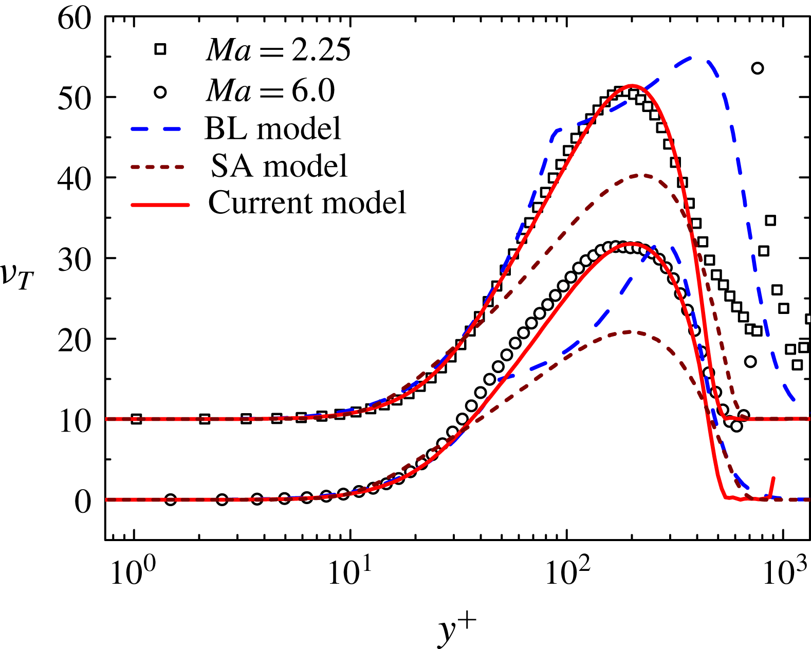
In figure 11, we examine the behaviour of the eddy viscosity
 $\unicode[STIX]{x1D708}_{T}$
, with two DNS profiles from
 $Ma=2.25$
and
 $Ma=6$
at
 $Re_{\unicode[STIX]{x1D70F}}=500$
. It is obvious that the piecewise connected eddy viscosity by the BL model follows the DNS data only in the inner region (i.e.
 $y^{+}\leqslant 50$
), with notable departure in the outer region (the scatter of data towards the free stream is due to the vanishing Reynolds stress and mean shear). In particular, the discrepancy of the BL’s eddy viscosity function at
 $Ma=2.25$
is rather large, while it becomes somewhat reduced at
 $Ma=6$
, explaining its better agreement with the mean velocity observed in figure 7, which is not typical for other
 $Ma$
values. In conclusion, only adjusting the inner function (or parameter
 $\unicode[STIX]{x1D705}$
and
 $A$
) is insufficient to improve the prediction of the mean velocity. Note also that the BL model introduces an arbitrary location
 $y_{c}$
where
 $\unicode[STIX]{x1D708}_{T}$
exhibits a discontinuous derivative. In contrast, the eddy viscosity by the SED-SL model agrees closely with data for the entire boundary layer domain, with a continuous transition from the inner to the outer functions. Also included in figure 11 is the SA model, for which the eddy viscosity is underestimated for both
 $Ma=2.25$
and
 $Ma=6$
, hence leading to underestimation of the mean velocity shown in figures 4 and 6, respectively. Thus, the improvement by SED-SL model is attributed to the correct specification of the eddy viscosity across the entire boundary layer.
Validation of the eddy viscosity function for the BL, SA and SED-SL model by DNS data indicated in table 1, showing that the SED-SL captures the right
 $Ma$
-scaling in describing the variation of the maximum eddy viscosity, which is not the case for the other two models.
5 Conclusion
In this paper, a symmetry-based expression of the stress length, equation (2.7), is tested for compressible flat plate turbulent boundary layers, by formulating an algebraic model (SED-SL) to solve the RANS equation. The model contains only physical parameters (
 $\unicode[STIX]{x1D705}$
,
 $y_{s}^{+}$
and
 $y_{b}^{+}$
) which are invariant for all cases, and the predictions of the mean velocity and temperature profiles of spatially developing CTBLs for a wide range of
 $Ma$
(from 0 to 6) and a restricted range of
 $Re_{\unicode[STIX]{x1D70F}}$
values, for adiabatic as well as heated and cooled walls with a total of 30 mean profiles, are in good agreement with DNS data. Compared to the BL and SA models, the accuracy is notably improved, especially for supersonic and hypersonic CTBLs. It is remarkable that the SED-SL model contains much fewer parameters than the BL and SA models, whose model parameters are of no obvious physical meaning. The comparison clearly demonstrates the efficacy of the multi-layer formula, which captures the right similarity property of the flow in both
 $Re$
and
 $Ma$
. To emphasize, the parameters in the formula were determined by previous study of DNS data (She et al.
Reference She, Chen and Hussain2017), hence the success demonstrates not only the invariance of the length function, but also the universality of the parameters specifying the multi-layer structure.
The symmetry-based approach enables improvement to existing turbulence models, such as the
 $k-\unicode[STIX]{x1D714}$
model (Chen, Hussain & She Reference Chen, Hussain and She2016b
), but here we have proposed a fully theory-based algebraic model. Although the present SED-SL model is not asserted as a sufficiently mature model for CFD applications, the present work demonstrates the feasibility of deriving a high-accuracy model from the multi-layer quantification of wall turbulence. This is clearly shown by comparing SED-SL with BL and SA models for flat plate TBL. At this point, it is right to question the versatility of (any) algebraic model for various flow conditions. The current version of the SED-SL model performs the best for a flat plate CTBL, but a fully operational SED-SL model for general industrial wall flows requires the specification of flow parameters for a variety of benchmark flows, which requires major efforts and will be an interesting topic for future study. In fact, due to the universal character of the wall-induced symmetry constraint, the multi-layer structure is believed to be broadly applicable for many wall flows.
Indeed, the present model can be extended in many ways. For instance, the extension of SED-SL to strong non-equilibrium situations has been accomplished recently to obtain accurate predictions of the streamwise variation of
 $C_{f}$
through TBL transitions (Xiao & She Reference Xiao and She2016). Furthermore, we have identified slight changes in
 $\ell _{0}$
and
 $y_{b}^{+}$
for quantifying the multi-layer structure of flows over airfoils such as NACA0012 and RAE2822 (Xiao & She Reference Xiao and She2017), yielding accurate drag prediction. These (slight) variations of the multi-layer parameters effectively differentiates airfoil flow from a flat plate TBL, which enhances our physical understanding and yields effective engineering models at the same time.
Acknowledgements
We thank B. Wu for helpful discussions. This work is supported by National Natural Science Fund (of China) 11452002, 11221062 and by MOST 973 project 2009CB724100 of China.



