1 Introduction
Pipes conveying fluid are used in common heat exchangers, the oil and gas industry and nuclear power engineering. The flow is turbulent and the pipes are typically long and flexible, causing flow-induced vibrations that may further destabilize the flow and consequently the pipe structure in a nonlinear feedback loop. In previous studies, the focus has been mainly on the pipe dynamics using approximate flow models based on simple one-dimensional flow assumptions (Paidoussis Reference Paidoussis1998, Reference Paidoussis2004). Recently, Xie et al. (Reference Xie, Zheng, Triantafyllou, Constantinides and Karniadakis2016) performed the first direct numerical simulation (DNS) of transitional flow in a vibrating pipe, investigating specific flow patterns inside the pipe and correlating them to periodic and chaotic responses of the induced pipe motion. Pittard et al. (Reference Pittard, Evans, Maynes and Blottera2004) conducted both experimental measurements and coarse large eddy simulations of relatively short pipes and obtained a strong correlation between pipe vibration and flow rate, suggesting that pressure fluctuations on the pipe wall have a near quadratic relationship with the flow rate. This is a very interesting study but the large eddy simulation (LES) presented clearly under-resolved the flow in the Reynolds number regime considered (more than 100 000) so no details of the structure of the turbulence, e.g. mean velocity profiles or other statistics, were reported. To the best of our knowledge, there have not been any previous systematic investigations on the effect of pipe motion on the turbulence statistics in periodic vibration. In the current work, we simplify somewhat the problem and consider prescribed oscillatory pipe motion in order to study in detail the turbulent flow inside the pipe similar to the work of Wu & Moin (Reference Wu and Moin2008), who considered DNS of a stationary pipe flow. In ongoing work, we have also simulated the effects of free pipe vibration and we will report such results in the future. In addition, in the current paper we present for first time a potentially very effective numerical approach to wall-bounded high Reynolds number turbulence simulation based on a new concept of entropy-based eddy viscosity to stabilize the simulations, analogous to large eddy simulations as we explain below.
In conventional large eddy simulation (LES), the large resolved scales are typically separated from the small scales by proper filtering of the velocity field, with the size of the filter a function of the grid size. The under-resolved Reynolds stresses are modelled by a linear relationship of an ‘eddy viscosity’ times the strain rate tensor of the resolved field. Such a simple algebraic (subgrid scale) model is isotropic, which is a statistically correct assumption for homogeneous turbulence at high Reynolds number (Pope Reference Pope2000). However, in practical numerical simulations these subgrid models depend strongly on the type of flow considered as well as the numerical method for discretization. Since their introduction several decades ago, a considerable number of subgrid models have been proposed in the literature (Lesieur & Metais Reference Lesieur and Metais1996; Pope Reference Pope2004; Sagaut Reference Sagaut2006). The simplest and most widely used is the classical Smagorinsky model (Smagorinsky Reference Smagorinsky1963; Bardina, Ferziger & Reynolds Reference Bardina, Ferziger and Reynolds1980; Germano et al. Reference Germano, Piomelli, Moin and Cabot1991; Lilly Reference Lilly1992) and its variants (Sarghini, Piomelli & Balaras Reference Sarghini, Piomelli and Balaras1999; Meneveau & Katz Reference Meneveau and Katz2000), which are reminiscent of Boussinesq’s hypothesis, which assumes that the anisotropic residual stress is proportional to the traceless mean strain rate tensor.
From the mathematical perspective, the filtering of the small-scale and high frequency oscillations of the velocity field in a numerical simulation can be regarded as stabilization procedure of the computation. To this end, the ‘implicit’ LES (ILES) proposed in Boris et al. (Reference Boris, Grinstein, Oran and Kolbe1992), Fureby & Grinstein (Reference Fureby and Grinstein1999), Geurts (Reference Geurts2004), Grinstein, Margonin & Rider (Reference Grinstein, Margonin and Rider2007), solves the unfiltered Navier–Stokes equations using especially designed monotone algorithms, often used in high-speed aerodynamics. Similarly, in the framework of high-order methods, e.g. in spectral and spectral element methods, the concept of spectral vanishing viscosity (SVV) was introduced in order to deal with the loss of monotonicity in the numerical solution of the inviscid Burgers equation in Tadmor (Reference Tadmor1989), and this concept was later introduced for the numerical solution of the Navier–Stokes equations in Karamanos & Karniadakis (Reference Karamanos and Karniadakis2000), Xu & Pasquetti (Reference Xu and Pasquetti2004). Hughes et al. (Reference Hughes, Feijóo, Mazzei and Quincy1998) emphasized that there is an intriguing relationship between the stabilization of a numerical method and the subgrid modelling of multi-scale phenomena such as in turbulent flows. Based on this idea, they proposed the variational multi-scale (VMS) models for LES in Hughes, Oberai & Mazzei (Reference Hughes, Oberai and Mazzei2001).
More recently, Guermond (Reference Guermond2008), Guermond, Pasquetti & Popov (Reference Guermond, Pasquetti and Popov2011c
), Guermond, Larios & Thompson (Reference Guermond, Larios and Thompson2015) proposed the so-called ‘entropy-viscosity method’ (EVM) for stabilizing conservation laws based on the concept of the entropy residual. Specifically, they monitor the local kinetic energy balance and introduce a localized dissipation in these regions, which is proportional to the local residual that expresses a potential violation of the local conservation law. They termed this local dissipation ‘entropy viscosity’ as it reflects the entropy production in that region, analogous to the entropy production in conservation laws in high-speed aerodynamics. While most of the applications of EVM have been for simple solutions to demonstrate the preservation of monotonicity of the numerical solutions, Guermond, Nazarov & Popov (Reference Guermond, Nazarov and Popov2011a
), Nazarov, Guermond & Popov (Reference Nazarov, Guermond and Popov2011), Nazarov & Larcher (Reference Nazarov and Larcher2017) have applied EVM to the compressible Euler equation, Guermond et al. (Reference Guermond, Larios and Thompson2015) also applied it to the incompressible homogeneous isotropic turbulence problem. However, to the best of our knowledge, EVM has not been employed in simulating inhomogeneous turbulent flows, where the presence of the wall affects greatly the local dissipation due to the steep boundary layer structure with possible under-resolution of the simulation there. Specifically, the parametrization of the model has not been studied systematically, especially in the context of resolving internal turbulent flows. We have developed the EVM method in the context of the spectral element method (Karniadakis & Sherwin Reference Karniadakis and Sherwin2005) and have pursued a systematic investigation of the accuracy of the simulation in pipe turbulent flows reported here as well as external flows in ongoing work. Specifically, we have obtained the value of the main free parameter
 $\unicode[STIX]{x1D6FC}$
(see (2.3)) by an analogy between the entropy viscosity and the eddy viscosity of the Smagorinsky model.
This paper is organized as follows. In § 2 we introduce EVM and its implementation, and in § 3 we present a systematic validation of EVM by simulating turbulent flow in a stationary pipe at
 $Re_{D}=5300$
and
 $Re_{D}=44\,000$
and comparing against the highly resolved simulations of Wu & Moin (Reference Wu and Moin2008); we also make some comparisons against the eddy viscosity obtained by the Smagorinsky model. In § 4 we present the simulation results of turbulent flow in a pipe undergoing a standing-wave vibration at
 $Re_{D}=5300$
, including turbulent statistics, turbulence budgets, flow visualization as well as two-point correlations. We end with a summary of our results. The two appendices include more results from validation studies.
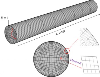
Spectral element mesh for flow in a pipe. There are 576 quadrilateral prismatic elements. Fourier discretization is used along the
 $z$
direction.

2 Computational methods
We consider incompressible flow in a cylindrical pipe in the domain shown in figure 1 with spectral element discretization based on each (
 $x{-}y$
) plane and a Fourier expansion along the flow (
 $z-$
) direction. The governing equations are the continuity and Navier–Stokes equations, which we discretize here in Cartesian coordinates:
 $$\begin{eqnarray}\displaystyle & \displaystyle \unicode[STIX]{x1D735}\boldsymbol{\cdot }\mathit{u}=0, & \displaystyle\end{eqnarray}$$
 $$\begin{eqnarray}\displaystyle & \displaystyle {\displaystyle \frac{\unicode[STIX]{x2202}\mathit{u}}{\unicode[STIX]{x2202}t}}+\mathit{u}\boldsymbol{\cdot }\unicode[STIX]{x1D735}\mathit{u}=-\unicode[STIX]{x1D735}p+{\displaystyle \frac{1}{Re}}\unicode[STIX]{x1D6FB}^{2}\mathit{u}+\unicode[STIX]{x1D735}\boldsymbol{\cdot }[\unicode[STIX]{x1D708}_{t}(\unicode[STIX]{x1D735}\mathit{u}+\unicode[STIX]{x1D735}^{\text{T}}\mathit{u})]+\mathit{F}, & \displaystyle\end{eqnarray}$$
the scalar
 $\unicode[STIX]{x1D708}_{t}$
is the so-called ‘entropy viscosity’, similar to the eddy viscosity in LES models. Here, to simplify the calculation we will lump the value of the entropy viscosity into a single number computed over an entire spectral element. We have modified the original formula proposed by Guermond et al. (Reference Guermond, Pasquetti and Popov2011c
, Reference Guermond, Larios and Thompson2015) and we propose the following formula to compute the entropy viscosity in each element
 $K$
at the collocation points
 $ijm$
:
 $$\begin{eqnarray}\unicode[STIX]{x1D708}_{t}|_{K}=\text{min}\left\{\boldsymbol{\unicode[STIX]{x1D6FD}}\Vert \mathit{u}\Vert _{L^{\infty }(K)}\unicode[STIX]{x1D6FF}_{K},\unicode[STIX]{x1D736}{\displaystyle \frac{\Vert R_{ijm}^{K}(\mathit{u})\Vert _{L^{\infty }(K)}}{\Vert E_{ijm}^{K}(\mathit{u})-\bar{E}(\mathit{u})\Vert _{L^{\infty }(\unicode[STIX]{x1D6FA})}}}\unicode[STIX]{x1D6FF}_{K}^{2}\right\}\!,\end{eqnarray}$$
where we use the maximum norm
 $L^{\infty }(K)$
over an element
 $K$
or
 $L^{\infty }(\unicode[STIX]{x1D6FA})$
over the entire domain
 $\unicode[STIX]{x1D6FA}$
. We define the various quantities as follows:
 $$\begin{eqnarray}E_{ijm}^{K}(\mathit{u})={\displaystyle \frac{1}{2}}(\boldsymbol{u}_{ijm}^{K}-\overline{\boldsymbol{u}}(\unicode[STIX]{x1D6FA}))^{2},\quad \bar{E}(\mathit{u})={\displaystyle \frac{\displaystyle \int _{\unicode[STIX]{x1D6FA}}E_{ijm}^{K}(\mathit{u})\boldsymbol{\cdot }\text{d}\boldsymbol{X}}{\displaystyle \int _{\unicode[STIX]{x1D6FA}}\,\text{d}\boldsymbol{X}}},\end{eqnarray}$$
 $$\begin{eqnarray}R_{ijm}^{K}(\mathit{u})=\mathit{u}\boldsymbol{\cdot }\left.\left({\displaystyle \frac{\unicode[STIX]{x2202}\mathit{u}}{\unicode[STIX]{x2202}t}}+\mathit{u}\boldsymbol{\cdot }\unicode[STIX]{x1D735}\mathit{u}+\unicode[STIX]{x1D735}p-{\displaystyle \frac{1}{Re}}\unicode[STIX]{x1D6FB}^{2}\mathit{u}-\mathit{f}\right)\right|_{ijm}^{K},\end{eqnarray}$$
where
 $\unicode[STIX]{x1D6FF}_{K}$
is the minimum distance between two quadrature points in element
 $K$
,
 $\overline{\boldsymbol{u}}(\unicode[STIX]{x1D6FA})$
are global mean values of
 $\boldsymbol{u}$
. As shown in (2.3), the entropy viscosity is a combination of two terms corresponding to two parameters
 $\unicode[STIX]{x1D6FC}$
and
 $\unicode[STIX]{x1D6FD}$
. The first term is the upper bound of the entropy viscosity and corresponds to a first-order upwind scheme; on a uniform mesh, its value is
 $\unicode[STIX]{x1D6FD}=1/2$
, which is equivalent to the numerical viscosity of a first-order upwind scheme, see Guermond, Pasquetti & Popov (Reference Guermond, Pasquetti and Popov2011b
). Hence, the magnitude of entropy viscosity will never exceed the numerical viscosity of the corresponding first-order upwind scheme. We note that in the implementation of (2.2), since we consider constant
 $\unicode[STIX]{x1D708}_{t}$
per each element
 $K$
, we follow element by element integration by parts, the weak form of (2.2) is greatly simplified. We note that the choice of
 $L^{\infty }(\unicode[STIX]{x1D6FA})$
in the above equations is valid only if the flow characteristics are relatively homogeneous. In strongly inhomogeneous flows, an appropriately defined subdomain should be employed.
Our method differs, however, from the one proposed originally in Guermond et al. (Reference Guermond, Pasquetti and Popov2011b
,Reference Guermond, Pasquetti and Popov
c
) with respect to the second term since the parameter
 $\unicode[STIX]{x1D736}$
in (2.3) is no longer an adjustable constant. Instead, based on physical arguments, we can set a fixed value by analogy with the Smagorinsky eddy-viscosity model as follows. In (2.5) and (2.4),
 $R(\mathit{u})$
and
 $E(\mathit{u})$
have units that are
 $\text{m}^{2}~\text{s}^{-3}$
and
 $\text{m}^{2}~\text{s}^{-2}$
, which are the same as that of the turbulence dissipation rate
 $\unicode[STIX]{x1D716}$
and turbulence kinetic energy
 $k$
, respectively, therefore intuitively, we propose the following approximation:
 $$\begin{eqnarray}{\displaystyle \frac{\Vert R_{ijm}^{K}(\mathit{u})\Vert _{L^{\infty }(K)}}{\Vert E_{ijm}^{K}(\mathit{u})-\bar{E}(\mathit{u})\Vert _{L^{\infty }(\unicode[STIX]{x1D6FA})}}}\approx C_{x}{\displaystyle \frac{\unicode[STIX]{x1D716}}{k}},\end{eqnarray}$$
where
 $C_{x}$
is a constant. Then by substituting equation (2.6) into (2.3), and assuming that the entropy viscosity obtained from (2.3) is equal to the eddy viscosity of the Smagorinsky model, we obtain:
 $$\begin{eqnarray}\unicode[STIX]{x1D6FC}C_{x}{\displaystyle \frac{\unicode[STIX]{x1D716}}{k}}(\unicode[STIX]{x1D6FF}_{K})^{2}\approx (C_{s}\unicode[STIX]{x1D6FF}_{K})^{2}\overline{\unicode[STIX]{x1D64E}}.\end{eqnarray}$$
In the above equation, the right-hand side is the eddy viscosity of the Smagorinsky model, where
 $\overline{\unicode[STIX]{x1D64E}}=(2\overline{\unicode[STIX]{x1D64E}}_{ij}\,\overline{\unicode[STIX]{x1D64E}}_{ij})$
is defined based on the rate-of-strain tensor, and
 $$\begin{eqnarray}C_{s}={\displaystyle \frac{1}{\unicode[STIX]{x03C0}}}\left({\displaystyle \frac{2}{3C_{K}}}\right)^{3/4}\end{eqnarray}$$
is the Smagorinsky coefficient, where
 $C_{K}=1.5$
is the Kolmogorov constant. Equation (2.7) could be simplified as:
 $$\begin{eqnarray}\unicode[STIX]{x1D6FC}\approx {\displaystyle \frac{(C_{s})^{2}}{C_{x}}}\overline{\unicode[STIX]{x1D64E}}{\displaystyle \frac{k}{\unicode[STIX]{x1D716}}}.\end{eqnarray}$$
Furthermore, Pope (Reference Pope2000, p. 589) gives an estimation that
 $$\begin{eqnarray}{\displaystyle \frac{\langle \overline{\unicode[STIX]{x1D64E}}^{2}\rangle ^{1/2}k}{\unicode[STIX]{x1D716}}}\approx \unicode[STIX]{x03C0}^{2/3}\left({\displaystyle \frac{3}{2}}C_{K}\right)^{1/2}\left({\displaystyle \frac{\unicode[STIX]{x1D6E5}}{L}}\right)^{-2/3},\end{eqnarray}$$
where
 $\unicode[STIX]{x1D6E5}$
is a filter width and
 $L=k^{3/2}/\unicode[STIX]{x1D716}$
is the flow length scale. Note that, in the above equation, we assume
 $\langle \overline{\unicode[STIX]{x1D64E}}^{2}\rangle ^{1/2}\approx \overline{\unicode[STIX]{x1D64E}}$
. By substituting (2.8), (2.10) into (2.9), we obtain,
 $$\begin{eqnarray}\unicode[STIX]{x1D6FC}=\left({\displaystyle \frac{3}{2}}C_{K}C_{x}\right)^{-1}\unicode[STIX]{x03C0}^{-4/3}\left({\displaystyle \frac{\unicode[STIX]{x1D6E5}}{L}}\right)^{-2/3}.\end{eqnarray}$$
In (2.11), the constants
 $\unicode[STIX]{x1D6E5}/L$
and
 $C_{x}$
need to be estimated. We also note that the above arguments are somewhat ad hoc, and hence this may be a limitation of the current approach, since they are related to a local assumption of homogeneity.
Pope (Reference Pope2000, p. 187) writes that the length scale splitting the inertial subrange and energy-containing range is defined as
 $L_{EI}=(1/6)L$
. Moreover, Pope (Reference Pope2000, p. 560) recommends that for LES, the filter width
 $\unicode[STIX]{x1D6E5}$
should be fine enough to resolve 80 % of the energy, which corresponds to the following estimation using Pope (Reference Pope2000, p. 577),
 $$\begin{eqnarray}{\displaystyle \frac{\unicode[STIX]{x1D6E5}}{L}}={\displaystyle \frac{1}{12}}.\end{eqnarray}$$
Next, in particular, for homogeneous isotropic turbulence (HIT), if we assume
 $C_{x}=1$
, we could obtain a specific value for
 $\unicode[STIX]{x1D6FC}$
:
 $$\begin{eqnarray}\unicode[STIX]{x1D6FC}\approx 0.5.\end{eqnarray}$$
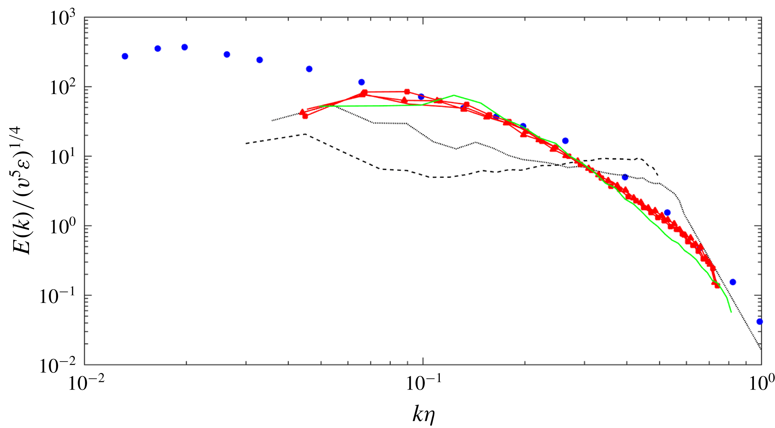
Indeed, in appendix A we demonstrate that
 $\unicode[STIX]{x1D6FC}=0.5$
works well for HIT, and the simulation results do not seem to be very sensitive to the specific value of
 $\unicode[STIX]{x1D6FC}$
as long as it is in a range close to 0.5. As shown in previous studies for LES of wall-bounded turbulence, the value of
 $C_{s}=0.17$
leads to excessive dissipation so lower values, e.g.
 $C_{s}=0.1$
, are typically used as reported in Lesieur & Metais (Reference Lesieur and Metais1996). This range of values would lead to an adjustment of our parameter
 $\unicode[STIX]{x1D6FC}$
to be two orders of magnitude smaller (quadratic dependence on
 $C_{s}$
), and indeed systematic simulations for turbulent channel and pipe flow indicated that a value of 0.005 (
 $C_{x}=100$
) leads to best results. This issue is further investigated in § 3.3 and appendix B.
3 Turbulent flow in a stationary pipe
In this section, we present the EVM simulations of fully turbulent flow in a stationary pipe at
 $Re_{D}=5300$
and
 $Re_{D}=44\,000$
, which were first considered in high-resolution DNS by Wu & Moin (Reference Wu and Moin2008). The results of this section, together with the results presented in appendices A and B, are included for validation of our method as well as for comparison with the results presented in the next section for turbulent flow in a vibrating pipe.
3.1 Simulation details
For both Reynolds number simulations, we use the same computational domain with a length
 $L_{z}=8D$
, where
 $D$
is the pipe diameter, see figure 1. For
 $Re_{D}=5300$
, the two-dimensional cross-section
 $x{-}y$
is partitioned into 576 quadrilateral spectral elements and in each element we employ fourth-order Jacobi polynomials while along the flow (homogeneous and periodic) direction we employ 128 Fourier planes (64 Fourier modes). Correspondingly, for
 $Re_{D}=44\,000$
we employ eighth-order Jacobi polynomials in the
 $x{-}y$
plane and 512 Fourier planes (256 Fourier modes) along the flow direction. The selected discretizations lead to a resolution that in the radial direction, for both Reynolds numbers, we have
 $(1-r)^{+}<1$
for the first grid point away from the pipe wall while along the azimuthal direction we have
 $\unicode[STIX]{x1D6E5}(R\unicode[STIX]{x1D703})^{+}=4.44$
and
 $\unicode[STIX]{x1D6E5}(R\unicode[STIX]{x1D703})^{+}=16.02$
for
 $Re_{D}=5300$
and
 $Re_{D}=44\,000$
, respectively. Also, along the
 $z$
direction,
 $z^{+}=11.33$
and
 $z^{+}=71.38$
for
 $Re_{D}=5300$
and
 $Re_{D}=44\,000$
, respectively. The number of grid points for the low Reynolds number is 114 times less than the DNS simulation of Wu & Moin (Reference Wu and Moin2008) and 33 times less than the corresponding DNS of Wu & Moin (Reference Wu and Moin2008) at the high Reynolds number. These resolutions are also less than Piomelli’s (Reference Piomelli2008) estimation of the resolution requirements for a near-wall-resolved LES, scaling approximately as
 $O(Re^{1.8})$
. The time step for the simulation at the smaller
 $Re_{D}$
is fixed at
 $\unicode[STIX]{x0394}t=1\times 10^{-3}$
, while
 $\unicode[STIX]{x0394}t=3\times 10^{-4}$
for the larger
 $Re_{D}$
. Extensive resolution studies have been conducted by increasing the order of spectral polynomial in each element; for details see appendix C. Here
 $r$
is the radial coordinate normalized by
 $R$
measured from the pipe centreline, therefore
 $(1-r)$
represents the normalized distance from the pipe wall. Superscript
 $^{+}$
denotes normalizing by wall units
 $\unicode[STIX]{x1D708}/u_{\unicode[STIX]{x1D70F}}$
, where
 $\unicode[STIX]{x1D708}$
is the kinematic viscosity and
 $u_{\unicode[STIX]{x1D70F}}$
is the frictional velocity.
During the simulation, a dynamically adjusted driving force is employed to maintain the bulk velocity at
 $\overline{\mathit{u}}_{\mathit{bulk}}=1$
. Specifically, we used
 $\mathit{F}=(\overline{\mathit{u}}_{\mathit{bulk}}-\overline{\mathit{u}}_{\mathit{inst}})/\triangle t$
, where
 $\overline{\mathit{u}}_{\mathit{inst}}$
is the bulk velocity from the instantaneous solution. In our configuration, the target Kármán numbers,
 $R^{+}=R/u_{\unicode[STIX]{x1D70F}}$
, are
 $R^{+}=180,1142$
, based on the balance of forces along the streamwise (
 $z$
) direction, thus the driving forces should be
 $\mathit{F}_{obj}=(4R^{+}/Re_{D})^{2}=0.0185,0.0108$
, respectively. In our simulations, the standard deviation of
 $\mathit{F}$
from
 $\mathit{F}_{obj}$
is less than 2 %.
To speed up the transition from laminar flow to turbulent flow, in the initial stage that is approximately
 $30D/\overline{\mathit{u}}_{\mathit{bulk}}$
, extra sinusoidal body forces were employed. Statistics were collected after the turbulent flow was fully developed. The sampling time durations were
 $100D/\overline{\mathit{u}}_{\mathit{bulk}}$
and
 $50D/\overline{\mathit{u}}_{\mathit{bulk}}$
for the simulation of
 $Re_{D}=5300$
and
 $Re_{D}=44\,000$
, respectively, comparable to the sampling times of DNS. To compare with the DNS solutions of Wu & Moin (Reference Wu and Moin2008), we placed
 $64\times 64$
probes in every
 $(x,y)$
plane. These probes were distributed uniformly on the
 $\unicode[STIX]{x1D703}$
coordinates and clustered towards the wall. The statistical samples were averaged in time and along the two homogeneous directions
 $(z,\unicode[STIX]{x1D703})$
; in particular, the second-order statistics are calculated as follows,
 $$\begin{eqnarray}\overline{u_{z}^{\prime }u_{z}^{\prime }}=\overline{u_{z}u_{z}}-\overline{u_{z}}\cdot \overline{u_{z}},\end{eqnarray}$$
where the overline denotes averaging both along the homogeneous spatial directions and in time.
3.2 Comparisons of EVM simulations against DNS
The accuracy of the EVM simulations is demonstrated by comparison with the well-known DNS results of Wu & Moin (Reference Wu and Moin2008). The EVM results of the friction velocities are
 $u_{\unicode[STIX]{x1D70F}}=0.0681$
for
 $Re_{D}=5300$
and
 $u_{\unicode[STIX]{x1D70F}}=0.0529$
for
 $Re_{D}=44\,000$
, which compare well with the DNS results (Wu & Moin Reference Wu and Moin2008) of
 $0.0684$
and
 $0.0519$
, respectively, with the differences being less than 2 %.
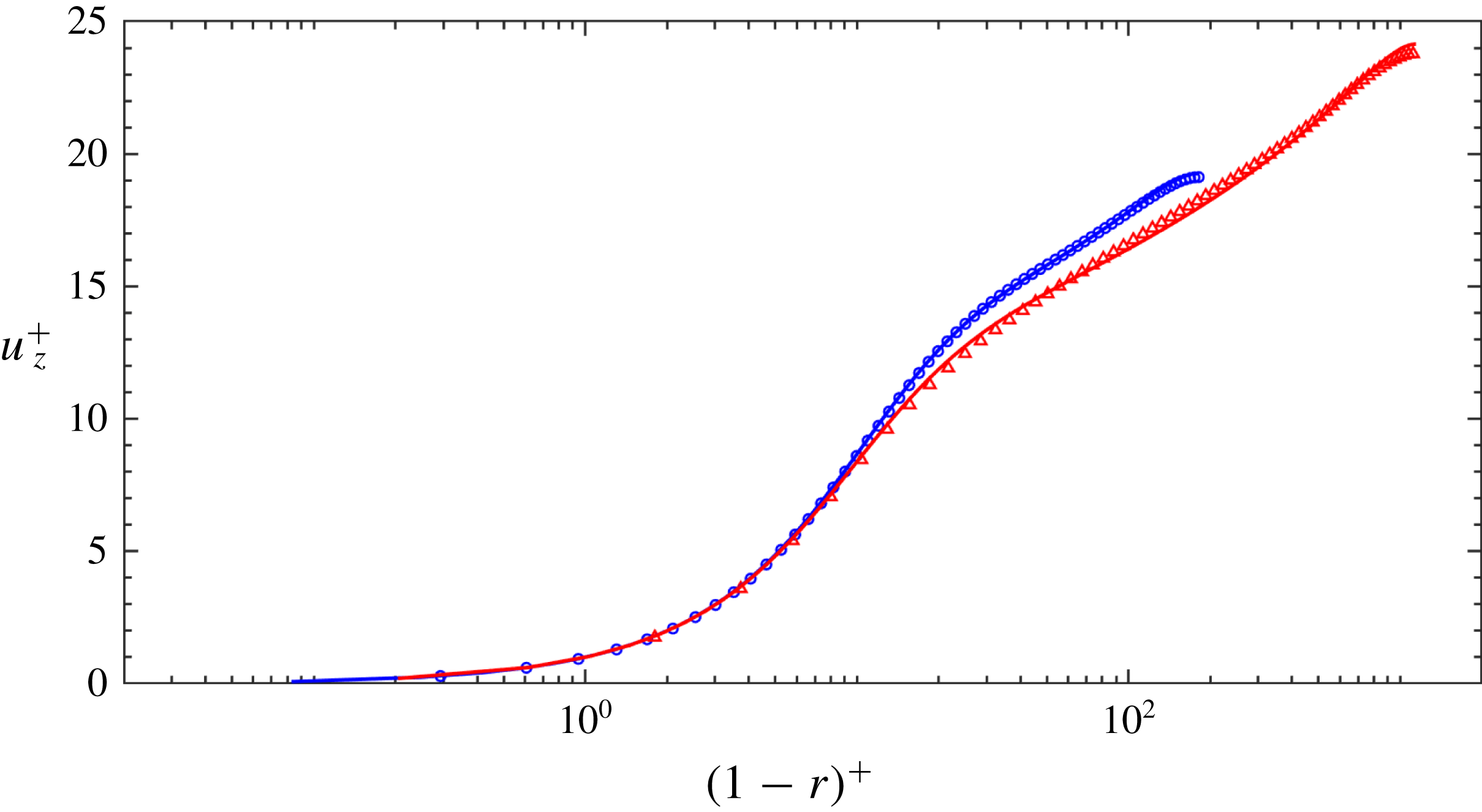
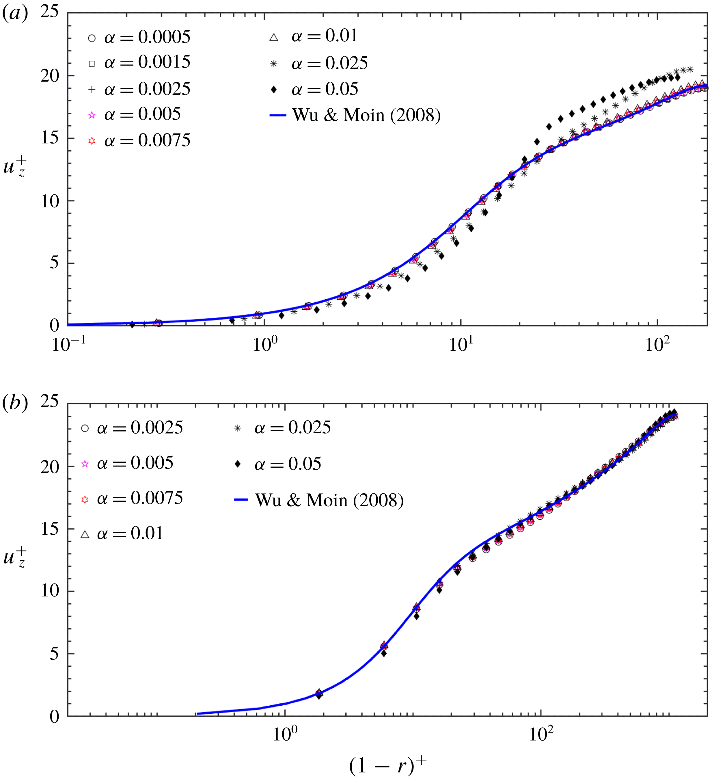
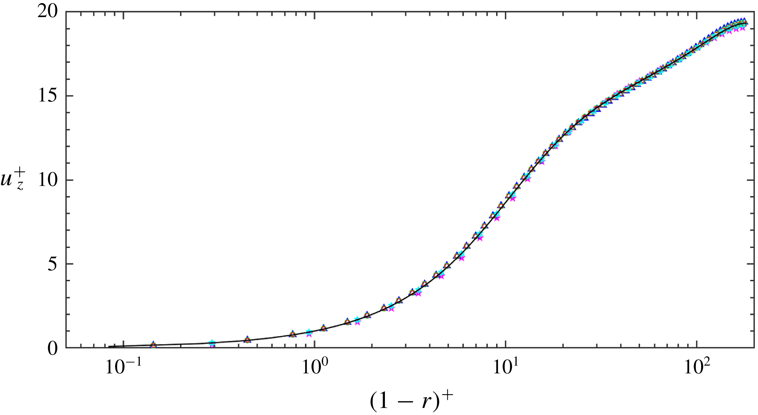
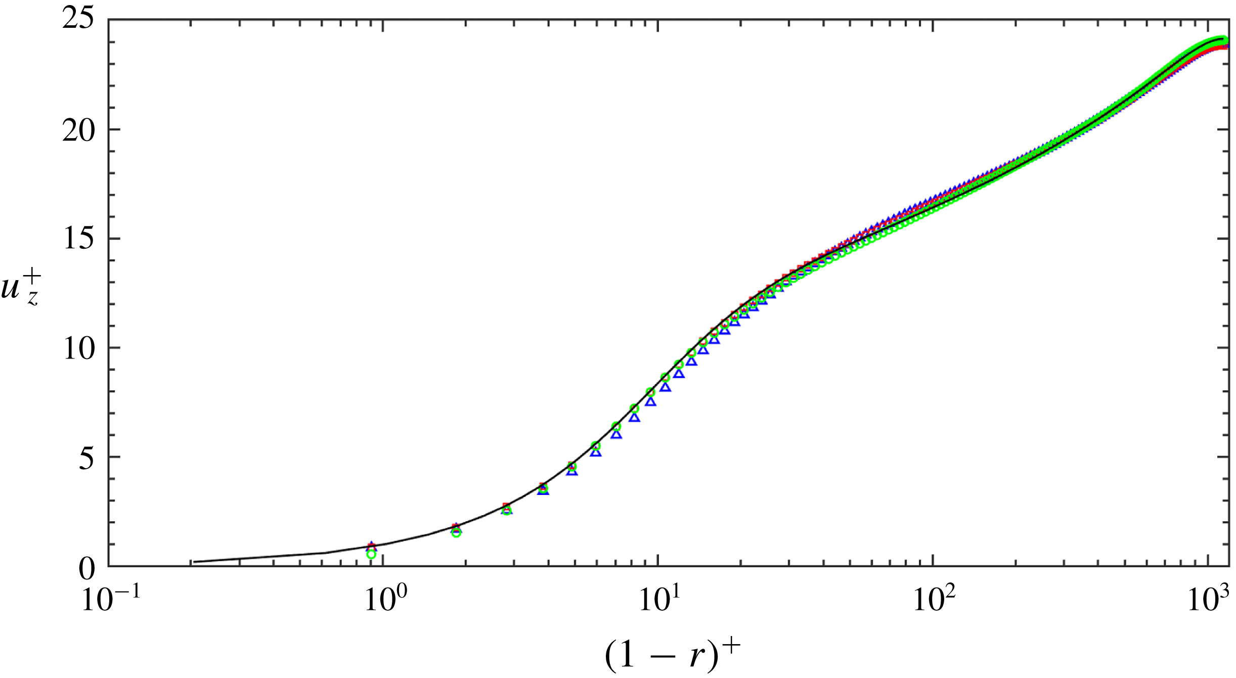
Mean axial velocity
 $\overline{u_{z}}^{+}$
as a function of
 $(1-r)$
. Blue solid line: Wu & Moin (Reference Wu and Moin2008) at
 $Re_{D}=5300$
; red solid line: Wu & Moin (Reference Wu and Moin2008) at
 $Re_{D}=44\,000$
; blue circles: current EVM at
 $Re_{D}=5300$
; red triangles: current EVM at
 $Re_{D}=44\,000$
.

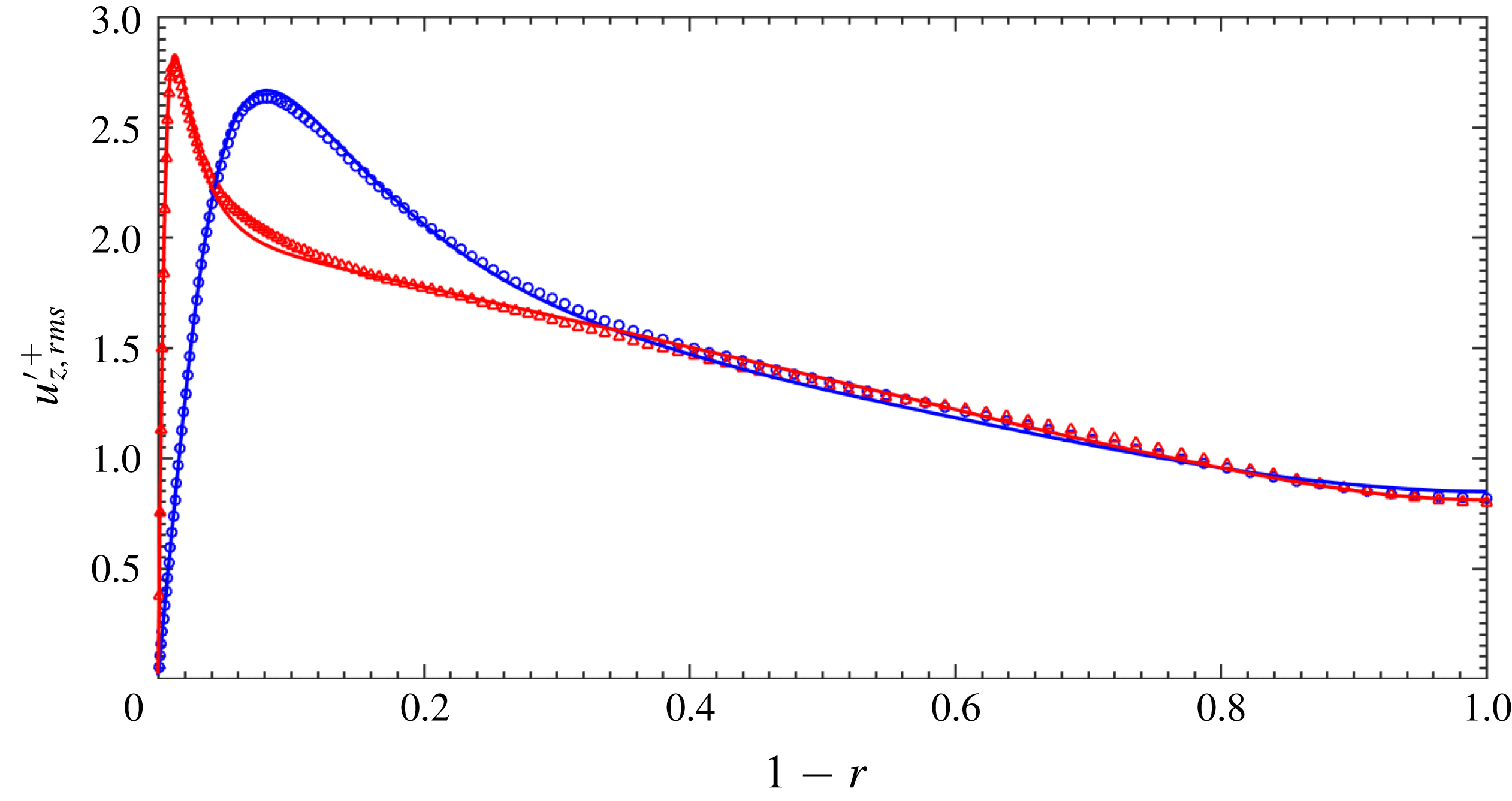
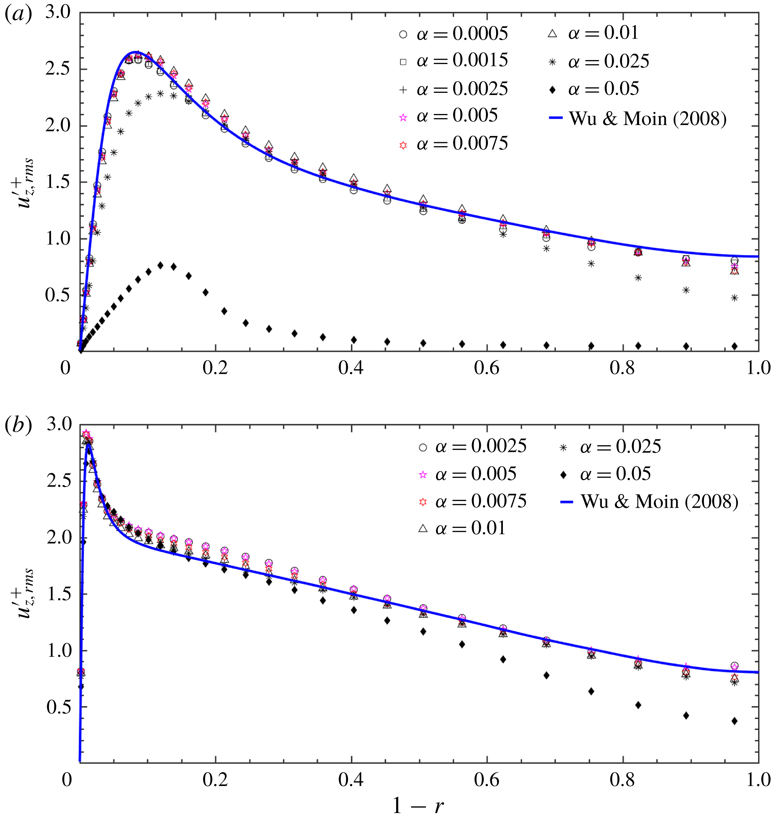
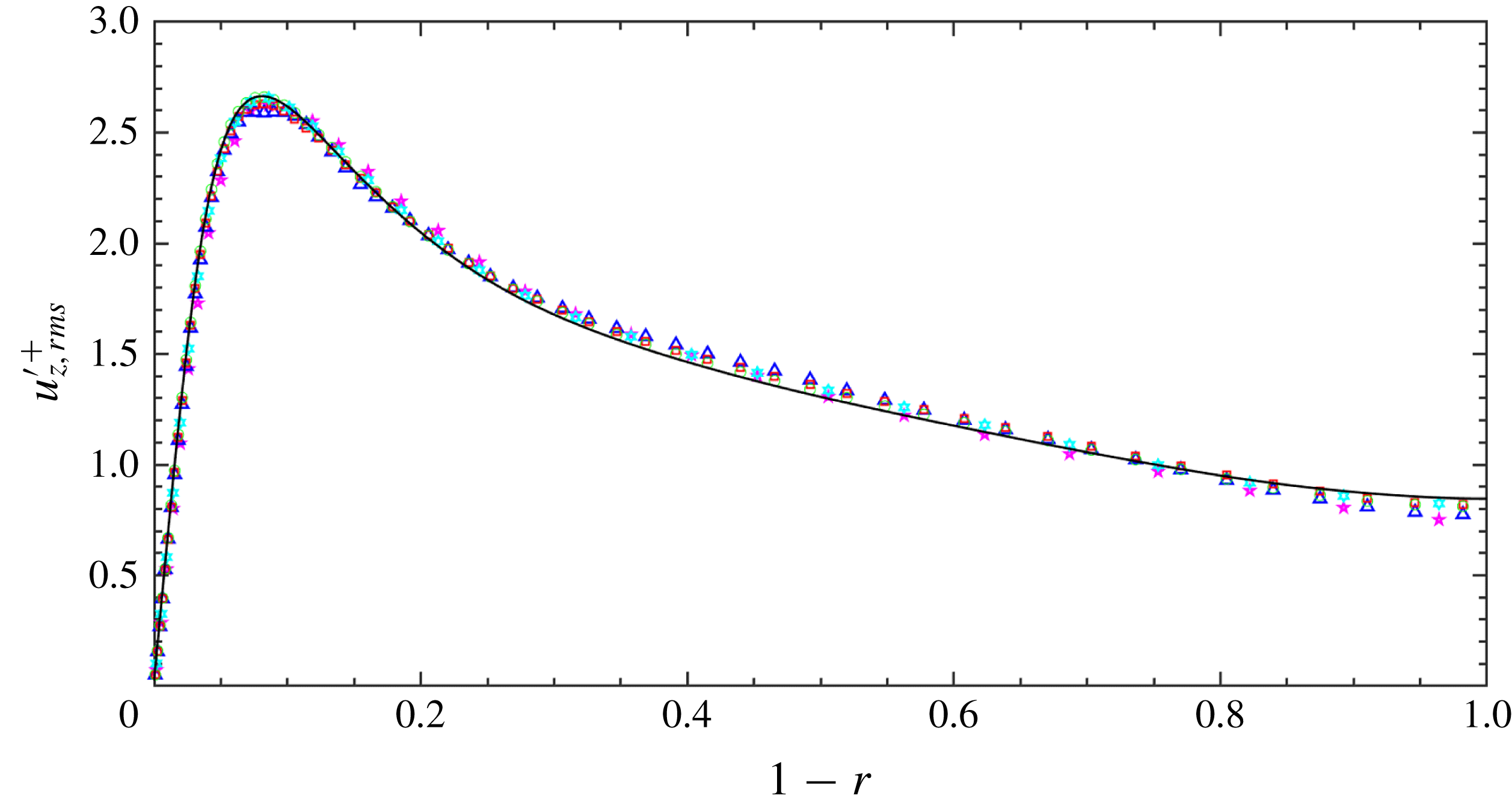
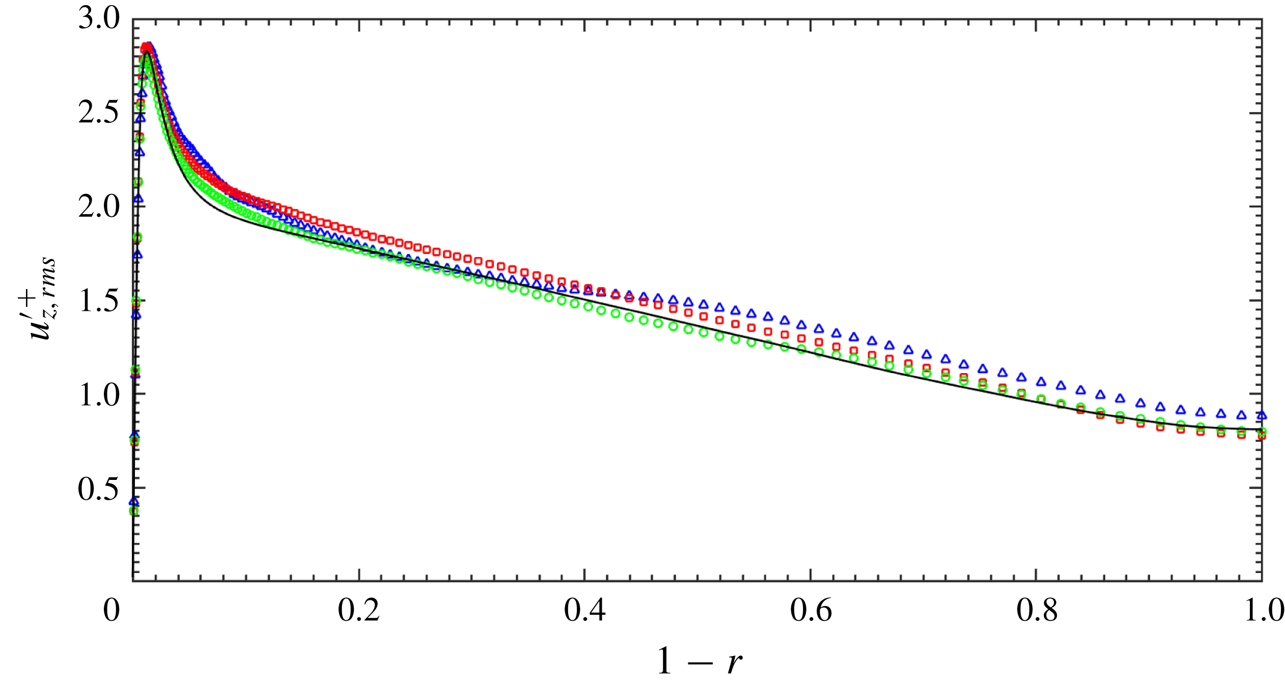
Axial turbulence intensity
 $u_{z,rms}^{\prime +}$
as a function of
 $(1-r)$
. For details see figure 2.

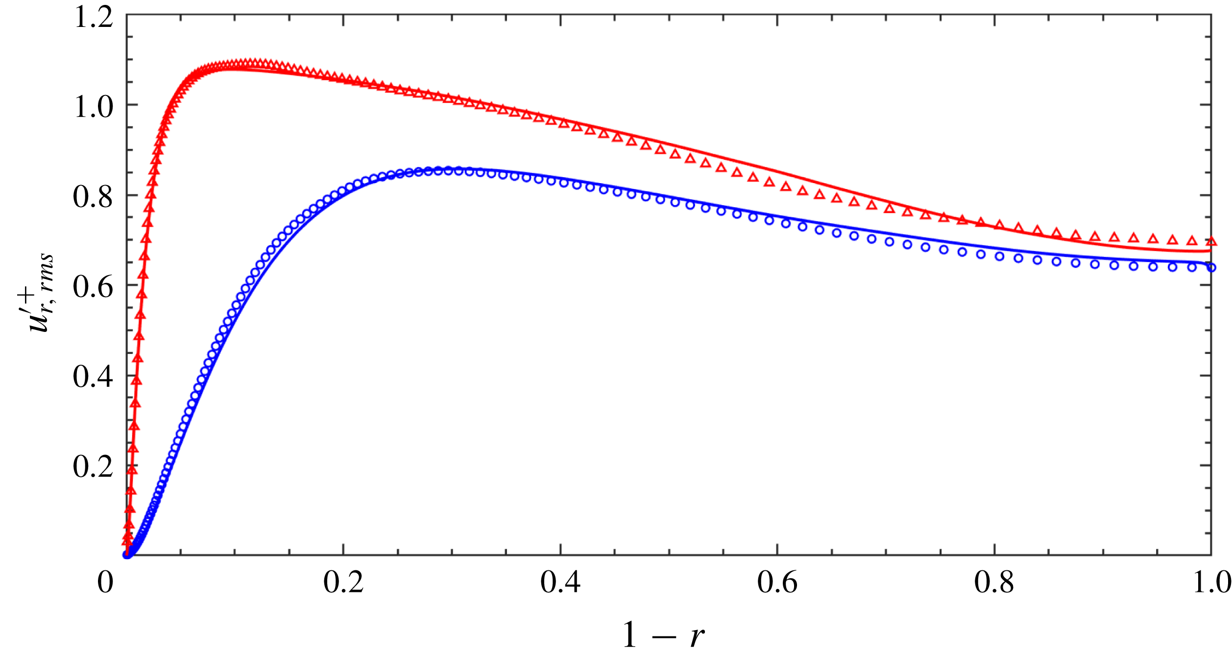
Wall-normal turbulence intensity
 $u_{r,rms}^{\prime +}$
as a function of
 $(1-r)$
. For details see figure 2.

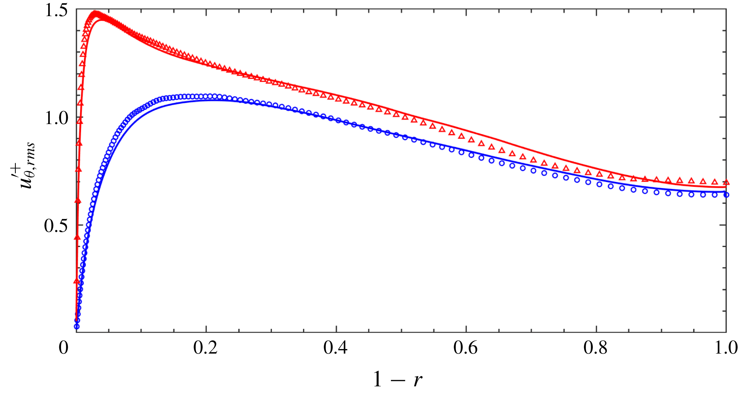
Azimuthal turbulence intensity
 $u_{\unicode[STIX]{x1D703},rms}^{\prime +}$
as a function of
 $(1-r)$
. For details see figure 2.

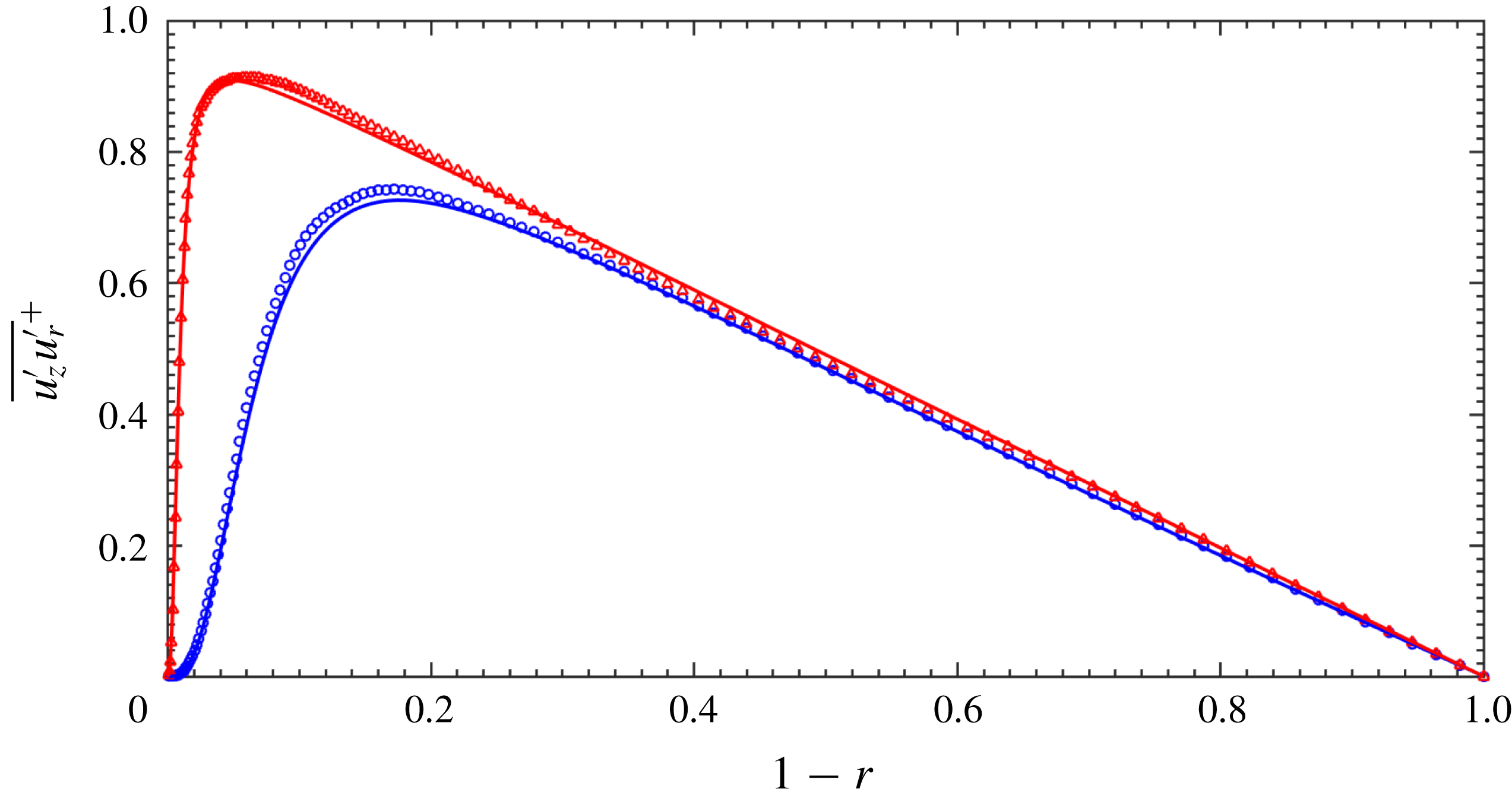
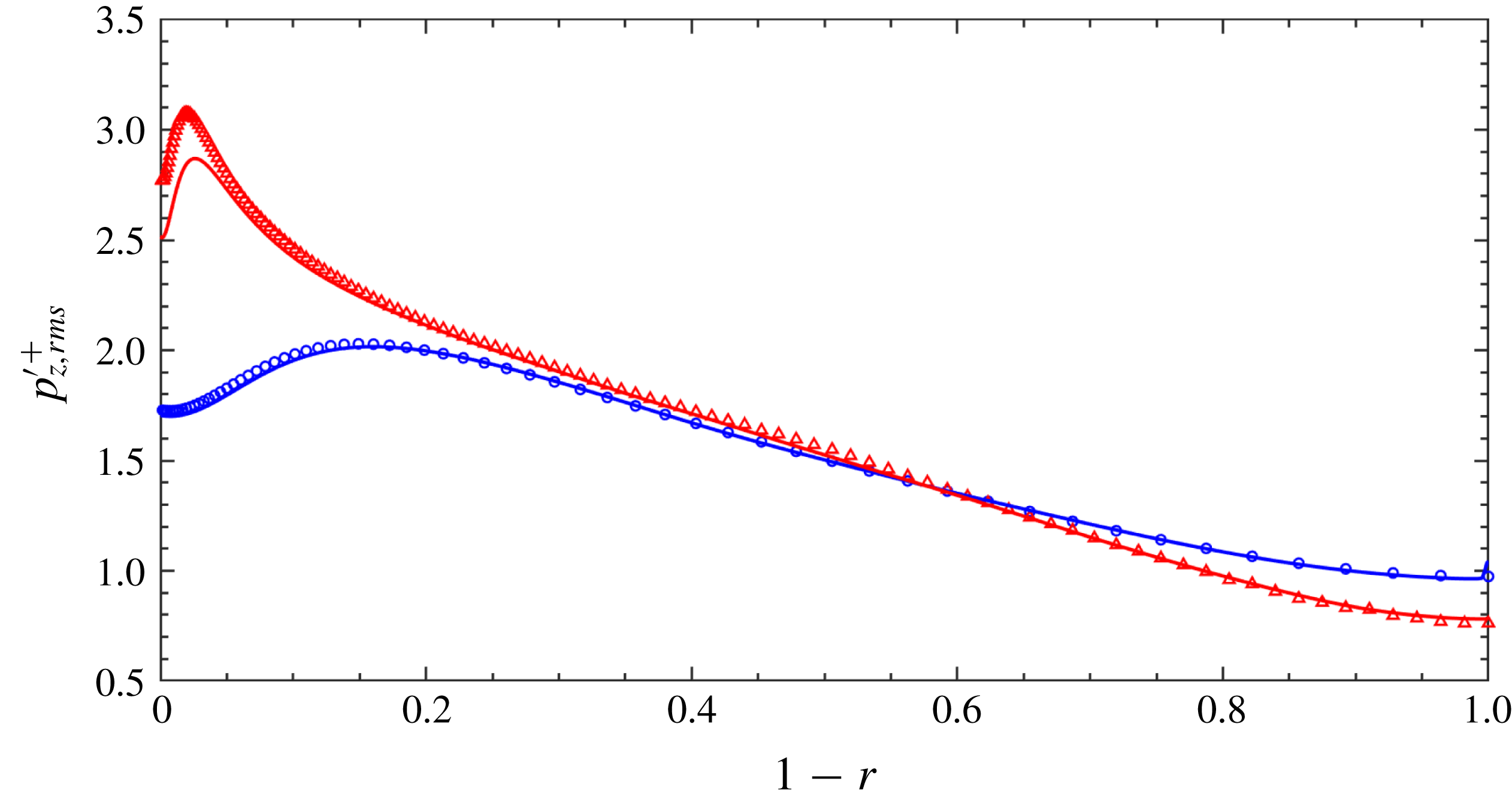
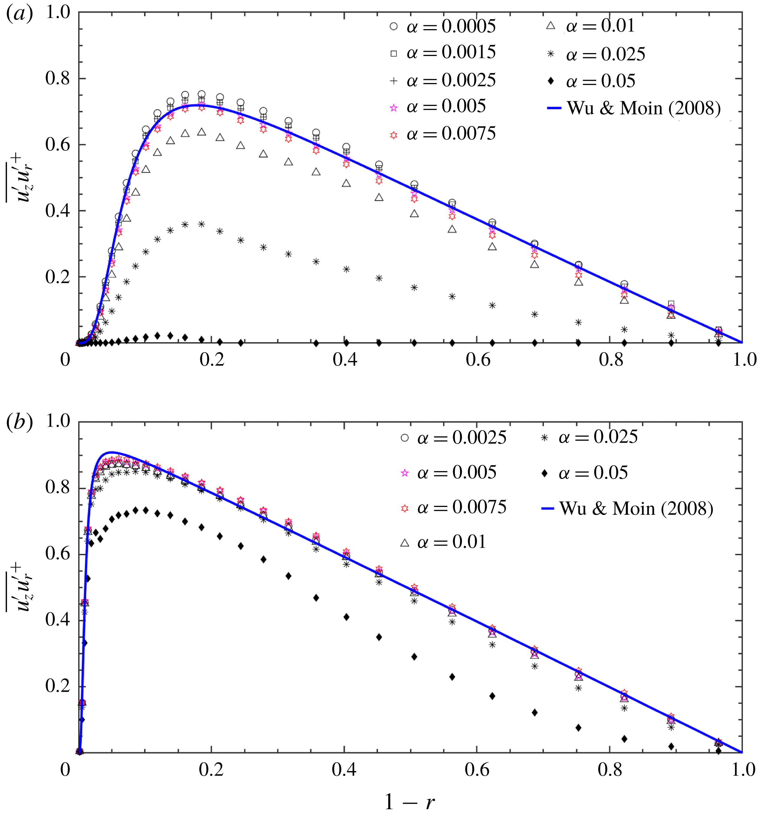
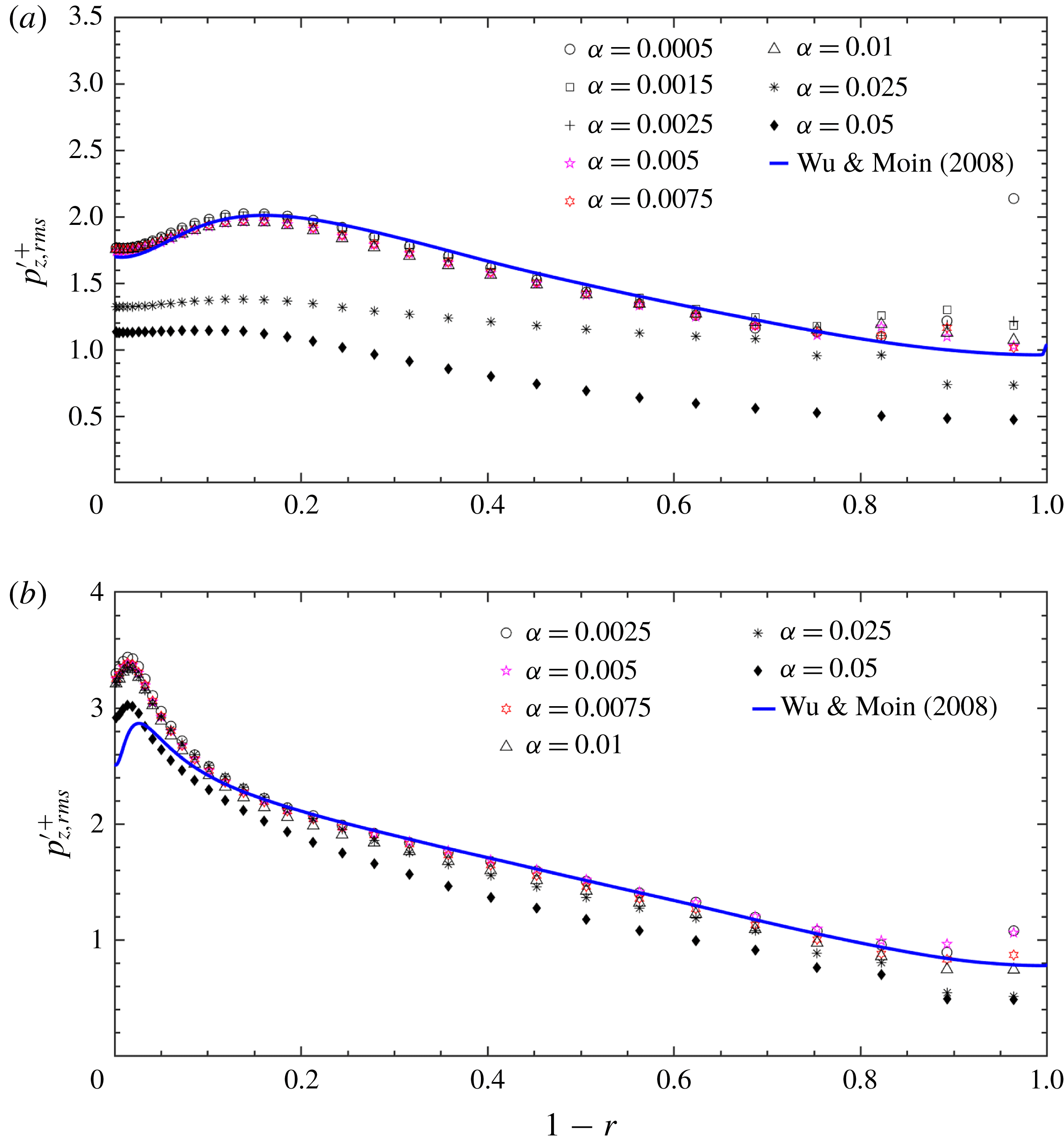
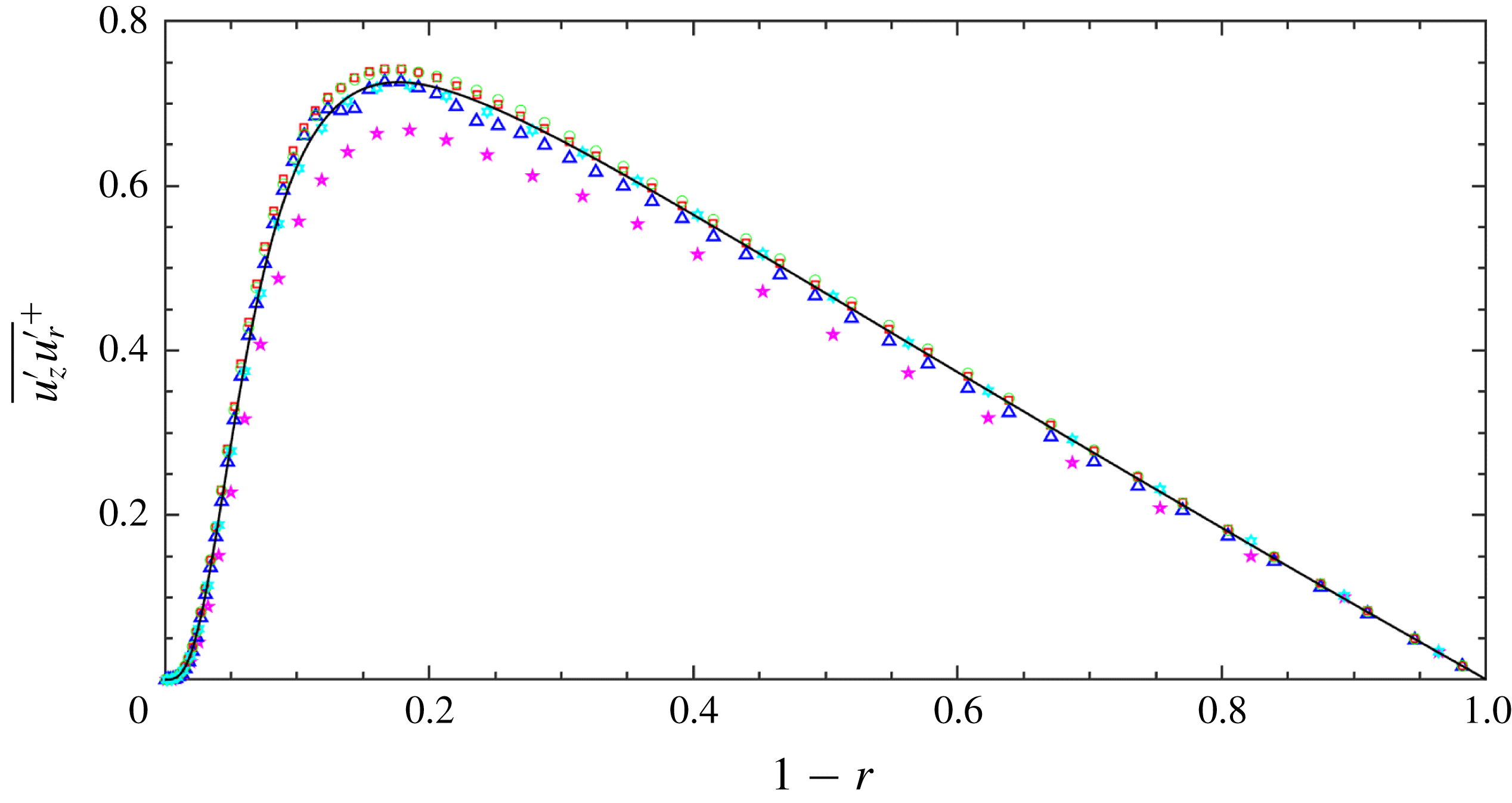
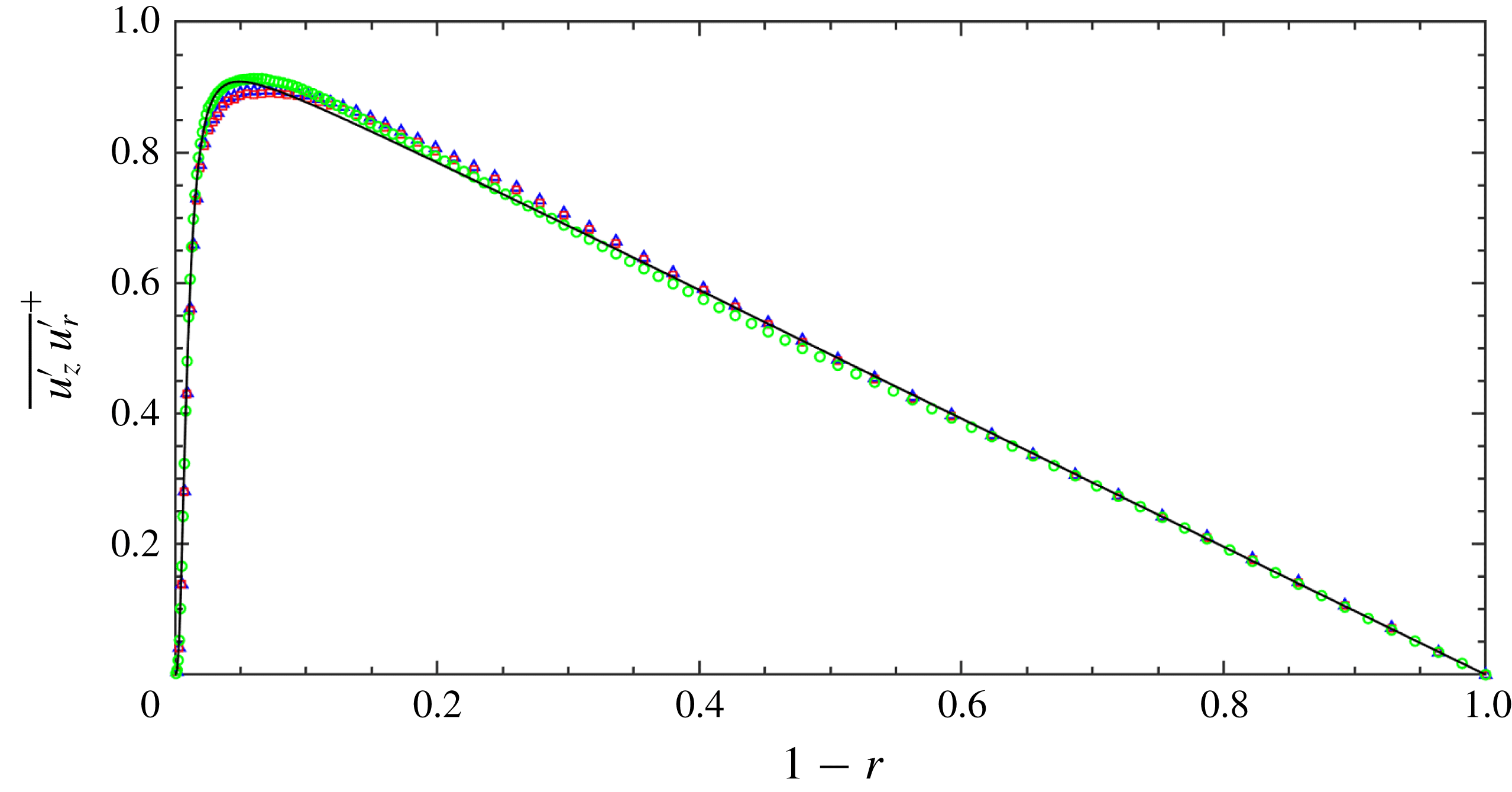
Figures 2–7 present the comparison of current mean and second-order statistics with the results from Wu & Moin (Reference Wu and Moin2008). In general, the EVM results agree with DNS quite well, although EVM simulations were carried out in Cartesian coordinates while the DNS of Wu & Moin (Reference Wu and Moin2008) was performed using cylindrical coordinates. From figure 2, we see that the agreement between the EVM mean velocities
 $\mathit{u}_{z}^{+}$
with those of DNS in Wu & Moin (Reference Wu and Moin2008) is excellent for both Reynolds numbers. Figures 3–7 compare the axial turbulence intensity
 $u_{z,rms}^{\prime +}$
, wall-normal turbulence intensity
 $u_{r,rms}^{\prime +}$
, azimuthal turbulence intensity
 $u_{\unicode[STIX]{x1D703},rms}^{\prime +}$
, turbulence shear stress
 $\overline{u_{z}^{\prime }u_{r}^{\prime }}^{+}$
and pressure fluctuations
 $p_{\mathit{rms}}^{\prime +}$
with their DNS counterparts in Wu & Moin (Reference Wu and Moin2008). At
 $Re_{D}=5300$
, the agreement is very good for all the results. At
 $Re_{D}=44\,000$
, however, the current EVM slightly overpredicts
 $u_{z,rms}^{\prime +}$
and
 $\overline{u_{z}^{\prime }u_{r}^{\prime }}^{+}$
in the region far away from the pipe wall. The agreement between EVM simulation and DNS in terms of
 $p_{\mathit{rms}}^{\prime +}$
is good in the region close to the pipe axis, however, the pressure fluctuation of EVM simulation is larger than that of DNS in the region close to the pipe wall. The agreement between EVM solutions of the other two components (azimuthal and radial) of turbulence intensities that are not shown in this paper from that of DNS are very similar to the statistics presented for
 $u_{z,rms}^{\prime +}$
.
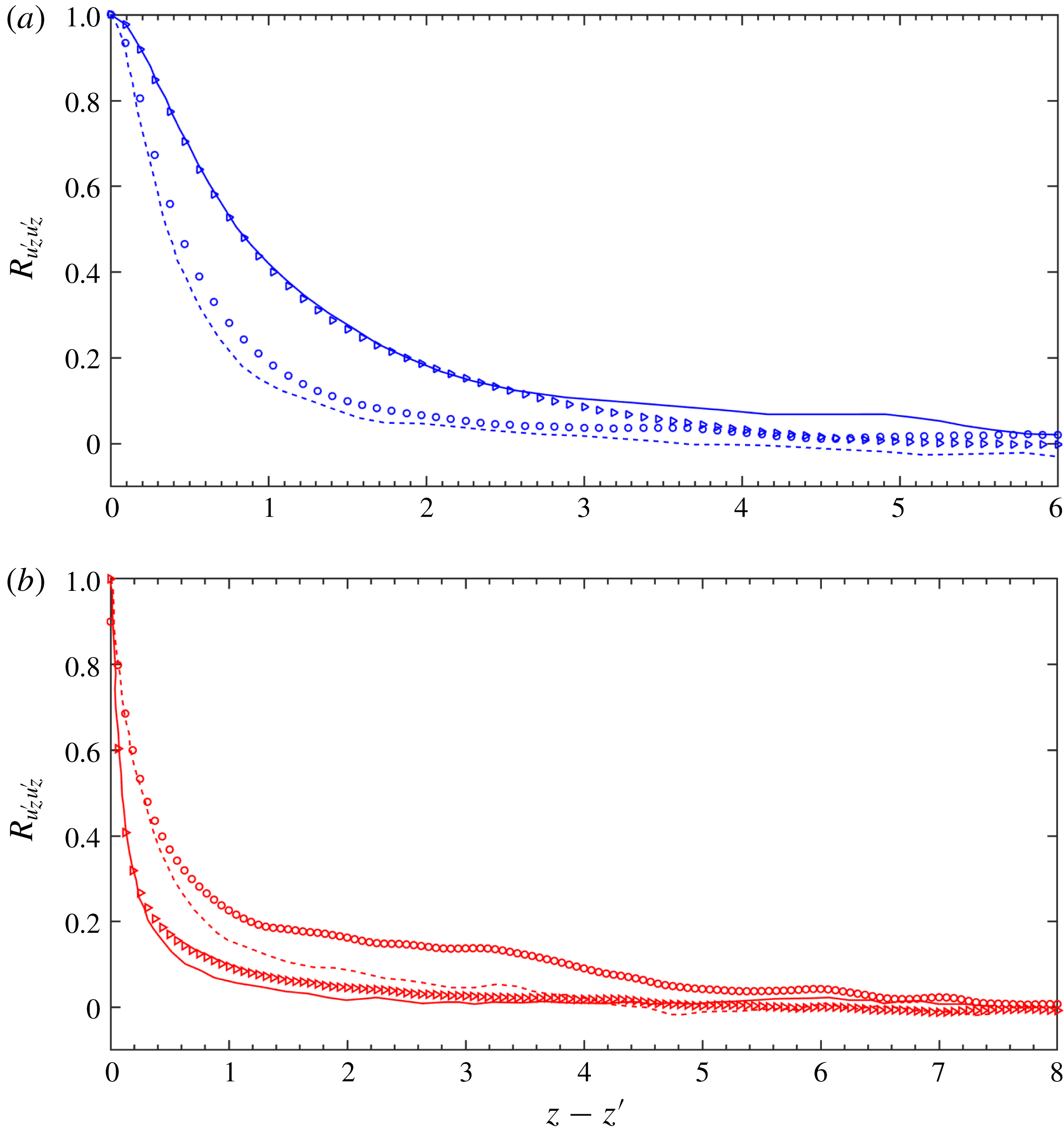
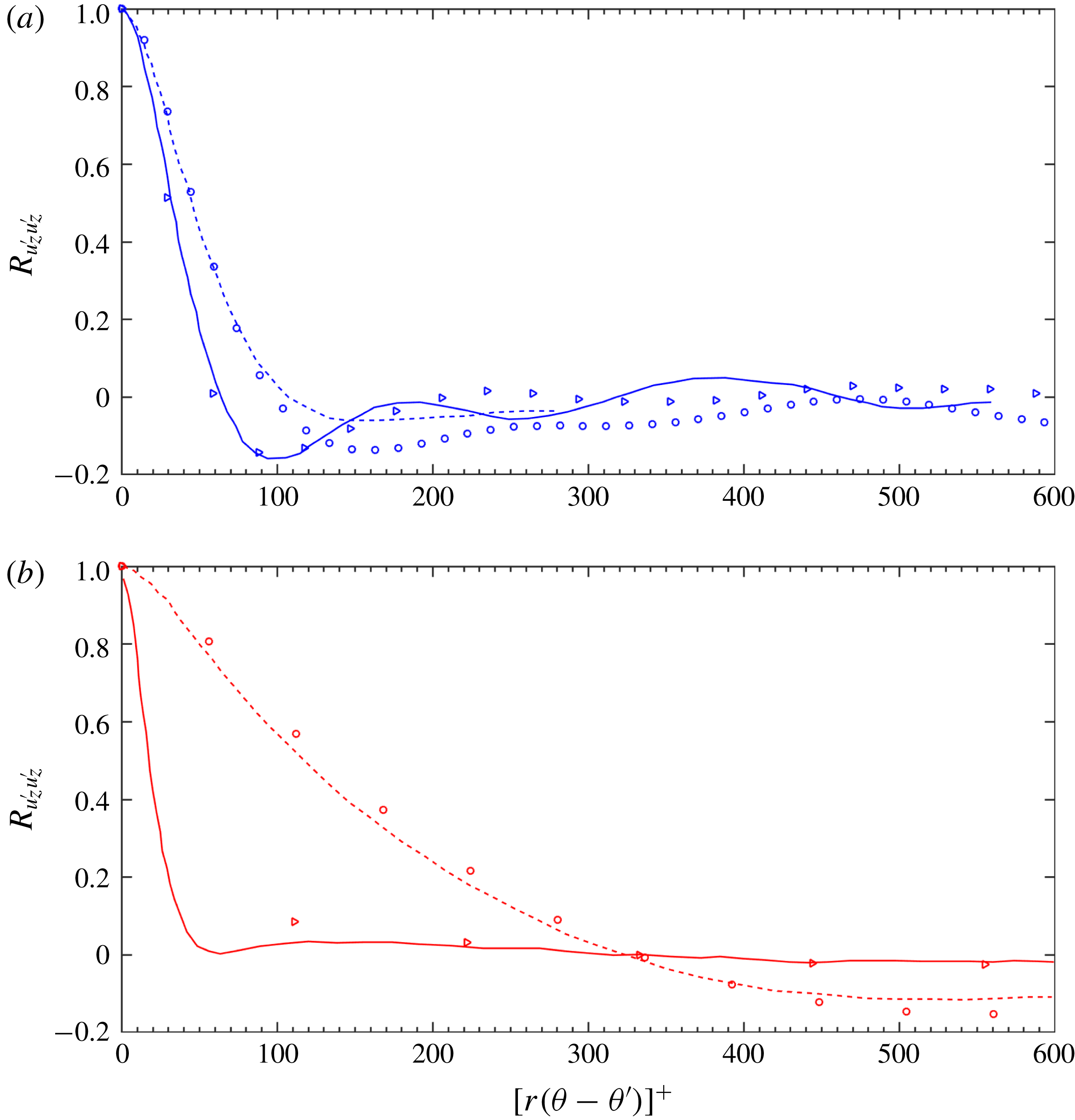
The comparisons of EVM simulations with DNS in terms of the two-point correlation coefficient
 $R_{u_{z}^{\prime }u_{z}^{\prime }}$
as a function of
 $z$
separation at two radial positions, namely
 $1-r=0.01$
and
 $1-r=0.5$
, are shown in figure 8. We see that the results are in reasonable agreement given the statistical uncertainty. We note that at lower
 $Re_{D}$
number, the correlation at position
 $(1-r)=0.01$
close to the wall is larger than that at
 $(1-r)=0.5$
. In contrast, at higher
 $Re_{D}$
the two-point correlation is smaller when the radial position is close to the wall. The EVM solution of
 $R_{u_{z}^{\prime }u_{z}^{\prime }}$
as a function of local azimuthal separation
 $[r(\unicode[STIX]{x1D703}-\unicode[STIX]{x1D703}^{\prime })]^{+}$
is compared with that of DNS in figure 9. Note that for clarity, similarly to Wu & Moin (Reference Wu and Moin2008), only the results with
 $[r(\unicode[STIX]{x1D703}-\unicode[STIX]{x1D703}^{\prime })]^{+}<600$
are presented. In figure 9(a), we see that at smaller
 $Re_{D}$
the agreement is quite good when
 $[r(\unicode[STIX]{x1D703}-\unicode[STIX]{x1D703}^{\prime })]^{+}<100$
. At larger
 $Re_{D}$
, as shown in figure 9(b), the agreement is excellent throughout
 $[r(\unicode[STIX]{x1D703}-\unicode[STIX]{x1D703}^{\prime })]^{+}<600$
.
Turbulent shear stress
 $\overline{u_{z}^{\prime }u_{r}^{\prime }}^{+}$
as a function of
 $(1-r)$
. For details see figure 2.

Intensity of pressure fluctuations
 $p_{\mathit{rms}}^{\prime +}$
as a function of
 $(1-r)$
. For details see figure 2.

Two-point correlation coefficient
 $R_{u_{z}^{\prime }u_{z}^{\prime }}$
as a function of the streamwise separation
 $z-z^{\prime }$
. (a) Blue solid line:
 $1-r=0.01$
, Wu & Moin (Reference Wu and Moin2008) at
 $Re_{D}=5300$
; blue dashed line:
 $1-r=0.5$
, Wu & Moin (Reference Wu and Moin2008) at
 $Re_{D}=5300$
; blue triangles:
 $1-r=0.01$
, present EVM at
 $Re_{D}=5300$
; blue circles:
 $1-r=0.5$
, present EVM at
 $Re_{D}=5300$
. (b) Red solid line:
 $1-r=0.01$
, Wu & Moin (Reference Wu and Moin2008) at
 $Re_{D}=44\,000$
; red dashed line:
 $1-r=0.5$
, Wu & Moin (Reference Wu and Moin2008) at
 $Re_{D}=44\,000$
; red triangles:
 $1-r=0.01$
, present EVM at
 $Re_{D}=44\,000$
; red circles:
 $1-r=0.5$
, present EVM at
 $Re_{D}=44\,000$
.

Two-point correlation coefficient
 $R_{u_{z}^{\prime }u_{z}^{\prime }}$
as a function of local azimuthal separation
 $[r(\unicode[STIX]{x1D703}-\unicode[STIX]{x1D703}^{\prime })]^{+}$
. For details see figure 8.

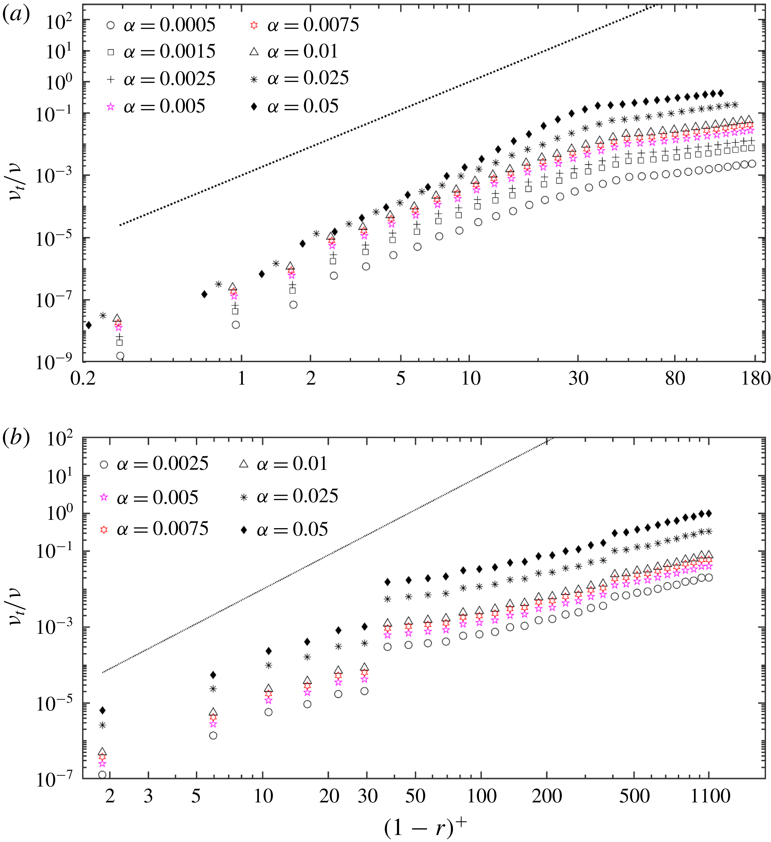
3.3 Near-wall scaling of EVM
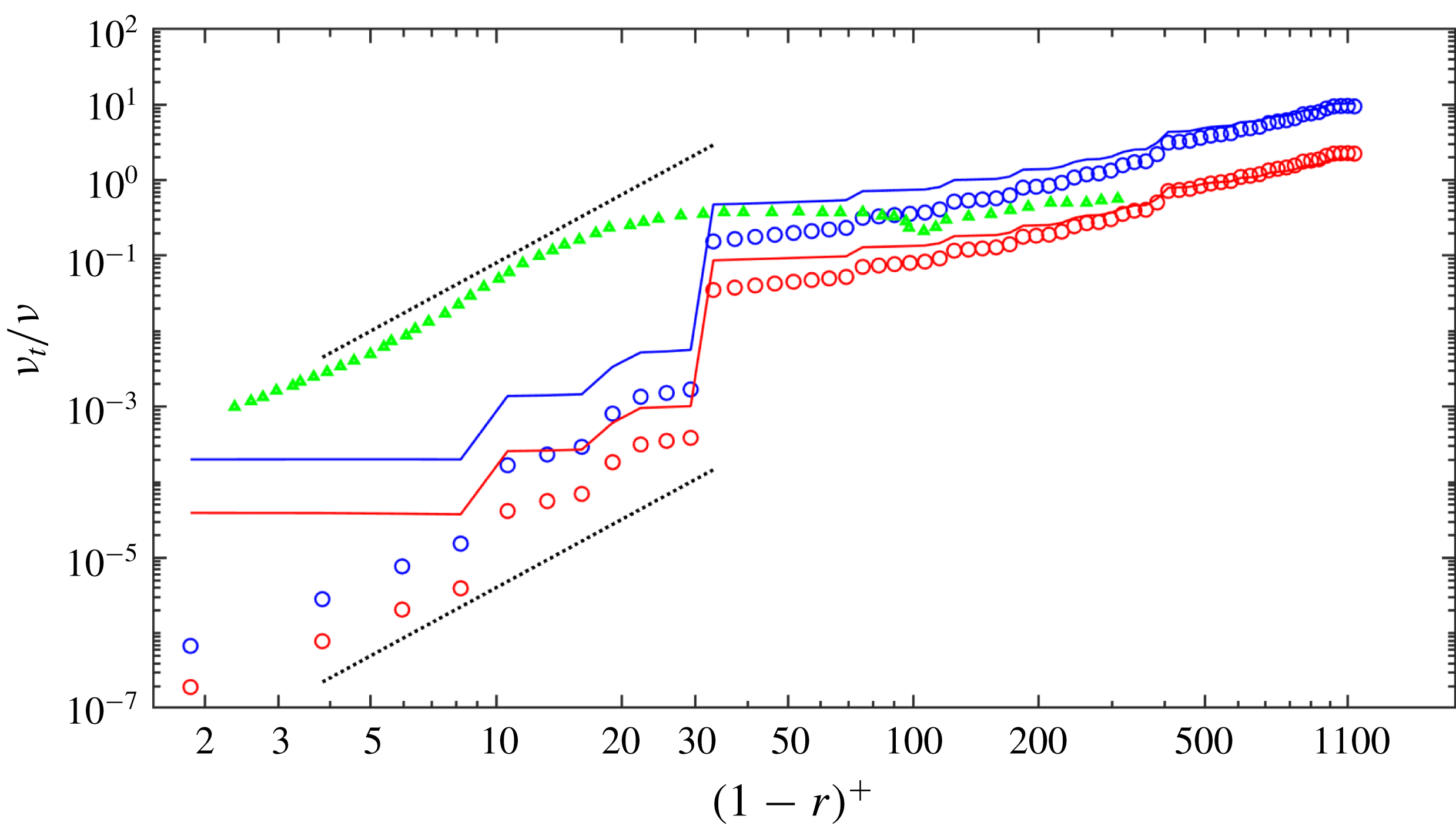
In order to assess the scaling of EVM near the wall
 $((1-r)^{+}<30)$
, where
 $\unicode[STIX]{x1D708}_{t}\propto O(1-r)^{3}$
(Nicoud & Ducros Reference Nicoud and Ducros1999), we have performed a posteriori tests for both Reynolds numbers at different resolutions. In the standard Smagorinsky model
 $\unicode[STIX]{x1D708}_{E}$
is not zero at the wall, although it is corrected in the Germano’s dynamic approach (Germano et al.
Reference Germano, Piomelli, Moin and Cabot1991). However, both models lead to erroneous scaling approaching the wall. In contrast, the eddy-viscosity model developed in Nicoud & Ducros (Reference Nicoud and Ducros1999) produces the cubic scaling with the distance from the wall. Here we present the results for the high Reynolds number
 $Re_{D}=44\,000$
and compare all three aforementioned models, in particular here we used the empirical van Driest damping factor for the Smagorinsky model at
 $(1-r)^{+}<5$
. We see in figure 10 that EVM follows the correct scaling and its value at the wall is two orders of magnitude lower compared to the corrected Smagorinsky model. Above
 $(1-r)^{+}>30$
, all three models behave similarly, hence also confirming the assumption in (2.6) that the numerical residual scales linearly the dissipation rate
 $\unicode[STIX]{x1D716}$
. We note that the WALE model of Nicoud & Ducros (Reference Nicoud and Ducros1999) was computed at a different Reynolds number (
 $Re_{D}=10\,000$
).
 $Re_{D}=44\,000$
. Comparison of the averaged entropy viscosity
 $\unicode[STIX]{x1D736}(\Vert R_{ijm}^{K}(\mathit{u})\Vert _{L^{\infty }(K)})/(\Vert E_{ijm}^{K}(\mathit{u})-\bar{E}(\mathit{u})\Vert _{L^{\infty }(\unicode[STIX]{x1D6FA})})\unicode[STIX]{x1D6FF}_{K}^{2}$
with the eddy viscosity of the Smagorinsky model
 $(C_{s}\unicode[STIX]{x1D6FF}_{K})^{2}\overline{\unicode[STIX]{x1D64E}}$
for different resolutions. Both entropy viscosity and eddy viscosity are normalized by the physical viscosity. Blue colour corresponds to low resolution (
 $M=5$
) and red colour to high resolution (
 $M=8$
). Symbols denote the results of the entropy-viscosity model while solid lines denote the results of the eddy-viscosity model. The green triangles correspond to the eddy viscosity using the WALE model at
 $Re_{D}=10\,000$
(Nicoud & Ducros Reference Nicoud and Ducros1999). The two black dotted lines both show the scaling
 $\unicode[STIX]{x1D708}_{t}=O((1-r)^{3})$
. We have employed
 $\unicode[STIX]{x1D6FC}=0.005$
for EVM and
 $C_{s}=0.17$
for the Smagorinsky model (corresponding to the blue and red solid lines).

4 Vibrating pipe
In this section, we will investigate the effect of a periodic pipe motion on fully developed turbulent flow. We employ a coordinate transformation (stretching the
 $z$
-direction) to take the boundary deformation into account as first proposed in the work of Newman & Karniadakis (Reference Newman and Karniadakis1997), where the transformation-related terms appear as acceleration forces in the Navier–Stokes equations.
For the simulations in this section, the bulk velocity was also fixed as
 $\mathit{u}_{\mathit{bulk}}=1$
, which makes the Reynolds number
 $Re_{D}=5300$
. The length of the pipe is extended to
 $12D$
, thus to maintain the same resolution as that of the stationary pipe, the number of Fourier planes is increased to 256 along the
 $z$
direction, and we use fourth-order Jacobi polynomial as before.
The pipe is forced to vibrate under a standing-wave pattern in both
 $x$
and
 $y$
direction. The displacement in the
 $y$
-direction is as follows:
 $$\begin{eqnarray}d_{y}=A\cos \left(2n\unicode[STIX]{x03C0}{\displaystyle \frac{z}{L}}+\unicode[STIX]{x1D719}_{z}\right)\cdot \cos (2\unicode[STIX]{x03C0}ft+\unicode[STIX]{x1D719}_{t}),\end{eqnarray}$$
where
 $L=12D$
is the pipe length,
 $A$
is the amplitude of the standing wave,
 $\unicode[STIX]{x1D719}_{z}$
and
 $\unicode[STIX]{x1D719}_{t}$
are phase differences:
 $\unicode[STIX]{x1D719}_{z}=0.5\unicode[STIX]{x03C0}$
in both the
 $x$
and
 $y$
direction, which forces zero displacements at the ends of the pipe (nodes);
 $\unicode[STIX]{x1D719}_{t}=0$
in
 $x$
direction and
 $\unicode[STIX]{x1D719}_{t}=0.5\unicode[STIX]{x03C0}$
in the
 $y$
direction. We also set
 $n=4$
, hence there are four waves along the pipe with a wavelength
 $\unicode[STIX]{x1D706}=3D$
;
 $f=0.078$
is the corresponding frequency. The values of
 $n$
and
 $f$
are chosen based on the results of our studies of laminar flow-induced vibration in Xie et al. (Reference Xie, Zheng, Triantafyllou, Constantinides and Karniadakis2016), and turbulent flow-induced free vibration (not presented in this paper). In these studies, we found that the fourth mode vibration with
 $f=0.078$
was the most readily excited.
We have systematically simulated 11 cases in total with the wave steepness
 $s_{o}=2A/\unicode[STIX]{x1D706}$
increasing from 0 to 0.0667 (
 $A=0.1D$
). All the simulations were performed over
 $350D/\overline{\boldsymbol{u}}_{\mathit{bulk}}$
time units and the statistical quantities were collected in a time duration of
 $250D/\overline{\boldsymbol{u}}_{\mathit{bulk}}$
, which is approximately 20 periods of the standing wave, sufficient for obtaining a statistically steady value.
Before discussing the results, it is important to clarify the following three points:
(i) Hereafter, all the mean values and fluctuations are converted into wall units, based on the friction velocity of each case.
(ii) The total velocity can be decomposed into two parts as follows,
(4.2)where $$\begin{eqnarray}\mathit{u}_{\mathit{total}}=\mathit{u}_{\mathit{relative}}+\mathit{u}_{\mathit{pipe}},\end{eqnarray}$$
$\mathit{u}_{\mathit{pipe}}$
is the velocity of the pipe subject to a standing-wave motion: when
$\mathit{u}_{\mathit{pipe}}$
dominates the total velocity
$\mathit{u}_{\mathit{total}}$
, some highly useful information might be hidden if the statistics are taken from
$\mathit{u}_{\mathit{total}}$
. Therefore, in this section we only analyse the relative velocity
$\mathit{u}_{\mathit{relative}}$
, which is the solution of the Navier–Stokes equations (2.2).
(iii) Different from the whole averaging of a stationary pipe, for the vibrating pipe, the statistics are obtained separately at pipe nodes and anti-nodes. For the quantity of interest, e.g.
$\unicode[STIX]{x1D719}$
, at a streamwise position
$z_{K}$
, either be a node or anti-node, at time instant
$t_{n}$
, when the anti-nodes reach their maximum displacement, the phase-averaged mean and fluctuations are computed as follows, (4.3)$$\begin{eqnarray}\displaystyle & \displaystyle \overline{\unicode[STIX]{x1D719}}(r,z_{K})={\displaystyle \frac{1}{N_{t}N_{\unicode[STIX]{x1D703}}}}\mathop{\sum }_{n=1}^{N_{t}}\mathop{\sum }_{i=1}^{N_{\unicode[STIX]{x1D703}}}\unicode[STIX]{x1D719}(t_{n},r,\unicode[STIX]{x1D703}_{i},z_{K}), & \displaystyle\end{eqnarray}$$
(4.4)where$$\begin{eqnarray}\displaystyle & \displaystyle \unicode[STIX]{x1D719}_{\mathit{rms}}^{\prime }(r,z_{K})=\left[{\displaystyle \frac{1}{N_{t}N_{\unicode[STIX]{x1D703}}}}\mathop{\sum }_{n=1}^{N_{t}}\mathop{\sum }_{i=1}^{N_{\unicode[STIX]{x1D703}}}\unicode[STIX]{x1D719}^{2}(t_{n},r,\unicode[STIX]{x1D703}_{i},z_{K})-\overline{\unicode[STIX]{x1D719}}^{2}(r,z_{K})\right]^{1/2}, & \displaystyle\end{eqnarray}$$
$N_{t}$
is the number of time instants for the phase averaging,
$N_{\unicode[STIX]{x1D703}}$
is the number of sampling points and
$\unicode[STIX]{x1D703}_{i}$
is the
$i$
th point in the azimuthal direction. Specifically, according to the definition above, we start the simulation from a state that the anti-nodes are at their maximum displacement, and perform the phase averaging every 6410 time steps, i.e. a time interval of
$\unicode[STIX]{x0394}t=6.41D/\overline{\mathit{u}}_{\mathit{bulk}}$
, which is equal to the half-period of the prescribed standing-wave motion that has a frequency
$f=0.078$
.




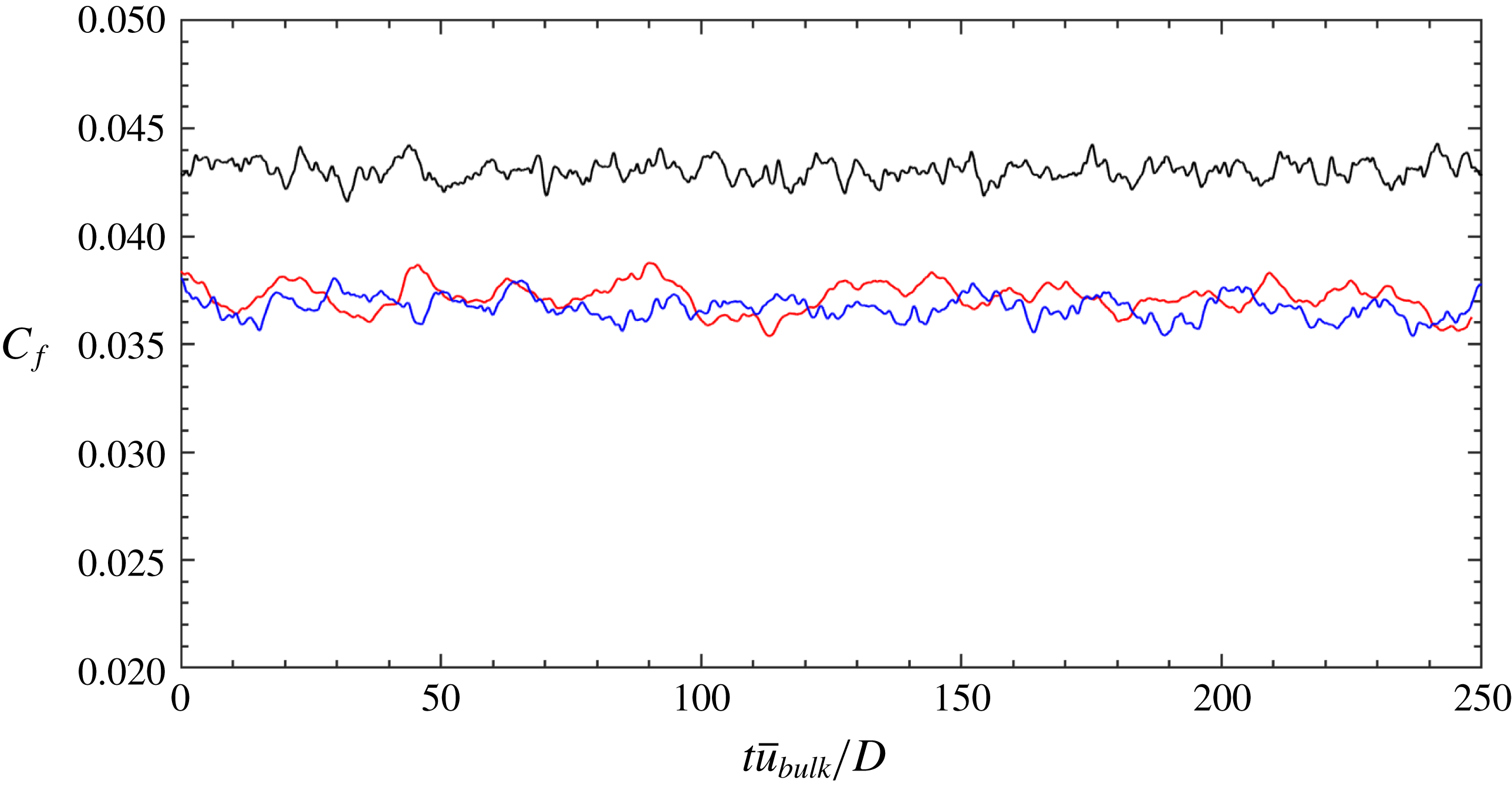
Time history of friction factor
 $C_{f}$
at different values of wave steepness
 $s_{o}=2A/\unicode[STIX]{x1D706}$
. Red line: stationary pipe; blue line:
 $s_{o}=0.013$
; black line:
 $s_{o}=0.067$
. Note that
 $t$
has been shifted to start from zero.

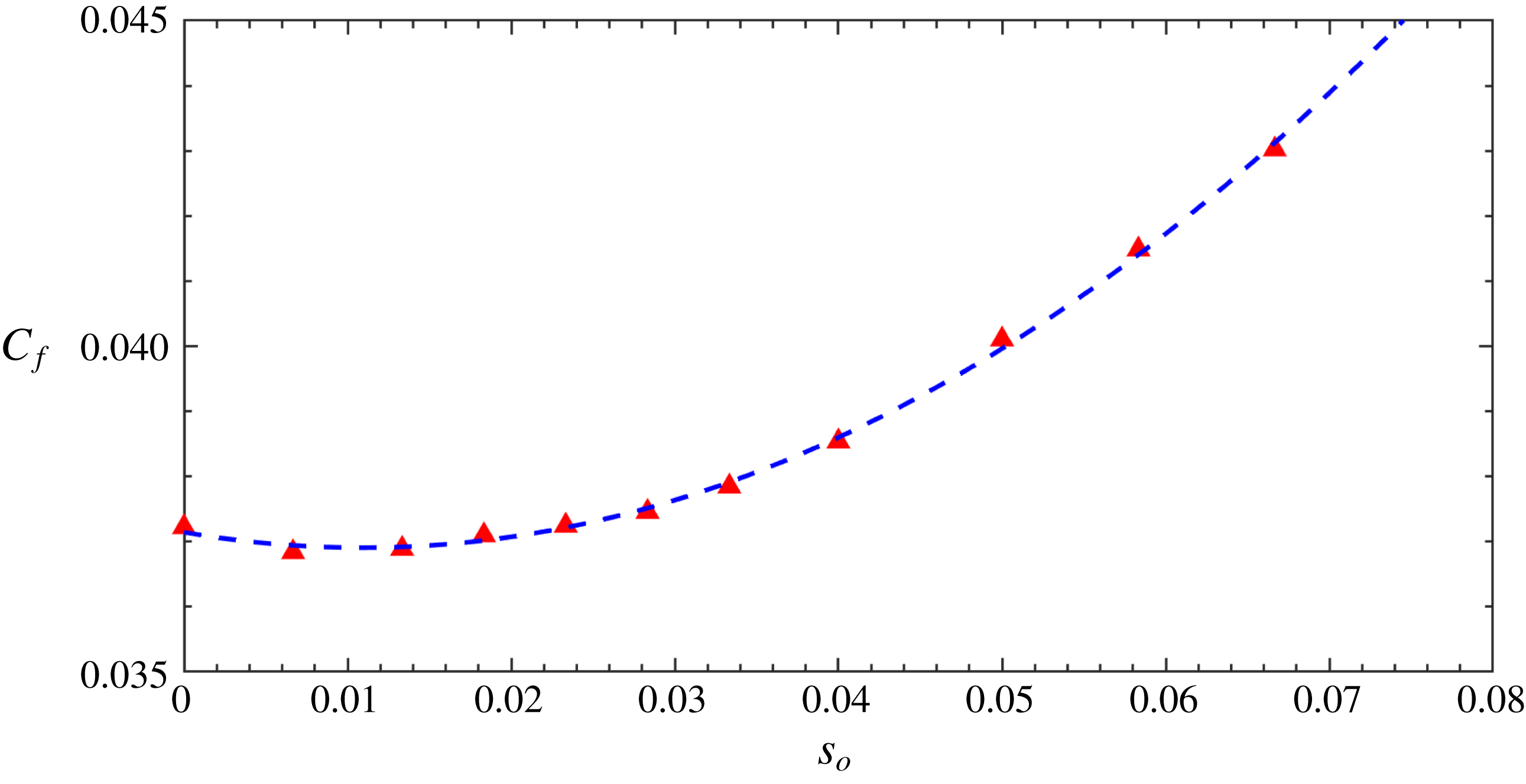
Friction factor
 $C_{f}$
as a function of wave steepness
 $s_{o}$
. The blue dashed line is a quadratic fitting by using the formula
 $C_{f}=2.054s_{o}^{2}-0.0463s_{o}+0.0371$
.

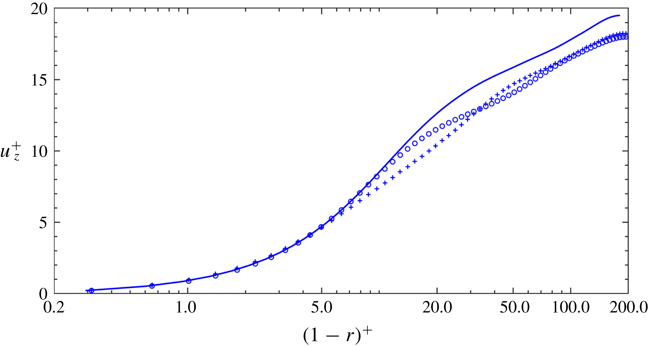
Mean axial velocity
 $u_{z}^{+}$
as a function
 $(1-r)^{+}$
. Solid line: stationary pipe,
 $s_{o}=0$
; plus signs: node average,
 $s_{o}=0.0667$
; circles: anti-node average,
 $s_{o}=0.0667$
.

Figure 11 shows the time variation of friction factor
 $C_{f}=8(u_{\unicode[STIX]{x1D70F}}^{2}/\overline{u}_{\mathit{bulk}}^{2})$
at different
 $s_{o}$
during the time interval
 $\unicode[STIX]{x0394}t=250D/\overline{\mathit{u}}_{\mathit{bulk}}$
. As expected, for turbulent pipe flow,
 $C_{f}$
exhibits fluctuations with time but a statistically stationary state has been achieved. Note that the fluctuations of wall shear stress reveals the fact that the mean velocity at the wall is changing with time, and this is also presented in Keirsbulck, Labraga & el Hak (Reference Keirsbulck, Labraga and el Hak2012) for plane channel flow. Figure 12 shows the friction factor
 $C_{f}$
from all of the 11 simulations with respect to the variation of
 $s_{o}$
. Also shown in this figure is a quadratic fitting curve
 $C_{f}=2.054s_{o}^{2}-0.0463s_{o}+0.0371$
, which seems to be the correct functional relationship. Some small drag reduction is evident for small pipe vibrations around
 $s_{o}\approx 0.01$
.
4.1 Mean flow
First of all, we would like to note that in this section, the turbulence quantities are normalized by the corresponding friction velocity, i.e.
 $u_{\unicode[STIX]{x1D70F}}=0.0683\overline{\mathit{u}}_{\mathit{bulk}}$
for the stationary pipe and
 $u_{\unicode[STIX]{x1D70F}}=0.0733\overline{\mathit{u}}_{\mathit{bulk}}$
for the case of
 $s_{o}=0.0667$
. In figure 13, it can be observed that when the pipe is vibrating, both at the node and anti-node the mean axial velocity in wall units changes notably. In the region of
 $5<(1-r)^{+}<34$
, the value of
 $\overline{u}_{z}^{+}$
at an anti-node exceeds that at a node, while the opposite is true in the region of
 $(1-r)^{+}>34$
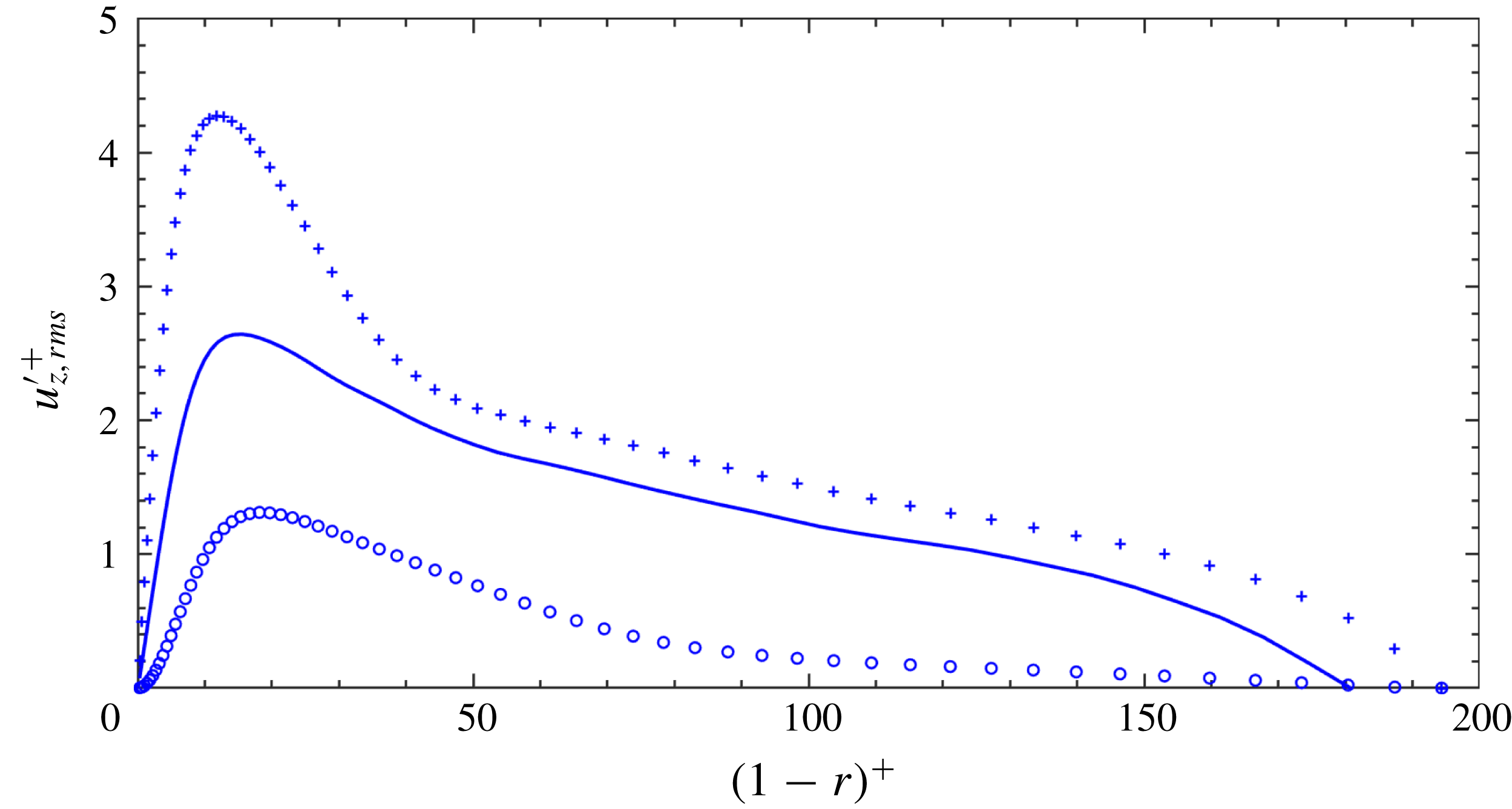
. The comparison of streamwise fluctuations
 $u_{z,rms}^{\prime +}$
is presented in figure 14. The magnitude of phase averaged
 $u_{z,rms}^{\prime +}$
of a stationary pipe is between that at a node and anti-node, while the magnitude at a node is larger than that at an anti-node substantially over the entire region of
 $(1-r)^{+}$
. In addition, the radial position where
 $u_{z,rms}^{\prime +}$
at the anti-nodes reaches a peak is shifted farther away from the pipe wall compared with that at the nodes. We also note that in figure 14,
 $u_{z,rms}^{\prime +}$
is approaching zero near the pipe axis, which is different from the distribution in figure 3. The difference is due to the way that we perform the averaging. As shown in (3.1), here averaging is employed along the azimuthal direction only, but at the pipe axis, the value of
 $u$
is unique, thus
 $u$
is constant azimuthally.
Axial turbulence intensity
 $u_{z,rms}^{\prime +}$
as a function of
 $(1-r)^{+}$
. For details see figure 13.

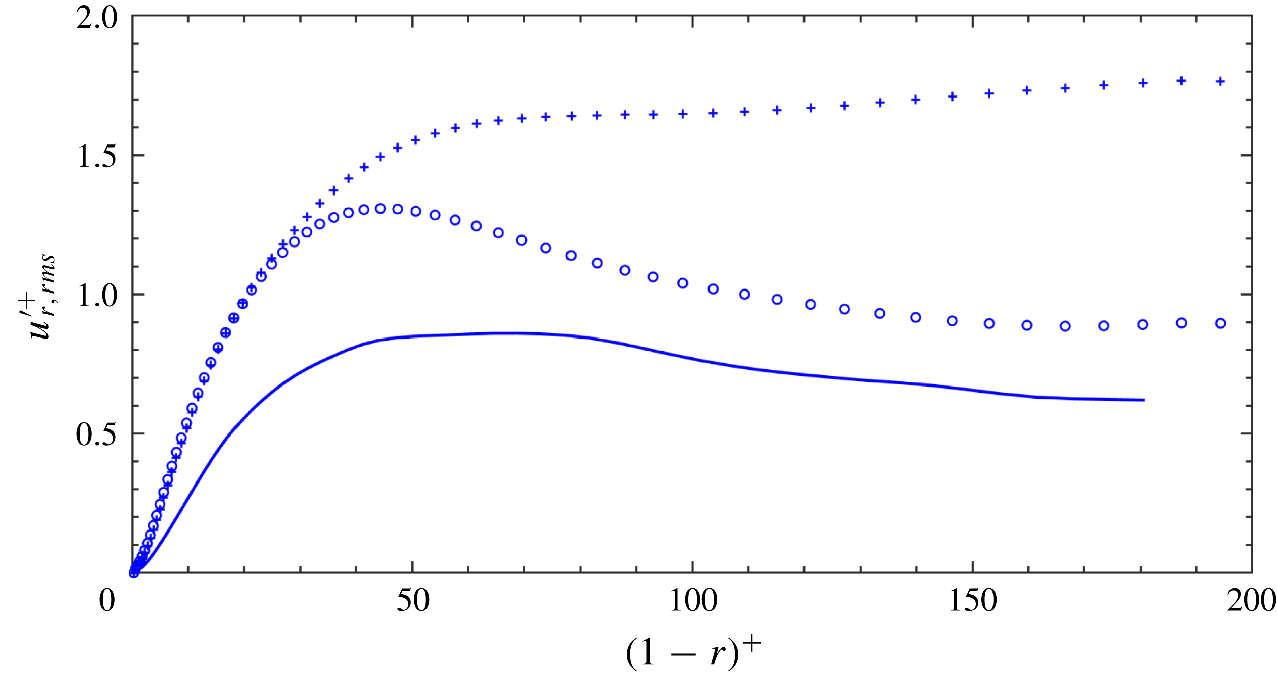
Wall-normal turbulence intensity
 $u_{r,rms}^{\prime +}$
as a function
 $(1-r)^{+}$
. For details see figure 13.

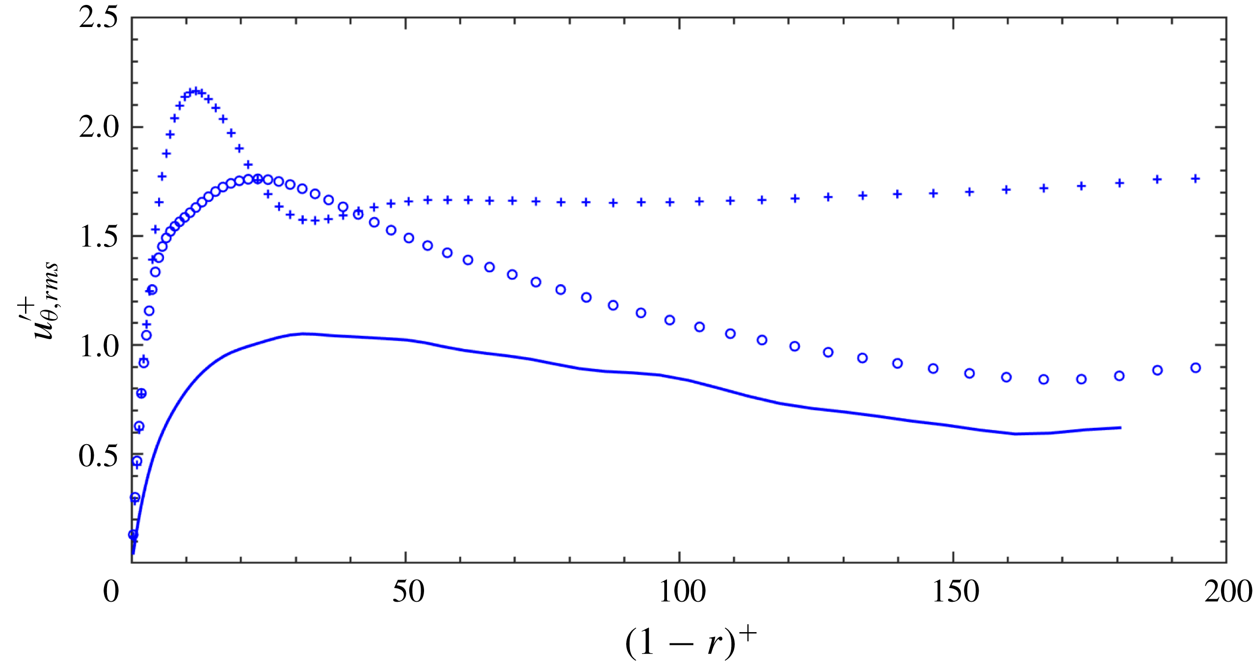
Azimuthal turbulence intensity
 $u_{\unicode[STIX]{x1D703},rms}^{\prime +}$
as a function
 $(1-r)^{+}$
. For details see figure 13.

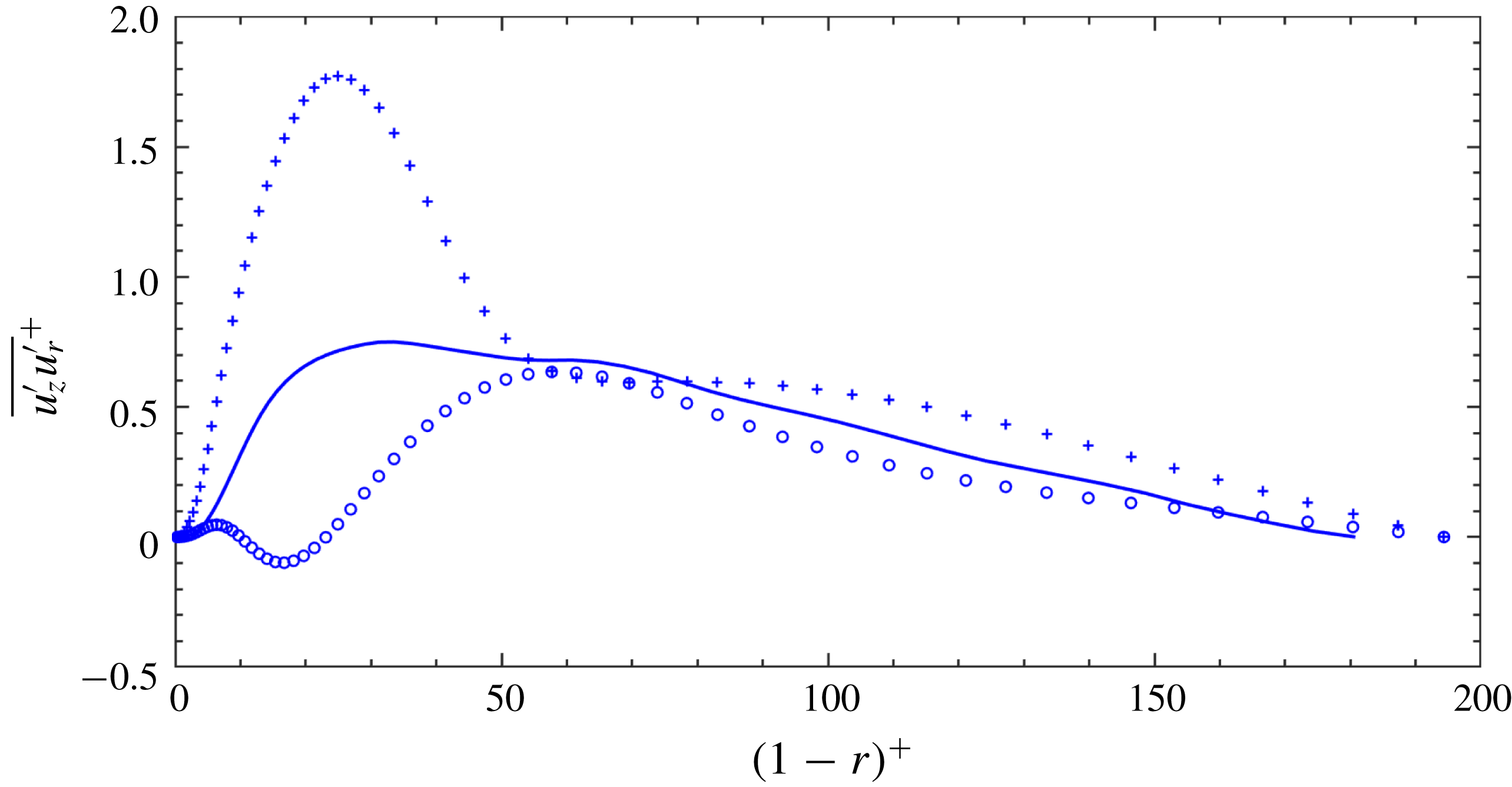
Turbulent shear stress
 $\overline{u_{z}^{\prime }u_{r}^{\prime }}^{+}$
as a function
 $(1-r)^{+}$
. For details see figure 13.

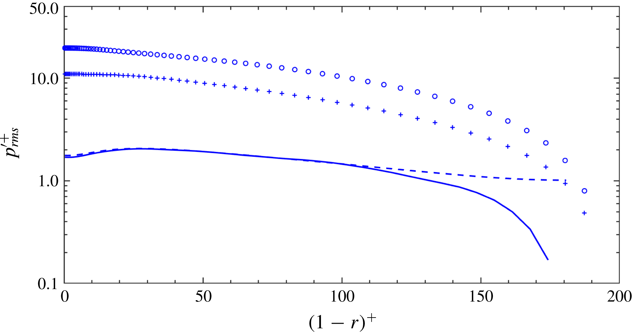
Intensity of the pressure fluctuation
 $p_{\mathit{rms}}^{\prime +}$
as a function of
 $(1-r)^{+}$
. Solid line: sectional average (20 snapshots), stationary pipe,
 $s_{o}=0$
; plus signs: node average,
 $s_{o}=0.0667$
; circles: anti-node average,
 $s_{o}=0.0667$
; dashed line: whole average, stationary pipe.

In figure 15, the radial turbulence fluctuations (
 $u_{r,rms}^{\prime +}$
) of the vibrating pipe both at the nodes and anti-nodes are significantly larger than those of a stationary pipe. This is the same for the distribution of
 $u_{z,rms}^{\prime +}$
, the values of
 $u_{r,rms}^{\prime +}$
at a node surpass those at an anti-node in the region of
 $(1-r)^{+}>23$
. The distribution of the azimuthal component of turbulence fluctuations (
 $u_{\unicode[STIX]{x1D703},rms}^{\prime +}$
) is shown in figure 16; interestingly, it can be observed that, only in the region of
 $23<(1-r)^{+}<41$
, the values of
 $u_{\unicode[STIX]{x1D703},rms}^{\prime +}$
at an anti-node are larger than those at a node. For the turbulent shear stress
 $\overline{u_{z}^{\prime }u_{r}^{\prime }}^{+}$
, the impact of vibration is also very prominent, as shown in figure 17: firstly, the linear distribution of the shear stress no longer exists; secondly, the value of
 $\overline{u_{z}^{\prime }u_{r}^{\prime }}^{+}$
is changed substantially compared with that of a stationary pipe; thirdly,
 $\overline{u_{z}^{\prime }u_{r}^{\prime }}^{+}$
at an anti-node has a negative value in the region of
 $10<(1-r)^{+}<23$
.
Figure 18 compares the intensity of the pressure fluctuations
 $p_{\mathit{rms}}^{\prime +}$
. It can be seen that the pressure fluctuations change substantially when the pipe is vibrating. Different from the velocity fluctuations, over the entire radial distance, the pressure fluctuations at an anti-node are much larger than those at a node. Note that, in this figure, the magnitude of the pressure fluctuation of a stationary pipe based on sectional averaging (solid line) at the axis is smaller than that corresponding to the whole averaging (dashed line).
Taking the divergence of the momentum equation (2.2) yields the following Poisson equation for pressure,
 $$\begin{eqnarray}\unicode[STIX]{x1D6FB}^{2}p=\unicode[STIX]{x1D735}\boldsymbol{\cdot }(\mathit{u}\boldsymbol{\cdot }\unicode[STIX]{x1D735}\mathit{u})+\unicode[STIX]{x1D735}\boldsymbol{\cdot }\mathit{F}.\end{eqnarray}$$
Here
 $F$
is the acceleration due to pipe motion, the detailed form of which could be found in Newman & Karniadakis (Reference Newman and Karniadakis1997). Unlike the pressure equation in Kim (Reference Kim1989), here the extra second term (
 $\unicode[STIX]{x1D735}\boldsymbol{\cdot }\mathit{F}$
) on the right-hand side of the above equation is due to pipe vibration that generates extra pressure fluctuations. Specifically, in cylindrical coordinates,
 $\unicode[STIX]{x1D735}\boldsymbol{\cdot }\mathit{F}$
can be expanded as follows,
 $$\begin{eqnarray}\left.\begin{array}{@{}c@{}}\unicode[STIX]{x1D735}\boldsymbol{\cdot }\mathit{F}=\left\{{\displaystyle \frac{\unicode[STIX]{x2202}^{2}u_{z}}{\unicode[STIX]{x2202}t\unicode[STIX]{x2202}r}}{\displaystyle \frac{\unicode[STIX]{x2202}\unicode[STIX]{x1D709}_{r}}{\unicode[STIX]{x2202}z}}+{\displaystyle \frac{1}{r}}{\displaystyle \frac{\unicode[STIX]{x2202}^{2}u_{z}}{\unicode[STIX]{x2202}t\unicode[STIX]{x2202}\unicode[STIX]{x1D703}}}{\displaystyle \frac{\unicode[STIX]{x2202}\unicode[STIX]{x1D709}_{\unicode[STIX]{x1D703}}}{\unicode[STIX]{x2202}z}}\right\}+2\left\{{\displaystyle \frac{\unicode[STIX]{x2202}u_{z}}{\unicode[STIX]{x2202}r}}{\displaystyle \frac{\unicode[STIX]{x2202}^{2}\unicode[STIX]{x1D709}_{r}}{\unicode[STIX]{x2202}t\unicode[STIX]{x2202}z}}+{\displaystyle \frac{1}{r}}{\displaystyle \frac{\unicode[STIX]{x2202}u_{z}}{\unicode[STIX]{x2202}\unicode[STIX]{x1D703}}}{\displaystyle \frac{\unicode[STIX]{x2202}^{2}\unicode[STIX]{x1D709}_{\unicode[STIX]{x1D703}}}{\unicode[STIX]{x2202}t\unicode[STIX]{x2202}z}}\right\}\\ +\left\{{\displaystyle \frac{\unicode[STIX]{x2202}(\mathit{u}\boldsymbol{\cdot }\unicode[STIX]{x1D735}u_{z})}{\unicode[STIX]{x2202}r}}{\displaystyle \frac{\unicode[STIX]{x2202}\unicode[STIX]{x1D709}_{r}}{\unicode[STIX]{x2202}z}}+{\displaystyle \frac{1}{r}}{\displaystyle \frac{\unicode[STIX]{x2202}(\mathit{u}\boldsymbol{\cdot }\unicode[STIX]{x1D735}u_{z})}{\unicode[STIX]{x2202}\unicode[STIX]{x1D703}}}{\displaystyle \frac{\unicode[STIX]{x2202}\unicode[STIX]{x1D709}_{\unicode[STIX]{x1D703}}}{\unicode[STIX]{x2202}z}}\right\}+2u_{z}\left\{{\displaystyle \frac{\unicode[STIX]{x2202}u_{z}}{\unicode[STIX]{x2202}r}}{\displaystyle \frac{\unicode[STIX]{x2202}^{2}\unicode[STIX]{x1D709}_{r}}{\unicode[STIX]{x2202}z^{2}}}+{\displaystyle \frac{1}{r}}{\displaystyle \frac{\unicode[STIX]{x2202}u_{z}}{\unicode[STIX]{x2202}\unicode[STIX]{x1D703}}}{\displaystyle \frac{\unicode[STIX]{x2202}^{2}\unicode[STIX]{x1D709}_{\unicode[STIX]{x1D703}}}{\unicode[STIX]{x2202}z^{2}}}\right\}\\ +2u_{z}\left\{{\displaystyle \frac{\unicode[STIX]{x2202}p}{\unicode[STIX]{x2202}r}}{\displaystyle \frac{\unicode[STIX]{x2202}^{2}\unicode[STIX]{x1D709}_{r}}{\unicode[STIX]{x2202}z^{2}}}+{\displaystyle \frac{1}{r}}{\displaystyle \frac{\unicode[STIX]{x2202}p}{\unicode[STIX]{x2202}\unicode[STIX]{x1D703}}}{\displaystyle \frac{\unicode[STIX]{x2202}^{2}\unicode[STIX]{x1D709}_{\unicode[STIX]{x1D703}}}{\unicode[STIX]{x2202}z^{2}}}\right\}+\left\{{\displaystyle \frac{\unicode[STIX]{x2202}^{2}p}{\unicode[STIX]{x2202}r\unicode[STIX]{x2202}z}}{\displaystyle \frac{\unicode[STIX]{x2202}\unicode[STIX]{x1D709}_{r}}{\unicode[STIX]{x2202}z}}+{\displaystyle \frac{1}{r}}{\displaystyle \frac{\unicode[STIX]{x2202}^{2}p}{\unicode[STIX]{x2202}\unicode[STIX]{x1D703}\unicode[STIX]{x2202}z}}{\displaystyle \frac{\unicode[STIX]{x2202}\unicode[STIX]{x1D709}_{\unicode[STIX]{x1D703}}}{\unicode[STIX]{x2202}z}}\right\},\end{array}\right\}\end{eqnarray}$$
where
 $(\unicode[STIX]{x1D709}_{r},\unicode[STIX]{x1D709}_{\unicode[STIX]{x1D703}})$
is the pipe displacement vector in cylindrical coordinates. In (4.6), the last two terms within
 $\{\}$
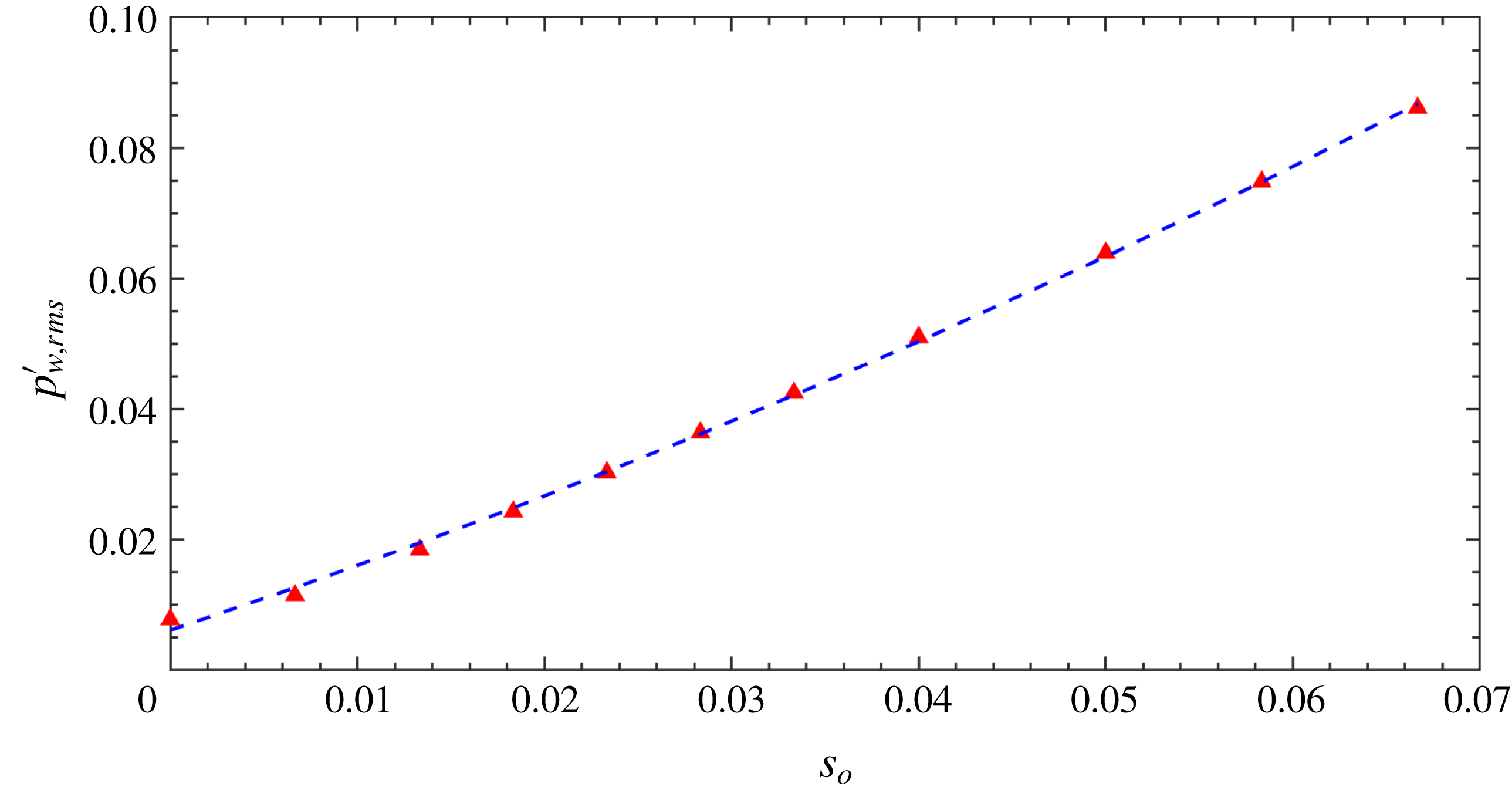
play a role in redistributing the pressure fluctuations to the entire pipe domain. It is rather complicated to derive analytically the dependence of the pressure fluctuations on the pipe vibration amplitude, however, we can fit the simulation data. We obtain a quadratic dependence as shown in figure 19, which exhibits the wall pressure fluctuations
 $p_{\mathit{w,\, rms}}^{\prime }$
from the 11 simulations with respect to
 $s_{o}$
, as well as a quadratic fitting curve
 $p_{\mathit{w,\, rms}}^{\prime }=3.873s_{o}^{2}+0.95s_{o}+0.006$
.
In conclusion, from the phase-averaged statistics, we can observe that the intensity of the axial velocity fluctuations decreases at anti-nodes but increases at nodes; the intensity of the other two velocity components increases both at nodes and anti-nodes. The intensity of the pressure fluctuations increases substantially both at nodes and anti-nodes due to pipe vibration.
Wall pressure fluctuations
 $p_{\mathit{w,\,rms}}^{\prime }$
as a function of wave steepness
 $s_{o}$
. The blue dashed line is a quadratic fitting by using the formula
 $p_{\mathit{w,\, rms}}^{\prime }=3.873s_{o}^{2}+0.95s_{o}+0.006$
. Note here
 $p_{\mathit{w,\,rms}}^{\prime }$
is averaged over a long time and in the homogeneous directions.

4.2 Turbulent budgets
The Reynolds-averaged mean transport equations for the fully developed incompressible turbulent stationary pipe flow in cylindrical coordinates are:
 $$\begin{eqnarray}\displaystyle & \displaystyle -{\displaystyle \frac{\unicode[STIX]{x2202}\overline{p}}{\unicode[STIX]{x2202}z}}+{\displaystyle \frac{\unicode[STIX]{x1D708}+\unicode[STIX]{x1D708}_{t}}{r}}{\displaystyle \frac{\text{d}\overline{u}_{z}}{\text{d}r}}+(\unicode[STIX]{x1D708}+\unicode[STIX]{x1D708}_{t}){\displaystyle \frac{\text{d}^{2}\overline{u}_{z}}{\text{d}r^{2}}}-{\displaystyle \frac{\overline{u_{z}^{\prime }u_{r}^{\prime }}}{r}}-{\displaystyle \frac{\text{d}\overline{u_{z}^{\prime }u_{r}^{\prime }}}{\text{d}r}}-\overline{F}_{z}=0, & \displaystyle\end{eqnarray}$$
 $$\begin{eqnarray}\displaystyle & \displaystyle -{\displaystyle \frac{\unicode[STIX]{x2202}\overline{p}}{\unicode[STIX]{x2202}r}}-{\displaystyle \frac{\overline{u_{r}^{\prime 2}}-\overline{u_{\unicode[STIX]{x1D703}}^{\prime 2}}}{r}}-{\displaystyle \frac{\text{d}\overline{u_{r}^{\prime 2}}}{\text{d}r}}-\overline{F}_{r}=0. & \displaystyle\end{eqnarray}$$
Here
 $\overline{F}_{z}$
and
 $\overline{F}_{r}$
are the axial and radial component of force
 $F$
, respectively. For a vibrating pipe,
 $F$
consists of the inertial force due to coordinate transformation that is nonlinear Newman & Karniadakis (Reference Newman and Karniadakis1997), therefore,
 $\overline{F}_{z}\neq 0$
,
 $\overline{F}_{r}\neq 0$
. Nonetheless, for the sake of simplicity, we call the sum of the first five terms in (4.7) and the first three terms in (4.8) the numerical residual. These two residuals reflect the numerical errors as well as the statistical convergence of the sample size. It is worth noting that, as shown figure 10, the value of
 $\unicode[STIX]{x1D708}_{t}$
close to the wall is much smaller than the physical viscosity. Therefore, the individual contribution of
 $\unicode[STIX]{x1D708}_{t}$
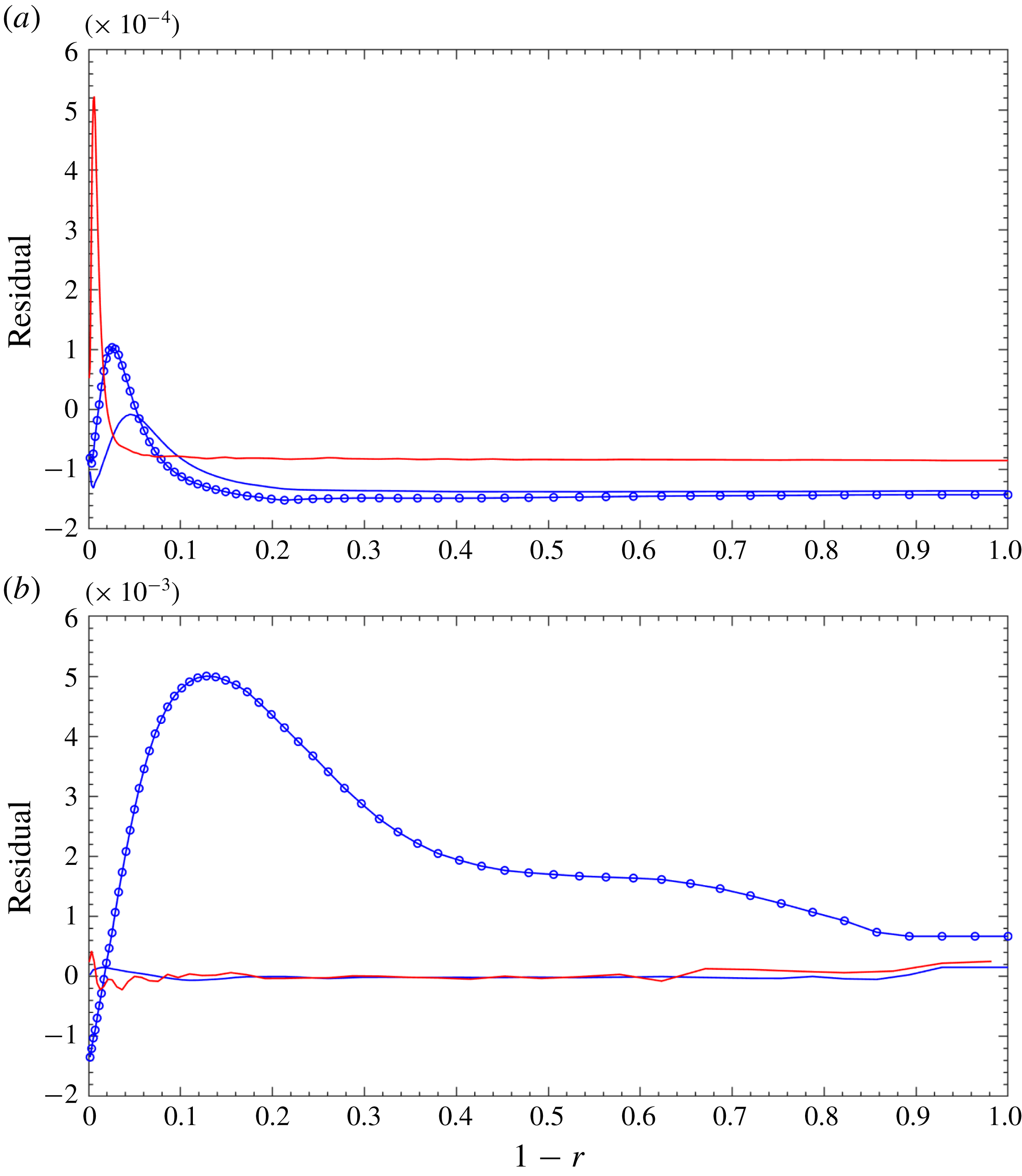
is negligible. The residual of (4.7) is less than
 $5\times 10^{-4}\,(\overline{\mathit{u}}_{\mathit{bulk}}^{2})/R$
, where the larger value is found in the case of the stationary pipe at
 $Re_{D}=44\,000$
, as shown in figure 20(a). For (4.8), the maximum value of the residual is approximately
 $5\times 10^{-3}\,(\overline{\mathit{u}}_{\mathit{bulk}}^{2})/R$
, as shown in figure 20(b). For a stationary pipe,
 $\overline{F}_{r}=0$
, it is not a surprise that the residuals are much smaller. Note that the pattern of the residual profile of the EVM solution at
 $Re_{D}=44\,000$
is quite similar to that presented in Wu & Moin (Reference Wu and Moin2008) in that the larger value is mostly located near the pipe wall.
Residual of the EVM solution of the Reynolds-averaged mean momentum transport equation for pipe flow at
 $Re_{D}=5300$
and
 $Re_{D}=44\,000$
. Blue solid line: stationary pipe at
 $Re_{D}=5300$
; red solid line: stationary pipe at
 $Re_{D}=44\,000$
; blue solid line with circles: vibrating pipe at
 $s_{o}=0.0667,Re_{D}=5300$
. Normalization is with respect to
 $\overline{\mathit{u}}_{\mathit{bulk}}^{2}/R$
. (a) Residual of (4.7); (b) residual of (4.8).

Budget terms of
 $\overline{u}_{z}$
transport equations (4.7) and that of
 $\overline{u}_{r}$
transport equation (4.8) as a function of
 $(1-r)$
. (a) Lines: viscous shear-stress curvature term,
 $((\unicode[STIX]{x1D708}+\unicode[STIX]{x1D708}_{t})/r)(\text{d}\overline{u}_{z}/\text{d}r)$
; lines with triangles: viscous term,
 $(\unicode[STIX]{x1D708}+\unicode[STIX]{x1D708}_{t})(\text{d}^{2}\overline{u}_{z}/\text{d}r^{2})$
; lines with crosses: shear-stress curvature term,
 $-\overline{u_{z}^{\prime }u_{r}^{\prime }}/r$
; lines with circles: gradient of turbulent shear-stress term,
 $-(\text{d}\overline{u_{z}^{\prime }u_{r}^{\prime }})/\text{d}r$
. Blue colour indicates stationary pipe; red colour indicates
 $s_{o}=0.0667$
. (b) Lines:
 $-\unicode[STIX]{x2202}\overline{p}/\unicode[STIX]{x2202}r$
; lines with crosses: anisotropic curvature term,
 $-(\overline{u_{r}^{\prime 2}}-\overline{u_{\unicode[STIX]{x1D703}}^{\prime 2}})/r$
; lines with circles: the radial component of gradient of turbulence fluctuations,
 $-\text{d}\overline{u_{r}^{\prime 2}}/\text{d}r$
. Blue colour indicates stationary pipe; red colour indicates
 $s_{o}=0.0667$
.

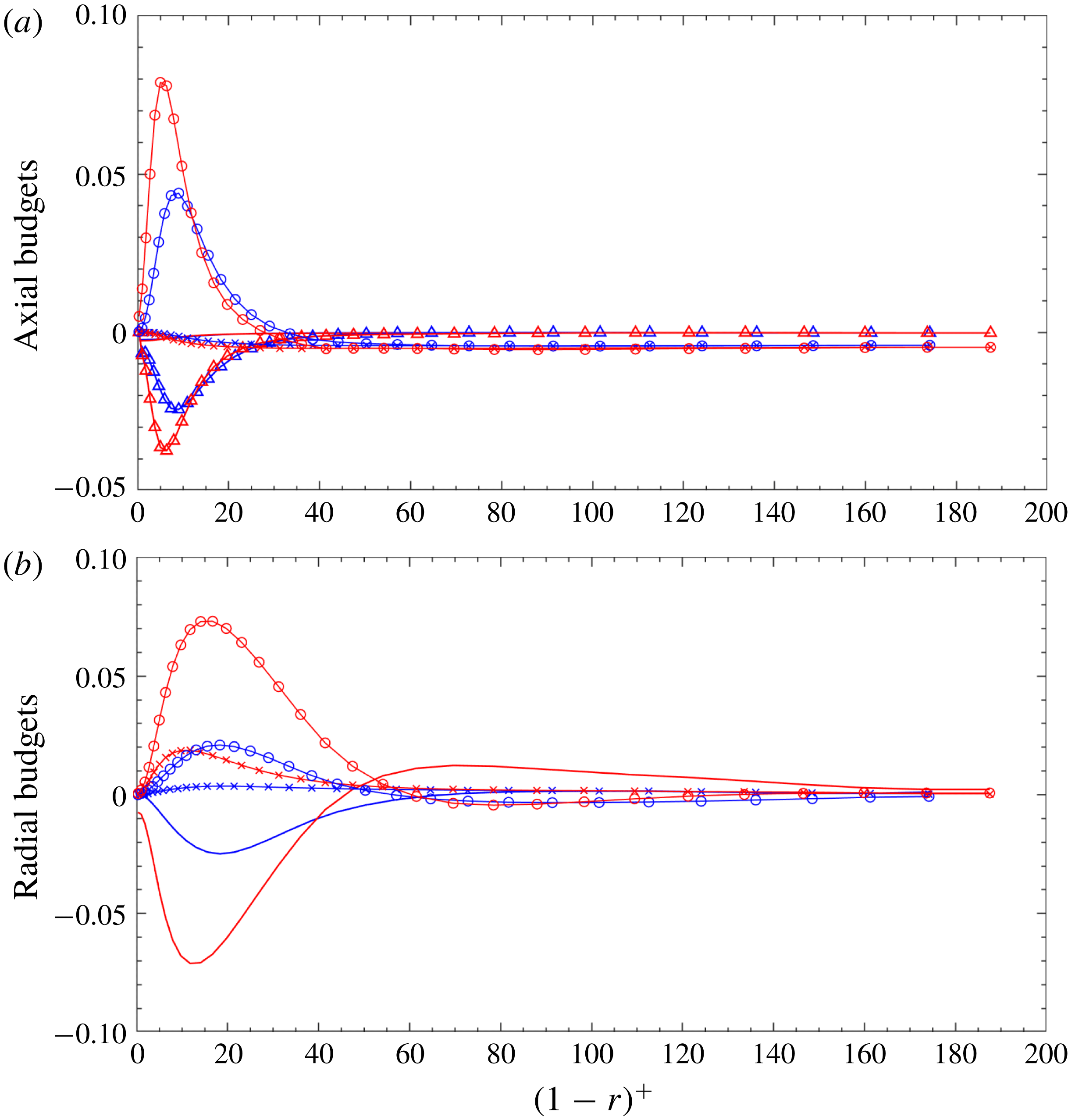
Detailed values of every budget term are useful in theoretical studies of the mean pipe flow velocity profile. In the axial direction,
 $-\unicode[STIX]{x2202}\overline{p}/\unicode[STIX]{x2202}z$
is constant because of the periodicity along the pipe axis. The distribution of the remaining four terms in (4.7) are presented in figure 21(a). The viscous shear-stress curvature term
 $((\unicode[STIX]{x1D708}+\unicode[STIX]{x1D708}_{t})/r)(\text{d}\overline{u}_{z}/\text{d}r)$
(solid lines) has barely changed compared with that of the stationary pipe. In the region of
 $(1-r)^{+}<30$
, the contribution of (4.7) is dominated by the viscous term
 $(\unicode[STIX]{x1D708}+\unicode[STIX]{x1D708}_{t})(\text{d}^{2}\overline{u}_{z}/\text{d}r^{2})$
(lines with triangles) and the gradient of turbulent shear-stress term
 $-\text{d}\overline{u_{z}^{\prime }u_{r}^{\prime }}/\text{d}r$
(lines with circles). In the sub-region of
 $(1-r)^{+}<5$
, the absolute values of the viscous and gradient of turbulent shear-stress terms increase monotonically, while in the other part of sub-region of
 $5<(1-r)^{+}<30$
, the absolute values are decreased. This behaviour is quite similar to that of a stationary pipe, except the inflection point is at
 $(1-r)^{+}=9$
, which is a little bit further away from the pipe wall. The contribution of the shear-stress curvature term
 $-\overline{u_{z}^{\prime }u_{r}^{\prime }}/r$
(lines with crosses) is not important over most of the pipe cross-section and its value is very close to the magnitude of the gradient of turbulent shear-stress term
 $-\text{d}\overline{u_{z}^{\prime }u_{r}^{\prime }}/\text{d}r$
(lines with circles). Additionally, it could be observed that the influence of pipe motion on the shear-stress curvature is very small.
Figure 21(b) shows the budget terms along the radial direction, as they appear in (4.8). It can be observed that the effect of pipe motion on all of the three terms is important, since all three terms increase by a significant amount in the region of
 $(1-r)^{+}<50$
. Similar to turbulent flow in a stationary pipe, for flow in a vibrating pipe, the contribution of the radial gradient of mean pressure
 $-\unicode[STIX]{x2202}\overline{p}/\unicode[STIX]{x2202}r$
is balanced by the combination of the anisotropic curvature term
 $-(\overline{u_{r}^{\prime 2}}-\overline{u_{\unicode[STIX]{x1D703}}^{\prime 2}})/r$
and the gradient of the turbulence fluctuations along the radial direction
 $-\text{d}\overline{u_{r}^{\prime 2}}/\text{d}r$
.
4.3 Visualizations
In the previous subsection, we found that both the mean velocity profiles and turbulence intensities changed substantially due to the pipe motion; in particular, the mean velocity and fluctuations are quite different at a node from those at an anti-node. Here, we present a set of images extracted from the present EVM simulations. These images were created in a straightforward manner by plotting the instantaneous values, without other elaborate post-processing procedures. Note that for the vibrating pipe, the snapshots shown in figures 22(b), 23(b) and 24 are when the
 $x$
component of displacement at anti-nodes reaches its maximum and the
 $y$
component of the displacement is zero.
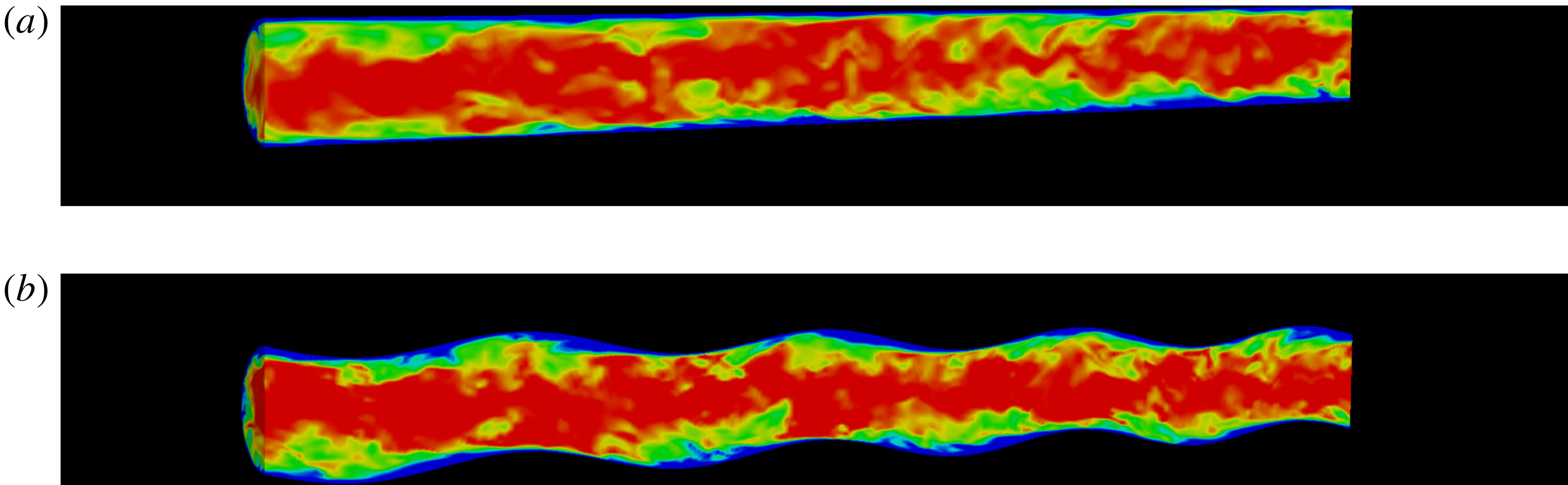
Figure 22 compares the streamwise velocity
 $u_{z}$
of the stationary pipe with that of the vibrating pipe at
 $s_{o}=0.0667$
. Note that in order to see the details inside the pipe, the flow domain shown here is cut at the midplane of the pipe along the axis. In these two images, the magnitude of
 $u_{z}$
is in a range 0.6 (blue) to 1.3 (red). For the stationary pipe, it can be observed that the blue colour low-momentum fluid layer is quite uniform, and some wavy structures are elongated away from the wall towards the downstream direction. However, when the pipe is vibrating, the low-velocity regions depend on the pipe motion: the low-momentum flow is accumulated near the wall behind a crest (anti-node), and its thickness decreases before reaching the next crest.
Visualization of pipe flows using contours of instantaneous streamwise velocity
 $u_{z}$
. (a) Stationary pipe; (b) vibrating pipe at
 $s_{o}=0.0667$
. Red colour indicates high velocity while blue colour indicates low velocity. Flow is from left to right.

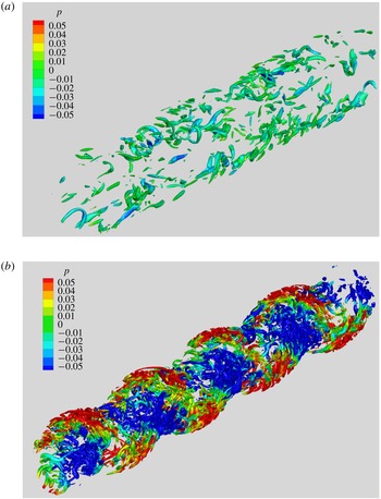
Figure 23 compares the vortices in a vibrating pipe with those in a stationary pipe. In these two images, the vortices are visualized by using the iso-surface of the a positive value of the second invariant of the strain rate tensor, namely
 $Q=20$
. It is quite obvious that when the pipe is vibrating, more worm-like vortices are generated; as discussed in Xie et al. (Reference Xie, Zheng, Triantafyllou, Constantinides and Karniadakis2016), continuous generation of new vorticity due to wall acceleration is shed in the confined space of the interior of the pipe. Furthermore, these vortices are not distributed uniformly over the vibrating pipe, but they are transported and deposited in the troughs where the axial velocity is lower. In figure 23(b), we can also observe that, for flow in a vibrating pipe, the pressure field changes significantly at an anti-node, which reveals the larger pressure fluctuation
 $p_{\mathit{rms}}^{\prime +}$
that is also obtained by our phase-averaged statistics in § 4.1.
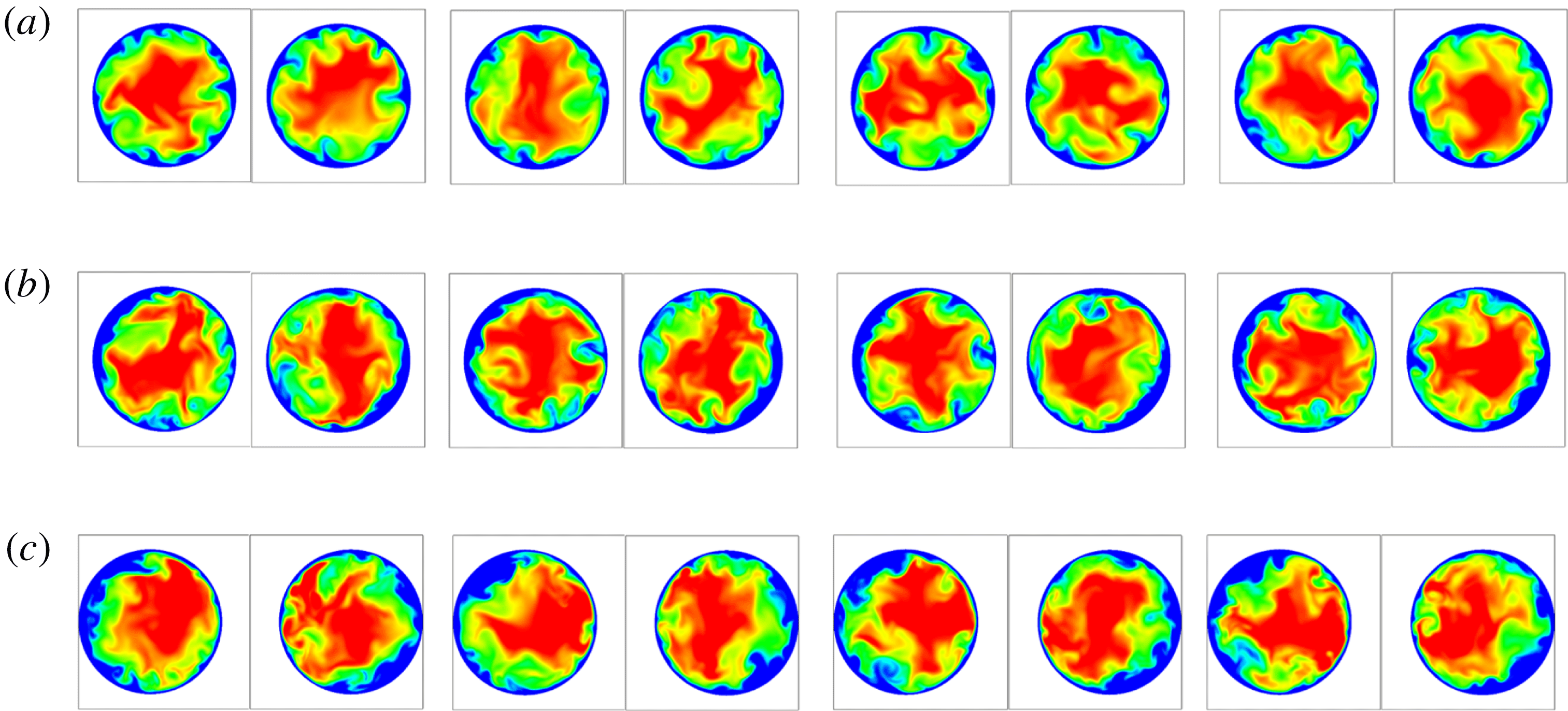
Figure 24(a–c) exhibits the contours at eight cross-sectional planes of the instantaneous streamwise velocity
 $u_{z}$
for the stationary pipe, and the vibrating pipe at the nodes and the anti-nodes, respectively. Note that in these snapshots, the time, the magnitude range of
 $u_{z}$
and the meaning of the colour is the same as that of figure 22. As expected, for the stationary pipe, in the near-wall region, the thickness of the blue colour low-momentum structures is relatively uniform along the azimuthal direction and among different cross-sections. However, for the vibrating pipe, both at nodes and anti-nodes, in the direction that the cross-section is moving (cross-flow plane), the thickness of the low-velocity structures is larger than that in the opposite direction, while the effect of pipe motion on the distribution of the low-velocity structures is more prominent at the anti-nodes than that at the nodes.
Visualization of vortices in pipe flows using instantaneous iso-surface of
 $Q=20$
that is coloured by pressure
 $p$
. (a) Stationary pipe; (b) vibrating pipe at
 $s_{o}=0.0667$
. Flow is from left to right.

Visualization of turbulent pipe flow at eight cross-sectional planes of instantaneous streamwise velocity
 $u_{z}$
. (a) Stationary pipe – the locations of the cross-sections are same as those of (b); (b) cross-sections at the nodes of the vibrating pipe; (c) cross-sections at the anti-nodes of the vibrating pipe. For each image, the square frame around the circular cross-section is
 $[-0.6D,0.6D]\times [-0.6D,0.6D]$
.

4.4 Two-point correlations
In § 4.1 we have shown that the pipe motion enhances greatly the pressure fluctuations, and from the visualization images in § 4.3 we also discovered that the turbulent coherent structures are transported and arranged in patterns that are characterized by negative pressure and positive pressure along the pipe axis, which implies that the turbulent structures are more correlated due to the pipe motion. In this section, we study quantitatively these correlations both spatially and temporarily.
Defining the streamwise separation
 $\unicode[STIX]{x0394}z=z-z^{\prime }$
and azimuthal separation
 $\unicode[STIX]{x0394}\unicode[STIX]{x1D703}=\unicode[STIX]{x1D703}-\unicode[STIX]{x1D703}^{\prime }$
, the two-point correlations of fluctuations of quantity
 $\unicode[STIX]{x1D719}$
as a function of
 $\unicode[STIX]{x0394}z$
and
 $\unicode[STIX]{x0394}\unicode[STIX]{x1D703}$
at a radial location
 $r$
are calculated as follows,
 $$\begin{eqnarray}R_{\unicode[STIX]{x1D719}\unicode[STIX]{x1D719}}(r;\unicode[STIX]{x0394}\unicode[STIX]{x1D703},\unicode[STIX]{x0394}z)={\displaystyle \frac{\langle \unicode[STIX]{x1D719}(r;\unicode[STIX]{x1D703}^{\prime },z^{\prime })\cdot \unicode[STIX]{x1D719}(r;\unicode[STIX]{x1D703}^{\prime }+\unicode[STIX]{x0394}\unicode[STIX]{x1D703},z^{\prime }+\unicode[STIX]{x0394}z)\rangle }{\unicode[STIX]{x1D719}_{\mathit{rms}}(r;\unicode[STIX]{x1D703}^{\prime },z^{\prime })\cdot \unicode[STIX]{x1D719}_{\mathit{rms}}(r;\unicode[STIX]{x1D703}^{\prime }+\unicode[STIX]{x0394}\unicode[STIX]{x1D703},z^{\prime }+\unicode[STIX]{x0394}z)}},\end{eqnarray}$$
where the brackets indicate an average over time. In this section, we consider two radial distances
 $(1-r)=0.01$
and
 $(1-r)=0.5$
, where the former is inside the viscous sublayer (
 $(1-r)^{+}<5$
), while the latter is in the outer layer (
 $(1-r)^{+}>50$
). To obtain the correlations, we have computed the following three cases: stationary pipe,
 $s_{o}=0.0067$
and
 $s_{o}=0.0667$
. For each case, 3500 consecutive snapshots are collected with a time interval of
 $\unicode[STIX]{x0394}t=0.036D/\overline{\mathit{u}}_{\mathit{bulk}}$
. Each of the snapshots has
 $64\times 128$
data points that are uniformly placed along the azimuthal and streamwise directions.
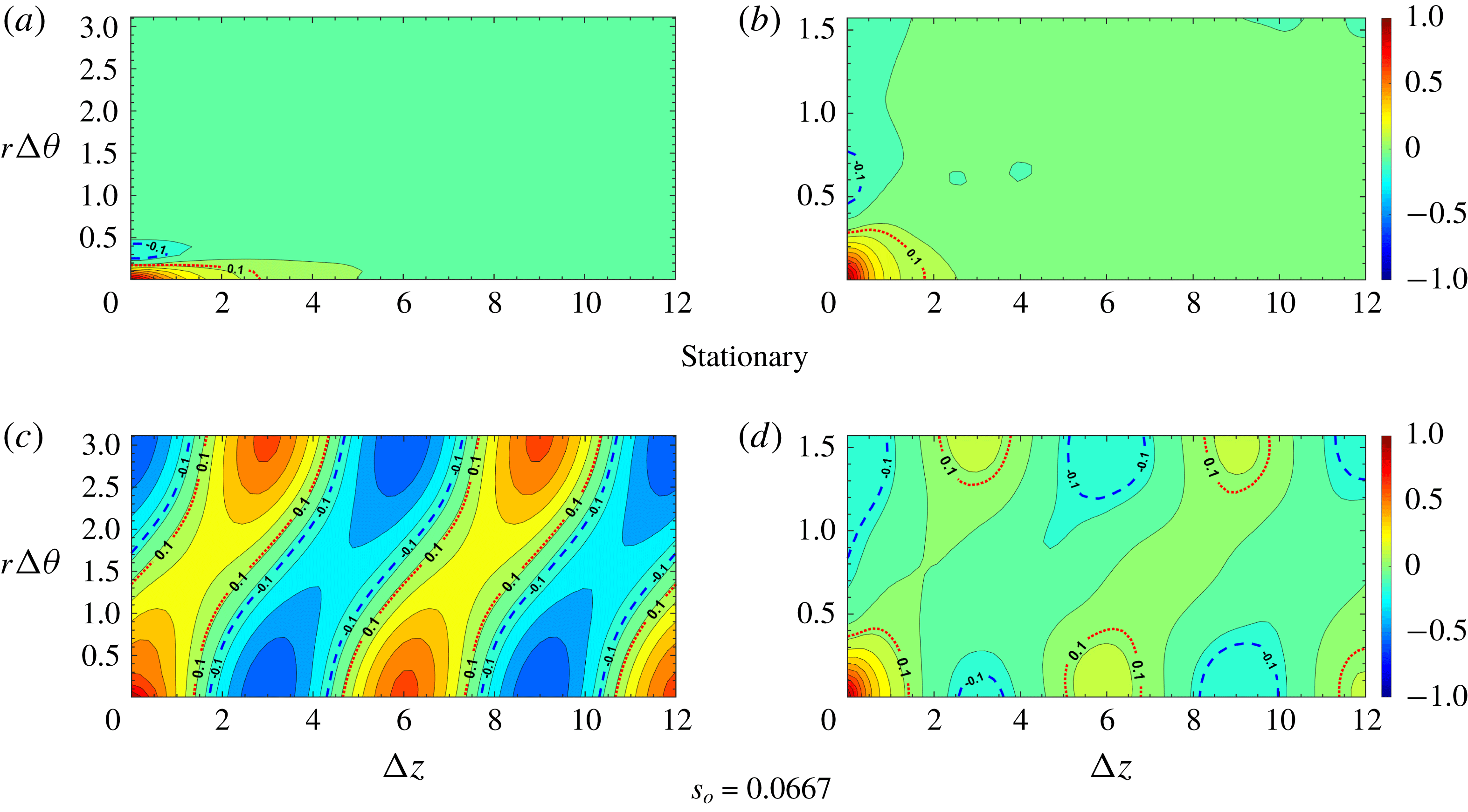
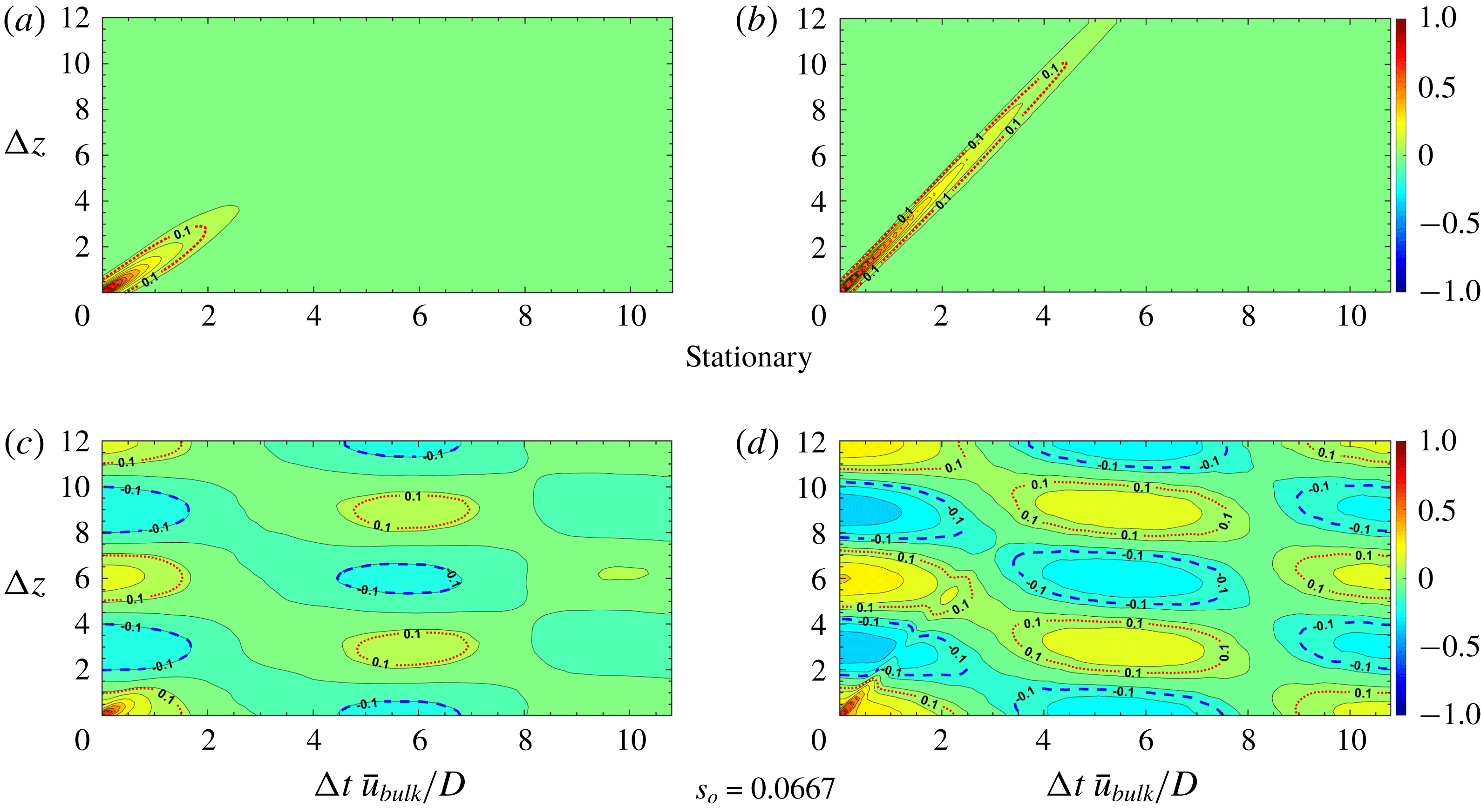
Contours of two-point correlation coefficient
 $R_{u_{z}^{\prime }u_{z}^{\prime }}(\unicode[STIX]{x0394}\unicode[STIX]{x1D703},\unicode[STIX]{x0394}z)$
. Red dashed line, contour level 0.1; blue dashed line, contour level
 $-0.1$
. (a,c) Near wall,
 $1-r=0.01$
; (b,d) away from wall,
 $1-r=0.5$
.

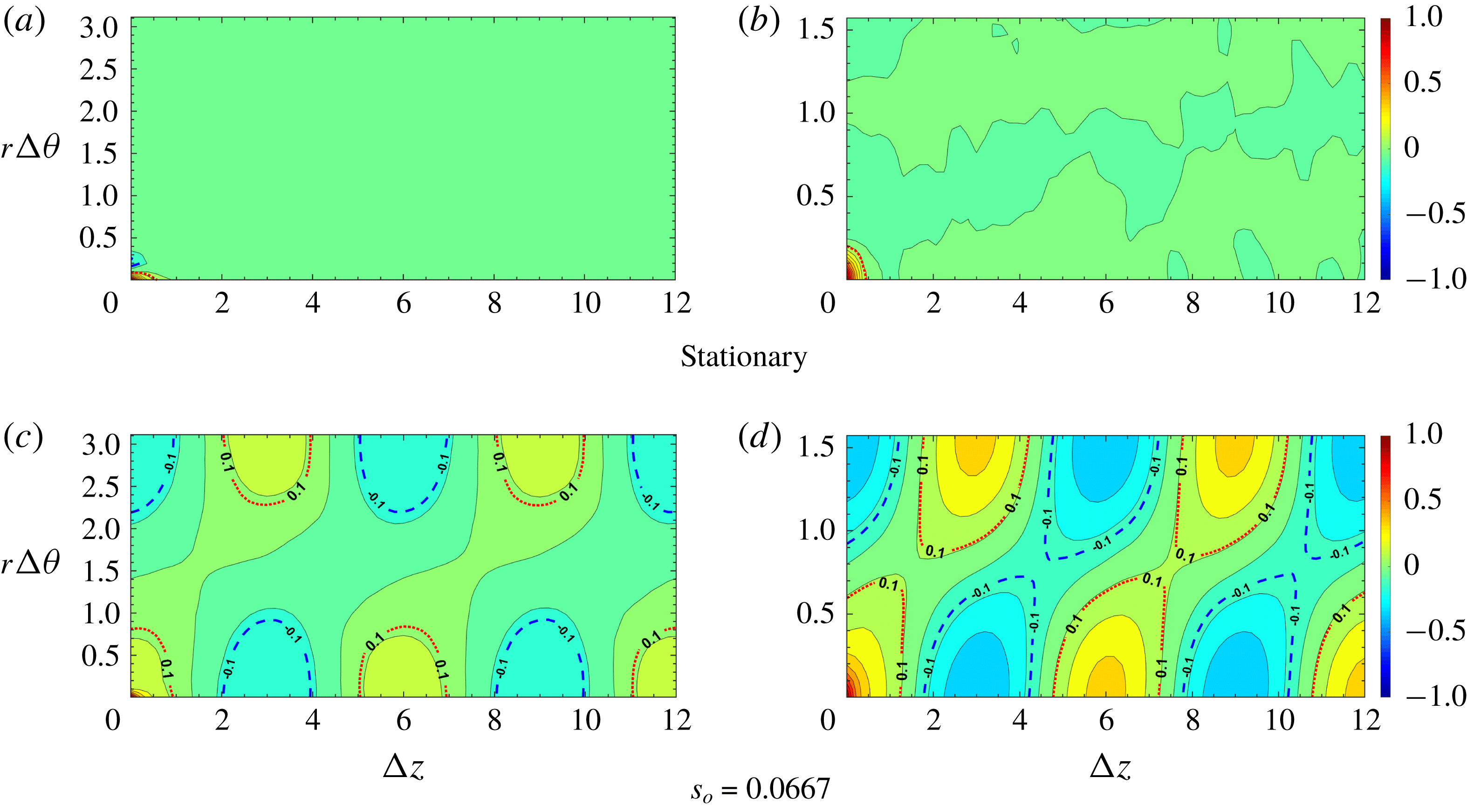
Contours of two-point correlation coefficient
 $R_{u_{r}^{\prime }u_{r}^{\prime }}(\unicode[STIX]{x0394}\unicode[STIX]{x1D703},\unicode[STIX]{x0394}z)$
. Red dashed line, contour level 0.1; blue dashed line, contour level
 $-0.1$
. (a,c) Near wall,
 $1-r=0.01$
; (b,d) away from wall,
 $1-r=0.5$
.

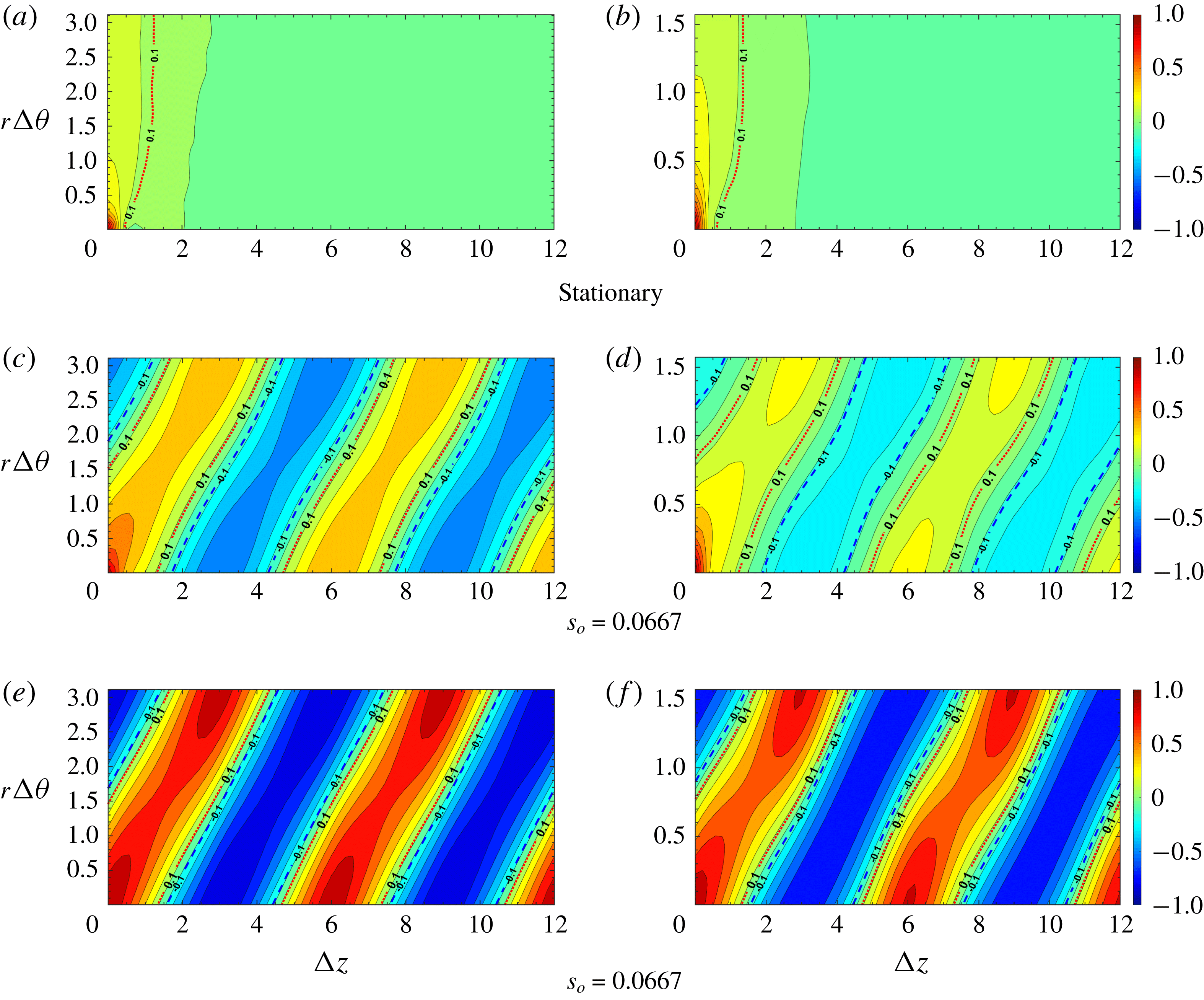
Contours of two-point correlation coefficient
 $R_{p^{\prime }p^{\prime }}(\unicode[STIX]{x0394}\unicode[STIX]{x1D703},\unicode[STIX]{x0394}z)$
. Red dashed line, contour level 0.1; blue dashed line, contour level
 $-0.1$
. (a,c,e) Near wall,
 $1-r=0.01$
; (b,d,f) away from wall,
 $1-r=0.5$
.

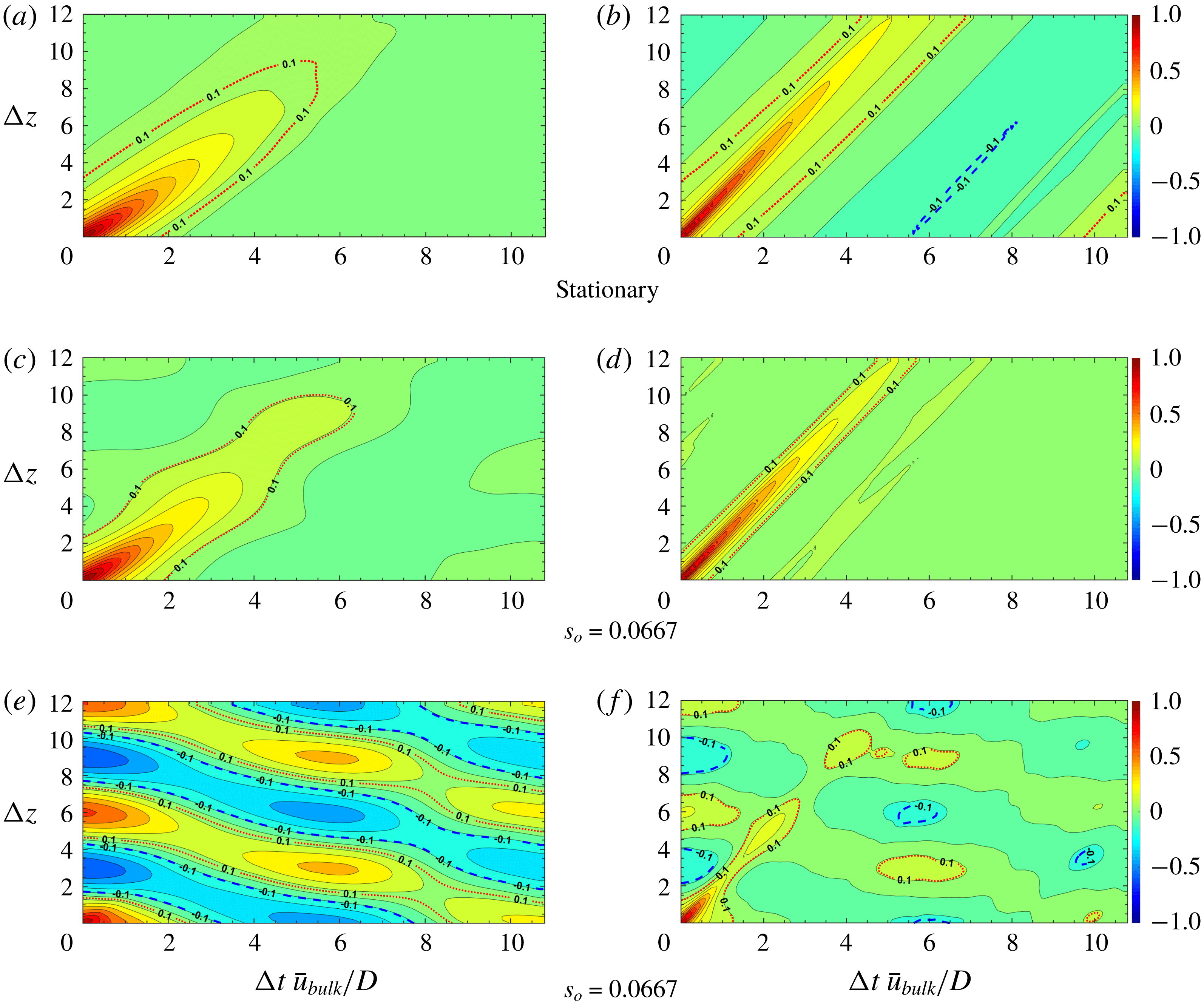
Contours of two-point correlation coefficient
 $R_{u_{z}^{\prime }u_{z}^{\prime }}(\unicode[STIX]{x0394}t,\unicode[STIX]{x0394}z)$
. Red dashed line, contour level 0.1; blue dashed line, contour level
 $-0.1$
. (a,c,e) Near wall,
 $1-r=0.01$
; (b,d,f) away from wall,
 $1-r=0.5$
.

Contours of two-point correlation coefficient
 $R_{u_{r}^{\prime }u_{r}^{\prime }}(\unicode[STIX]{x0394}t,\unicode[STIX]{x0394}z)$
. Red dashed line, contour level 0.1; blue dashed line, contour level
 $-0.1$
. (a,c) Near wall,
 $1-r=0.01$
; (b,d) away from wall,
 $1-r=0.5$
.

The contours of the two-point correlation coefficients
 $R_{u_{z}^{\prime }u_{z}^{\prime }}(r;\unicode[STIX]{x0394}\unicode[STIX]{x1D703},\unicode[STIX]{x0394}z)$
at different
 $1-r$
and
 $s_{o}$
are shown in figure 25. In this figure, the red dashed line represents a contour level of 0.1, while the blue dashed line means a contour level of
 $-0.1$
. For the stationary pipe, the contours of constant
 $R_{u_{z}^{\prime }u_{z}^{\prime }}(r;\unicode[STIX]{x0394}\unicode[STIX]{x1D703},\unicode[STIX]{x0394}z)$
near the pipe wall (
 $1-r=0.01$
) are elongated along the streamwise direction but less so away from the wall (
 $1-r=0.5$
). When the pipe is vibrating at a very small amplitude (
 $s_{o}=0.0067$
), the change of correlation pattern is negligible; as
 $s_{o}$
is increased, the contours of correlation near the wall have a periodic cellular like pattern, while away from the wall and close to the axis the correlation pattern is similar to that of a stationary pipe. Note that the length of the cells bounded by the contour levels
 $0.1$
or
 $-0.1$
is consistent with the prescribed standing-wave motion shown in (4.1), both along the azimuthal and streamwise direction. In figure 26, the contours of
 $R_{u_{r}^{\prime }u_{r}^{\prime }}(r;\unicode[STIX]{x0394}\unicode[STIX]{x1D703},\unicode[STIX]{x0394}z)$
also exhibit a strong periodic cellular pattern at both
 $1-r$
locations, providing that
 $s_{o}\geqslant 0.0333$
. Note that the correlation of the azimuthal component, i.e. the contours of
 $R_{u_{\unicode[STIX]{x1D703}}^{\prime }u_{\unicode[STIX]{x1D703}}^{\prime }}(r;\unicode[STIX]{x0394}\unicode[STIX]{x1D703},\unicode[STIX]{x0394}z)$
are quite similar to those of
 $R_{u_{r}^{\prime }u_{r}^{\prime }}(r;\unicode[STIX]{x0394}\unicode[STIX]{x1D703},\unicode[STIX]{x0394}z)$
, thus we do not include the corresponding plots here. The most pronounced changes on correlation could be observed from the contours of
 $R_{p^{\prime }p^{\prime }}(r;\unicode[STIX]{x0394}\unicode[STIX]{x1D703},\unicode[STIX]{x0394}z)$
, as shown in figure 27. From this figure, we can observe that for the stationary pipe, the contour lines near the wall are generally elongated along the azimuthal direction and they are more elongated away from the wall, which is different from the plane channel flow results presented in Kim (Reference Kim1989). Nonetheless, the contours of
 $R_{p^{\prime }p^{\prime }}(r;\unicode[STIX]{x0394}\unicode[STIX]{x1D703},\unicode[STIX]{x0394}z)$
change to oblique band type, even for the case that
 $s_{o}$
is as small as 0.0067, at which the change of correlation of the velocity fluctuations is negligible. The dramatic changes in
 $R_{p^{\prime }p^{\prime }}(r;\unicode[STIX]{x0394}\unicode[STIX]{x1D703},\unicode[STIX]{x0394}z)$
reveal the fact that the pressure fluctuations are influenced globally by the pipe motion, as shown in the (4.6).
Next, following the work of Kim & Sung (Reference Kim and Sung2006), we define the space–time correlation as follows,
 $$\begin{eqnarray}R_{\unicode[STIX]{x1D719}\unicode[STIX]{x1D719}}(r;\unicode[STIX]{x0394}z,\unicode[STIX]{x0394}t)={\displaystyle \frac{\langle \unicode[STIX]{x1D719}(r;z^{\prime },t^{\prime })\cdot \unicode[STIX]{x1D719}(r;z^{\prime }+\unicode[STIX]{x0394}z,t^{\prime }+\unicode[STIX]{x0394}t)\rangle }{\unicode[STIX]{x1D719}_{\mathit{rms}}(r;z^{\prime },t^{\prime })\cdot \unicode[STIX]{x1D719}_{\mathit{rms}}(r;z^{\prime }+\unicode[STIX]{x0394}z,t^{\prime }+\unicode[STIX]{x0394}t)}},\end{eqnarray}$$
where the brackets in (4.10) mean an averaging over the streamwise and azimuthal directions, respectively. The space–time correlations with respect to
 $\unicode[STIX]{x0394}z$
and
 $\unicode[STIX]{x0394}t$
are presented in figures 28–30. In the stationary pipe or vibrating pipe at small
 $s_{o}$
, as shown in figure 28, we observe that the contours of
 $R_{u_{z}^{\prime }u_{z}^{\prime }}(r;\unicode[STIX]{x0394}z,\unicode[STIX]{x0394}t)$
show a prominent band-type pattern that stretches from bottom left to top right. However, as
 $s_{o}$
increases, the contours of
 $R_{u_{z}^{\prime }u_{z}^{\prime }}(r;\unicode[STIX]{x0394}z,\unicode[STIX]{x0394}t)$
at
 $1-r=0.01$
exhibit a periodic cellular structure close to the wall, while at
 $1-r=0.5$
, the correlation structure remains the same as in the stationary case. In contrast, the correlation contours of
 $R_{u_{r}^{\prime }u_{r}^{\prime }}(r;\unicode[STIX]{x0394}z,\unicode[STIX]{x0394}t)$
and
 $R_{u_{\unicode[STIX]{x1D703}}^{\prime }u_{\unicode[STIX]{x1D703}}^{\prime }}(r;\unicode[STIX]{x0394}z,\unicode[STIX]{x0394}t)$
(not included in this paper) exhibit a cellular structure both at the wall and close to the pipe axis. Finally, as before, the pressure correlation in terms of
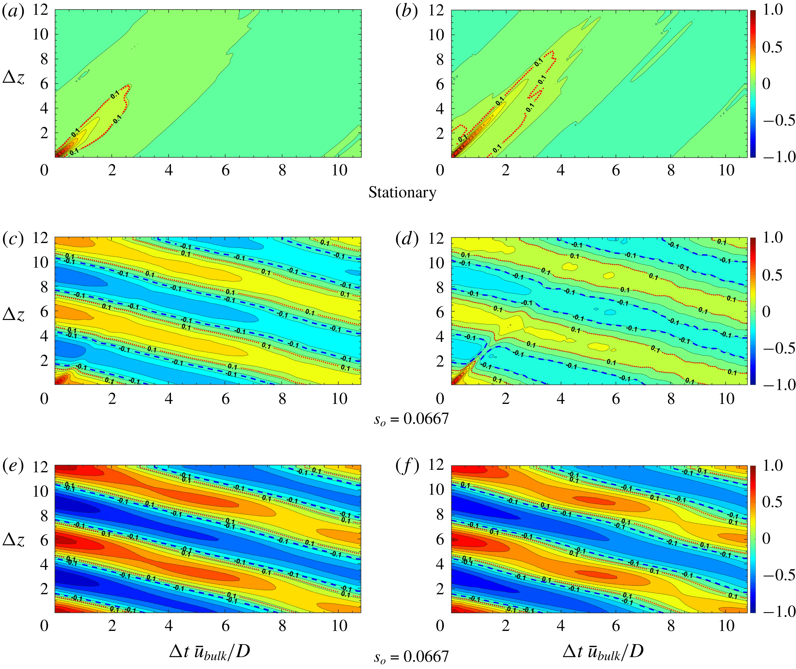
 $R_{p^{\prime }p^{\prime }}(r;\unicode[STIX]{x0394}z,\unicode[STIX]{x0394}t)$
is more sensitive to pipe motions, as shown in figure 30. We observe that, at small
 $s_{o}=0.0067$
, the pattern of the correlation contours changes from a positive slope band to a negative slope band at both
 $1-r$
locations, although at
 $1-r=0.0067$
, a small band with positive slope still exists in the bottom left of figure 30(b). The positive slope band disappears as
 $s_{o}$
is increased.
Contours of two-point correlation coefficient
 $R_{p^{\prime }p^{\prime }}(\unicode[STIX]{x0394}t,\unicode[STIX]{x0394}z)$
. Red dashed line, contour level 0.1; blue dashed line, contour level
 $-0.1$
. (a,c,e) Near wall,
 $1-r=0.01$
; (b,d,f) away from wall,
 $1-r=0.5$
.

5 Summary
There are two contributions in the present paper, the first on the LES methodology and the second on quantifying the statistics of fully developed incompressible turbulent flow in a flexible pipe. In particular, the entropy-viscosity method (EVM) presented herein may be viewed as an alternative LES approach, similar to implicit-type LES but with an additional viscous stabilization term (that of the entropy viscosity) to dissipate the energy due to unresolved small scales. This method was first introduced by Guermond (Reference Guermond2008) for preserving monotonicity in aerodynamic flows but just like other dissipative mechanisms, e.g. the spectral vanishing viscosity, it can also be used in under-resolved simulations of turbulent flow. We introduced a new formula for calculating the entropy viscosity without free parameters by drawing an analogy with the standard Smagorinsky model – an intuitive argument that was tested against direct numerical simulations of homogeneous isotropic turbulence as well as fully developed turbulent pipe flow (Wu & Moin Reference Wu and Moin2008). It is rather difficult to quantify a priori at what reduced resolution EVM-based simulations can be accurate, but in the present work we have employed grids with a resolution approximately two orders of magnitude lower than the DNS. We also need to clarify that this comparison should take into account the discretization method; for example, here we employed spectral element discretization in Cartesian coordinates whereas in Wu & Moin (Reference Wu and Moin2008) they employed second-order finite difference discretization in cylindrical coordinates. A more thorough validation study for different complex-geometry flows will be presented in future publication. A key advantage of EVM is that it does not depend on the mesh type or polynomial interpolation. The novelty is that a nonlinear viscosity based on the local size of an entropy production is added to the selected numerical discretization. EVM does not use any flux or slope limiters unlike other methods in implicit LES.
In the second part of the paper, we simulated fully developed turbulent flow at
 $Re_{D}=5300$
in a flexible pipe subject to prescribed vibrations in the cross-flow plane corresponding to a standing wave. We simulated 11 cases corresponding to increasing values of wave steepness
 $s_{o}$
, and we found a quadratic dependence of the friction factor on
 $s_{o}$
with a small drag reduction at small amplitude excitation. In terms of second-order statistics, we found substantial changes in the peaks of turbulent intensities, which were amplified by
 $50\,\%$
in the axial direction and by
 $200\,\%$
in the normal and azimuthal directions at
 $s_{o}=0.067$
. Correspondingly, the peak shear stress at the node increased by more than
 $300\,\%$
whereas at the anti-node it exhibited (small) negative values. Specifically, the statistics at the nodes and anti-nodes have very different trends and magnitudes. For example, the streamwise turbulent intensity at a node is greater than that at an anti-node in the region of
 $0<(1-r)^{+}<15$
, but smaller farther from the wall. In contrast, the azimuthal turbulent intensity is the same for the node and anti-node in the range
 $0<(1-r)^{+}<25$
but farther away from the wall the turbulent intensity at the node, surprisingly, is much larger. Our current first simulations of a flexible pipe demonstrate that turbulent flow even at relatively low Reynolds number is highly affected by the wall motion and is very different from the fully developed turbulent flow in a stationary pipe.
Effect of parameter
 $\unicode[STIX]{x1D6FC}$
on dimensionless energy spectra
 $E(k)/(\unicode[STIX]{x1D708}^{5}\unicode[STIX]{x1D700})^{1/4}$
as a function of
 $k\,\unicode[STIX]{x1D702}$
. Blue solid circle: experimental energy spectra in Comte-Bellot & Corrsin (Reference Comte-Bellot and Corrsin1971) at
 $Re_{\unicode[STIX]{x1D706}}=60.7$
; black dashed line: no EVM; black dotted line:
 $\unicode[STIX]{x1D6FC}=0.05$
; red solid line with triangle:
 $\unicode[STIX]{x1D6FC}=0.45$
; red solid line:
 $\unicode[STIX]{x1D6FC}=0.5$
; red solid line with square:
 $\unicode[STIX]{x1D6FC}=0.55$
; green line:
 $\unicode[STIX]{x1D6FC}=1.0$
.

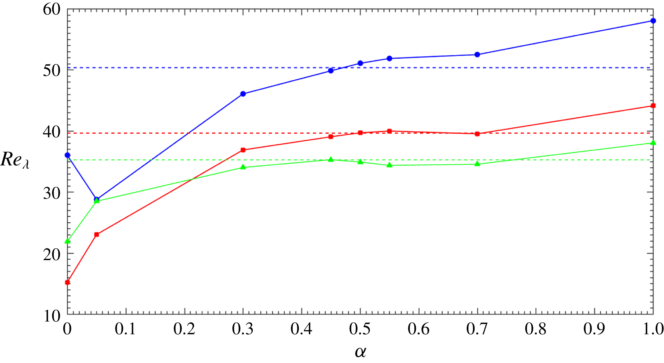
Comparison of EVM results of Taylor-scale Reynolds number
 $Re_{\unicode[STIX]{x1D706}}=(\sqrt{20/3})((\int _{0}^{\infty }E(k)\,\text{d}k)/\unicode[STIX]{x1D708}(\int _{0}^{\infty }k^{2}\,E(k)\text{d}k)^{1/2})$
varying with parameter
 $\unicode[STIX]{x1D6FC}$
, at time
 $t=20$
(blue solid line with circles),
 $40$
(red solid line with squares) and
 $t=60$
(green solid line with triangles). Dashed lines are results of LES using the finite difference code with a dynamic Smagorinsky model, see Orlandi (Reference Orlandi2000).

Sensitivity of mean axial velocity
 $\overline{u_{z}}^{+}$
to parameter
 $\unicode[STIX]{x1D6FC}$
. (a)
 $Re_{D}=5300$
; (b)
 $Re_{D}=44\,000$
.

Acknowledgements
The authors gratefully acknowledge support by the Chevron-MIT University Partnership Program and the ESRDC ONR project. The simulations were performed on the parallel cluster of the Center for Computation & Visualization at Brown University.
Appendix A. Simulation results of decay of homogeneous isotropic turbulence
In this section, EVM is applied to simulating the decay of homogeneous isotropic turbulence (HIT). We have implemented the EVM in a three-dimensional incompressible solver employing the same splitting scheme as in Karniadakis & Sherwin (Reference Karniadakis and Sherwin2005) in the framework of the open source finite element library Deal.II (Arndt et al.
Reference Arndt, Bangerth, Davydov, Heister, Heltai, Kronbichler, Maier, Pelteret, Turcksin and Wells2017). In particular, we studied the sensitivity of the simulation results to the parameter
 $\unicode[STIX]{x1D6FC}$
.
Prescribing initial conditions of HIT for a Navier–Stokes equation in physical space is very complicated. Here, in light of Orlandi (Reference Orlandi2000), a random and isotropic field with a prescribed energy spectrum is generated. The energy spectrum is given by the following formula,
 $$\begin{eqnarray}E(k)={\displaystyle \frac{q^{2}}{2k_{p}A}}\left({\displaystyle \frac{k}{k_{p}}}\right)^{\unicode[STIX]{x1D70E}}\text{exp}\left[-{\displaystyle \frac{\unicode[STIX]{x1D70E}}{2}}\left({\displaystyle \frac{k}{k_{p}}}\right)^{2}\right],\end{eqnarray}$$
where
 $k_{p}=13$
is the wavenumber at which
 $E(k)$
is maximum,
 $\unicode[STIX]{x1D70E}=2$
is a parameter and
 $A=\int _{0}^{\infty }\text{exp}(-\unicode[STIX]{x1D70E}(k^{2}/2))\,\text{d}k$
, where
 $q^{2}=3$
. The kinematic viscosity is
 $\unicode[STIX]{x1D708}=1/3000$
.
The discrete Fourier transform (DFT) is used to convert the velocity field from wavenumber space into physical space. We note that DFT requires an equal size mesh, therefore numerical interpolation was employed in order to convert values on a uniform mesh to the Gauss quadrature points. The computational domain is
 $[-\unicode[STIX]{x03C0},\unicode[STIX]{x03C0}]^{3}$
. For the cases presented in this section, the domain is divided into
 $40^{3}$
elements uniformly, with periodic boundary conditions on all sides. The first-order Lagrange polynomial (
 $Q1/Q1$
element) was employed for both velocity and pressure space and the
 $3/2$
quadrature rule was used. To fully validate our implementation, we also conducted simulations by a finite difference method (FDM) code using a second-order central difference scheme, provided by Orlandi (Reference Orlandi2000). Note that in order to have the same kinetic energy as the EVM simulation, in the FDM simulation, the domain was partitioned into
 $60^{3}$
uniform cubes.
Figure 31 presents the simulation results of energy spectrum
 $E(k)/(\unicode[STIX]{x1D708}^{5}\unicode[STIX]{x1D700})^{1/4}$
as a a function of
 $k\,\unicode[STIX]{x1D702}$
at
 $t=20$
, where
 $\unicode[STIX]{x1D702}=(\unicode[STIX]{x1D708}^{3}/\unicode[STIX]{x1D700})^{1/4}$
is the Kolmogorov scale. It can be observed that the energy spectra of EVM match with the measurements of Comte-Bellot & Corrsin (Reference Comte-Bellot and Corrsin1971) quite well, when
 $\unicode[STIX]{x1D6FC}$
is in a region close to 0.5 (red lines with symbols), e.g. in a region of
 $[-0.45,0.55]$
. When
 $\unicode[STIX]{x1D6FC}=1.0$
(green line), the energy spectrum is underestimated, which implies
 $\unicode[STIX]{x1D6FC}=1.0$
is over-dissipative. When
 $\unicode[STIX]{x1D6FC}=0.05$
or no EVM (black dashed line and dotted line), the energy spectra deviate from the experimental spectrum significantly.
Figure 32 shows the variation of Taylor-scale Reynolds number
 $Re_{\unicode[STIX]{x1D706}}=(\sqrt{20/3})((\int _{0}^{\infty }E(k)\,\text{d}k)/(\unicode[STIX]{x1D708}(\int _{0}^{\infty }k^{2}\,E(k)\,\text{d}k)^{1/2}))$
with
 $\unicode[STIX]{x1D6FC}$
, at
 $t=20$
, 40 and
 $t=60$
. From this figure, we can also conclude that
 $Re_{\unicode[STIX]{x1D706}}$
is not sensitive to
 $\unicode[STIX]{x1D6FC}$
when
 $\unicode[STIX]{x1D6FC}$
is in a range of
 $[0.45,0.55]$
.
Sensitivity of axial turbulence intensity
 $u_{z,rms}^{\prime +}$
to parameter
 $\unicode[STIX]{x1D6FC}$
. (a)
 $Re_{D}=5300$
; (b)
 $Re_{D}=44\,000$
.

Sensitivity of turbulent shear stress
 $\overline{u_{z}^{\prime }u_{r}^{\prime }}^{+}$
to parameter
 $\unicode[STIX]{x1D6FC}$
. (a)
 $Re_{D}=5300$
; (b)
 $Re_{D}=44\,000$
.

Sensitivity of intensity of pressure fluctuations
 $p_{\mathit{rms}}^{\prime +}$
to parameter
 $\unicode[STIX]{x1D6FC}$
. (a)
 $Re_{D}=5300$
; (b)
 $Re_{D}=44\,000$
.

Sensitivity of normalized entropy viscosity to parameter
 $\unicode[STIX]{x1D6FC}$
. Note the black-dotted line is the
 $O(1-r)^{3}$
scaling law. (a)
 $Re_{D}=5300$
; (b)
 $Re_{D}=44\,000$
.

Stationary pipe flow at
 $Re=5300$
(a–d) and
 $Re_{D}=44\,000$
(e–h): over the middle cross-section, comparison of the entropy viscosity (
 $\unicode[STIX]{x1D708}_{\mathit{E}}$
) and the numerical viscosity of first-order upwind scheme (
 $\unicode[STIX]{x1D708}_{\mathit{max}}$
) by varying
 $\unicode[STIX]{x1D6FC}$
. Red area represents
 $\unicode[STIX]{x1D708}_{\mathit{E}}\geqslant \unicode[STIX]{x1D708}_{\mathit{max}}$
, blue area represents
 $\unicode[STIX]{x1D708}_{\mathit{E}}<\unicode[STIX]{x1D708}_{\mathit{max}}$
.

Mean axial velocity
 $\overline{u_{z}}^{+}$
as a function
 $(1-r)$
, at
 $Re_{D}=5300$
. Black solid line: Wu & Moin (Reference Wu and Moin2008); magenta pentagrams: EVM with
 $M=2$
; blue triangles: EVM with
 $M=3$
; red squares: EVM with
 $M=4$
; green circles: EVM with
 $M=5$
; cyan hexagrams: EVM with
 $M=6$
.

Axial turbulence intensity
 $u_{z,rms}^{\prime +}$
as a function of
 $(1-r)$
. For details see figure 39.

Turbulent shear stress
 $\overline{u_{z}^{\prime }u_{r}^{\prime }}^{+}$
as a function of
 $(1-r)$
. For details see figure 39.

Mean axial velocity
 $\overline{u_{z}}^{+}$
as a function of
 $(1-r)$
, at
 $Re_{D}=44\,000$
. Black solid line: Wu & Moin (Reference Wu and Moin2008); blue triangles: EVM with
 $M=5$
; red squares: EVM with
 $M=7$
; green circles: EVM with
 $M=8$
.

Axial turbulence intensity
 $u_{z,rms}^{\prime +}$
as a function of
 $(1-r)$
. For details see figure 42.

Turbulent shear stress
 $\overline{u_{z}^{\prime }u_{r}^{\prime }}^{+}$
as a function of
 $(1-r)$
. For details see figure 42.

Appendix B. Sensitivity to parameters
$\unicode[STIX]{x1D6FC}$
and
$\unicode[STIX]{x1D6FD}$


In appendix A we have shown that the EVM solution is not very sensitive to
 $\unicode[STIX]{x1D6FC}$
in a range centred around 0.5 for HIT. In this section, we will study the sensitivity of EVM solution to parameter
 $\unicode[STIX]{x1D6FC}$
by systematically tuning it in a range
 $[0.0005,0.05]$
for pipe flow at
 $Re_{D}=5300$
and
 $[0.0025,0.05]$
for pipe flow at
 $Re_{D}=44\,000$
. In order to investigate the effect of
 $\unicode[STIX]{x1D6FC}$
, we have performed simulations at a lower resolution, specifically, we have employed second-order Jacobi polynomials,
 $64$
Fourier planes and
 $\unicode[STIX]{x0394}t=3\times 10^{-3}$
for the flow at
 $Re_{D}=5300$
, and fifth-order Jacobi polynomials,
 $256$
Fourier planes and
 $\unicode[STIX]{x0394}t=4\times 10^{-4}$
for the flow at
 $Re_{D}=44\,000$
. The statistical sampling duration is
 $500D/\overline{\mathit{u}}_{bulk}$
and
 $100D/\overline{\mathit{u}}_{bulk}$
for the simulation at
 $Re_{D}=5300$
and
 $Re_{D}=44\,000$
, respectively. It is worth noting that, at the above resolution, the EVM simulations with
 $\unicode[STIX]{x1D6FC}<0.0005$
at
 $Re_{D}=5300$
and
 $\unicode[STIX]{x1D6FC}<0.0025$
at
 $Re_{D}=44\,000$
were not stable.
Figure 33 exhibits the mean axial velocity
 $\overline{u_{z}}^{+}$
at various
 $\unicode[STIX]{x1D6FC}$
. For the cases that
 $\unicode[STIX]{x1D6FC}$
is in the range
 $[0.0005,0.01]$
, EVM produces accurate mean axial velocity profile at both Reynolds numbers. At
 $Re_{D}=5300$
, for the cases that
 $\unicode[STIX]{x1D6FC}\geqslant 0.05$
, and at
 $Re_{D}=44\,000$
, for the cases that
 $\unicode[STIX]{x1D6FC}=0.1$
, notable discrepancy from DNS is observed. Figure 34 plots the sensitivity of the axial turbulence intensity
 $u_{z,rms}^{\prime +}$
to
 $\unicode[STIX]{x1D6FC}$
. Again, we could observe that EVM gives rise to good results for
 $\unicode[STIX]{x1D6FC}$
in the range
 $[0.0005,0.01]$
at both Reynolds numbers and it underpredicts
 $u_{z,rms}^{\prime +}$
when
 $\unicode[STIX]{x1D6FC}\geqslant 0.05$
at small Reynolds number and
 $\unicode[STIX]{x1D6FC}=0.1$
at high Reynolds number. The sensitivity of turbulent shear stress
 $\overline{u_{z}^{\prime }u_{r}^{\prime }}^{+}$
to
 $\unicode[STIX]{x1D6FC}$
can be found in figure 35. Apparently, at
 $Re_{D}=5300$
, the prediction matches with DNS very well when
 $\unicode[STIX]{x1D6FC}$
is in the range
 $[0.0005,0.01]$
. At
 $Re_{D}=44\,000$
, the EVM solution begins to deviate from that of DNS when
 $\unicode[STIX]{x1D6FC}\geqslant 0.025$
in the radial position close to the pipe axis. The intensity of pressure fluctuations
 $p_{\mathit{rms}}^{\prime +}$
seem to be more correlated with
 $\unicode[STIX]{x1D6FC}$
. As shown in figure 36, a relatively larger deviation is found near the wall and axis. The near-wall deviation could be reduced by improving the resolution, see figure 7. Because of the low resolution, there is some oscillation of
 $p_{\mathit{rms}}^{\prime +}$
near the pipe axis. The oscillation could be suppressed by increasing the value of
 $\unicode[STIX]{x1D6FC}$
. The averaged normalized entropy viscosity is plotted in figure 37. It could be observed that the magnitude of entropy viscosity increases with
 $\unicode[STIX]{x1D6FC}$
monotonically at both Reynolds numbers. More importantly, the value of entropy viscosity exhibits the correct scaling of
 $O(1-r)^{3}$
in the buffer layer (
 $5<(1-r)^{+}<30$
) when
 $\unicode[STIX]{x1D6FC}<0.01$
.
Overall, we have observed that the EVM results are not sensitive to specific values of
 $\unicode[STIX]{x1D6FC}$
provided that we are in the proper range. We would recommend
 $\unicode[STIX]{x1D6FC}\approx 0.005$
for simulation of pipe flow, and it is safe to use it if
 $\unicode[STIX]{x1D6FC}$
is in the range
 $[0.0025,0.01]$
: below the lower bound, EVM could overpredict the pressure fluctuations near the pipe axis, where the mesh size is coarse; beyond the upper bound, it is likely that EVM will underpredict the velocity fluctuations.
With the value of
 $\unicode[STIX]{x1D6FC}$
in the range
 $[0.0025,0.01]$
, typically, in each element, the entropy viscosity
 $\unicode[STIX]{x1D708}_{\mathit{E}}=\unicode[STIX]{x1D736}(\Vert R_{ijm}^{K}(\mathit{u})\Vert _{L^{\infty }(K)}/\Vert E_{ijm}^{K}(\mathit{u})-\bar{E}(\mathit{u})\Vert _{L^{\infty }(\unicode[STIX]{x1D6FA})})\unicode[STIX]{x1D6FF}_{K}^{2}$
(second term in (2.3)), is at least two orders smaller than the corresponding
 $\unicode[STIX]{x1D708}_{\mathit{max}}=\boldsymbol{\unicode[STIX]{x1D6FD}}\Vert \mathit{u}\Vert _{L^{\infty }(K)}\unicode[STIX]{x1D6FF}_{K}$
, therefore the upper bound in (2.3) was never activated in the current simulations. Nonetheless, for pipe flow, we have performed more simulations by further increasing the value of
 $\unicode[STIX]{x1D6FC}$
close to that of
 $\unicode[STIX]{x1D6FD}$
, so we could observe that
 $\unicode[STIX]{x1D708}_{\mathit{E}}$
exceeds
 $\unicode[STIX]{x1D708}_{\mathit{max}}$
in the area near the axis. Figure 38 shows the comparison of
 $\unicode[STIX]{x1D708}_{\mathit{E}}$
and
 $\unicode[STIX]{x1D708}_{\mathit{max}}$
at the middle plane for both
 $Re_{D}=5300$
and
 $Re_{D}=44\,000$
. In these plots, the red area means
 $\unicode[STIX]{x1D708}_{\mathit{E}}\geqslant \unicode[STIX]{x1D708}_{\mathit{max}}$
, while the blue colour means
 $\unicode[STIX]{x1D708}_{\mathit{E}}<\unicode[STIX]{x1D708}_{\mathit{max}}$
. As expected, when
 $\unicode[STIX]{x1D6FC}\leqslant 0.1$
,
 $\unicode[STIX]{x1D708}_{\mathit{E}}$
never exceeds
 $\unicode[STIX]{x1D708}_{\mathit{max}}$
at both Reynolds numbers, but further increasing
 $\unicode[STIX]{x1D6FC}$
, we observe that the red area for which
 $\unicode[STIX]{x1D708}_{\mathit{E}}\geqslant \unicode[STIX]{x1D708}_{\mathit{max}}$
first appears near the pipe axis and then it expands towards the wall.
Appendix C. Resolution studies of stationary pipe at
$Re_{D}=5300$
and
$Re_{D}=44\,000$


Resolution studies were performed by varying the Jacobi polynomial order
 $M$
on a mesh consisting of 576 quadrilateral elements;
 $\unicode[STIX]{x1D6FC}=0.005$
was used for all computations. At
 $Re_{D}=5300$
, we have employed resolutions consisting of
 $M=2,3,4,5$
with 128 Fourier planes and a highest resolution consisting of
 $M=6$
with 512 Fourier planes that is close to the resolution of the DNS in Wu & Moin (Reference Wu and Moin2008). At
 $Re_{D}=44\,000$
, we employed
 $M=5,7,8$
with 512 Fourier planes. Figures 39–41 present the simulation results of mean velocity, axial turbulence fluctuations and turbulence stress at
 $Re_{D}=5300$
, respectively. It can be seen that the solution at
 $M=4$
already matches with the DNS very well, and it does not change when
 $M$
is increased from 4 to the highest resolution. Figures 42–44 exhibit the resolution effect at
 $Re_{D}=44\,000$
. These three figures show that, even under quite low resolution at
 $M=5$
, the EVM solutions agree with the DNS fairly well. With
 $M$
increasing from 5 to 8, the current simulation results match with the DNS better.