


Introduction
Heinrich events (HE) were first observed in 1988 by Hartmut Heinrich (Reference HeinrichHeinrich, 1988). He observed six discrete layers of sediment which consisted of ice-rafted debris (IRD) in a deep-sea core from the eastern North Atlantic. Similar layers were later found in other deep-sea cores across the North Atlantic Ocean. These layers did not have the same thickness everywhere. In the Labrador Sea the layers are several metres thick, while samples further east are progressively thinner. At 10 ˚ W the thickness of the layers is only a couple of centimetres (Reference Broecker and HemmingBroecker and Hemming, 2001). Furthermore, Reference Broecker and HemmingBroecker and Hemming (2001) argue that the IRD seems to come from the Canadian Shield’s Churchill Province, based on measurements of lead isotopes in feldspar grains and argon isotope ratios in silicate minerals. Based on the presence of layers with 20–25% detrital limestone and dolomite, Reference BondBond and others (1992) argue that the source area for the IRD is eastern Canada. Reference Bond and LottiBond and Lotti (1995) show that not only did the Laurentide ice sheet (LIS) surge and send out IRD into the North Atlantic, but also millennial-timescale calving cycles in the smaller ice sheets around the North Atlantic Ocean existed during the glacial period.
The enigmatic IRD layers described above have generated several widely different theories on the origin of HE. Reference Shaffer, Olsen and BjerrumShaffer and others (2004) argue that a subsurface warming may have provided the trigger by melting the ice shelf. They argue that a warming would cause basal melting of ice shelves around the North Atlantic. This would result in a destabilization of grounded ice which would result in a rise in sea level. There would also be a contribution to a sea-level rise from thermal expansion due to the subsurface warming. This means that the smaller ice shelves would have collapsed first, causing the larger system to collapse. Reference Shaffer, Olsen and BjerrumShaffer and others (2004) also suggest that the LIS would be insensitive to the smaller iceberg releases from other ice shelves which occur in every Dansgaard–Oeschger cycle during the build-up phase of the LIS (Reference Bond and LottiBond and Lotti, 1995). An alternative explanation as to what triggers HE comes from Reference Arbic, MacAyeal, Mitrovica and MilneArbic and others (2004), who argue that tides may force ice sheets to surge. They show that tidal controls on continental ice streams and floating ice shelves have been documented as sources of ‘Heinrich-event icebergs’ in present-day Antarctica. Reference Hunt and MalinHunt and Malin (1998) suggest that earthquakes created by the ice load may have triggered HE. They argue that the response to ice loading by large earthquakes can account for the fact that the differences between the squares of the timing of HE, starting from 110 kyr bp, are approximately equal.
The previously mentioned causes of HE have all considered external forces, but HE could also be due to internal forces. MacAyeal argues that the HE cycle is caused by free oscillation in the LIS (Reference MacAyealMacAyeal, 1993a; Reference MacAyealMacAyeal, 1993b). He formulates a simple model consisting of a two-dimensional ice sheet where the ice thickness is assumed to be uniform. The ice sheet is permitted to grow until the temperature at the bottom reaches the melting temperature for ice (binge phase). This causes the ice sheet to surge (purge phase). The work of Reference Calov, Ganopolski, Petoukhov, Claussen and GreveCalov and others (2002) and Reference Papa, Mysak and WangPapa and others (2005) supports the idea that HE are caused by internal oscillations of the LIS. They both use higher-order three-dimensional ice-sheet models to show that HE could originate from the Hudson Bay area. Both Reference Calov, Ganopolski, Petoukhov, Claussen and GreveCalov and others (2002) and Reference Papa, Mysak and WangPapa and others (2005) use a steady climate when forcing their ice sheet. However, the work of Reference PaynePayne (1995) shows that the climate might play a role in the oscillation of the LIS. He showed that the period of the internal oscillations of an ice sheet is dependent upon the accumulation rate, with longer periods for low accumulation and shorter periods for moderate accumulation.
By coupling the elevation of the equilibrium line to the temperature record obtained from the Greenland Icecore Project (GRIP) ice core, and by including the time-dependent accumulation rate observed at GRIP, we show in this paper that it is possible to explain HE as a consequence of the basal temperature of the LIS reaching melting temperature. This study advances the binge–purge hypothesis in two ways. First, it shows that the dynamics required by the geological record are consistent with a model of ice-sheet dynamics and thermodynamics which is more general than the simple model of Reference MacAyealMacAyeal (1993a). Second, it highlights the important role of the surface temperature and the accumulation rate as a means of forcing the timing and strength of HE, implying important ice-sheet/climate feedbacks which Reference Calov, Ganopolski, Petoukhov, Claussen and GreveCalov and others (2002) and Reference Papa, Mysak and WangPapa and others (2005) do not include in their simulations of HE from the LIS.
Model
We assume that the profile of the ice sheet is determined by the flow law governing a perfectly plastic solid (Reference WeertmanWeertman, 1976). The surface elevation of the ice sheet above the surrounding terrain is therefore given by

where μ = 4τ b /3ρ ig and L is the half-width of the ice sheet. τ b is the yield stress equal to the basal shear stress, ρ i is the density of ice, and g is the gravitational acceleration. Furthermore, we assume that there is instantaneous isostatic depression and it is assumed that bedrock depression is approximately one-third of the total ice thickness. This is a crude assumption since it takes tens of thousands of years for the crust to adjust, and according to Reference CathlesCathles (1975) the crust has not been depressed more than 400 mbelow the LIS.
The total thickness of the ice sheet, H, is equal to the sum of the elevation of the ice-sheet surface above the ground, given in Equation (1), and the depression created by the ice load. Assuming symmetry of the ice sheet as in Reference WeertmanWeertman (1976), we model from the divide to the terminus on one side only. The volume of the half ice sheet is given by

where ψ = [1+ρ i /ρ c(1−ρ i /ρ c)], ρc being the density of the crust. We assume a mass balance as given by Reference OerlemansOerlemans (1981). The mass balance G is given in ice equivalents per year:

where h and E are in metres. E is the altitude of the equilibrium line which we define, similar to Reference WeertmanWeertman (1976), to be

where s = 0.003 is the slope of the equilibrium line (Reference WeertmanWeertman, 1976) and x is the horizontal position. We assume that the elevation of the equilibrium line at the centre of the ice sheet is coupled with the temperature through the value of E 0. For simplicity, we assume that there is a linear relation between the value of E 0 and the temperature, where

where Φ and Ψ are tunable constants and T sst is the sea surface temperature obtained from the observed temperature at GRIP. Φ acts as a sensitivity parameter coupling one degree warming or cooling to a corresponding change in elevation of the equilibrium line. Ψ represents the elevation of the equilibrium line at the centre of the ice sheet at a sea surface temperature of 0 ˚ C.
In addition, we include a constraint on the accumulation which ensures it will decrease when the difference between the elevation of the ice-sheet surface and the equilibrium line exceeds a maximum accumulation difference D max. This continental effect is observed in the central parts of the present Greenland and Antarctic ice sheets (Reference Boulton, Smith and MorlandBoulton and others, 1984). The continental effect is included when h(x, t) − E(x, t) ≥ D max. Then

where accmax is the maximum accumulation, equal to 0.5ma − 1 which occurs at a difference equal to D max (Mac-Ayeal, 1993a). Z =1000 m is a scale height (Reference MacAyealMacAyeal, 1993a).
The relation between the temperature and δ18O is given by a second-order polynomial equation where the constants are adjusted in such a way that it fits the borehole temperature in the best possible way, i.e.

T sst is the sea surface temperature related through the adiabatic lapse rate to the ice surface temperature at the summit of Greenland obtained from the δ18O record from the GRIP ice core. Reference Johnsen, Dahl-Jensen, Dansgaard and GundestrupJohnsen and others (1995) set the value of the constants to be α = −182.2 ˚ C, β = −11.88 ˚ C‰−1 and γ = −0.1025 ˚ C‰−2. In these simulations, the depth– age relationship for the δ18O record is given by the ss09sea chronology (Reference JohnsenJohnsen and others, 2001).
Large variations in the accumulation rate at GRIP have been observed during the glacial period (Reference Johnsen, Dahl-Jensen, Dansgaard and GundestrupJohnsen and others, 1995). It is therefore reasonable to assume that the LIS would have experienced a similar variability in the accumulation rate. The past accumulation rates at GRIP are calculated using the same model as used in Reference Johnsen, Dahl-Jensen, Dansgaard and GundestrupJohnsen and others (1995). The time-dependent ice equivalent accumulation rate a(t) compared to the present-day value is given by

The mass balance over the LIS depends on the geometry of the ice sheet through Equation (3) and the overall atmospheric humidity. In this study, the overall atmospheric humidity is defined though the observed accumulation rates at GRIP. To account for this effect, the positive part of the mass balance is multiplied by a scale factor N and the time-dependent accumulation rate at GRIP compared to present-day a(t ). N = 1 is used as a default value. Only the positive part of the mass balance defined by Equations (3) and (6) is adjusted by the relative accumulation rate measured at GRIP, since we assume that the atmospheric humidity will only affect the accumulation and not the ablation. The scale factor N is included to allow us to change the amount of accumulation. The adjusted mass balance G' then becomes

The change in the volume of the ice sheet with time is governed by the mass balance over the ice sheet. Using Equation (2), this can be expressed as the rate of change of the width of the ice sheet, i.e.

If the length of the ice sheet is equal to zero, Equation (10) will not be calculated. Instead we will use the same approach as Reference WeertmanWeertman (1976) by defining the length to be equal to

when the elevation of the equilibrium line becomes negative. The equation governing heat conduction is given by

where κ is the thermal diffusion coefficient for ice and w is the vertical velocity, given by the Dansgaard–Johnsen flow model (Reference Dansgaard and JohnsenDansgaard and Johnsen, 1969).
We use the temperature at the surface as the upper boundary condition for the heat transfer equation. The temperature is given by

where λ is the adiabatic lapse rate and T sst(t) is the sea surface temperature. We assume the temperature gradient through the basal ice, when the ice sheet is building up and basal temperatures are below the pressure-melting point, is given by the ability of the ice to conduct heat, i.e.

where Γ is the geothermal heat flux; a value of 60 mWm − 2 is used (Reference SugdenSugden, 1977). K is the thermal conductivity of ice.
The pressure-melting temperature depends on the ice thickness (Reference PatersonPaterson, 1994):

where ϑ = 8.7 × 10 − 4Km − 1 and T 0 = 273.16 K.
As Reference MacAyealMacAyeal (1993b) and Reference Papa, Mysak and WangPapa and others (2005) have suggested, the ice sheet will start a surge (purge phase) by basal sliding when the basal temperature reaches the pressure-melting point. The surge of the ice sheet will accelerate due to increasing frictional heat produced at the base. During the purge phase when the ice sheet is surging, we assume that the elevation of the ice-sheet surface decreases exponentially (Reference MacAyealMacAyeal, 1993a). The change in elevation of the ice-sheet surface is given by
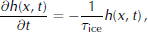
where τ ice = 250 years is used as the characteristic timescale for the ice to surge (Reference MacAyealMacAyeal, 1993a). The accumulation will be disregarded during the surge.
When the ice sheet thins, frictional heating is created due to a loss in gravitational potential energy. All gravitational potential energy is dissipated at the bed and its rate is independent of the horizontal position (Reference MacAyealMacAyeal, 1993a). The rate at which frictional heating occurs at the bed is therefore equal to the rate of change of the total gravitational potential energy stored in the ice sheet during the purge phase. Frictional heating is given by

since the total gravitational potential energy stored is equal to ρ g H2/2 and, according to Equation (16), dH/dt = −H/τ ice. ρ i and g are assumed to be constant.
During the purge phase we assume that the temperature at the bottom remains at the melting temperature of ice, since any excess from the heat conduction through the ice will be used for melting. We assume (Reference MacAyealMacAyeal, 1993a) that the water at the bed is drained. In this way we do not have to consider any stored energy later in the cycle.
The purge phase will occur as long as the basal temperature remains at the pressure-melting point. This is controlled by the balance between the geothermal heat flux, the release of the frictional heating and the heat conduction through the ice.
Results
The width of the ice sheet is determined using Equations (10) and (11), and the heat-transfer Equation (12) is solved using the boundary conditions Equations (13) and (14). The advection in the heat-transfer equation and the rate of change of the width of the ice sheet are governed by the mass balance. The elevation of the equilibrium line is related to the sea surface temperature through two parameters Φ and Ψ. These two parameters are adjusted such that the surges of the ice sheet coincide with the timing of the observed HE. The following constraints are used to estimate the values of the unknown parameters Φ and Ψ.
1. By 6 kyr bp the LIS had disappeared except at Baffin Island, Nunavut (Reference Lowe and WalkerLowe and Walker, 1997, p. 32).
2. The Heinrich events H1 to H6 are dated at around 15, 23, 29, 39, 47.5 and 65 kyr bp, respectively, on the ss09sea timescale (Reference BondBond and others, 1993; Reference JohnsenJohnsen and others, 2001; Reference HemmingHemming, 2004).
3. The LIS did not exist during the Eemian (Reference Boulton, Smith and MorlandLowe and Walker, 1997, p. 339).
We obtain the best fit to the above constraints using values of Φ = 55mK − 1 and Ψ = 2505 m. This implies that for each degree of warming, the elevation of the equilibrium line will increase by 55 m or decrease when cooling. For a sea surface temperature of 0 ˚ C, the elevation of the equilibrium line at the centre of the ice sheet will be at 2505 m. The values of Φ and Ψ are found by performing an extensive search in the model-parameter space. The simulation begins at 115 kyr bp, at the end of the Eemian period. The evolution of the elevation of the ice-sheet surface for these values of Φ and Ψ is shown in Figure 1b.
(a) The temperature history obtained from the GRIP ice core. (b) The evolution of the ice sheet using Φ = 55 and Ψ = 2505. (c) A simulation in which the sea surface temperature for driving the upper boundary condition for the heat-transfer equation is constant in time. The temperature at the LGM has been used. (d) A simulation using constant elevation of the equilibrium line and constant accumulation rate a(t) in Equation (9). The elevation of the equilibrium line and the accumulation rate is given by the LGM climate. All these simulations have been performed using N = 1. The vertical thick grey lines represent the approximate timing of the observed HE.

Since the simulated surges do not always occur with the same period, we find from the simulation that the internal oscillations in the ice sheet are modulated by the climatic signal. The climatic signal affects the evolution of the ice sheet in two ways. First, it controls the mass-balance distribution on the ice sheet. Second, it controls the ice-sheet surface temperature through the varying sea surface temperature.
To investigate the separate effects of these two climatic forcings, we structure two tests. First we perform a simulation using a time-independent sea surface temperature as means of controlling the upper boundary condition for the heat transfer equation. The sea surface temperature term in Equation (13) is assumed to be constant, with a value corresponding to the Last Glacial Maximum (LGM) climate. The elevation of the equilibrium line, however, still varies with the climatically driven sea surface temperature in Equation (5). The values of Φ and Ψ mentioned above are used and the results are presented in Figure 1c.
A second experiment is performed using a time-independent elevation of the equilibrium line and thus a mass balance dependent only on the elevation of the ice-sheet surface. Furthermore, the adjustment to the positive part of the mass balance due to varying accumulation rate at GRIP is also time-independent. This corresponds to a constant sea surface temperature in Equation (5), and a constant a(t) in Equation (9). The ice surface temperature as the upper boundary condition for the heat-transfer equation still varies with the sea surface temperature as determined from the GRIP ice core. The values of Φ and Ψ mentioned above are used once more. The result of the simulation is shown in Figure 1d.
The result of the full climatic forcing shown in Figure 1b indicates that there is generally good agreement between the timing of HE simulated by the model and the occurrence of observed HE. Furthermore, one can see that the ice sheet does disappear at the beginning of the Holocene. The timing of the simulated surges is shown in Table 1 together with the observed timing of HE, as well as the time spacing between simulated HE. In agreement with observations, our results
The timing of simulated HE compared to timing of observed HE; time between two consecutive simulated HE is listed in second column

show that the surges do not occur with equal time spacing. We understand this to be an indication of the internally driven oscillation of the ice sheet being affected by external climatic forcing. The observation that the time-dependent accumulation rate influences the internally driven oscillation is also supported by Reference PaynePayne (1995). Some features, however, are less in agreement with the observed evolution of the LIS. There is an additional HE between H5 and H6, and H2 is not recreated in the simulation. These discrepancies are probably due to the simplicity of the model.
For the simulation driven only by varying mass balance, the period between the surges has generally increased compared to the result of the full climatically driven evolution, as seen in Figure 1c. In this situation, the ice sheet is generally colder because of the time-independent cold sea surface temperature corresponding to the LGM climate. The ice sheet is affected by the cold temperature through the diffusion and the advection of the cold temperature from the ice-sheet surface but also because of the build-up of the ice sheet using generally colder ice. Another factor is high accumulation rates which are generally coupled with warmer temperatures; in this simulation an increase in the varying accumulation rate does not coincide with an increased temperature. This makes it harder for the basal temperature to reach pressure-melting temperature, i.e. to initiate the surge.
Figure 1d shows the result of the simulation using only climatically driven varying sea surface temperature. The strength of the surges, as well as the period between the surges, roughly follows a trend similar to the trend of the sea surface temperature. The first part of the glacial period, from about 115 kyr bp to 70 kyr bp, is generally warmer than the last part of the glacial period from about 70 kyr bp to 10 kyr bp. This results in shorter periods between the surges of the ice sheet in the first part compared to the last part of the glacial period. This is because warmer surface temperatures allow basal temperatures to reach the melting point faster, thus initiating a surge. In addition, since the accumulation rate caused by the climate at the LGM is low, there is less downward advection of cold ice from the surface which does not decrease the basal temperature significantly.
One of the main problems with simulating the LIS is lack of knowledge of the mass balance. By scaling Equation (8) with parameter N we have investigated what effect an increased and a decreased accumulation rate have on the timing of the surges. The results are shown in Figure 2. Using N = 1.5 is equivalent to having a 50% increase in accumulation rate, while using N = 0.5 is equivalent to having a 50% decrease in accumulation rate. The increase in accumulation rate results in shorter periods and stronger surges, while the decrease in accumulation rate has the opposite effect. The strength of the surges roughly follows the simulation for N = 1. Since the trend of the strength of the surges is roughly the same for all values of N, we suggest that the surge strength is mainly controlled by the temperature record. The reason for the shorter periods between surges using N = 1.5 is the effects of increased elevation and increased advection of cold surface temperatures, which influence the basal temperature and therefore the timing of surges. Increased thickness of the ice sheet has an isolating effect, which will increase the basal temperature. Increased downward advection, due to increased mass balance of cold ice from the surface of the ice sheet, will result in a lowering of the basal temperature.
The evolution of the ice sheet for different values of N, corresponding to different amounts of the positive part of the mass balance compared to the simulation presented in Figure 1b. Using N = 1.5 corresponds to a 50% increase in accumulation rate, while using N = 0.5 corresponds to a 50% decrease in accumulation rate.
As can be seen in Figure 2 using a value of N = 1.5, enhancing the accumulation rates also results in a faster growth of the ice sheet and therefore an increasing isolation effect. A thicker ice sheet will also result in an increased lowering of the pressure-dependent melting temperature. By contrast, a decrease in the accumulation rate from lower values of N shows that the period between the surges increases and the strength of the surges decreases.
Conclusions
Using a very simple combined ice-sheet and heat-flow model, we have attempted to tune the mass balance over the LIS during the glacial period in such a way that the ice sheet surged at approximately the same time as HE observed from the deep-sea sediment cores across the North Atlantic.
Driving the temperature and accumulation to change according to the reconstructed climate record from the GRIP ice core, the surges can be tuned to occur at approximately the correct time. We showed that changes in the driving temperature and accumulation histories do affect the development of the ice sheet as well as the internal temperatures. The amount of accumulation on the ice sheet plays an important role in its evolution.
The work of others (Reference MacAyealMacAyeal, 1993a; Reference PaynePayne, 1995; Reference Calov, Ganopolski, Petoukhov, Claussen and GreveCalov and others, 2002) has shown convincingly that the reason for the HE is to be found in a part of the basal region of the LIS reaching pressure-melting temperature. The basal region reaching the melting temperature then causes the ice sheet to begin to surge. The work presented here also favours this hypothesis: that surges of the LIS occur because the temperature at the bed reaches the melting temperature. We have shown that a varying glacial climate needs to be taken into account when simulating surges of the LIS, in order to properly simulate the observed HE. This conclusion is based upon our simulation using both the temperature and accumulation rate profile obtained from the GRIP ice core, as well as the simulations where only the ice-sheet surface temperature or the accumulation rate varies. We conclude that even a simple model, as used here, sheds light on the mechanism that caused the LIS to surge with irregular intervals, causing very significant climate changes in the North Atlantic during the glacial period.



