1 Introduction
Since the 1990s, global banks have actively engaged in cross-border lending, which has led to a dramatic increase in gross capital flows for both advanced and emerging economies. Rey (Reference Rey2018) and Miranda-Agrippino and Rey (Reference Miranda-Agrippino and Rey2020) find that a key determinant of the global financial cycle is US economic conditions which affects the rest of the world through financial linkages generated by global banks. The global financial cycle may not necessarily align with the cycle in individual emerging economies. For example, Cetorelli and Goldberg (Reference Cetorelli and Goldberg2011), Allen et al. (Reference Allen, Beck, Carletti, Lane, Schoenmaker and Wagner2011), and Takats (Reference Takats2010) document the drying-up of cross-border bank lending to emerging markets during the global financial crisis. Subsequently, cross-border credits to emerging markets rebounded quickly when the USA implemented quantitative easing and later on contracted due to the “taper tantrum.” How do emerging economies deal with the spillovers from external disturbances coming from major economies?
The majority of theoretical and empirical literature focuses on the spillover of US monetary conditions to emerging economies. This paper, instead, studies how financial risks from the USA propagate to emerging markets through global banks. Moreover, I explore to what extent emerging markets can use monetary and capital account policies to insulate themselves from these external disturbances.
I study the propagation of financial risk shocks for three reasons. First, a growing theoretical literature has demonstrated that risk or uncertainty shocks are an important driving force of the business cycle (e.g. Bloom (Reference Bloom2009), Christiano et al. (2014)). There is also evidence that volatility shocks in one economy have non-negligible impacts on other economies. For example, Fernandez-Villaverde et al. (2011) show that stochastic volatility in the world real interest rate has sizable effects on small open economies. However, the way in which risk shocks interact with the existence of global banks in an open economy context remains relatively unexplored. Second, Forbes and Warnock (Reference Forbes and Warnock2012) and Rey (Reference Rey2018) find strong empirical evidence that risk shocks in the USA can consistently explain gross capital flows. When US risk is low (high), cross-border flows surge (retrench). Last, Stock and Watson (Reference Stock and Watson2012) found empirical evidence that the 2008 global financial crisis was associated with large financial and uncertainty shocks. Footnote 1 The large weight of complex financial instruments in global bank’s balance sheets increased the volatility of their returns. The financial risk shocks modeled in this paper provide further evidence for this channel.
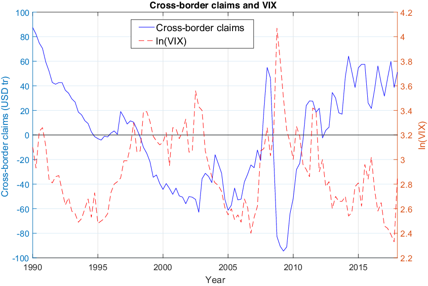
The data suggest a possible link between global financial stress and global bank lending to emerging markets. Figure 1 shows the time series of the log of the Chicago Board Options Exchange VIX index (in blue) and linearly detrended cross-border claims of US banks to emerging economies (in red). Footnote 2 Two periods of relatively high financial risk were the dot-com bubble in early 2000, and the global financial crisis in 2008. Both periods were associated with a retrenchment of cross-border claims to emerging economies. The sharp reversal of cross-border claims in 2008Q4 was particularly remarkable. The subsequent fall in financial risk and the quick rebound in claims might have been related to US quantitative easing. Overall, the empirical correlation between these two series is -0.35 and is statistically different from zero (at 5% confidence level). Appendix A provides a formal recursive structural vector autoregressive (VAR) analysis similar to Rey (Reference Rey2018) and Bruno and Shin (Reference Bruno and Shin2015) to study the relationships among US monetary policy, financial risk, and cross-border bank claims to emerging economies.
The VIX index and cross-border bank lending to emerging economies.

To explore the spillovers of financial shocks from the center to emerging market economies, I embed a stylized banking network with cross-border lending and financial frictions in an otherwise standard core–periphery dynamic stochastic general equilibrium (DSGE) model. The banking network is similar to Ueda (Reference Ueda2012), which in turn builds on the costly state verification (CSV) framework of Bernanke et al. (Reference Bernanke, Gertler, Gilchrist, Taylor and Woodford1999) (henceforth Bernanke, Gertler and Gilchrist (BGG)). Entrepreneurs in the center and the emerging economy borrow from global banks, and investors in the center indirectly lend to the entrepreneurs through global banks. These financial transactions are interpreted as bank lending in this framework because banks are specialists in monitoring financial transactions, which is consistent with the CSV framework. Furthermore, since banks borrow with much higher leverage than nonfinancial firms, the resulting chained credit contract [Hirakata et al. (Reference Hirakata, Sudo and Ueda2017)] creates larger amplifications than standard BGG (1999) contracts. Financial frictions driven by CSV lead to an endogenous wedge between firms’ expected return on capital and the risk-free interest rate, called the external finance premium. Financial risk is modeled as an increase in the dispersion of global banks’ idiosyncratic productivity, similar to Christiano et al. (2014). When financial risk in the global bank sector increases, investors in the center, the common lenders, require higher compensation in exchange for bearing heightened risk, which leads to a synchronized rise in the external finance premia in the center and the emerging economy. In a calibrated model, I show that this effect is important, resulting in a fall in investment and asset prices in the emerging market, consistent with the empirical observations during global financial cycles.
Using the structural model as a laboratory, I explore the welfare gains of using active monetary and capital account policy to insulate an emerging economy from external financial risks. First, I find that a peg creates excessive inflation and output volatility, which reduces welfare. Incorporating a global banking network does not overturn this result. Second, temporary capital controls improve welfare when there is cross-border bank lending. Capital controls in the form of a tax or subsidy help to stabilize capital flows, moderate the jump in the external finance premium, and support capital investment. Similar to Davis and Presno (Reference Davis and Presno2017) and Aoki et al. (Reference Aoki, Benigno and Kiytoaki2016), I find that capital controls mitigate the trade-off between macroeconomic and financial stability, so that monetary policy can focus on macroeconomic stability. Moreover, as capital controls impact the bank-lending channel directly, this policy improves welfare under fixed and flexible exchange rate regimes. Third, the effectiveness of capital controls increases with the degree of financial integration.
This paper is related to three strands of literature. The first studies the transmission of uncertainty or risk shocks to the macroeconomy (such as Bloom (Reference Bloom2009), Leduc and Liu (Reference Leduc and Liu2016)). In particular, Arellano et al. (Reference Arellano, Bai and Kehoe2018), Gilchrist et al. (Reference Gilchrist, Sim and ZakrajŠek2014) and Christiano et al. (2014) consider the interaction between uncertainty shocks and financial frictions and emphasize their amplification through a financial accelerator mechanism. A growing literature studies the role of uncertainty in an open economy context. Fernandez-Villaverde et al. (2011) find that stochastic volatility shocks in the real interest rate have sizeable effects on real activities in emerging economies in Latin America. In a similar vein, Mumtaz and Theodoridis (Reference Mumtaz and Theodoridis2015) show that a rise in volatility in the US economy leads to a decline in UK economic activity. Caggiano et al. (Reference Caggiano, Castelnuovo and Figueres2019), Colombo (Reference Colombo2013), Klosner and Sekkel (2014) and Luk et al. (Reference Luk, Cheng, Ng and Wong2020) estimate structural vector-autoregressive models and find significant spillover effects of uncertainty shocks from major economies (typically the USA) to the rest of the world.
A second strand of literature analyses the international transmission of shocks in a two-country open macro model with finan cial frictions. Footnote 3 My modeling framework builds on Kollmann et al. (Reference Kollmann, Enders and Muller2011), Kollmann (Reference Kollmann2013), Kalemli-Ozcan et al. (2013), and Ueda (Reference Ueda2012), which show that financial frictions in the global banking sector play an important role in the international business cycle. Devereux and Yetman (Reference Devereux and Yetman2010), Dedola and Lombardo (Reference Dedola and Lombardo2012), and Banerjee et al. (Reference Banerjee, Devereux and Lombardo2016) incorporate financial shocks as an exogenous tightening of collateral requirements and demonstrate that this shock gives rise to strong comovement of business cycles across countries. But this collateral-requirement shock does not account for a rise in uncertainty, a salient feature observed during crises.
The paper is also related to the global financial cycle and the “dilemma-trilemma” debate. Shin (Reference Shin2012), Rey (Reference Rey2018), and Miranda-Agrippino and Rey (Reference Miranda-Agrippino and Rey2020) argue for the “dilemma” view that international financial integration makes it harder for emerging economies to maintain macroeconomic stability, regardless of the exchange rate regime. Obstfeld (Reference Obstfeld, Raddatz, Saravia and Ventura2015) contends that financial integration reduces the effectiveness of monetary policy because it increases the burden carried by monetary policy. In relation to this view, Farhi and Werning (Reference Farhi and Werning2014), Schmitt-Grohe and Uribe (Reference Schmitt-Grohe and Uribe2012), and Liu and Spiegel (Reference Liu and Spiegel2015) explore the role of capital controls in small open economies. Aoki et al. (Reference Aoki, Benigno and Kiytoaki2016), Devereux et al. (Reference Devereux, Young and Yu2019), and Davis and Presno (Reference Davis and Presno2017) are closest in spirit to this paper. They discuss monetary policy and capital controls in small open economy models with credit frictions. However, they do not focus on the effects of financial risks.
The rest of the paper is organized as follows. The next section describes the setup of the banking network and derives the optimal contract for global banks subject to financial frictions. Section 3 embeds the banking network into a center-periphery DSGE model, and Section 4 discusses calibration issues. Section 5 discusses monetary policy shocks and financial risk shocks from the center. Section 6 explores different monetary and capital account policies for emerging economies. Section 7 concludes.
2 Chained Credit Contracts
I construct a two-country model with a center economy and an emerging economy. Each economy is populated by representative households, goods producing firms, and capital producing firms as in a standard New Keynesian model. In addition, there are investors, banks, and entrepreneurs in both economies who borrow and lend subject to financial frictions and an exogenous global banking network. The way that the global banking network is modeled is new. Relative to Ueda (Reference Ueda2012), we make four changes. First, we allow nominal loan contracts. Second, the two economies here are different in size, whereas the ones in Ueda (Reference Ueda2012) are symmetric. Third, in this model, only banks in the center economy can engage in cross-border lending, whereas in Ueda (Reference Ueda2012) all investors and banks can do so. Fourth, uncertainty shocks are analyzed as in Christiano et al. (2014) but are not considered in Ueda (Reference Ueda2012).
This section describes the CSV problems in financial markets and the resulting chained-credit contracts. It shows that, when global banks engage in cross-border lending, financial risk shocks in the center lead to a correlated rise in the external finance premium in both the center and emerging economy, consistent with what is observed during global financial cycles. This banking network is embedded in a standard two-country model in the next section.
2.1 Overview
The banking network is illustrated in Figure 2. There are two countries, Home and Foreign. The periphery emerging (home) economy is a small open economy of size
 $m \rightarrow 0$
, and the center (foreign) economy is of size
 $(1-m)$
. Each arrow in the figure stands for a lending contract. In each economy, investors lend to banks and banks lend to entrepreneurs. A crucial assumption is that entrepreneurs in the emerging economy borrow from both local banks and banks in the center, and so the banks in the center are called global banks.
Chained credit contract in a two-country model.

In the following, there are five types of loan contract labeled
 $i\in \{B, B*, E, E*, E\times \}$
. A “B” contract is one in which banks in the emerging economy borrow from local investors; a “E” contract is one in which entrepreneurs in the emerging economy borrow from local banks. “
 $B*$
” and “
 $E*$
” contracts are analogous for the center, which go through global banks. Lastly, an “
 $E\times$
” contract is a cross-border loan contract between global banks and entrepreneurs in the emerging economy.
Footnote 4
In each of the five types of contract, we assume that a lender lends to an infinite number of borrowers.
Footnote 5
Each of the five types of loan contract is subject to financial frictions because lenders face a CSV problem identical to BGG (1999). Each borrower’s return on investment faces an idiosyncratic shock
 $\omega^{i}$
drawn from the distribution
 $\log(\omega^{i})\sim N(-0.5(s^{i})^{2},(s^{i})^{2})$
, where
 $E(\omega^{i})=1$
and the cumulative density function is
 $F^{i} (\omega^{i})$
.
Footnote 6 Only the borrower in a loan contract can observe his own idiosyncratic shock costlessly. To find out the realization of the idiosyncratic shock for a specific borrower, the lender needs to pay monitoring costs, assumed to be a constant fraction
 $\mu^{i}$
of the revenue of the borrower.
Townsend (Reference Townsend1979) shows that as a result of the CSV problem, the lender does not monitor when the borrower’s draw of the shock is above a cutoff value
 $\tilde{\omega}^{i}$
. The borrower repays the lender with an agreed state-contingent contractual interest rate
 $Z^{i}$
and retains what remains. When the borrower’s draw is below the cutoff value, the borrower is bankrupt, the lender monitors and takes whatever remains from the bankrupt borrower. A loan contract then decides how the revenue is split between the borrower and lender. To see this, suppose a borrower in contract i borrows an amount
 $b^{i}$
, and his return on investment before the idiosyncratic shock is realized is given by
 $roi^{i}$
, then the cutoff value of idiosyncratic shock
 $\tilde{\omega}^{i}$
is defined by:
 \begin{equation}Z^{i}b^{i} = \tilde{\omega}^{i} roi^{i}. \end{equation}
Then the lender receives the expected revenue (before monitoring) given by:
 \begin{eqnarray*} \int_{0}^{\tilde{\omega}^{i}} \omega^{i} roi^{i} dF^{i} + \int_{\tilde{\omega}^{i}}^{\infty} Z^{i}b^{i} dF^{i}= \Gamma^{i}(\tilde{\omega}^{i}) roi^{i},\end{eqnarray*}
where
 $\Gamma^{i}(\tilde{\omega}^{i})$
is the share of the total revenue that goes to the lender (before monitoring), given by:
 \begin{equation}\Gamma^{i}(\tilde{\omega}^{i}) \equiv G^{i}(\tilde{\omega}^{i}) +[1-F^{i}(\tilde{\omega}^{i})]\tilde{\omega}^{i}, \end{equation}
where
 $G^{i}(\tilde{\omega}^{i}) \equiv \int_{0}^{\tilde{\omega}^{i}}\omega^{i} dF^{i}(\omega^{i})$
accounts for what the lender gets on average (before monitoring occurs) if the borrower defaults, and
 $[1-F^{i}(\tilde{\omega}^{i})]\tilde{\omega}^{i}$
accounts for the payment when
 $\omega^{i}\geq \tilde{\omega}^{i}$
and the borrower does not default. Note that
 $F^{i}, G^{i}, \Gamma^{i}$
depend also on
 $s^{i}$
which measures the cross-sectional dispersion of risk, but I suppress
 $s^{i}$
for simplicity.
In the following, I discuss the details of the cashflow among investors, banks, and entrepreneurs as well as the optimal contracting problems faced by the banks. Hirakata et al. (Reference Hirakata, Sudo and Ueda2017) show that the solution to this optimal contracting problem is one in which the capital to net worth ratio is equalized within banks and within entrepreneurs, so one only needs to keep track of the aggregate quantities. For this reason, in the discussion below, entrepreneurs and banks of the same type are treated as a single agent.
2.2 Entrepreneurs
Entrepreneurs in the emerging economy have total net worth
 $N_{t}^{E}$
at the beginning of a period. They borrow
 $B_{Ht}$
units of nominal debt from local banks and and
 $B_{Ht}^{*}$
units of nominal debt from global banks to finance their purchase of capital
 $K_{t}$
at a (real) price
 $Q_{t}$
, receiving an average return of
 $R_{t+1}^{E}Q_{t}K_{t}$
. The balance sheet is then given by:
 \begin{equation}Q_{t}K_{t} = N_{t}^{E} + \frac{B_{Ht}}{P_{t}} + \frac{B_{Ht}^{*} \mathscr{E}_{t}}{P_{t}},\end{equation}
where
 $\mathscr{E}_{t}$
is the nominal exchange rate, defined as the price of home currency in terms of foreign currency, and
 $P_{t}$
is the price level in the emerging economy.
I follow Ueda (Reference Ueda2012) to abstract from the portfolio choice decision by assuming that a fraction
 $(1-\eta)$
of debt comes from a local bank and the remaining fraction
 $\eta$
from a global bank, where
 $\eta$
is an exogenous parameter capturing the emerging economy’s openness to cross-border lending, or the degree of financial integration.
Footnote 7
This means that
 $\frac{B_{Ht}}{P_{t}} = (1-\eta) (Q_{t}K_{Ht} -N_{t}^{E})$
, and
 $\frac{B_{Ht}^{*} \mathscr{E}_{t}}{P_{t}} = \eta (Q_{t}K_{Ft} -N_{t}^{E})$
, where
 $K_{t} =(1-\eta) K_{Ht} + \eta K_{Ft}$
. In Section 5, I will study the effect of financial integration by adjusting the value of
 $\eta$
.
Entrepreneurs in the center have total net worth
 $N^{E*}_{t}$
at the beginning of a given period. They only borrow from global banks to purchase capital
 $K_{t}^{*}$
at a price
 $Q_{t}^{*}$
, which earns an average return
 $R_{t+1}^{E*}Q_{t}^{*}K_{t}^{*}$
.
2.3 Global Banks
Global banks are located in the center. They borrow from investors in the center and lend to entrepreneurs in both the center and the emerging economy. The (real) total lending by global banks
 $X_{t}^{*}$
is given by:
 \begin{equation}X_{t}^{*} \equiv \frac{m}{1-m}\eta \frac{\left(Q_{t}K_{Ft}- N_{t}^{E}\right)}{S_{t}} + \left(Q_{t}^{*}K_{t}^{*}- N_{t}^{E*}\right),\end{equation}
where
 $S_{t} \equiv \mathscr{E}_{t}P_{t}^{*}/P_{t}$
is the real exchange rate. The first term denotes aggregate lending by global banks to entrepreneurs in the emerging economy using
 $E\times$
contracts, and the second term denotes aggregate lending by global banks to entrepreneurs in the center using
 $E*$
contracts.
The average (real) revenue of global banks’ lending, denoted as
 $R^{B*}_{t}X^{*}_{t-1}$
, is given by:
 \begin{eqnarray}R^{B*}_{t} X^{*}_{t-1} &=& \frac{m}{1-m} \eta \frac{\left[\Gamma^{E\times}\left(\tilde{\omega}^{E\times}_{t}\right) - \mu^{E\times} G^{E\times}\left(\tilde{\omega}^{E\times}_{t}\right)\right] R^{E}_{t} Q_{t-1} K_{Ft-1}}{S_{t}} \nonumber \\&&+ \left[\Gamma^{E*}\left(\tilde{\omega}^{E*}_{t}\right) - \mu^{E*}G^{E*}\left(\tilde{\omega}^{E*}_{t}\right) \right] R^{E*}_{t}Q^{*}_{t-1}K^{*}_{t-1}. \end{eqnarray}
The first term on the right-hand side is the gross revenue made by entrepreneurs in the emerging economy, where the term
 $(\Gamma^{E\times} - \mu^{E\times} G^{E\times})$
accounts for the share of revenue going to global banks after monitoring costs are paid. In other words, this is the repayment by home entrepreneurs to global banks. Analogously, the second term refers to the repayment by the entrepreneurs from the center to global banks.
Global banks have aggregate net worth
 $N_{t}^{B*}$
and borrow
 $(X_{t}^{*}-N_{t}^{B*})$
from investors in the center. The return on banking activity is subject to an idiosyncratic shock,
 $\omega_{t+1}^{B*}$
. They are subject to the participation constraints of entrepreneurs in the center and the emerging economy in each
 $t+1$
state of nature:
 \begin{eqnarray}\eta R^{E}_{t+1}Q_{t}K_{Ft} \left[1-\Gamma^{E\times} \left(\tilde{\omega}^{E\times}_{t+1}\right)\right] &\geq& \eta R^{E}_{t+1}N^{E}_{t}, \end{eqnarray}
 \begin{eqnarray}R^{E*}_{t+1} Q^{*}_{t}K^{*}_{t} \left[1-\Gamma^{E*} \left(\tilde{\omega}^{E*}_{t+1}\right)\right] &\geq& R^{E*}_{t+1}N^{E*}_{t}. \end{eqnarray}
Equation (6) is the participation constraint of the entrepreneurs in the emerging economy. Note that the left-hand side is the share of revenue that goes to the entrepreneur (a share of
 $(1-\Gamma^{E\times} )$
). One interpretation of this equation is that global banks have market power, so when an entrepreneur wants to increase his credit, the bank will raise the contractual interest rate accordingly (and so the cutoff threshold, due to (1)), so that the entrepreneur is as well off as self-financing. Equation (7) is an analogous participation constraint for the entrepreneurs in the center.
Moreover, global banks are subject to the participation constraint of investors in the center in each
 $t+1$
state of nature:
 \begin{eqnarray}\left[\Gamma^{B*}\left(\tilde{\omega}^{B*}_{t+1}\right)- \mu^{B*} G^{B*}\left(\tilde{\omega}^{B*}_{t+1}\right)\right] R^{B*}_{t+1} X^{*}_{t} &\geq& R^{*}_{t} \left(X^{*}_{t}- N^{B*}_{t}\right). \end{eqnarray}
Equation (8) ensures that the return received by investors, represented by the left-hand side of the equation, is as high as the risk-free return.
Global banks choose the amount of lending to entrepreneurs in the center and the emerging market (which is equivalent to choosing
 $\{K^{*}_{t}, K_{Ft}\}$
), and the contractual interest rates of the three contracts (which, given the one-to-one correspondence between
 $Z^{i}$
and
 $\tilde{\omega}^{i}$
shown in (1), is equivalent to choosing
 $\{\tilde{\omega}^{B*}_{t+1},\tilde{\omega}^{E\times}_{t+1},\tilde{\omega}^{E*}_{t+1}\}$
) to maximize their expected profit function:
 \begin{eqnarray*} E_{t} \left[1-\Gamma^{B*}\left(\tilde{\omega}^{B*}_{t+1}\right) \right] R^{B*}_{t+1} X_{t}^{*},\end{eqnarray*}
subject to constraints (6), (7), and (8). Footnote 8
The following proposition states the solution to the optimal financial contracting problem of the global banks: Footnote 9
PROPOSITION 1 Up to the first-order approximation, the first-order conditions associated with the global bank’s optimization problem arepro1
 \begin{eqnarray} E_{t}\left( \frac{R_{t+1}^{E*}}{R_{t}^{*}} \right) &=& E_{t} \left[ \rho^{B*}\left(\tilde{\omega}_{t+1}^{B*}; s_{t}^{B*}\right) \times \rho^{E*}\left(\tilde{\omega}_{t+1}^{E*}; s_{t}^{E*}\right) \right], \end{eqnarray}
 \begin{eqnarray} E_{t}\left( \frac{R_{t+1}^{E}}{R_{t}} \right) &=& E_{t} \left[ \rho^{B*}\left(\tilde{\omega}_{t+1}^{B*}; s_{t}^{B*}\right) \times \rho^{E\times}\left(\tilde{\omega}_{t+1}^{E\times}; s_{t}^{E\times}\right) \right], \quad \text{for}\quad \eta >0, \end{eqnarray}
where the function
 $\rho^{i}(\tilde{\omega}^{i}; s^{i}) \geq 1$
is given in Appendix B. Furthermore,
 \begin{equation*} \frac{\partial \rho^{i}(\tilde{\omega}^{i}; s^{i})}{\partial \tilde{\omega}^{i}}>0, \;\; \frac{\partial \rho^{i}(\tilde{\omega}^{i}; s^{i})}{\partial s^{i}}>0.\end{equation*}
Consider the demand for credit in the center (9) first. It states that an exogenous rise in the external finance premium,
 $E_{t}(R_{t+1}^{E*})/R_{t}^{*}$
, leads to an increase in the default threshold for global banks,
 $\tilde{\omega}_{t+1}^{B*}$
, or an increase in the default threshold for foreign entrepreneurs,
 $\tilde{\omega}_{t+1}^{E*}$
, or both. Borrowers subject to a CSV problem have a risk-shifting incentive: when a borrower receives an unfavorable idiosyncratic shock and defaults, she does not care about how much she owes the lender; on the other hand, if she can repay the prespecified amount, she pockets the upside profit. As a result, when the external finance premium rises exogenously, the expected return increases and entrepreneurs have an incentive to increase their capital investment. For given net worth, either banks or entrepreneurs have to increase their credit, but this leads to higher default probability in either the
 $E*$
contract or the
 $B*$
contract, so the cutoff thresholds rise because lenders need to break even. (Note that the right-hand side of the first-order condition can be factorized into two
 $\rho$
terms related to the two subcontracts. This derivation is new relative to Hirakata et al. (Reference Hirakata, Sudo and Ueda2017) and corresponds to the intuition above.)
In equilibrium, the external finance premium is weakly greater than unity because lenders expect resources to be lost through monitoring, which are compensated by an external finance premium. Other things equal, a rise in the cutoff value
 $\tilde{\omega}_{t+1}^{i}$
implies an increase in defaults, so the external finance premium is increasing in the cutoff value. Furthermore,
 $\rho^{i}_{s}>0$
because a more dispersed distribution of idiosyncratic shock means more expected defaults, so higher external finance premium is needed.
The optimal cross-border lending decision, (10)1, has a similar interpretation. When entrepreneurs in the emerging economy borrow from global banks (
 $\eta > 0$
), the external finance premium for entrepreneurs in the emerging economy,
 $E_{t}(R^{E}_{t+1})/R_{t}$
, can also be factored into two components,
 $\rho^{B*}$
and
 $\rho^{E\times}$
, which correspond to lending by investors in the center to global banks and cross-border lending from global banks to entrepreneurs in the emerging economy.
As global banks borrow from investors in the center and are lenders to both center and emerging market entrepreneurs, the factor
 $\rho^{B*}$
appears in both (9) and (10)1. Since
 $\rho^{B*}_{s}>0$
, a rise in cross-sectional risk to global banks
 $s^{B*}$
increases their default probability and the monitoring costs faced by investors in the center. To compensate for higher monitoring costs, investors in the center require a higher external finance premia in the center and emerging economy simultaneously. This common lender effect is identified by Ueda (Reference Ueda2012). In the subsequent simulation exercise I focus on the shock
 $s^{B*}_{t}$
, which follows an exogenous AR(1) process: (For simplicity, dispersions of other idiosyncratic shocks are constant.)
 \begin{equation}\ln s^{B*}_{t} = (1-\lambda^{B*}) \ln \bar{s}^{B*} + \lambda^{B*}\ln s^{B*}_{t-1} + \epsilon^{B*}_{t},\end{equation}
where
 $\bar{s}^{B*}$
is the steady-state value of
 $s^{B*}_{t}$
, and
 $\epsilon^{B*}_{t} \stackrel{i.i.d}{\sim} N (0,(\sigma^{B*}_{t-1})^{2} )$
. This shock is similar to Christiano et al. (2014) which refers to a shock to the cross-sectional dispersion of productivity as a risk shock. Here, the shock increases the cross-sectional dispersion of global bank productivity, so I refer it as a financial risk shock.
2.4 Local Banks
Banks in the emerging economy borrow locally and lend to local entrepreneurs. They are subject to the same CSV friction as global banks but do not engage in cross-border lending. This assumption allows me to focus on the effect of cross-border bank lending. They solve a profit maximization problem subject to the chained credit contract structure similar to the one faced by global banks. The first-order condition is given by: Footnote 10
 \begin{eqnarray} E_{t} \left(\frac{R^{E}_{t+1}}{R_{t}}\right) &=& E_{t} \left[ \rho^{B}\left(\tilde{\omega}^{B}_{t+1}; s^{B}_{t+1}\right) \times \rho^{E}\left(\tilde{\omega}^{E}_{t+1}; s^{E}_{t+1}\right) \right]. \end{eqnarray}
3. THE REST OF THE MODEL
This section describes the rest of the two-country model, which is standard. The production part closely follows BGG (1999) and Ueda (Reference Ueda2012) and the open economy part follows Gali and Monacelli (Reference Gali and Monacelli2005). I assume that the two economies have identical preferences, technology, and market structure apart from what is specified in the chained credit contracts. In the following, I do not write out equations for the center when they are analogous to the ones for the emerging economy.
3.1 Aggregate Quantities
Final goods for consumption
 $C_{t}$
, investment
 $I_{t}$
, and wasted resources due to monitoring in the financial contracts are Cobb–Douglas composites of center and periphery goods. Define variables
 $M = \{ C, I, MonCost \}$
as:
 \begin{equation} M_{t} = \frac{ M_{Ht}^{\nu} M_{Ft}^{1-\nu} }{\nu^{\nu} (1-\nu)^{1-\nu}}.\end{equation}
where the subscript H(F) denote goods produced in the emerging economy (center). The weight of imported goods in the good baset is denoted as
 $(1-\nu)$
and
 $(1-\nu)$
is given by
 $(1-\nu) \equiv (1-m) \zeta$
, where
 $\zeta$
is the trade openness. Similarly, households in the center have the following aggregator:
 \begin{equation} M^{*}_{t} = \frac{(M_{Ht}^{*})^{1-\nu^{*}}(M_{Ft}^{*})^{\nu^{*}}}{(\nu^{*})^{\nu^{*}} (1-\nu^{*})^{1-\nu^{*}}},\end{equation}
where
 $(1-\nu^{*}) = m \zeta^{*}$
. I follow Faia and Monacelli (Reference Faia and Monacelli2008) to restrict my attention to preferences that show a symmetric degree of home bias across countries such that
 $\zeta = \zeta^{*}$
. The corresponding price indices are given by
 $P_{t} = P_{Ht}^{\nu} P_{Ft}^{1-\nu}, \;\; P^{*}_{t} =(P^{*}_{Ht})^{1-\nu^{*}}(P^{*}_{Ft})^{\nu^{*}}$
.
I use
 $T_{t}$
to denote the terms of trade so that
 $T_{t}\equiv P_{Ft}/ P_{Ht}$
. Assuming that the law of one price holds across each variety of goods, then
 $P_{Ft} = \mathscr{E}_{t} P_{Ft}^{*}$
. Note that the real exchange rate
 $S_{t} = T_{t}^{\nu + \nu^{*}-1}$
is increasing in the terms of trade.
3.2 Households
A representative household in the emerging economy consumes, supplies labor, and saves. The household maximizes the following utility:
 \begin{equation} U_{0} = E_{0} \sum_{t=0}^{\infty} \beta^{t} u(C_{t}, L_{Ct}), \end{equation}
where
 $C_{t}$
is the consumption aggregate and
 $L_{Ct}$
is the labor supplied by the representative household. Utility is assumed to be additively separable:
 \begin{equation*} u(C_{t}, L_{Ct}) = \ln C_{t} - \chi \frac{L_{Ct}^{1+\varphi}}{1+\varphi}.\end{equation*}
Households are subject to the following budget constraint:
 \begin{equation} P_{t}C_{t} + D_{t+1} = w_{Ct}P_{t}L_{Ct} + R_{t}^{N} D_{t} + tr_{t},\end{equation}
where
 $D_{t+1}$
is the payoff in period
 $t+1$
of the portfolio held at the end of period t,
 $w_{Ct}$
is the real wage for the household, and
 $tr_{t}$
denotes transfers.
 $R_{t}^{N}$
is the nominal interest rate. The usual transversality condition applies. The intratemporal labor supply condition and the consumption Euler equation are given by the following:
 \begin{eqnarray} -\frac{u_{Lt}}{u_{Ct}} &=& w_{Ct}, \end{eqnarray}
 \begin{eqnarray} 1 &=& \beta R_{t}^{N} E_{t} \left[\left( \frac{u_{Ct+1}}{u_{Ct}} \right) \frac{P_{t}}{P_{t+1}}\right],\end{eqnarray}
where
 $u_{C}$
and
 $u_{L}$
denote marginal utility of consumption and marginal disutiltiy of labor, respectively. Household savings are channeled to risk-neutral investors who lend to the banks.
3.3 Goods Producers
A final goods producer in each economy aggregates a continuum of intermediate goods
 $j\in[0,1]$
using a Dixit–Stiglitz aggregator,
 $Y_{t} = (\int_{0}^{1} Y_{t}(j)^{\frac{\epsilon-1}{\epsilon}} dj )^{\frac{\epsilon}{\epsilon-1}}$
, and the demand for each type of good is
 $Y_{t}(j) = [ \frac{P_{Ht}(j)}{P_{Ht}}]^{-\epsilon} Y_{t}$
, where
 $P_{Ht} \equiv [ \int^{1}_{0} P_{Ht}(j)^{1-\epsilon}dj ]^{\frac{1}{1-\epsilon}}$
.
Intermediate goods producers
 $j\in[0,1]$
are monopolistically competitive. Each produces a good variety with capital and aggregate labor as inputs:
 \begin{equation} Y_{t}(j) = [K_{t-1}(j)]^{\alpha} [L_{t}(j)]^{1-\alpha}, \end{equation}
where aggregate labor is supplied by households, entrepreneurs, and bankers, given by
 $L_{t}(j) = [L_{Ct}(j)]^{1-\Omega_{B}-\Omega_{E}}[L_{Bt}(j)]^{\Omega_{B}}[L_{Et}(j)]^{\Omega_{E}}$
. Intermediate goods producers choose capital and labor inputs taking wages and the rental rate
 $r_{t}^{K}$
as given. Moreover, they set prices subject to nominal rigidities a la Calvo (Reference Calvo1983). Specifically, with probability
 $(1-\kappa)$
a firm resets its price optimally in a given period; otherwise, the firm’s price is fixed. Intermediate goods producers maximize their discounted stream of profits, given by:
 \begin{equation*} E_{t}\sum_{v=0}^{\infty} (\beta\kappa)^{v} \frac{u_{Ct+v}}{u_{Ct}}\frac{P_{t}}{P_{t+v}} \left\{ [P_{Ht}(j) - (1-\varrho) P_{t+v}MC_{t+v}(j)]Y_{t+v}(j) \right\},\end{equation*}
subject to the production function (19)1 and the demand function for each goods variety, where
 \begin{equation*}MC_{t}(j) = T_{t}^{1-\nu} \frac{\left(r_{t}^{K}\right)^{\alpha} \left[ (w_{Ct})^{(1-\Omega_{B}- \Omega_{E})}(w_{Bt})^{\Omega_{B}}(w_{Et})^{\Omega_{E}} \right]^{1-\alpha}}{\alpha^{\alpha}\left[(1-\Omega_{B}- \Omega_{E})^{(1-\Omega_{B}- \Omega_{E})}\Omega_{B}^{\Omega_{B}}\Omega_{E}^{\Omega_{E}}(1-\alpha)\right]^{1-\alpha}} \equiv MC_{t}\end{equation*}
is the real marginal cost, and
 $ \varrho = \epsilon^{-1}$
is a government subsidy which ensures that the steady state of the system with nominal rigidities is efficient.
All intermediate goods producers who reset their prices choose the same optimal price, denoted as
 $P^{opt}_{Ht}$
. Define
 $p^{opt}_{Ht} \equiv P^{opt}_{Ht}/P_{Ht}$
, then it follows that:
 \begin{equation} p^{opt}_{Ht} = \frac{E_{t}\sum_{v=0}^{\infty} (\beta\kappa)^{v} u_{Ct+v} \left( \frac{P_{Ht}}{P_{Ht+v}}\right)^{-\epsilon} MC_{t+v} Y_{t+v} T_{t+v}^{-(1-\nu)}}{E_{t}\sum_{v=0}^{\infty} (\beta\kappa)^{v} u_{Ct+v} \left( \frac{P_{Ht}}{P_{Ht+v}}\right)^{1-\epsilon} Y_{t+v} T_{t+v}^{-(1-\nu)}}.\end{equation}
The evolution of the price level is given by:
 \begin{equation} 1 = (1-\kappa) \left(p^{opt}_{Ht}\right)^{1-\epsilon} + \kappa \left( \frac{P_{Ht}}{P_{Ht-1}}\right)^{-(1-\epsilon)}. \end{equation}
3.4 Capital Goods Producers
A representative capital goods producer buys previously installed capital and combines with investments good
 $I_{t}$
from final goods producers to produce new capital.
Footnote 11
Newly produced capital is sold back to the entrepreneurs within the same period. Production of new capital is subject to convex investment adjustment costs. The evolution of capital is given by:
 \begin{equation} K_{t} = (1-\delta) K_{t-1} + ( 1- Adj_{t})I_{t},\end{equation}
where
 $Adj_{t} \equiv 0.5\psi^{I} \left( I_{t}/I_{t-1} - 1 \right)^{2}$
. Capital goods producers maximize their discounted future profit
 $E_{t} \!\sum_{v=0}^{\infty} \beta^{v} \frac{u_{Ct+v}}{u_{Ct}} \Pi_{t+v}^{K}$
where
 $\Pi_{t}^{K}{=}\, Q_{t} [K_{t} - (1-\delta) K_{t-1}]\,{-}\,I_{t}$
. The first-order condition for the optimal investment choice is
 \begin{eqnarray} 1 &=& Q_{t} \left[ 1- Adj_{t} - \psi^{I} \frac{I_{t}}{I_{t-1}} \left( \frac{I_{t}}{I_{t-1}}-1\right) \right]\nonumber\\&& + \beta E_{t} \left[ \frac{u_{Ct+1}}{u_{Ct}} Q_{t+1} \psi^{I} \left(\frac{I_{t+1}}{I_{t}}\right)^{2} \left( \frac{I_{t+1}}{I_{t}}-1\right) \right].\end{eqnarray}
3.5 Evolution of Net Worth
Banks and entrepreneurs accumulate their net worth each period. To prevent them from growing indefinitely, I follow BGG (1999) and assume that in each period an exogenous fraction
 $\gamma^{B}$
of banks and
 $\gamma^{E}$
of entrepreneurs survive and these fractions are the same across the two economies. New banks and entrepreneurs enter in each period to keep the number of banks and entrepreneurs unchanged over time. Assume that bankers and entrepreneurs supply inelastically one unit of labor
 $(L_{Bt}=L_{Et} = 1$
) to the goods producing firms and receive labor income, so newly joined bankers and entrepreneurs have positive net worth to start their business.
Entrepreneurial net worth evolves according to the following laws of motion:
 \begin{equation} N_{t}^{E} = \gamma^{E} R^{E}_{t} N_{t-1}^{E} + w_{Et}, \qquad N_{t}^{E*} = \gamma^{E} R^{E*}_{t} N_{t-1}^{E*} + w^{*}_{Et}.\end{equation}
The first term is the revenue retained by surviving entrepreneurs, and the second term is the wage income. Similarly, the net worth of banks in the emerging economy evolves as follows:
 \begin{align} N_{t}^{B} &= \gamma^{B} \left[ 1-\Gamma^{B}\left(\tilde{\omega}^{B}_{t}\right) \right] R_{t}^{B}X_{t-1} + w_{Bt},\nonumber\\[3pt] N_{t}^{B*} &= \gamma^{B} \left[ 1-\Gamma^{B*}\left(\tilde{\omega}^{B*}_{t}\right)\right] R_{t}^{B*}X^{*}_{t-1} + w^{*}_{Bt}.\end{align}
Finally, goods are wasted in the process of monitoring in the chained credit contracts. The monitoring costs are given by:
 \begin{eqnarray} {\textit{Moncost}}_{t} &=& (1-\eta)\mu^{E} G^{E}\left(\tilde{\omega}_{t}^{E}\right) R_{Ht}^{E} Q_{t-1}K_{Ht-1} + \mu^{B} G^{B}\left(\tilde{\omega}^{B}_{t}\right) R_{t}^{B} X_{t-1}, \end{eqnarray}
 \begin{eqnarray}{\textit{Moncost}}^{*}_{t} &=& \frac{m}{1-m}\eta \mu^{E\times} G^{E\times}\left(\tilde{\omega}^{E\times}_{t}\right) R^{E}_{t} \frac{Q_{t-1}K_{Ft-1}}{S_{t}} + \mu^{E*} G^{E*}\left(\tilde{\omega}^{E*}_{t}\right)R^{E*}_{t} Q_{t-1}^{*}K_{t-1}^{*} \nonumber\\ && + \mu^{B*} G^{B*}\left(\tilde{\omega}^{B*}_{t}\right) R^{B*}_{t} X_{t-1}^{*}.\end{eqnarray}
3.6 Market Clearing
Goods markets clear. Goods are consumed, invested, and wasted in the monitoring of failing banks and entrepreneurs. Therefore, for
 $M = \{ C, I, {\textit{MonCost}} \}$
:
 \begin{eqnarray} mY_{t} &=& m \sum_{M} M_{Ht} + (1-m) \sum_{M} M_{Ht}^{*}.\end{eqnarray}
3.7 Central Bank
The center sets the nominal interest rate according to the following monetary policy rule:
 \begin{eqnarray} R^{N*}_{t} &=& \beta^{-1} \left( \frac{\Pi_{Ft}^{*}}{\bar{\Pi}_{F}^{*}}\right)^{\phi_{\pi *}} \left( \frac{Y_{t}^{*}}{\bar{Y}^{*}}\right)^{\phi_{Y *}} e^{\epsilon_{R^{*}t}},\end{eqnarray}
where
 $\Pi^{*}_{Ft}\equiv P_{Ft}^{*}/P_{Ft-1}^{*}$
denotes producer price index inflation, and
 $\epsilon_{R^{*}t}$
is an i.i.d shock. As the center is large, its monetary policy does not react to prices and quantities in the emerging economy.
The emerging economy sets its nominal interest rate with the following rule:
 \begin{eqnarray} R^{N}_{t} &=& \beta^{-1} \left( \frac{\Pi_{Ht}}{\bar{\Pi}_{H}}\right)^{\phi_{\pi}} \left( \frac{Y_{t}}{\bar{Y}}\right)^{\phi_{Y}} \left( \frac{\mathscr{E}_{t}}{\mathscr{E}_{t-1}}\right)^{\phi_{\mathscr{E}}}, \end{eqnarray}
where
 $\Pi_{Ht} \equiv P_{Ht}/P_{Ht-1}$
, and the coefficients
 $\phi_{\pi}$
,
 $\phi_{Y}$
, and
 $\phi_{\mathscr{E}}$
denote inflation, output, and exchange rate sensitivities to the policy rate. The small open economy is assumed to use a general form of the interest rate rule which nests flexible
 $(\phi_{\mathscr{E}}=0)$
and fixed
 $(\phi_{\mathscr{E}} \rightarrow \infty)$
exchange rate regimes. We will examine various combination of sensitivity parameters
 $\{\phi_{\pi}, \phi_{Y}, \phi_{\mathscr{E}}\}$
in the emerging economy in the following sections.
4 Calibration
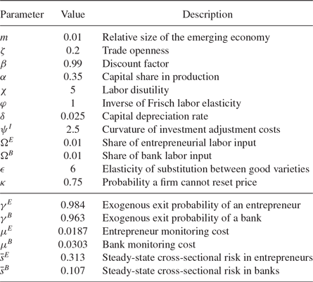
This section discusses the calibration of the model. Parameter values are summarized in Table 1. Each period is a quarter. The discount factor is
 $\beta = 0.99$
which implies that the steady-state interest rate is around
 $4.2\%$
per year. The relative size of the emerging economy, m, is set to
 $0.01$
to ensure that it does not have any observable effect on the center. I set the degree of trade openness at
 $\zeta=0.2$
, following De Paoli (Reference De Paoli2009). This implies
 $\nu = 0.802$
and
 $\nu^{*} = 0.998$
. The inverse of the Frisch elasticity of labor supply is set to
 $\varphi=1$
, following the estimate of Kimball and Shapiro (Reference Kimball and Shapiro2008). The labor disutility parameter is
 $\chi=5$
, so steady-state labor is normalized to around
 $0.4$
. Capital depreciation is
 $\delta=0.025$
. The curvature of the investment adjustment cost function,
 $\psi^{I}$
, is set to
 $2.5$
. The elasticity of substitution between goods varieties is set to
 $\epsilon=6$
, corresponding to a steady-state mark-up of 20%. The price stickiness parameter is
 $\kappa = 0.75$
. This value implies on average prices adjust once a year, which is supported by some micro data in Alvarez et al. (2006). The capital share in the production function is
 $\alpha = 0.35$
. I set
 $\Omega^{B} = \Omega^{E} = 0.01$
as in Hirakata et al. (Reference Hirakata, Sudo and Ueda2017), which ensures labor supply by bankers and entrepreneurs do not affect model dynamics.
Calibrated parameters

As there are five types of financial contracts in the system, many credit parameters need to be calibrated. To reduce the number of free parameters, I limit the differences between the two economies to their size and financial network structure, by making the following restrictions:
 \begin{eqnarray*} \mu^{B} = \mu^{B*}, \;\; \mu^{E} = \mu^{E\times} = \mu^{E*}, \\ \bar{s}^{B} = \bar{s}^{B*}, \;\; \bar{s}^{E} = \bar{s}^{E\times} = \bar{s}^{E*}.\end{eqnarray*}
Credit contract parameters
 $\{\mu^{E}, \mu^{B}, \bar{s}^{E}, \bar{s}^{B}, \gamma^{B}, \gamma^{E} \}$
are calibrated to match six targets in the symmetric system with no financial integration (i.e.
 $\eta =0$
). First, the annualized bank default probability is 2%. Second, the annualized entrepreneur default probability is also 2%. These two targets are the same as in Ueda (Reference Ueda2012), whereas BGG (1999) use a slightly higher target of 3%. Third, the entrepreneur capital to net worth ratio (
 $\bar{Q}\bar{K}/\bar{N}^{E}$
) is set to 2, a commonly used value in the literature. Fourth, the bank capital to net worth ratio (
 $\bar{Q}\bar{K}/\bar{N}^{B}$
) is set to 10, based on US Flow of Funds data.
Footnote 12
This implies that bank leverage is 4, same as that assumed in Gertler and Karadi (Reference Gertler and Karadi2011). Fifth, the external finance premium is 2% per annum. Sixth, we use the BAA corporate bond yield to proxy the contractual rate of the loan contracts between banks and entrepreneurs and use the 3-month CD rate as a proxy for the contractual rate of the loan contracts between banks and investors. The historical spread in 1965–2007 gives
 $\bar{Z}^{E} / \bar{Z}^{B} = 1.023$
per year. Using these assumptions, one obtains
 $\mu^{E} = 0.0187$
and
 $\mu^{B} = 0.0303$
, the steady-state level of risk in the banks and entrepreneurs are
 $\bar{s}^{E} = 0.313$
and
 $\bar{s}^{B} = 0.107$
, and the continuation probabilities for entrepreneurs and banks are
 $\gamma^{E} = 0.984$
and
 $\gamma^{B} = 0.963$
.
Footnote 13 This implies an average entrepreneur (bank) exits in 15(7) years, which are within the reasonable range. The share of emerging market borrowing coming from global banks is set to
 $\eta= 0.15$
in the baseline, following Kalemli-Ozcan et al. (2013). This ratio is consistent with the ratio of cross-border to domestic bank credit for the Euro Area, Latin America, and the emerging Europe, according to BIS global liquidity indicators.
The standard deviation of the foreign interest rate shock is
 $0.01$
and of the financial shock is
 $0.025$
. The autocorrelation of financial shocks is
 $0.95$
. Finally, regarding monetary policy parameters, the center uses a Taylor rule with coefficients
 $\phi_{\pi *}= 1.5$
and
 $\phi_{Y *}=0$
. In the baseline simulation, I assume a standard Taylor rule for the emerging economy with coefficients
 $\phi_{\pi} = 1.5$
,
 $\phi_{Y} = 0.5$
, and
 $\phi_{\mathscr{E}}=0$
.
5 Impulse Responses
This section presents the simulation results. Specifically, I study the extent to which the emerging market is affected by a rise in interest rates in the center and a risk shock originated from global banks.
5.1 Foreign Interest Rate Shock
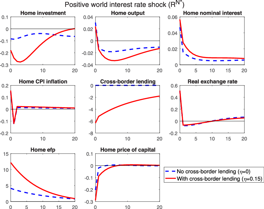
Figure 3 presents the impulse response functions of selected macroeconomic variables in the emerging economy to a one standard deviation rise in the policy rate in the center economy. All variables except the external finance premium are expressed as a percentage of their steady-state values. The external finance premium is expressed as an annualized percentage point deviation from the steady state.
Impulse responses to a one standard deviation rise in the interest rate in center. Blue dashed lines correspond to a calibration without cross-border lending
 $\eta = 0$
. Red solid lines correspond to the baseline calibration, where the share of financing from global banks is
 $\eta = 15\%$
. All values except for the responses of the external finance premia are in percentage deviations from the steady state
 $(x_{t}-\bar{x})/\bar{x}\times 100$
. The responses of the external finance premia are presented as annualized percentage point deviations from the steady state.

A rise in the policy rate in the center has an amplification effect due to financial frictions and leads to large fall in investment and real activity. The impulse responses in the center (not shown) is similar to that in BGG (1999) due to the center’s overwhelming size. We are interested in the propagation of the shock to the emerging economy, which comes through three channels. The first is a standard expenditure switching channel present as in models such as Backus et al. (Reference Backus, Kehoe and Kydland1992). The external interest rate shock induces a real exchange rate depreciation in the emerging economy, so demand in both economies switches toward goods produced in the emerging economy. This effect tends to generate a negative international comovements between consumption, investment, and output. A second channel, termed by Faia (Reference Faia2007) as a financial spillover channel, has the opposite effect. When aggregate demand increases, the interest rate in the emerging economy rises to clear the goods market. Monetary tightening reduces demand for capital and its price, thus increasing the external finance premium. This works through the financial accelerator effect in the emerging economy.
The presence of these two channels is not related to cross-border lending by global banks. The blue dashed lines in Figure 3 report what happens when
 $\eta =0$
(i.e. when entrepreneurs in the emerging economy do not borrow from global banks). It shows a rise in the nominal interest rate and the external finance premium. As a result, the increase in output (coming from the expenditure switching channel) is short-lived, and investment falls from the very beginning.
When entrepreneurs borrow from global banks, a third, cross-border lending channel comes into play. The red solid lines show the impulse responses when a share of
 $\eta=0.15$
of entrepreneurial borrowing comes from global banks. The cross-border lending channel is as follows: an unexpected tightening of monetary policy in the center reduces the return on capital and so the return to global banks and their net worth, and thereby increases their default probability. Because global banks lend to entrepreneurs in both the center and the emerging economy, the external finance premium rises in both countries. Cross-border lending to the emerging economy falls substantially. At the same time, a rise in the external finance premium also reduces the price of capital, which affects local banks through a financial accelerator mechanism in the emerging economy. A comparison with the blue dashed lines (without cross-border lending) reveals the importance of the common-lender effect of financial integration. The global banking network leads to stronger and more volatile spillovers of monetary shocks to the emerging economy, almost doubling the fall in output and tripling the fall in investment. The response in the external finance premium is about 2–3 times more volatile and the fall in the price of capital is also amplified.
5.2. Financial Risk Shocks
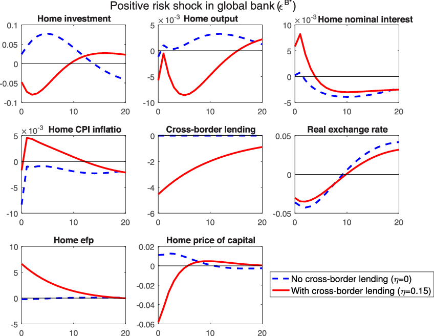
An advantage of this framework is the way financial risk shocks are embedded naturally as a disturbance to the dispersion of the return to global banks’ capital. Figure 4 illustrates the dynamic response of selected variables in the emerging economy to a one standard deviation rise in cross-sectional volatility in global bank risk,
 $s_{t}^{B*}$
. As before, red solid lines (blue dashed lines) display the impulse responses with (without) cross-border lending.
Impulse responses to a one standard deviation rise in global bank risk. Blue dashed lines correspond to a calibration without cross-border lending
 $\eta = 0$
. Red solid lines correspond to the baseline calibration, where the share of financing from global banks is
 $\eta = 15\%$
. All values except for the responses of the external finance premia are in percentage deviations from the steady state
 $(x_{t}-\bar{x})/\bar{x}\times 100$
. The responses of the external finance premia are presented as annualized percentage point deviations from the steady state.

Recall that financial risk increases the dispersion of the distribution of idiosyncratic shocks. More global banks go bankrupt, and
 $\rho^{B*}(\tilde{\omega}^{B*})$
rises, which disrupts the supply of credit in the center. As a result, production falls and demand shifts to the emerging economy. When there is no cross-border lending, which corresponds to the blue dashed lines in Figure 4, this demand shifting effect leads to a rise in investment in the emerging market, a modest rise in asset prices and a fall in the external finance premium. However, the negative business cycle comovement is inconsistent with key stylized facts of the global financial cycle.
When the emerging market borrows
 $\eta = 15\%$
of their funds from global banks (red lines), the investment dynamics are reversed. This effect is driven by a co-movement of the external finance premia in the center and the emerging economy, as shown in the first-order conditions (9) and (10)1. For the emerging economy, a rise in the external finance premium means that the required return on capital rises and the price of capital
 $Q_{t}$
falls. This triggers an amplification due to financial market imperfection which reduces local banks’ ability to intermediate funds as well. With global financial linkages, the emerging economy is more exposed to external financial risks, with a much deeper and more persistent fall in output. Note also that cross-border lending to the emerging economy drops persistently when financial risk rises in the center, driven by global banks’ financial linkages.
6 Monetary and Capital Account Policies
The emerging market above uses an ad hoc monetary policy rule which is suboptimal. This section further investigates the policy options of the emerging economy in response to financial shocks in the center. I study the welfare effects of different monetary and capital account policies.
Following Farhi and Werning (Reference Farhi and Werning2014), capital control is modeled as a tax or subsidy on capital flows in the emerging economy. Denote
 $\tau_{t}$
as a tax/subsidy such that:
 \begin{eqnarray}R^{B*}_{t} X^{*}_{t-1} &=& (1-\tau_{t})\frac{m}{1-m} \eta \frac{\left[\Gamma^{E\times}\left(\tilde{\omega}^{E\times}_{t}\right) - \mu^{E\times} G^{E\times}\left(\tilde{\omega}^{E\times}_{t}\right)\right] R^{E}_{t} Q_{t-1} K_{Ft-1}}{S_{t}} \nonumber \\&&+ \left[\Gamma^{E*}\left(\tilde{\omega}^{E*}_{t}\right) - \mu^{E*}G^{E*}\left(\tilde{\omega}^{E*}_{t}\right) \right] R^{E*}_{t}Q^{*}_{t-1}K^{*}_{t-1}. \end{eqnarray}
The proceeds of the tax are rebated lump-sum to the households in the emerging economy. The tax is assumed to follow a simple rule, given by:
 \begin{equation}\tau_{t} = \Upsilon \left( \frac{\Xi_{t}}{\bar{\Xi}} - 1\right), \qquad \Upsilon \geq 0, \end{equation}
where
 $\Xi_{t} = \frac{m}{(1-m)}\eta\frac{(Q_{t}K_{Ft}-N^{E}_{t})}{S_{t}}$
is the size of cross-border capital flow to the emerging economy. The parameter
 $\Upsilon$
is nonnegative so when cross-border flow is above (below) equilibrium, the emerging economy imposes a tax (subsidy) on the flow. The magnitude of the parameter
 $\Upsilon$
governs the sensitivity of capital controls to the size of cross-border flows.
In the presence of a tax on cross-border capital flow, global banks’ first-order condition for cross-border lending, (10), has an additional tax term:
 \begin{equation}E_{t}\left( \frac{R_{t+1}^{E}}{R_{t}} \right) = E_{t} \left[ \rho^{B*}\left(\tilde{\omega}_{t+1}^{B*}; s_{t}^{B*}\right) \times \rho^{E\times}\left(\tilde{\omega}_{t+1}^{E\times}; s_{t}^{E\times}\right) \times \frac{1}{(1-\tau_{t+1})} \right]\!, \quad \text{for} \;\; \eta >0. \end{equation}
A positive
 $\tau_{t}$
reduces the average gross revenue of global banks, so they require a higher expected return to capital for the entrepreneurs in the emerging economy.
In the following, I study (i) a fixed exchange rate regime, (ii) a flexible exchange rate regime with an optimal simple rule, and (iii) a flexible exchange rate regime with capital controls.
Footnote 14
In the fixed exchange rate regime, the coefficients of the monetary policy rule is set to
 $\phi_{\mathscr{E}}=999$
and
 $\phi_{\pi}=\phi_{Y}=0$
, which ensures that the nominal interest rate in the two economies is equalized. In the flexible exchange rate regime with an optimal simple rule, I set
 $\phi_{\mathscr{E}}=0$
and choose coefficients using a grid search in
 $\phi_{\pi}, \phi_{Y} \in [1.001,10] \times [0,0.5]$
to maximise household utility (15)1. When capital controls are available, the sensitivity of tax on global bank capital outflows is set to
 $\Upsilon = 0.005$
, and monetary policy coefficients
 $\{\phi_{\pi}, \phi_{Y}\}$
are chosen optimally using a grid search.
Footnote 15
To compare welfare across different regimes, I define
 $\xi_{k}$
as the percentage change of deterministic steady-state consumption that gives the same expected utility under policy regime k for a given shock. Following Schmitt-Grohe and Uribe (Reference Schmitt-Grohe and Uribe2007), the welfare measurement used here is the unconditional expected lifetime utility of the representative household (15). The value of
 $\xi_{k}$
for regime k is given by:
 \begin{equation}\frac{1}{1-\beta} u( \bar{C}(1+\xi_{k}), \bar{L}_{C}) = U_{k},\end{equation}
where
 $U_{k}$
is the expected lifetime utility under policy regime k. The system is solved numerically using the second-order approximation around the non-stochastic steady state.
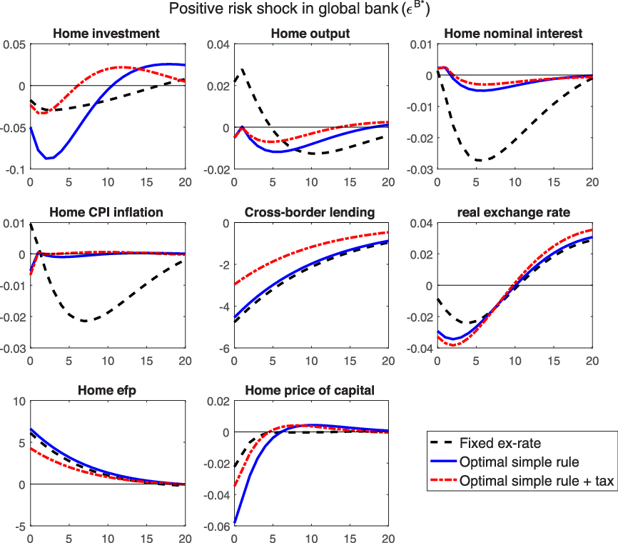
Figure 5 shows the adjustment paths in response to a rise in financial risk in the global banking sector. A fixed exchange rate regime (black dashed line) is not helpful in absorbing the spillover effect of this external shock. The shock induces a monetary policy easing in the center, and the emerging economy cuts the policy rate strongly to maintain the peg, which leads to a relatively smooth real exchange rate path. Although an immediate fall in output is prevented and investment falls by less, the dynamic adjustment paths of output and inflation are more volatile and persistent. Monetary easing also makes cross-border bank lending unattractive, reducing its size. The fact that a fixed exchange rate regime generates too much volatility in the real economy and is suboptimal is well understood from the traditional open economy models such as Gali and Monacelli (Reference Gali and Monacelli2005).
Impulse responses to a one standard deviation rise in global bank risk. Under a fixed exchange rate regime,
 $\{\phi_{\pi}, \phi_{Y}, \phi_{\mathscr{E}} \} = \{0, 0, 999\}$
. Under the optimal simple rule without capital controls,
 $\{\phi_{\pi}, \phi_{Y}, \phi_{\mathscr{E}} \} = \{1.62, 0.219, 0\}$
. Under the optimal simple rule with capital controls,
 $\{\phi_{\pi}, \phi_{Y}, \phi_{\mathscr{E}} \} = \{1.95, 0.223, 0\}$
. All values except for the responses of the external finance premia are in percentage deviations from the steady state
 $(x_{t}-\bar{x})/\bar{x}\times 100$
. The responses of the external finance premia are presented as annualized percentage point deviations from the steady state.

Under the optimal monetary policy (blue solid line), the emerging market chooses
 $\phi_{\pi}=1.62$
and
 $\phi_{Y}=0.22$
. The nominal interest rate falls by much less, keeping CPI inflation stable and output less volatile. On the other hand, because monetary policy is less accommodative, the initial fall in investment and the price of capital (amplified by BGG frictions) is large. Comparing the responses of the two exchange rate regimes, it is evident that monetary policy carries the burden of maintaining macroeconomic and financial stability.
Footnote 16
Finally, under either exchange rate regime, there is a sizable fall in global bank lending to the emerging economy.
The red dash-dotted lines show what happens when capital controls are used alongside an the optimal simple monetary rule. Following a rise in global bank risk, the tax rate
 $\tau_{t}$
becomes negative, which means that the emerging economy provides a subsidy to cross-border bank lending. The first-order condition of global bank (33) shows that this capital account policy effectively limits capital outflows and the increase in the external finance premium, which moderates the amplification effect of the financial accelerator. As the capital control policy partly takes care of financial stability, the nominal interest rate need not fall as much to bolster investment and focuses on maintaining macroeconomic stability. To see this, note that the inflation feedback coefficient in the monetary policy rule,
 $\phi_{\pi}$
, increases from
 $1.62$
to
 $1.95$
(while
 $\phi_{Y}$
is almost unchanged) when the emerging market has capital controls policy.
Footnote 17
6.1 Sensitivity Analysis
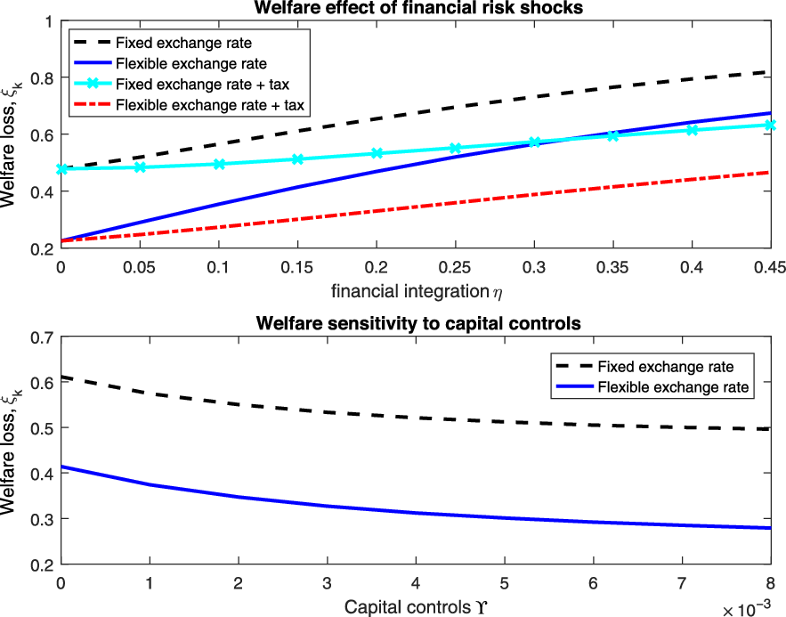
Figure 6 shows the welfare losses in the emerging economy generated by financial risk shocks under different monetary policy regimes. The top panel shows what happens when the degree of financial integration
 $\eta$
is varied. Under a fixed exchange rate, the policy rate of the emerging economy follows the center. In a flexible exchange rate regime, I assume that the Taylor rule is based on the optimized parameter (
 $\phi_{\pi}=1.62$
and
 $\phi_{Y}=0.22$
). Under each of the two exchange rate regimes, I also study a specification which allows the emerging market to tax/subsidize global bank outflows according to the capital control rule (32) with
 $\Upsilon$
fixed at
 $0.005$
.
Welfare loss in the emerging economy (in percentage units of steady-state consumption). The top panel shows welfare loss with various degree of financial integration. The bottom panel shows welfare loss with various sensitivities of capital controls to cross-border flows
 $\Upsilon$
, when financial integration is fixed at
 $\eta =0.15$
. Under a fixed exchange rate regime,
 $\{\phi_{\pi}, \phi_{Y}, \phi_{\mathscr{E}} \} = \{0, 0, 999\}$
. Under the flexible exchange rate regime,
 $\{\phi_{\pi}, \phi_{Y}, \phi_{\mathscr{E}}\}=\{1.62,0.22,0\}$
. In the top panel, when tax or subsidy is available, the degree of capital controls is set to
 $\Upsilon=0.005$
.

As
 $\eta$
increases from 0 to
 $0.4$
, although the flexible exchange rate regime always fares better than a peg, the welfare loss triples (from
 $0.0022$
to
 $0.0067$
). This is because cross-border lending is an additional channel through which shocks from the center affect the emerging economy, and monetary policy cannot smooth the business cycle and capital flows at the same time. In this way, financial integration weakens the stabilization effect of independent monetary policy. Indeed, as Rey (Reference Rey2018) and Obstfeld (Reference Obstfeld, Raddatz, Saravia and Ventura2015) point out, a larger degree of financial integration reduces the welfare gap between flexible and fixed exchange rate regimes.
Temporary capital controls improve welfare in a flexible exchange rate regime. This agrees with the observation that capital controls smooth fluctuations in the impulse response functions. Moreover, capital controls improve welfare in a fixed exchange rate regime as well. This policy works from the bank lending channel in (33) and is independent of the choice of exchange rate regime. The extent to which temporary capital controls improve welfare depends crucially on the financial integration of the emerging economy. The more financially integrated the economy is, the more useful the capital controls are. When the emerging market is sufficiently open (above
 $0.3$
), capital account policies appear to be more useful than monetary policy.
The bottom panel of Figure 6 displays how much welfare improves when capital controls with different sensitivities to cross-border lending
 $\Upsilon$
are implemented, while financial openness is fixed at
 $\eta=0.15$
. Two results emerge. First, for either regime, welfare loss is monotonically decreasing in the sensitivity of capital controls. The reason for this is similar to Aoki et al. (Reference Aoki, Benigno and Kiytoaki2016). Capital controls, modeled in this way, only impact the bank lending channel, and have no direct effect on households’ consumption smoothing decision, so welfare is always increasing with the capital control parameter
 $\Upsilon$
.
Footnote 18
As discussed above, this channel operates independently of the exchange rate regime, so the welfare gap between two regimes is almost constant. Second, capital controls need not be very sensitive to cross-border flows. When the sensitivity parameter
 $\Upsilon$
is large (say, above 0.005), the marginal welfare improvement is limited.
7 Conclusions
This paper analyses a core–periphery model with cross-border bank lending to shed light on the international transmission of financial risks to emerging economies through the global banking network. The key analytical insight is that lenders to global banks indirectly lend to borrowers in both the center and emerging economy, and so a rise in financial risk results in a synchronized increase in external financial premia.
I consider monetary and capital account policies in an emerging economy facing external financial risks. Spillovers increase with financial integration, worsening the trade-off between maintaining macroeconomic stability and continuous capital inflows. This paper shows that, under financial integration, although a flexible exchange rate regime with an appropriate monetary policy fares better than a fixed exchange rate regime and the trilemma remains true, the welfare gap between a peg and a flexible exchange rate regime shrinks. I show that capital controls in the form a temporary tax or subsidy to bank capital flows can moderate the trade-off between macroeconomic stability and capital flow stability, which is welfare-enhancing.
ACKNOWLEDGMENTS
I would like to thank Feng Dong, Xu Hu, Sang Seok Lee, Ka Fai Li, Byron Kwok Ping Tsang, Kozo Ueda, David Vines, Tommy Wu, Zhiwei Xu, Tianxiao Zheng, and conference and seminar participants at 2017 Asian Meeting of the Econometric Society, 3rd HenU/INFER Workshop on Applied Macroeconomics, Hong Kong Shue Yan University, Shanghai Jiaotong University, and Shanghai University of International Business and Economics for their helpful comments. Financial support from Hong Kong Research Grants Council Early Career Scheme (Project No. 22500716) is gratefully acknowledged. This paper represents the views of the author, which are not necessarily the views of the Hong Kong Monetary Authority, the Hong Kong Institute for Monetary, and Financial Research or its Board of Directors.
Appendix A: Empirical Evidence
This section provides empirical evidences of the financial risk channel of international spillover. I first construct data for financial risk and cross-border claims to emerging market economies. I use the Chicago Board Options Exchange VIX index to proxy financial risk. The cross-border claims series for the period 1990Q1–2018Q1 is constructed from Bank for International Settlements locational banking statistics. I compute the total foreign claims by US banks to counterparty countries which belong to an emerging economy. Out of all reporting countries, I remove all countries with missing observations during the sample period, G7 economies, Eurozone economies, and offshore financial centers (defined by the International Monetary Fund. See https://www.imf.org/external/np/mae/oshore/2000/eng/back.htm). I remove G7 economies because the focus on this paper is emerging economies. Eurozone global banks are removed because they are heavily involved in drawing wholesale funding from the USA and then lending it back to US residents, as shown in Shin (Reference Shin2012). Offshore financial centers are removed because they mainly channel financial transactions in the rest of the world and are unlikely to be the final destination of cross-border bank lending. This leaves me with 34 economies including: Argentina, Australia, Brazil, Chile, China, Chinese Taipei, Colombia, Denmark, Ecuador, Egypt, Guatemala, Hungary, India, Indonesia, Israel, Jamaica, Lebanon, Liberia, Malaysia, Mexico, Morocco, Norway, Pakistan, Peru, Philippines, Poland, South Africa, South Korea, Sweden, Thailand, Trinidad and Tobago, Turkey, Uruguay, and Venezuela.
Figure 1 presents the linearly detrended cross-border claims series together with the log of the VIX index. The negative correlation is robust to using the log-difference of cross-border lending.
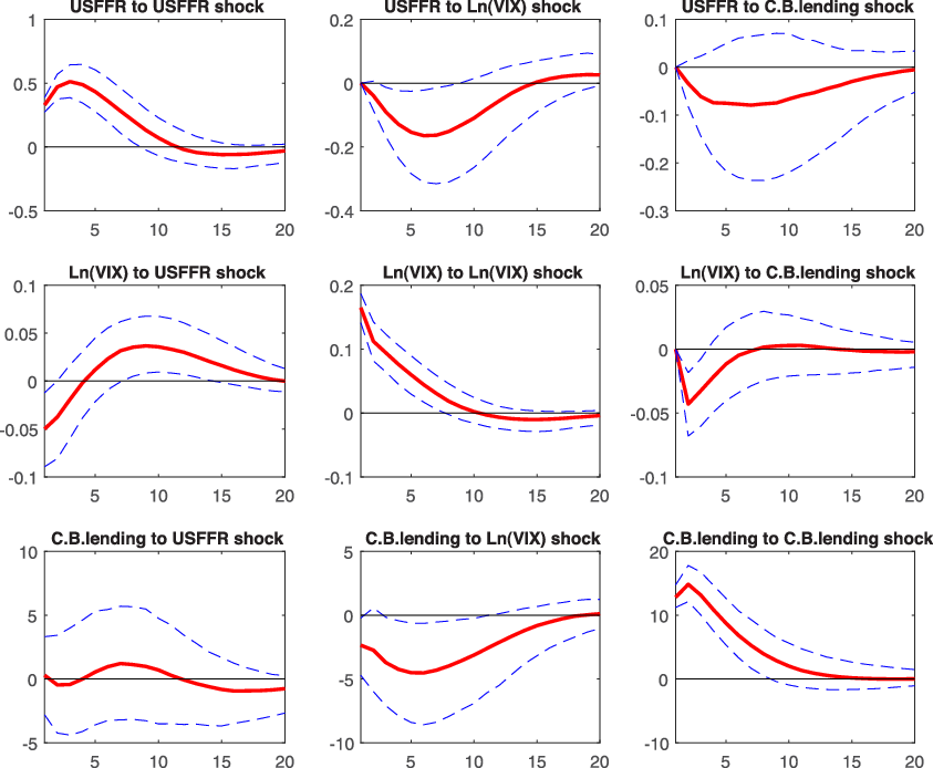
Next, I use a recursive vector autoregressive (VAR) model examining the dynamic relationship between US monetary policy, financial risk, and cross-border lending to emerging markets. The sample consists of quarterly data of US monetary policy (the nominal effective federal funds rate), the VIX index and US cross-border lending to emerging market during the period 1990Q1–2018Q1.
The structural VAR model follows Bekaert et al. (Reference Bekaert, Hoerova and Duca2013), Bruno and Shin (Reference Bruno and Shin2015), and Rey (Reference Rey2018). The key difference between the present model and the existing literature is that I focus on claims to emerging economies, whereas the rest of the literature considers total financial flows (which is dominated by financial transactions between USA and Europe). The identification scheme imposes Cholesky restrictions, so that variables ordered in front do not respond to contemporaneous shocks behind. The Federal Funds rate (USFFR) is placed first, because it is determined based a periodic decision process. The VIX index is ordered second to capture unanticipated financial risk shocks orthogonal to US monetary policy surprises. The cross-border claims (CBlending) are the last. Note that this ordering is consistent with the structural model to be presented, in which I study the impacts of the same structural (monetary policy and financial risk) shocks from the USA. The VAR is specified with two lags, using Bayesian information criteria and likelihood ratio as the lag selection criteria.
Figure A1 presents the impulse response functions, with 86% bootstrapped confidence intervals computed using 1000 replications. The key finding is that a positive shock to the VIX index leads to a persistent fall in cross-border lending to emerging economies, for about 10 quarters. The sizable and long-lasting fall in cross-border lending echoes a key empirical finding in Bruno and Shin (Reference Bruno and Shin2015) that shocks in the USA (in particular, the broker–dealer leverage) have a marked influence on cross-border flows. But here, I only focus on the effect on emerging economies. The shock also leads to a decline in the US federal funds rate for about 2 years. It is also noted that the response of VIX to a rise in the federal funds rate is qualitatively similar to Bekaert et al. (Reference Bekaert, Hoerova and Duca2013) and Rey (Reference Rey2018). The second figure from the first column shows an immediate fall in VIX, followed by an increase in the VIX after about 2 years. Footnote 19
Impulse response functions in recursive VAR. This figure presents estimated impulse response functions for the three-variable VAR (USFFR, VIX, and CBlending), and 86% bootstrapped confidence intervals for the model with two lags, based on 1000 replications.

Overall, the empirical results suggest that financial risk in the USA affects cross-border bank lending from the USA to emerging market economies.
Appendix B: Proof of Proposition 1
I derive the optimal chained credit contract in the global banks. A global bank maximizes the objective:
 \begin{equation*} E_{t} \left[ (1-\Gamma^{B*}(\tilde{\omega}^{B*})) R^{B*} X^{*}\right],\end{equation*}
subject to participation constraints of entrepreneurs (6) and (7) and the participation constraint of the investors in the center (8). The Lagrangian is
 \begin{eqnarray} Lagr. &=& (1-\Gamma^{B*}) R^{B*}X^{*} \nonumber \\ && + \lambda^{*}_{1} \left[ \Psi^{B*} R^{B*}X^{*} - R^{*}\left( \frac{m}{1-m} \eta \frac{QK_{F}-N^{E}}{S}+ Q^{*}K^{*}-N^{E*} -N^{B*}\right) \right] \nonumber \\ && + \lambda^{*}_{2} (QK_{F}(1-\Gamma^{E\times}) - N^{E}) + \lambda^{*}_{3} (Q^{*}K^{*}(1-\Gamma^{E*}) - N^{E*}),\end{eqnarray}
where
 $\lambda^{*}_{1}$
is the Lagrange multiplier to the investors’ participation constraint, and
 $\lambda^{*}_{2}$
and
 $\lambda^{*}_{3}$
are the Lagrange multipliers to participation constraints of entrepreneurs in the emerging economy and the center, respectively, and
 $\Psi^{i} \equiv (\Gamma^{i} - \mu^{i} G^{i})$
.
 $R^{B*}X^{*}$
is given by (31) which is repeated here:
 \begin{equation*} R^{B*} X^{*}= (1-\tau) \frac{m}{1-m}\eta \Psi^{E\times} \frac{R^{E} QK_{F} }{S_{+1}} + \Psi^{E*} R^{E*} Q^{*} K^{*}.\end{equation*}
The first-order conditions are
 \begin{eqnarray}K_{F}&:& \; 0= (1-\Gamma^{B*}) (1-\tau) \frac{m}{1-m}\eta \Psi^{E\times} \frac{R^{E} Q }{S_{+1}} \nonumber \\ && \;\;\; + \lambda_{1}^{*} \left[ \Psi^{B*} (1-\tau) \frac{m}{1-m}\eta \Psi^{E\times} \frac{R^{E} Q }{S_{+1}} - R^{*} \frac{m}{1-m} \eta \frac{Q }{S} \right] + \lambda_{2}^{*} Q (1-\Gamma^{E\times}), \end{eqnarray}
 \begin{eqnarray}K^{*}&:& \; 0= (1-\Gamma^{B*}) \Psi^{E*} R^{E*} Q^{*} \nonumber \\ && \;\;\; + \lambda^{*}_{1} \left[ \Psi^{B*} \Psi^{E*} R^{E*} Q^{*} - R^{*} Q^{*}\right] + \lambda^{*}_{3} Q^{*} (1-\Gamma^{E*}), \end{eqnarray}
 \begin{eqnarray}\tilde{\omega}^{B*}&:& \; 0= - \Gamma^{B*}_{\omega} + \lambda_{1}^{*} \Psi^{B*}_{\omega}, \end{eqnarray}
 \begin{eqnarray}\tilde{\omega}^{E\times}&:& \; 0 = (1-\Gamma^{B*}) (1-\tau)\frac{m}{1-m}\eta \Psi^{E\times}_{\omega} \frac{R^{E} }{S_{+1}}+ \lambda^{*}_{1} \Psi^{B*} (1-\tau) \frac{m}{1-m}\eta \Psi^{E\times}_{\omega} \frac{R^{E} }{S_{+1}}- \lambda^{*}_{2} \Gamma^{E\times}_{\omega}, \nonumber\\ \end{eqnarray}
 \begin{eqnarray}\tilde{\omega}^{E*}&:& \; 0 = (1-\Gamma^{B*}) \Psi^{E*}_{\omega} R^{E*} + \lambda^{*}_{1} \Psi^{B*} \Psi^{E*}_{\omega} R^{E*}- \lambda^{*}_{3} \Gamma^{E*}_{\omega}.\end{eqnarray}
The Lagrange multipliers are
 \begin{eqnarray*} \lambda_{1}^{*} &=& \frac{ \Gamma^{B*}_{\omega} }{\Psi_{\omega}^{B*} }, \\ \lambda^{*}_{2} &=& (1-\tau) \frac{m}{1-m}\eta \frac{ \Psi^{E\times}_{\omega}}{\Gamma^{E\times}_{\omega}} \frac{R^{E} }{S_{+1}} \left[ (1-\Gamma^{B*}) + \frac{\Gamma^{B*}_{\omega}}{\Psi^{B*}_{\omega}} \Psi^{B*} \right], \\ \lambda^{*}_{3} &=& \frac{ \Psi^{E*}_{\omega}}{\Gamma^{E*}_{\omega}} R^{E*} \left[ (1-\Gamma^{B*}) + \frac{\Gamma^{B*}_{\omega}}{\Psi^{B*}_{\omega}} \Psi^{B*} \right].\end{eqnarray*}
Substituting these into the first-order conditions for
 $K_{F}$
and
 $K^{*}$
, rearranging, and simplifying, one obtains
 \begin{eqnarray} 0 &=& \frac{\Gamma^{B*}_{\omega} }{\Psi^{B*}_{\omega} } \left( \frac{(1-\tau)R^{E}}{\rho^{B*} \rho^{E\times} } - \frac{S_{+1}}{S } R^{*} \right), \end{eqnarray}
 \begin{eqnarray} 0 &=& \frac{\Gamma^{B*}_{\omega} }{\Psi^{B*}_{\omega}} \left( \frac{R^{E*}}{\rho^{B*} \rho^{E*} } - R^{*} \right).\end{eqnarray}
where for
 $i \in \{B, B^{*}, E, E^{*}, E^{\times}\}$
:
 \begin{equation}\rho^{i} \equiv \frac{[\Gamma_{\omega}^{i}/(\Gamma^{i}_{\omega} - \mu^{i} G^{i}_{\omega})]}{(1-\Gamma^{i}) + (\Gamma^{i} - \mu^{i} G^{i})[\Gamma_{\omega}^{i}/(\Gamma^{i}_{\omega} - \mu^{i} G^{i}_{\omega})]}.\end{equation}
To derive the properties of the
 $\rho^{i}$
function, we use the property that
 $\log(\omega^{i}) \sim N(-0.5 (s^{i})^{2}, (s^{i})^{2})$
. It is easy to show that for
 $i \in \{B, B^{*}, E, E^{*}, E^{\times}\}$
, the derivatives
 $F_{\omega }^{i}(\tilde{\omega}^{i}), G_{\omega }^{i}(\tilde{\omega}^{i}), \Gamma_{\omega}^{i}(\tilde{\omega}^{i})$
are positive. Furthermore, the first derivatives with respect to
 $s^{i}$
are given by
 $F^{i}_{s} >0, G^{i}_{s} >0, \Gamma^{i}_{s} < 0$
. Finally, with straightforward but tedious arithmetics, one can show the following properties for the second derivatives:
 $G^{i}_{\omega\omega} >0, G^{i}_{\omega s} >0, \Gamma^{i}_{\omega\omega} <0, \Gamma^{i}_{\omega s} <0$
. Using these properties, it is shown that
 $\rho^{i} \geq 1$
, and
 \begin{eqnarray*}\rho^{i}_{\omega} &=& \frac{\mu^{i} (1-\Gamma^{i}) }{[(1-\Gamma^{i})(\Gamma^{i}_{\omega}-\mu^{i} G^{i}_{\omega}) + (\Gamma^{i}-\mu^{i} G^{i}) \Gamma^{i}_{\omega}]^2} ( \Gamma^{i}_{\omega} G^{i}_{\omega\omega}-\Gamma^{i}_{\omega\omega} G^{i}_{\omega} ) > 0. \\\rho^{i}_{s} &=& \frac{ (1-\Gamma^{i})\mu^{i} [ \Gamma^{i}_{\omega} G^{i}_{\omega s} - G^{i}_{\omega}\Gamma^{i}_{\omega s}] + \mu^{i}\Gamma^{i}_{\omega}[\Gamma^{i}_{\omega} G^{i}_{s}-\Gamma^{i}_{s} G^{i}_{\omega}] }{[(1-\Gamma^{i})(\Gamma^{i}_{\omega}-\mu^{i} G^{i}_{\omega}) + (\Gamma^{i} -\mu^{i} G^{i} ) \Gamma^{i}_{\omega}]^2} >0.\end{eqnarray*}
Appendix C: LOCAL BANKS
Banks in the emerging economy intermediate funds by borrowing from local investors and lending to local entrepreneurs. Loans to local entrepreneurs,
 $X_{t}$
, are given by:
 \begin{eqnarray} X_{t} &\equiv& (1-\eta) (Q_{t}K_{Ht}-N^{E}_{t}).\end{eqnarray}
The banks only lend to local entrepreneurs using E contracts. The gross revenue of the banks’ lending is denoted as
 $R^{B}_{t}X_{t-1}$
, and is given by:
 \begin{eqnarray} R^{B}_{t}X_{t-1} &=& (1-\eta) \Psi^{E}(\tilde{\omega}^{E}_{t}) R^{E}_{t}Q_{t-1}K_{Ht-1}.\end{eqnarray}
Gross revenue of the banks is the lender’s share of revenue in the E contract,
 $\Psi^{E}(\tilde{\omega}^{E}_{t})$
, times the total revenue earned by entrepreneurs
 $(1-\eta) R^{E}_{t}Q_{t-1}K_{Ht-1}$
.
Banks have to satisfy the participation constraint of the entrepreneurs in each period
 $t+1$
state of nature:
 \begin{eqnarray} (1-\eta) R^{E}_{t+1}N^{E}_{t} &=& (1-\eta) R^{E}_{t+1}Q_{t}K_{Ht} (1-\Gamma^{E} (\tilde{\omega}^{E}_{t+1})). \end{eqnarray}
This constraint requires that the revenue retained by entrepreneurs (a share
 $(1-\Gamma^{E} (\tilde{\omega}^{E}_{t+1})) $
of the total revenue) has to be greater than the revenue from operating solely with their own funds. Moreover, they have to satisfy the participation constraint of investors in each period
 $t+1$
state of nature, given by:
 \begin{eqnarray} R_{t}(X_{t} -N^{B}_{t}) &=& \Psi^{B}(\tilde{\omega}_{t+1}^{B}) R^{B}_{t+1} X_{t}. \end{eqnarray}
This constraint requires that the fraction of bank revenue that goes to investors, after deducting monitoring costs, has to be as big as the risk-free return.
Banks in the emerging economy maximize their expected profit:
 \begin{eqnarray*} E_{t} \{ [1-\Gamma^{B}(\tilde{\omega}^{B}_{t+1})] R^{B}_{t+1} X_{t}\}, \nonumber\end{eqnarray*}
by choosing
 $\{K_{Ht}, \tilde{\omega}^{B}_{t+1}, \tilde{\omega}^{E}_{t+1}\}$
, subject to participation constraints (C3) and (C4). The symbol
 $E_{t}$
is the mathematical expectation. The
 $(\tilde{\omega}^{B}_{t+1}, \tilde{\omega}^{E}_{t+1}, K_{Ht})$
combinations which satisfy (C3) and (C4) define a menu of state
 $(t+1)$
-contingent chained credit contracts available to the local banks.
Following similar derivation as in the optimal contract for global banks (details shown in Appendix B), the first-order condition for banks in the emerging economy is given by:
 \begin{eqnarray} 0 &=& E_{t} \left[ \frac{1}{\rho^{B}(\tilde{\omega}^{B}_{t+1}) \rho^{E}(\tilde{\omega}^{E}_{t+1})} - \frac{R_{t}}{R^{E}_{t+1}} \right] . \end{eqnarray}
Appendix D: CALIBRATION OF THE FINANCIAL CONTRACTS
I discuss the calibration of the financial contracts. I use the following steady-state conditions:
 \begin{eqnarray} \frac{\bar{R}^{E}}{\bar{R}} &=& \rho^{B}(\bar{\tilde{\omega}}^{B};\bar{s}^{B}) \times \rho^{E}(\bar{\tilde{\omega}}^{E}; \bar{s}^{E}), \end{eqnarray}
 \begin{eqnarray} \frac{\bar{N}^{E}}{\bar{K}} &=& 1- \Gamma^{E}(\bar{\tilde{\omega}}^{E}; \bar{s}^{E}), \end{eqnarray}
 \begin{eqnarray} \frac{\bar{R}^{E}}{\bar{R}} \times \Psi^{B}(\bar{\tilde{\omega}}^{B}; \bar{s}^{B}) \times \Psi^{E}(\bar{\tilde{\omega}}^{E}; \bar{s}^{E}) &=& 1- \frac{\bar{N}^{E}}{\bar{K}} -\frac{\bar{N}^{B}}{\bar{K}},\end{eqnarray}
where the first equation is the first-order condition for bank’s optimal contract, the second is the participation constraint of the entrepreneurs, and the third is the participation constraint of the investors in economy without financial integration.
The accumulation of bank net worth implies
 \begin{equation} \frac{\bar{N}^{E}}{\bar{K}} \frac{\bar{K}}{\bar{Y}} = \gamma^{B} [1-\Gamma^{B}(\bar{\tilde{\omega}}^{B};\bar{s}^{B})] \Psi^{E}(\bar{\tilde{\omega}}^{E}; \bar{s}^{E}) \bar{R}^{E}\frac{\bar{K}}{\bar{Y}} + \Omega^{B}(1-\alpha),\end{equation}
where the steady-state capital to output ratio is given by
 $\bar{Y}/\bar{K} =\alpha^{-1}[\bar{R}^{E} -(1-\delta)]$
.
Furthermore, the ratio of contractual interest rates is
 \begin{eqnarray} \frac{\bar{Z}^{E}}{\bar{Z}^{B}} = \frac{\bar{\tilde{\omega}}^{B}\Psi^{E}(\bar{\tilde{\omega}}^{E}; \bar{s}^{E}) \left(1-\frac{\bar{N}^{E}}{\bar{K}}\right)}{\bar{\tilde{\omega}}^{E}\left(1- \frac{\bar{N}^{E}}{\bar{K}} -\frac{\bar{N}^{B}}{\bar{K}} \right)}.\end{eqnarray}
Given the bank and firm default probabilities, we have seven equations to solve for
 $\{\bar{\tilde{\omega}}^{B}, \bar{\tilde{\omega}}^{E}\}$
and the five parameters
 $\{ \mu^{E}, \mu^{B}, \bar{s}^{E}, \bar{s}^{B}, \gamma^{B} \}$
. The survival rate of entrepreneurs
 $\gamma^{E}$
can be backed out using the steady-state evolution equation of entrepreneurs’ net worth.