1.1 Preliminaries

Many people have an intuitive understanding of probability as either the long run limit of a series of random experiments, or a subjective belief of what is likely to happen in a given situation. To introduce this topic in a more rigorous manner, a short background will be given here, in order to introduce terminology and notation. To start with, a sample space Ω is defined as a set of outcomes, that is, Ω = {ω ₁, ω ₂, … , ω_n}. An event E on Ω is a subset of Ω, that is, E ⊆ Ω. From this point of view, outcomes may be seen as elementary events, that is, events that can only take on a true/false character. Events are things which we might be interested in and tend to be the fundamental unit of probability theory. A probability distribution P, is a function from the space of events to the space of real numbers from 0 to 1, that is, , where is the power set of Ω. So when we say the probability of an event E is 0.76, we are saying P(E) = 0.76. Since events are sets, we can perform set operations on them. This allows us to specify the probability of two events, E and F occurring, by P(E ∩ F). From this we can define another very useful idea, that of conditional probability.

The conditional probability of an event E occurring, given that an event F has occurred is given by

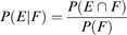
Obviously for this to be defined, P(F) must be strictly positive. As an aside, it should be noted that

This implies that

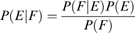
This is the well-known Bayes’ formula and is in itself fundamental to many modern statistical techniques in machine learning. The term P(E|F) is often known as the posterior probability of E given F. The term P(F|E) is often referred to as the likelihood of E given F and the term P(E) is the prior or marginal probability of E. The term P(F) is a normalizing term that is often expanded out as

where H is a set of pairwise disjoint events H_i such that H ₁ ∪ H ₂ ∪ … ∪ H_n = Ω. The reason for this expansion is that the terms P(F|H_i) and P(H_i) are often much easier to obtain than P(F).

Given the definition of conditional probability, we can now define what it means for events to be independent. Two events, E and F are independent if

If P(E) and P(F) are both positive, then both equations imply the other. This definition leads to that of conditional independence, which will involve a third event. Two events, E and F are conditionally independent, given another event G if

Again, these are equivalent if P(E), P(F) and P(G) are strictly positive. The notion of conditional independence is central to Bayesian networks and many other models dealing with probabilistic relationships. It is often given its own notation as E _PF|G, which means that event E is conditionally independent of event F given event G, under probability distribution P.

To complete this subsection, the concepts of random variables and joint probability will be explored. In common parlance, random variables are variables that can take on a value from a given set, and have a certain probability associated with taking on this value. Technically, a random variable X is a function from a sample space Ω to a measurable space M. To illustrate how they are used in practice, imagine the following scenario. Say we are dealing with temperature and we have three different measures of it: low, medium and high. We could then state that the random variable X stands for temperature and our measurable space M is the set {low, medium, high}. So when we make the statement P(X = low), the probability that the temperature is low, the expression X = low is an event E. Therefore, we are calculating P(E), such that E = {ω|ω∈Ω, X(ω) = low}. Normally, we leave all the details of sample space and probability measure implicit and never mention them. Instead we deal directly with random variables, but it is beneficial to know where the notation originates from.

Finally, the joint distribution of a set of random variables is the multidimensional analogue of the single variable case. For example, P(X,Y) is the joint distribution of two random variables X and Y. To specify a probability for an event, we assign values to the variables. P(X = x, Y = y) is the probability that X takes on value x and Y takes on value y. We can marginalize across some of the variables by adding up across all possible values of those variables. For example, given P(X,Y) we can get the probability distribution P(X) by

where M(Y) is the domain (or measure space) of Y. It is useful to note that with the notation P(x, y), where x and y are lower case letters, there are usually implied random variables, so that X = x and Y = y, that is, P(x, y) ≡ P(X = x, Y = y).

1.2 Bayesian networks

To see why conditional independence is important, imagine the following scenario. Say we wanted to define a joint probability distribution across many variables P(X ₁, X ₂, … , X_n). If each variable is binary valued, then we need to store 2ⁿ−1 values. It should be obvious that with this storage requirement exponential in the number of variables, things soon become intractable. To get around this, first note the identity

Now, say that X _1P{X ₃, … ,X_n}|X ₂, that is, X ₁ is independent of the rest of the variables given X ₂. Then,

Notice how the expression involving X ₁ has become much shorter and we have a slightly smaller joint term (minus X ₁). If we can find conditional independencies for the rest of the variables such that this factorization can proceed in a chain like fashion, we will be left with a product of terms, each of which will only contain (hopefully) a small number of random variables. Then, to construct the joint, we need to only specify a number of conditional probability distributions. The reasons for doing the factorization this way are twofold. First, if each variable is conditionally independent of most others, then we only need specify a small number of values for each distribution. Second, humans generally find it easier to specify the values of a conditional distribution.

There are many statistical models that take advantage of these properties. Examples can be found in the paper by Lauritzen and Wermuth (Reference Lauritzen and Wermuth1989) and the books by Castillo et al. (Reference Castillo, Gutiérrez and Hadi1997a), Pearl (Reference Pearl1988) and Whittaker (Reference Whittaker1990). The particular model that will be dealt with here is the Bayesian network. Before defining what they are, some definitions relating to graphs will be given.

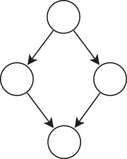
A graph is given as a pair (V, E), where V = {v ₁,…,v_n} is the set of vertices or nodes in the graph and E is the set of edges or arcs between the nodes in V. A directed graph is a graph where all the edges have an associated direction from one node to another. A directed acyclic graph or DAG, is a directed graph without any cycles, that is, it is not possible to return to a node in the graph by following the direction of the arcs. For illustration, the graph in Figure 1 is a DAG. The parents of a node v_i, Pa (v_i), are all the nodes v_j such that there is an arrow from v_j to v_i (v_j → v_i). The descendants of v_i, D (v_i), are all the nodes reachable from v_i by following the arrows repeatedly. The non-descendants of v_i, ND (v_i), are all the nodes that are not descendants of v_i.

Figure 1

A directed acyclic graph

Let there be a graph and a joint probability distribution P over the nodes in V. Say also that the following is true

That is, each node is conditionally independent of its non-descendants, given its parents. Then it is said that satisfies the Markov condition with P, and that is a Bayesian network. Notice the conditional independencies implied by the Markov condition. They allow the joint distribution P to be written as the product of conditional distributions; P (v ₁, v ₂, … , v_n) = P (v ₁|Pa (v ₁))P (v ₂|Pa (v ₂))···P (v_n|Pa (v_n)). However, more importantly, the reverse can also be true. Given a DAG and either discrete conditional distributions or certain types of continuous conditional distributions (e.g. Gaussians), of the form P(v_i|Pa(v_i)) then there exists a joint probability distribution P (v ₁, v ₂, … , v_n) = P (v ₁|Pa (v ₁)) P (v ₂|Pa (v ₂))···P (v_n|Pa (v_n)). This means that if we specify a DAG—known as the structure—and conditional probability distributions for each node given its parents—known as the parameters—we have a Bayesian network, which is a representation of a joint probability distribution.

It may be asked whether there are any other conditional independencies that may be obtained from the Markov condition. It turns out that there are and these can be identified by a property known as d-separation, which is a purely graphical test, that is, a test that can be implemented by performing a search on a graph. The notation means that the nodes in set A are d-separated from the nodes in set B, given set C. It is also the case that given the Markov condition, d-separation is a sufficient condition for conditional independencies in P. That is, for all mutually disjoint subsets A, B and C of V. If a graph can be found such that , then it is said that is faithful to P. Coupled with the Markov condition, this gives and it can be said that is a perfect-map of P. This is important because it implies that the arcs in the graph directly model dependencies between variables, whereas up to now only independencies have been discussed. This brings the structure of the Bayesian network closer to human intuition, in that an arc between two nodes implies there is a direct relation between those variables.

Finally, if it is assumed that in a Bayesian network, an arc from x to y means that x is a direct cause of y, then at least one of a number of causal assumptions is being made, such as the causal Markov assumption or the causal faithfulness assumption. These state that an effect is independent of its non-effects, given its direct causes and that the conditional independencies in the graph are equivalent to those in its probability distribution (see Druzdzel & Simon, Reference Druzdzel and Simon1993; Spirtes et al., Reference Spirtes, Glymour and Scheines2000; Neapolitan, Reference Neapolitan2004; Huang & Valtorta, Reference Huang and Valtorta2006; Valtorta & Huang, Reference Valtorta and Huang2008 for more on these assumptions). If this is the case, then this Bayesian network is capturing knowledge in a succinct way that is immediately obvious to humans, yet also with a well-understood formalism underlying the operations that can be performed. It is for these reasons that Bayesian networks are so popular and a recent book by Kjaerulff and Madsen (Reference Kjaerulff and Madsen2008) shows various ways to capture this type of knowledge in Bayesian network form. As mentioned before, there exist other structures that model conditional independencies, such as Markov fields, that seem to be less popular because of their opaqueness. For a more in-depth look at the differences and similarities of these structures, see the paper of Smyth (Reference Smyth1997). In addition, for a look at the explanatory properties of Bayesian networks see the papers of Druzdzel (Reference Druzdzel1996) and Madigan et al. (Reference Madigan, Mosurski and Almond1997). The relationship between Bayesian networks and causality is sometimes fraught, but there are methods as described in Section 4.8, that mean a causal interpretation can be valid. For more on the intersection of Bayesian networks and causal models see Section 4.2 and the books of Glymour and Cooper (Reference Glymour and Cooper1999), Spirtes et al. (Reference Spirtes, Glymour and Scheines2000) and Pearl (Reference Pearl2000).

1.3 Markov equivalent structures

For the purposes of this article, it is necessary to define some further terms relating to the structures of Bayesian networks. These terms arise because of the redundancies in the DAG representation of the structure, which occur when looking at a Bayesian network as a factorization of a joint probability distribution (as opposed to the causal point of view, where there are no redundancies in the DAG representation).

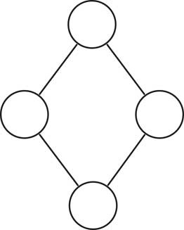
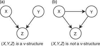
It has been known for some time that there are DAGs that are equivalent to one another, in the sense that they entail the same set of conditional independencies as each other, even though the structures are different. According to a theorem by Verma and Pearl (Reference Verma and Pearl1991), two DAGs are equivalent, if and only if they have the same skeletons and the same v-structures. By skeleton, it is meant that the undirected graph that results from undirecting all edges in a DAG and by v-structure (sometimes referred to as a morality), it is meant a head-to-head meeting of two arcs, where the tails of the arcs are not joined. These concepts are illustrated in Figures 2 and 3. From this notion of equivalence, a class of DAGs that are equivalent to each other can be defined, notated here as .

Figure 2

The skeleton of the DAG in Figure 1

Figure 3

v-structures

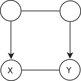
To represent the members of this equivalence class, a different type of structure is used, known as a partially directed acyclic graph (PDAG). A PDAG (an example of which is shown in Figure 4) is a graph that contains both undirected and directed edges and that contains no directed cycles and will be notated herein as . The equivalence class of DAGs corresponding to a PDAG is denoted as , with a DAG , if and only if and have the same skeleton and same set of v-structures.

Figure 4

A partially directed acyclic graph

Related to this is the idea of a consistent extension. If a DAG has the same skeleton and the same set of v-structures as a PDAG , then it is said that is a consistent extension of . Not all PDAGs have a DAG that is a consistent extension of itself. If a consistent extension exists, then it is said that the PDAG admits a consistent extension. Only PDAGs that admit a consistent extension can be used to represent an equivalence class of DAGs and hence a Bayesian network. An example of a PDAG that does not have a consistent extension is shown in Figure 5. In this figure, directing the edge x − y either way will create a v-structure that does not exist in the PDAG, and hence no consistent extension can exist.

Figure 5

A PDAG for which there exists no consistent extension

Directed edges in a PDAG can be either:

• • compelled, or made to be directed that way; or

• • reversible, in that they could be undirected and the PDAG would still represent the same equivalence class.

From this idea, a completed PDAG (CPDAG) can be defined, where every undirected edge is reversible in the equivalence class and every directed edge is compelled in the equivalence class. Such a CPDAG will be denoted as . It can be shown that there is a one-to-one mapping between a CPDAG and . Therefore, by supplying a CPDAG, one can uniquely denote a set of conditional independencies. This can be useful in defining certain strategies to learn Bayesian network structures from sets of data, as seen in Section 4.6. Note that a CPDAG is sometimes referred to as a DAG pattern. For a more in-depth look at this topic, see the papers of Chickering (Reference Chickering1995) and Andersson et al. (Reference Andersson, Madigan and Perlman1997).

1.4 Special types of Bayesian networks

There exist certain specializations of Bayesian networks that deal with situations that demand slightly more structure then the general Bayesian network. A brief summary of these types will be given here.

1.4.2 Dynamic Bayesian networks

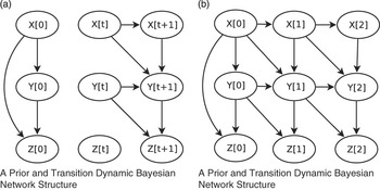
In order to model temporal processes, special structures are needed. This is because the arcs in a Bayesian network say nothing about time, only about probabilistic relationships. For these purposes, dynamic Bayesian networks (DBNs) are a useful representation. The key to DBNs is that they are specified in two parts, a prior Bayesian network that specifies the initial conditions and a transition Bayesian network that specifies how variables change from time to time. An example DBN, due to Friedman et al. (Reference Friedman, Murphy and Russell1998), is shown in Figure 6. In this, the prior and transition network are shown. It can be seen that while the prior network is simply a general Bayesian network, the transition network has slightly more structure to it. In this, there are two layers of nodes, and arcs from the first layer only go to the second. In addition, no arcs go from the second layer to the first. For the purposes of performing inference, or simply reasoning about them, DBNs can be expanded out into a single network. The network in Figure 6(a) has been expanded out in Figure 6(b) to a network of three layers. More information of DBNs can be found in the papers of Dean and Kanazawa (Reference Dean and Kanazawa1989) and Friedman et al. (Reference Friedman, Murphy and Russell1998) and in the work of Murphy and Mian (Reference Murphy and Mian1999). In addition, Ghahramani (Reference Ghahramani1998) examines the topic from the perspective of learning and Flesch and Lucas (Reference Flesch and Lucas2007) consider DBNs where the transition network can change over time.

Figure 6

Dynamic Bayesian network structures

1.5 Applications

This section aims to look at some typical applications of Bayesian networks. A lot of the original applications were in the medical field and to some extent, this is the domain where Bayesian network applications dominate today. However, there are now many uses in diverse domains, including biology, natural language processing and forecasting. Part of the popularity of Bayesian networks must stem from their visual appeal, as it makes them amenable to analysis and modification by experts. However, it is the generality of the formalism that makes them useful across a wide variety of circumstances. As a Bayesian network is a joint probability distribution, any question that can be posed in a probabilistic form can be answered correctly and with a level of confidence. Some examples of these questions are:

• • Given some effects, what were the causes?

• • How should something be controlled given current readings?

• • In the case of causal Bayesian networks, what will happen if an intervention is made on a system?

Below are examples of applications across many different domains that ask in one form or another, questions like those noted above. These examples are merely intended to show what is possible with Bayesian network modelling and the list is therefore intentionally short. For a more thorough treatment of the area, the recent book of Pourret et al. (Reference Pourret, Naïm and Marcot2008) show many examples of Bayesian networks in practice and for a nuts and bolts approach to modelling with Bayesian networks, the book by Kjaerulff and Madsen (Reference Kjaerulff and Madsen2008) goes into detail about the various subtle facets that surround this area.

Medicine. As noted previously, there are many applications of Bayesian networks in medicine. An overview of the field is given by Lucas et al. (Reference Lucas, van der Gaag and Abu-Hanna2004), but some of the more famous applications are given here.

An early implementation of a system for diagnosis in internal medicine was the quick medical reference (QMR). This system was reformulated in a Bayesian network implementation, with three levels of nodes; background, diseases and symptoms. Known as QMR-DT, it had a very large number of nodes and arcs (Middleton et al., Reference Middleton, Shwe, Heckerman, Henrion, Horvitz, Lehmann and Cooper1991; Shwe et al., Reference Shwe, Middleton, Heckerman, Henrion, Horvitz, Lehmann and Cooper1991). As a result, algorithms had to be developed that could perform inference in this dense network Shwe and Cooper (Reference Shwe and Cooper1991). Another more specific diagnostic system comes from the Pathfinder project (Heckerman et al., Reference Heckerman, Horvitz and Nathwani1992), which is used in the diagnosis of lymph-node diseases. In the same vein, though used for diagnosing neuromuscular disorders is the MUNIN network developed by Andreassen et al. (Reference Andreassen, Jensen, Andersen, Falck, Kjrul, Woldbye, Srensen, Rosenfalck and Jensen1989).

Within a similar domain, but used for a different purpose is the ALARM network developed by Beinlich et al. (Reference Beinlich, Suermondt, Chavez and Cooper1989), which was used for the monitoring of patients in intensive care situations. It is often treated as a gold-standard network, as it is reasonably well connected and has enough nodes to be a challenging, but still achievable problem for many Bayesian network algorithms. And from a learning perspective, Acid et al. (Reference Acid, de Campos, Fernandez-Luna, Rodriguez, Rodriguez and Salcedo2004) give a comparison of learning algorithms on the emergency medicine domain.

Forecasting. Bayesian networks can be very useful in predicting the future based on current knowledge. One of the most well known of these is the HailFinder network of Abramson et al. (Reference Abramson, Brown, Edwards, Murphy and Winkler1996), which is used to forecast severe weather. Also in the weather forecasting domain is the sea breeze prediction system of Kennett et al. (Reference Kennett, Korb and Nicholson2001), which uses learned structure and probability.

In the market domain, Abramson and Finizza (Reference Abramson and Finizza1991) use a Bayesian network to forecast oil prices, while Dagum et al. (Reference Dagum, Galper and Horvitz1992) show a dynamic Bayesian network used for the same task. And to the extent that classification can be seen as forecasting, Bayesian networks have huge potential. An example of this is by Friedman et al. (Reference Friedman, Geiger and Goldszmidt1997) who give a generalization of the high-performance Naïve-Bayes classifier into the tree-augmented Naïve-Bayes classifier. Other implementations of classification using Bayesian networks include those by Correa et al. (Reference Correa, Freitas and Johnson2007), who use them in the classification stage of an algorithm that also features attribute selection using a discrete particle-swarm optimization algorithm and Cheng and Greiner (Reference Cheng and Greiner1999) who compare classifiers of different complexity.

Control. An interesting use of DBNs in the control area is that of Forbes et al. (Reference Forbes, Huang, Kanazawa and Russell1995) who showcase their Bayesian automated taxi (BATmobile) network. This network is in the form of a dynamic influence diagram, and the system as a whole illustrates all the problems that must be solved to provide reliable control in a noisy, partially observed domain.

Modelling for human understanding. Friedman et al. (Reference Friedman, Linial, Nachman and Pe’er2000) and Friedman (Reference Friedman2004) look at modelling the causal interactions between genes by analysing gene expression data. They use the sparse candidate (SC) algorithm Friedman et al. (Reference Friedman, Nachman and Pe’er1999c) as described in Section 4.9.1 to learn the structure of 800 genes using 76 samples. These ideas have been built on by Husmeier (Reference Husmeier2003) and other researchers (Aitken et al., Reference Aitken, Jirapech-Umpai and Daly2005) who look at the problem of small sample sizes prevalent with biological data and examine techniques to characterize the sensitivity and specificity of results.

2.1 Introduction to inference

Inference in Bayesian networks generally refers to:

• • finding the probability of a variable being in a certain state, given that other variables are set to certain values; or

• • finding the values of a given set of variables that best explains (in the sense of the highest MAP probability) why a set of other variables are set to certain values.

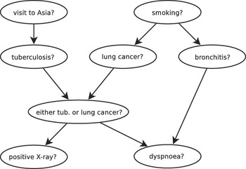
The Bayesian network structure in Figure 7 will be used to illustrate these problems. This is the well-known ASIA network, as defined by Lauritzen and Spiegelhalter (Reference Lauritzen and Spiegelhalter1988). With the first problem, a patient might present as a smoker and obtain a positive X-ray. Using this network, a physician might want to find out the probability that they have lung cancer, that is, P(lung cancer = true). With the second problem, a physician might want to find out the most probable explanation that explains these symptoms, that is, what is the most likely set of conditions (e.g. out of tuberculosis, lung cancer and bronchitis) that have caused the symptoms. In this article, it is generally the first problem that is being looked at, though the second will be mentioned as well. A recent article by Butz et al. (Reference Butz, Hua, Chen and Yao2009) describes a scheme to illustrate inference in Bayesian networks and while most inference algorithms supply a point value, recent work by Allen et al. (Reference Allen, Singh, Greiner and Hoope2008) show how it is possible to infer a distribution when the parameters themselves are seen as random variables.

Figure 7

The ASIA Bayesian network structure

2.2 Trees and polytrees

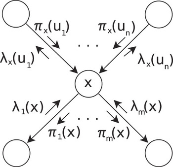
The first Bayesian network inference algorithms were developed for trees and polytrees, that is, Bayesian network structures that contained only a single path between any two nodes. Pearl (Reference Pearl1982) was the first to apply an inference procedure on trees, with Kim and Pearl (Reference Kim and Pearl1983) extending this to polytrees. The polytree algorithm was later extended by Peot and Shachter (Reference Peot and Shachter1991) to visit each node at most twice. Regardless of any speed-ups, Pearl’s message passing algorithm is important, as it operates in polynomial time with singly connected networks. An illustration of this scheme is shown in Figure 8. Here, each node is an autonomous processor that collects evidence from its n parents (π_x (u ₁), … , π_x (u _n)) and m children (λ ₁ (x), … , λ_m (x)), performs processing and sends out messages to its parents (λ_x (u ₁), … , λ_x (u_n)) and children (π ₁ (x), … , π_m (x)). The whole procedure is inherently asynchronous and is the basis of many of the inference schemes for multiply-connected networks.

Figure 8

Inference by message passing

2.3 Multiply-connected networks

A problem with Pearl’s algorithm is that it can only be applied to singly connected networks. Otherwise its messages can loop forever. Pearl (Reference Pearl1986b) reported on this problem and mentioned some techniques that can solve this, which are explained in the next sections. On account of the large number of possible techniques, the comparison of Díez and Mira (Reference Díez and Mira1994) is quite helpful.

The probable explanation for the plethora of inference methods is that Bayesian network inference is NP-hard in both the exact (Cooper, Reference Cooper1990) and approximate (Dagum & Luby, Reference Dagum and Luby1993) case, where the network is multiply connected. The following techniques seek to cut down the possibly exponential time needed.

2.4 Clustering

One of the first methods to help apply the message passing algorithm to multiply-connected networks was by Spiegelhalter (Reference Spiegelhalter1986). In this he describes a way of ‘pulling loops together’, into clusters. These clusters are then joined together into a singly connected structure, and a message-passing algorithm is started. This is built upon by Lauritzen and Spiegelhalter (Reference Lauritzen and Spiegelhalter1988) and then by Jensen et al. (Reference Jensen, Lauritzen and Olesen1990a, Reference Jensen, Olesen and Andersen1990b), who describe a variant of the clustering algorithm that builds a so-called junction tree. They later give an optimal algorithm for junction tree construction given a triangulated graph (Jensen and Jensen, Reference Jensen and Jensen1994).

Later authors looked into trying to optimize junction tree inference. Breese and Horvitz (Reference Breese and Horvitz1991) show how to trade off time spent on decomposition of the Bayesian network against actual inference. Other authors examine ways to get an optimal decomposition, for example, Kjærulff (Reference Kjærulff1992b) uses simulated annealing, Gámez and Puerta (Reference Gámez and Puerta2002) use ant colony optimization in building the tree and Huang and Darwiche (Reference Huang and Darwiche1996) show how best to implement clustering. Some useful bounds have been found by Becker and Geiger (Reference Becker and Geiger2001, Reference Becker and Geiger1996b), who present an algorithm that is sufficiently fast for building close to optimal junction trees.

Other authors have looked at the structure of the clique tree; Kjærulff (Reference Kjærulff1997) shows how the cliques in the tree may themselves be factored into a clique tree, and Darwiche (Reference Darwiche1998) shows how to keep clique trees up to date after pruning irrelevant parts of the network.

A clustering architecture that differs slightly from Lauritzen and Spiegelhalter, and Jensen et al. is that of Shenoy and Shafer (Reference Shenoy and Shafer1990) and Shafer and Shenoy (Reference Shafer and Shenoy1990). It is worth noting, as it has been used by various authors, albeit to a lesser degree than the other schemes, for example, by Shenoy (Reference Shenoy1997) and Schmidt and Shenoy (Reference Schmidt and Shenoy1998).

2.5 Variable elimination and arc reversal

A simple method of inference involves reversing arcs in a Bayesian network and removing variables. Shachter (Reference Shachter1986a, Reference Shachter1986b) introduced this in the context of evaluating influence diagrams—Bayesian networks that have decision and utility nodes that recommend a course of action to follow. This idea is continued on by Shachter (Reference Shachter1988). It is useful to note that the node removal method of Zhang and Poole (Reference Zhang and Poole1994b) proceeds from a different angle than Shachter.

2.6 Conditioning

Another one of the original techniques used to perform inference in multiply-connected networks was that of conditioning. In this procedure, loops in the network are broken by instantiating nodes and the message passing algorithm is run on the singly connected networks, one for each combination of values that the nodes take on. Pearl (Reference Pearl1986a) was the first to use this method, while Suermondt and Cooper (Reference Suermondt and Cooper1988, Reference Suermondt and Cooper1990) show the optimal cutset is NP-hard to find. One issue with conditioning is that the set of nodes that cut the loops (the cutset) need to have a joint prior probability assigned to them; Suermondt and Cooper (Reference Suermondt and Cooper1991) have a method to handle this.

As conditioning is NP-hard, it is good to know that Becker and Geiger (Reference Becker and Geiger1994, Reference Becker and Geiger1996a) have an algorithm (MGA) that finds a loop cutset with a guaranteed cardinality of less than twice the minimum cardinality. Other researchers have designed methods to try to alleviate the problems of conditioning; for more information see, for example, Díez (Reference Díez1996), Shachter et al. (Reference Shachter, Andersen and Szolovits1994) and Darwiche (Reference Darwiche1995, Reference Darwiche2001b).

2.7 Symbolic probabilistic inference

Li and D’Ambrosio (Reference Li and D’Ambrosio1994) have found a method that splits the task of inference into two parts. First, a symbolic factorization of the joint probability distribution based on the Bayesian network is found. Then a numeric step is performed where the actual probabilities are calculated. This style of inference has been built on by Chang and Fung (Reference Chang and Fung1995), who look at continuous variables and by Castillo et al. (Reference Castillo, Gutiérrez and Hadi1995, Reference Castillo, Gutiérrez and Hadi1996) who develop a slightly different system for the symbolic inference.

2.8 Polynomial compilation

A recent technique by Darwiche (Reference Darwiche2003) and Park and Darwiche (Reference Park and Darwiche2004) shows that Bayesian networks can be represented as a polynomial. Probabilistic queries can be formulated by evaluating and differentiating this polynomial. This is based on the fact that every Bayesian network is a multi-linear function, which can be encoded in decomposable negation normal form (d-DNNF; Darwiche, Reference Darwiche2001a), a language for representing propositional statements that has useful properties for evaluation. This can then be implemented as an arithmetic circuit (Darwiche, Reference Darwiche2002), which is easy to evaluate and differentiate.

The inference of Bayesian networks as polynomials is interesting, as it can be shown that they subsume other methods of inference such as clustering. They can also be more efficient than other methods that have been discussed, such as clustering and conditioning, as the compilation phase of the method can be performed offline and optimizations performed (Chavira & Darwiche, Reference Chavira and Darwiche2007).

2.9 Monte Carlo methods

As inference in Bayesian networks was found to be NP-hard in general (Cooper, Reference Cooper1990), attention was paid to heuristic and stochastic techniques to help solve the problem. It was then found that approximate inference is also NP-hard (Dagum & Luby, Reference Dagum and Luby1993). However, in general, approximate inference techniques have a wider range of applicability on hard networks than exact techniques. Some of the most prevalent inexact techniques are based on Monte Carlo methods; the paper of Cousins et al. (Reference Cousins, Chena and Frisse1993) has a short tutorial on the subject in relation to Bayesian network inference, whereas the paper of Dagum and Horvitz (Reference Dagum and Horvitz1993) analyses the performance of simulation algorithms using a Bayesian perspective.

2.10 Other approximate inference

As well as sampling-based approaches, inference in Bayesian networks may be tackled using other, more heuristic methods. These include search-based methods, model simplification methods and ones based on the loopy belief propagation idea, which will be explained later. A comparison of sampling and search-based algorithms in approximate inference can be found in the work of Lin and Druzdzel (Reference Lin and Druzdzel1999).

2.11 Inference in dynamic Bayesian networks

Inference in DBNs often needs a special approach to deal with their particular structure. Although a transition DBN can be represented as a finite number of time slices (normally two), inference in general needs to be computed over the expanded network; that is, inference needs to compute at a particular time. Apart from the possibly massive number of nodes if the time is far in the future, the repetitious structure of this expansion is often not amenable to standard exact techniques for multiply-connected networks; see Boyen and Koller (Reference Boyen and Koller1998) for a look at this problem and a possible solution. Kjærulff (Reference Kjærulff1992a) looks at reasoning in dynamic Bayesian networks, based on Lauritzen and Spiegelhalter’s approach, while Ghahramani and Jordan (Reference Ghahramani and Jordan1997) use variational approximations on factorial hidden Markov models (a subtype of DBNs) and Jitnah and Nicholson (Reference Jitnah and Nicholson1999) also use approximations by pruning. Meanwhile, Kanazawa et al. (Reference Kanazawa, Koller and Russell1995) adapt standard sampling techniques to the ‘special characteristics’ of DBNs.

2.12 Causal-independence networks

Bayesian networks are often specified, where all parents of a node are independent of each other. This can happen if the network was constructed by hand, or if in the course of structure learning, prior knowledge specified that this should be the case. Therefore, inference procedures need to be aware of this possible situation. An advantage is that causal-independence models can reduce inference complexity (Zhang & Poole, Reference Zhang and Poole1994a).

Inference in causal-independence networks has been performed since Kim and Pearl (Reference Kim and Pearl1983) specified their extension of Pearl’s message passing scheme. From then on, authors have developed different methods of representing causal independence and how to perform inference and learning. For example, Zhang and Poole (Reference Zhang and Poole1996) examine methods involving an operator acting upon the effects of a nodes parents, for example, or, sum or max. Jaakkola and Jordan (Reference Jaakkola and Jordan1996) look at computing upper and lower bounds on likelihoods in sigmoid and noisy-OR networks. Huang and Henrion (Reference Huang and Henrion1996) also investigate noisy-OR inference with their TopEpsilon system. Other interesting papers on the subject include those by Heckerman and Breese (Reference Heckerman and Breese1996), Boutilier et al. (Reference Boutilier, Friedman, Goldszmidt and Koller1996) and Zhang and Yan (Reference Zhang and Yan1998).

3.1 Multinomial data

A multinomial variable is a variable that can take on one of a finite number of possible values. Any data corresponding to a multinomial variable is known as multinomial data. When dealing with multinomial data, there are choices that can be made as to how the learning is to proceed. Perhaps one of the simplest methods is to estimate the parameters of the model using a maximum likelihood approach. However, this has a problem with sparse data, in that some probabilities—perhaps most of them—can be undefined if a case does not come up in the database. This can cause problems later with inference. To counteract this, some form of prior distribution is normally placed on the variables, which is then updated from the data. An example of this would be a distribution that said all values of a particular variable were of an equal prior probability to begin with, but changed quickly to reflect the observed data. Heckerman and Geiger (Reference Heckerman and Geiger1995) and Buntine (Reference Buntine1996) discuss this more. In addition, under certain reasonable assumptions—that the parameters of the network are independent of each other and the density function characterizing each parameter is strictly positive—Geiger and Heckerman (Reference Geiger and Heckerman1995, Reference Geiger and Heckerman1997) showed that this distribution must be Dirichlet. The Dirichlet distribution is the multivalued generalization of the Beta distribution and is a conjugate prior of the multinomial; that is, when updated with new information, the updated distribution is again Dirichlet. As an example, the form of the Beta density function is given by

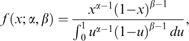
for parameters α and β and variable x. When a series of Bernoulli trials is performed, with s successes and t failures and a prior given by f (x; α, β) is specified, the posterior distribution is given by f (x; α + s, β + t). This allows easy extraction of statistics and in the case of complete data, a simple closed form updating rule. These ideas are expanded upon by Castillo et al. (Reference Castillo, Hadi and Solares1997b), while Burge and Lane (Reference Burge and Lane2007) show another way of smoothing the maximum likelihood estimates.

3.2 Continuous variables

Although a lot of the literature on Bayesian networks assumes that the data are multinomial, for many applications, the data supplied are continuous and therefore ways must be found to handle this situation. While the simplest method might be to discretize the data as done by Monti and Cooper (Reference Monti and Cooper1998), this can cause problems. However, there exist methods for representing continuous data under different assumptions. One of the first of these assumptions is that the data are normally distributed. Geiger and Heckerman (Reference Geiger and Heckerman1994) use this to learn using continuous data. Taking away the normal assumption, Hofmann and Tresp (Reference Hofmann and Tresp1996) use kernel density estimators to model the conditional distribution. These two methods are compared by John and Langley (Reference John and Langley1995), who show that the non-parametric approach of kernel density estimators can be useful. Another non-parametric way of estimating the conditional densities is given by Monti and Cooper (Reference Monti and Cooper1997a), who use neural networks in this regard. They also look at the situation of hybrid networks, that is, Bayesian networks with continuous and discrete attributes.

3.3 Missing data/hidden variables

One large problem in learning Bayesian networks, and indeed in running any machine learning algorithm is dealing with missing data, a problem that occurs in perhaps most real-life data sets. There are generally three different missing data assumptions that can be applied to missing data. Under a missing-completely-at-random (MCAR) assumption, the missing value mechanism depends neither on the observed data nor on the missing data. This means that the data with missing values could simply be discarded. This is an extremely easy situation to implement, but is a bad policy in general, in that some if not most of the data would be unavailable for learning. Under a missing-at-random (MAR) assumption, the missing value mechanism depends on the observed data. This means the missing data can be estimated from the observed data. This is more complicated than the MCAR situation, but all the data get used. Under a missing-not-at-random (MNAR) assumption, the missing value mechanism depends on both the observed and missing data. On account of this, a model of the missing data must be supplied. This is the most complicated situation, as a model may not be readily available, or could even be unknown.

3.4 Miscellaneous techniques

This section will show some techniques in learning parameters that look at specific topics.

First, researchers have looked at learning parameters in causal independence models, that is, models where causes can be assumed to be independent from each other, for example, in noisy-OR and noisy-MAX nodes. Meek and Heckerman (Reference Meek and Heckerman1997) show how these types of nodes can be learned using Bayesian methods, while Neal (Reference Neal1992) shows learning noisy-OR and sigmoid models using Gibbs sampling.

The simplest model of a multinomial conditional probability distribution is probably representing it as a table of values. However, other representations may be possible, such as trees, that can model non-interactions between variables at a finer level. For example, Friedman and Goldszmidt (Reference Friedman and Goldszmidt1996b) demonstrate simple algorithms that can learn conditional probability distributions as tables or trees, as part of an overall structure learning algorithm. In the same vein, Chickering et al. (Reference Chickering, Heckerman and Meek1997a, Reference Chickering, Heckerman and Meek1997b) show an algorithm that learns decision graphs for the CPDs as well as the network structure and desJardins et al. (Reference desJardins, Rathod and Getoor2008) also show how to learn tree-structured parameters and structures together.

In regards to learning dynamic Bayesian networks, Ghahramani and Jordan (Reference Ghahramani and Jordan1997) discuss learning the parameters of a factorial hidden Markov model (and hence a specific type of dynamic Bayesian network). This is generalized to DBNs and an analysis is done over many different specializations of DBNs (Ghahramani, Reference Ghahramani1998).

Normally, updating parameters in an online setting is not a hard task, but when coupled with structure learning, there can be difficulties in knowing what data to remember. An early look at this problem is given by Buntine (Reference Buntine1991), who describes a system of keeping possible parameters for a node in a lattice structure. Bauer et al. (Reference Bauer, Koller and Singer1997) look at a different problem, with updating parameters in an online setting, assuming missing data.

There has not been much discussion on the use of prior knowledge in learning parameters, so the paper by Feelders and van Straalen (Reference Feelders and van Straalen2007) is interesting. It shows how an expert can give an indication of qualitative influence of parent variables on a child and how this can increase the accuracy of parameter estimation.

Finally, the papers below represent some interesting ideas in parameter learning, with possible applications to structure learning. As a prelude to their structure learning method described in Section 4.16, Tong and Koller (Reference Tong and Koller2001a) present an application of using active learning to estimate parameters in a Bayesian network. Also in the context of structure learning, Greiner et al. (Reference Greiner, Grove and Schuurmans1997) examine ways of learning CPDs dependant on the queries that will be put to the network.

4.1 Learning theory and learning complexity

There is a lot of theory behind the learning of Bayesian networks, most of which is rooted in statistical concepts and graph theory. Geiger et al. (Reference Geiger, Heckerman, King and Meek2001) and Geiger (Reference Geiger1998) look at different families of models (of which Bayesian networks are one) in the context of model selection, but a gentler introduction can be found in the pages of the books of Pearl (Reference Pearl1988), Jensen and Nielsen (Reference Jensen and Nielsen2007), Castillo et al. (Reference Castillo, Gutiérrez and Hadi1997a) and Cowell et al. (Reference Cowell, Dawid, Lauritzen and Spiegelhalter1999). From a more recent perspective, Kočka et al. (Reference Kočka, Bouckaert and Studený2001) and Castelo and Kočka (Reference Castelo and Kočka2003) investigate the important role of inclusion in learning Bayesian network structure (i.e. whether the conditional independence statements in one structure are a subset of those in another). And while the theory of learning is important as a basis to why certain techniques are adopted, to many people, the issue of complexity of learning is the most immediately obvious challenge.

4.2 Causal networks

Bayesian networks can have a number of interpretations depending on the use they will be put to and the background of the people constructing them. At its most basic, a Bayesian network is a factorization of a joint probability distribution, with properties that make storage and inference convenient. In this construction, the arcs between nodes characterize the probabilistic dependencies between variables and how the associated conditional probability distributions are combined.

Another view is that a Bayesian network represents causal information, with the arcs representing direct causal influences, such that manipulating a variable at the tail of an arc will cause a change to occur with the variable at the head of the arc in almost all circumstances. This interpretation is more controversial as it goes against the grain of conventional statistical wisdom that says that causality can only be found using manipulation. Although causal Bayesian networks are controversial, they are a tempting objective for a number of reasons. For one, being able to learn a causal network can provide insight into a domain. And from a computational perspective, a causal network allows the effect of interventions and not just observations to be computed. It is worth noting that while Bayesian networks have been seen by many as the best way to represent uncertain causal knowledge, recent work has put forward generalizations of Bayesian networks as being better able to handle the subtle issues of causal reasoning (Richardson & Spirtes, Reference Richardson and Spirtes2002; Zhang, Reference Zhang2008).

There are many pitfalls to be wary of when learning causal networks. These include (but are not limited to), hidden common causes, selection bias and feedback loops. Use of machine learning methods to learn causal Bayesian networks from data means that assumptions are being made (implicit or explicit), such as the causal Markov condition or faithfulness condition (Spirtes et al., Reference Spirtes, Glymour and Scheines2000), though new research has indicated possible weaker assumptions (Zhang & Spirtes, Reference Zhang and Spirtes2008). There has been much confusion over when utilizing causal networks is applicable (Druzdzel & Simon, Reference Druzdzel and Simon1993). Many studies (probably wrongly) have assumed that Bayesian networks and causal Bayesian networks are equivalent (Acid & de Campos, Reference Acid and de Campos1995; Acid et al., Reference Acid, de Campos and Huete2001); more careful studies set out their assumptions clearly beforehand. Most of the work in learning causal networks has focused on constraint-based algorithms, building on work from Glymour et al. (Reference Glymour, Scheines, Spirtes and Kelly1986), Spirtes et al. (Reference Spirtes, Glymour and Scheines1989, Reference Spirtes, Glymour and Scheines1990) and Spirtes and Glymour (Reference Spirtes and Glymour1990a, Reference Spirtes and Glymour1991) and also work from Geiger et al. (Reference Geiger, Paz and Pearl1990), Pearl and Verma (Reference Pearl and Verma1991) and Verma and Pearl (Reference Verma and Pearl1991, Reference Verma and Pearl1992). However, there also have been studies on learning causal structures from a score and search perspective, particularly within a Bayesian framework (Heckerman, Reference Heckerman1995a, Reference Heckerman2007). There have been many works on causal Bayesian networks, but the two most relevant are probably those by Spirtes et al. (Reference Spirtes, Glymour and Scheines2000) and Pearl (Reference Pearl2000) who expound their views on the possibilities of the topic. These must be contrasted against the debates of philosophers on the ability of Bayesian networks to capture causal information. Prominent papers in this area include those of Cartwright (Reference Cartwright2001), exchanges between Hausman and Woodward (Reference Hausman and Woodward1999, Reference Hausman and Woodward2004) and Cartwright (Reference Cartwright2002, Reference Cartwright2006), and contributions by Williamson (Reference Williamson2005) and Steel (Reference Steel2005, Reference Steel2006).

4.3 Trees

One of the first pieces of work on learning structure was by Chow and Liu (Reference Chow and Liu1968), who described an algorithm for learning Bayesian networks structured as trees, that is, a structure where each node has either one or zero parents. These are sometimes known as Chow–Liu trees. Their algorithm constructs the optimal second-order approximation to a joint distribution, by finding the maximal spanning tree, where each branch is weighted according to the mutual information between the two variables. This work was built upon by Ku and Kullback (Reference Ku and Kullback1969) who demonstrate that it is a special case of a more general framework to approximating joint probability distributions.

There has continued to be research on trees as a decomposition of a joint distribution, for example, by Lucas (Reference Lucas2002) and Friedman et al. (Reference Friedman, Geiger and Goldszmidt1997) in the context of classification. Meil and Jaakkola (Reference Meilaˇ and Jaakkola2006) show how learning tree structures in a fully Bayesian manner can be achieved in polynomial time.

4.4 Polytrees

More general than trees, polytrees are an important class of Bayesian network structure. A polytree is a graph in which there are no loops, irrespective of arc direction. They are important because there exist exact algorithms that can perform inference on the polytree in polynomial time (Kim & Pearl, Reference Kim and Pearl1983; Peot & Shachter, Reference Peot and Shachter1991).

One of the earliest examples on learning polytrees from data is given by Pearl (Reference Pearl1988), following on from work by Rebane and Pearl (Reference Rebane and Pearl1987), which uses Chow and Liu’s (Reference Chow and Liu1968) system as a subroutine. Dasgupta (Reference Dasgupta1999) gives a good look at the field and mentions the NP-hardness of the problem, while showing a good approximation and de Campos (Reference de Campos1998) looks at what properties a dependency model must have in order to be represented by a polytree. Other work on the area includes Geiger et al. (Reference Geiger, Paz and Pearl1990), Acid and de Campos (Reference Acid and de Campos1995), who show an empirical study into approximating general Bayesian networks by polytrees and Huete and de Campos (Reference Huete and de Campos1993) who look at using conditional independence tests (see Section 4.8) to learn polytrees.

We will now turn our attention to the problem of learning a general Bayesian network structure, that is, a DAG. This has by far received the most attention from the research community and correspondingly there are many more publications. In the sections that follow, there will be a classification of the various factors involved, but it is worthwhile to bear in mind that some ideas fall into many different camps.

4.5 Heuristic algorithms

One of the most widely studied ways of learning a Bayesian network structure has been the use of so-called ‘score-and-search’ techniques. These algorithms comprise of:

• • a search space consisting of the various allowable states of the problem, each of which represents a Bayesian network structure;

• • a mechanism to encode each of the states;

• • a mechanism to move from state to state in the search space; and

• • a scoring function to assign a score to a state in the search space, to see how good a match is made with the sample data.

Because of the hardness of the problem, heuristic algorithms are generally used to explore the search space, the most basic of which are greedy searches (GSs). In all these frameworks, it is useful to bear in mind the work of Xiang et al. (Reference Xiang, Wong and Cercone1996), who show that single-link search cannot find all models.

4.6 Searching through the space of equivalence classes

As the structure of a Bayesian network is a DAG, it is natural to use this representation as a state while searching through the space of possible structures. However, it has been noted that certain DAGs are similar in that they capture the same conditional independencies in their structure (Andersson et al., Reference Andersson, Madigan and Perlman1997). These Markov equivalent structures have been discussed in Section 1.3. Since the CPDAG structure discussed in that section can represent an equivalence class of DAG structures, it is very useful in representing states of searches. The space of these searches can be known as E-space, as opposed to the B-space of DAG-based search (Chickering, Reference Chickering2002a). More information on these topics can be found in Lauritzen and Wermuth (Reference Lauritzen and Wermuth1989) and Whittaker (Reference Whittaker1990).

4.7 Scoring functions

When performing a score-and-search procedure a scoring criterion must be specified that somehow gives a good score when a structure matches the data ‘well’—the better the match, the higher the score. Of course, given this ambiguous problem, diverse scoring criteria have been invented that involve various assumptions and different definitions of a better match. Perhaps one of the simplest criterion—the maximum likelihood estimator—will in general return the complete graph, as this is the one with the most parameters. Therefore, most scoring criteria consist of two parts—one that rewards a better match of the data to the structure and one that rewards a simpler structure. Examples of these are the Bayesian Dirichlet (BD) criterion, Bayesian information criterion (BIC), Akaike information criterion (AIC), MDL and minimum message length (MML). These and various other criteria will be discussed below.

One of the more desirable properties of a scoring criterion is decomposability, whereby the score of a particular structure can be obtained by the score for each node given its parents. Most of the scoring functions known have this property. Malvestuto (Reference Malvestuto1991) has some early work on this.

A comparison of MDL, BDeu (BD with ) and K2 (BD with ) is given in Shaughnessy and Livingston (Reference Shaughnessy and Livingston2005). Note that in this paper, they confuse BDeu with K2 and the WEKA Bayesian method with BDeu. Another thorough comparison between the BIC, Cheeseman–Stutz approximation (Cheeseman & Stutz, Reference Cheeseman and Stutz1996), Laplace approximation and Gibbs sampling approach was conducted by Chickering and Heckerman (Reference Chickering and Heckerman1997). Finally a comparison between the MML and BGE metrics is given by Neil and Korb (Reference Neil and Korb1999).

4.7.1 Bayesian Dirichlet scoring functions

One of the first expositions of a Bayesian scoring criterion in learning Bayesian network structure was given by Cooper and Herskovits (Reference Cooper and Herskovits1992) as part of their K2 algorithm. As presented by them, the function for a given structure B_s and data set D were

where there are n variables, q_i parent configurations of variable i, r_i is the number of values variable i can take, N_ijk is the number of times variable, i took on value k with parent configuration j and . Looking at this equation it can be seen that P(B_s) is the prior probability of structure B_s and the rest of the expression is the likelihood of the structure, given the data.

In their paper, Heckerman et al. (Reference Heckerman, Geiger and Chickering1995) generalize the above equation and place it on a sound theoretical footing. In their form,

where variables have the same meaning as before and are exponents that specify the users prior knowledge about configuration ijk; the higher the , the more the user thinks that configuration is likely. Meanwhile, . They called this equation the Bayesian Dirichlet or BD metric. It can be noted that Γ(x) = (x−1)! for natural numbers, which immediately shows the similarity to the equation of Cooper and Herskovits (Reference Cooper and Herskovits1992). Indeed, with , the formula is exactly the same as the K2 formula. Using an assumption known as likelihood equivalence, which says that equivalent structures receive the same score, they constrain the values that can take on and provide a method to calculate them. With this method, the user provides a prior Bayesian network and an equivalent sample size N′ that says how confident they are in it. With these constraints, the scoring criterion is named BDe (Bayesian Dirichlet with likelihood equivalence). With a further constraint, such that all configurations are as likely as each other, and the criterion is named BDeu (Bayesian Dirichlet with likelihood equivalence and a uniform joint distribution). It would be well to note that the learned network can be quite sensitive to the N′ parameter (Steck & Jaakkola, Reference Steck and Jaakkola2003a; Silander et al., Reference Silander, Kontkanen and Myllymaki2007), so recent work on optimizing it is welcome (Steck, Reference Steck2008).

4.7.2 Minimum description length

MDL is a statistical principle, which says that the best hypothesis that describes data, is the one that leads to the largest compression of that data, including the hypothesis (Rissanen, Reference Rissanen1978). One of the first people to use the MDL principle in constructing Bayesian networks was Bouckaert (Reference Bouckaert1993, Reference Bouckaert1994a). Here he provides an explanation and justification of using this measure and shows how it behaves like the K2 criterion for large sample sizes. A more in-depth comparison of the MDL and K2 criterion is given in Bouckaert (Reference Bouckaert1994b).

At around the same time, Suzuki (Reference Suzuki1993) and Lam and Bacchus (Reference Lam and Bacchus1994a) also made use of the MDL principle and presented a way to incorporate domain knowledge into their algorithm (Lam & Bacchus, Reference Lam and Bacchus1993). This domain knowledge can come in the form of direct causation information (X is a direct cause of Y) and a partial ordering of the variables. Suzuki (Reference Suzuki1999) looks into previous work using MDL and presents a branch-and-bound algorithm. Finally, Cruz-Ramírez et al. (Reference Cruz-Ramírez, Acosta-Mesa, Barrientos-Martnez and Nava-Fernández2006) give a comparison of MDL and BIC. In this work BIC is defined as

where are the maximum likelihood parameters for B_s, d is the number of free parameters in the model and n is the sample size. Following this, MDL is defined as

where k is the number of variables, and is the size of the parent set of variable x_i. Hence, according to Cruz-Ramírez et al., MDL is BIC with an extra penalty for model complexity. Note that some authors use the term MDL to mean the formula indicated by BIC above, so care must be taken to see exactly what is being used.

4.7.4 Other

Although the scoring criteria given above are the most widely used in the field, researchers have been examining other methods of ranking a structure given some data. For example, Kayaalp and Cooper (Reference Kayaalp and Cooper2002) introduce a scoring metric called Global Uniform (GU) that is based on a particular form of default parameter prior. They then compare it against the BDeu and K2 scoring criteria. de Campos (Reference de Campos2006) presents a scoring method called mutual information tests that has an information theoretic basis and performs well compared to K2, BDeu, BIC and the PC algorithm of Spirtes and Glymour (Reference Spirtes and Glymour1990a). Also based on information theory, the work of Herskovits and Cooper (Reference Herskovits and Cooper1991) uses a scoring function that calculates the entropy of a particular network, with the network of minimum entropy being the best fit to the data. Their decomposable function is

Based upon this they show a method to calculate the best arc to add to the network being generated. Recently, Riggelsen (Reference Riggelsen2008) describes a new Bayesian scoring function that does not make the Dirichlet assumption and attempts to learn both the structure and parameters together.

An interesting approach with similarities to boosting, etc. is that by Elidan et al. (Reference Elidan, Ninio, Friedman and Schuurmans2002) who reweighted data, so that the scoring function can change. This can help escape local maxima. Castelo and Perlman (Reference Castelo and Perlman2002) demonstrate a scoring criterion that can be applied directly to equivalence classes of Bayesian network structures, without extending it to DAG form.

4.8 Finding structure using conditional independencies

In learning the structure of a Bayesian network from data, there are often said to be two main methods—search through the space of possible structures and using conditional independencies (CIs) obtained from statistical tests on the data. In this section, the latter will be focused on. However, it is worth noting that Cowell (Reference Cowell2001) has drawn parallels between the two techniques, so they might not be as different as they seem at first glance. Perhaps the book for learning using CIs is the one by Spirtes et al. (Reference Spirtes, Glymour and Scheines1993, Reference Spirtes, Glymour and Scheines2000), which contains most of the early theory and results, and looks at the problem from a causal perspective.

Some of the first work on using CIs to obtain structure came from around the early 1990s. Geiger et al. (Reference Geiger, Paz and Pearl1990) developed an algorithm to recover polytrees from an oracle, which can say whether two variables are independent given another. At the same time Fung and Crawford (Reference Fung and Crawford1990) developed the Constructor system that learned Markov networks, that is, undirected graphical models, that encode CIs in a manner similar to Bayesian networks. In this work, they mention using the χ ² statistical test to obtain the needed CIs.

One of the first systems that recovered a DAG from independence data was the SGS algorithm by Spirtes et al. (Reference Spirtes, Glymour and Scheines2000). However, this was quite inefficient, as each pair of variables required tests involving every subset of the remaining variables, which is an exponential operation. Therefore, numerous variations on the theme sprung up. Perhaps the best known of these is the PC algorithm by Spirtes and Glymour (Reference Spirtes and Glymour1990a), which is faster than SGS, but can produce errors in removing arcs. These arise because PC only tests for d-separation between nodes X and Y in a DAG, using subsets of neighbours of X and Y. A modification of the PC algorithm that decreases the amount of Causal Inference (CI) tests needed is called PC* (Spirtes et al., Reference Spirtes, Glymour and Scheines2000), and recently, applicability of PC to high-dimensional data is shown by Kalisch and Bühlmann (Reference Kalisch and Bühlmann2007). Also recently, Li and Wang (Reference Li and Wang2009) show how to control the false positive rate while using the PC algorithm.

A variant of the SGS algorithm, proposed by Pearl and Verma (Reference Pearl and Verma1991) and Verma and Pearl (Reference Verma and Pearl1991), differs from previous approaches in that it first generates an undirected graph that models dependencies between variables, as opposed to using the complete undirected graph in the SGS and PC manner. This algorithm, called Inductive Causation (IC), also takes into account latent variables, and returns a graph with undirected, unidirected and bidirected arcs. Taking inspiration from the approach of IC in starting with the undirected independence graph, Spirtes et al. (Reference Spirtes, Glymour and Scheines2000) proposed changing the PC algorithm to start in the same way. They called this modified algorithm Independence Graph (IG). Again, with an approach based on IC, Verma and Pearl (Reference Verma and Pearl1992) looked at an algorithm that took a more global view and constructed a DAG, as opposed to the local view of IC.

Following on from the work of Verma and Pearl, Spirtes et al. (Reference Spirtes, Glymour and Scheines2000) described two algorithms that took on the idea of identifying latent variables. These were known as the CI and Fast Causal Inference (FCI) algorithms and Spirtes et al. (Reference Spirtes, Meek and Richardson1995) show how they can also work in the presence of, and identify, selection bias.

After the large body of work produced by Spirtes, Glymour and Scheines, and Verma and Pearl, various other authors examined ways to learn causal explanations of data in the context of DAGs. These are refinements of the more general approaches discussed above and were often developed for simplified situations. Cooper (Reference Cooper1997) described an algorithm called Local Causal Discovery (LCD) based on PC and FCI, that while less general in its applicability, runs in polynomial time in the worst case. de Campos (Reference de Campos1998) looked at representing CI statements using polytrees and developed algorithms for this purpose. de Campos and Huete (Reference de Campos and Huete1997) also make a simplifying assumption with their CH1 and CH2 algorithms that can efficiently find simple graphs; that is, DAGs where every pair of nodes with a child are not connected, nor have a common ancestor. Various authors also advanced systems that allow background knowledge to be given. For example, Meek (Reference Meek1995) showed a method for learning a CPDAG using methods inspired by Spirtes et al. This was done in the context of background knowledge in the form of mandatory and disallowed causal effects. This paper also has early work on finding DAGs from CPDAGs. Cheng et al. (Reference Cheng, Bell and Liu1997) have a system that takes an ordering of the variables as background knowledge, as do de Campos and Huete (Reference de Campos and Huete2000b), who describe a method that avoids making many high-order CI tests.

An interesting modification to the standard CI type algorithm is given by Margaritis and Thrun (Reference Margaritis and Thrun2000) with their GS algorithm, which shows how to limit the number of CI tests between two nodes by only using nodes in their Markov boundaries, which are calculated beforehand. Another interesting approach is that of Cheng et al. (Reference Cheng, Greiner, Kelly, Bell and Liu2002) and their three-phase dependency analysis (TPDA), who describe how an n variable DAG can be learned in O(n ⁴) CI tests. This was also implemented in parallel by Gou et al. (Reference Gou, Jun and Zhao2007). However, TPDA relies on an assumption known as monotone DAG-faithfulness, and it has been shown by Chickering and Meek (Reference Chickering and Meek2006) to be incompatible with the faithfulness assumption. They show that the optimality guarantee provided by Cheng et al. only applies in very specific situations, where there are already faster algorithms.

Some recent work on reducing computation time and errors in reconstructing networks is given by Yehezkel and Lerner (Reference Yehezkel and Lerner2006). They propose an algorithm known as recursive autonomy identification (RAI), that recursively performs CI tests, edge directions and structure decomposition, with higher order CI tests for smaller structures. Another recursive system is that of Xie and Geng (Reference Xie and Geng2008) that splits the variables into two sets recursively, builds a DAG when a set cannot be split anymore and combines these DAGs on returning from a split. More recent work by Bromberg and Margaritis (Reference Bromberg and Margaritis2009) describes how to use a logical process known as argumentation to resolve inconsistencies that can occur when a small sample size is used.

With all the algorithms given above, access to fast CI tests is crucial. The normal tests used are the χ ² and G tests (Spirtes et al., Reference Spirtes, Glymour and Scheines2000, pp. 93–95), but work has been done on a new test by Dash and Druzdzel (Reference Dash and Druzdzel2003). Other results concerning d-separations are given by Acid and de Campos (Reference Acid and de Campos1996a, Reference Acid and de Campos1996b), who use them in their hybrid BENEDICT system (Acid & de Campos, Reference Acid and de Campos1996c).

Finally, authors have used CI testing in ways that differ from the approach given above (using the conditional independencies to construct a dependency structure that is necessary in a candidate DAG). Examples of these are de Campos (Reference de Campos2006) who uses CI tests in the construction of a scoring function and Schulte et al. (Reference Schulte, Luo and Greiner2007) who provide a look at learning BN structures using CI tests in a paradigm that approaches the task using Gold’s learning paradigm (Gold, Reference Gold1967).

4.9 Hybrid search strategies

Both the score-and-search and conditional independence testing methods have their advantages. Score-and-search typically works better with less data than CI testing and with probability distributions that admit dense graphs. They also allow probability distributions over models to be easily represented and have better mechanisms for dealing with missing data. However, CI testing methods work well with sparse graphs, are generally quick and have good ways of finding hidden common causes and selection bias.

As both methods have advantages inherit in them, researchers have tried to find ways to use the good points of both in hybrid methods. Below are some of the ideas that researchers have been looking at.

4.10 Searching over orderings

Score-and-search algorithms for finding Bayesian network structures generally search over the space of DAGs and in some cases, the space of equivalence classes of DAGs. However in some cases, other spaces can be used. One that has received some attention is searching in the space of orderings.

Early papers on this subject were given by Larrañaga et al. (Reference Larrañaga, Kuijpers, Murga and Yurramendi1996a) as seen in Section 4.5.3 and by Wallace and Korb (Reference Wallace and Korb1999) who use an MCMC sampling procedure. Acid et al. (Reference Acid, de Campos and Huete2001) use an approach similar to Singh and Valtorta (Reference Singh and Valtorta1995) as seen in Section 4.9.1, by using CI tests. However, instead of learning a definite ordering, a search is performed to preserve as many of the CIs as possible. Other people who use CI tests to find an ordering are de Campos and Huete (Reference de Campos and Huete2000a), de Campos et al. (Reference de Campos, Gámez and Puerta2002c) and Chen et al. (Reference Chen, Anantha and Lin2008). Teyssier and Koller (Reference Teyssier and Koller2005) reported results using a true local search algorithm that proceeded by swapping the position of two adjacent variables in an ordering and performing a GS. To score an ordering they used the work of Friedman and Koller (Reference Friedman and Koller2000, Reference Friedman and Koller2003) who showed how to efficiently score an ordering in closed form, where each node has a bounded number of parents. This paper also showed how to compute the probability of a structural feature given data, and as such is important by itself.

4.11 Dynamic programming

Aside from the two major techniques of structure learning that have been discussed, there is a third method that is similar to the score-and-search approach, but does not have the search aspect. These methods use dynamic programming to compute optimal models for a small set of variables and in some cases combine these models. Note that small in this context is in the region of 25–30, whereas with an exhaustive enumeration, it would be impossible to score all models with numbers of variables greater than 6 or 7.

One of the first uses of dynamic programming in this way was by Ott et al. (Reference Ott, Imoto and Miyano2004). In this, an algorithm for finding the optimal model is given and its correctness proved. Later, Ott and Miyano (Reference Ott and Miyano2003) show the technique can be used for arbitrary sized Bayesian networks by limiting the number of possible parents and by clustering, with possible input by an expert. At around the same time, Koivisto and Sood (Reference Koivisto and Sood2004) came up with a very similar procedure, but with a somewhat more in-depth analysis of the problem. They approached this from the perspective of trying to compute the posterior probability of a subnetwork in the spirit of Friedman and Koller (Reference Friedman and Koller2000, Reference Friedman and Koller2003). Koivisto (Reference Koivisto2006) expanded on this with a faster method to compute the posterior probability of all edges in O(n2 ⁿ). Building on the earlier work of Koivisto and Sood (Reference Koivisto and Sood2004), Singh and Moore (Reference Singh and Moore2005) introduce a similar method that optimizes a different form of equation, with some advantages and disadvantages. These are, that their algorithm has a simpler structure and less of a memory requirement, but can be slower if there are constraints on the number of allowed incoming arcs to a node. This procedure is again approached in a different manner by Silander and Myllymäki (Reference Silander and Myllymäki2006) who present a less complicated algorithm that is feasible for structures of up to 32 variables. As opposed to the methods of Koivisto and Sood, their algorithm is conceptually simpler and scales better. Perrier et al. (Reference Perrier, Imoto and Miyano2008) describe a hybrid method that constrains the possible arcs allowed by using conditional independence tests to procduce a so-called super structure. Dojer (Reference Dojer2006) has a variation that works on single variables and requires prior information so that the acyclicity of a graph does not have to be checked. Finally, Eaton and Murphy (Reference Eaton and Murphy2007b) apply the Koivisto and Sood technique to experimental data with possibly uncertain interventions and also combine the technique with MCMC to solve certain problems with the exact DP method (Eaton & Murphy, Reference Eaton and Murphy2007a).

4.12 Latent variables and partially observed data

Like the parameter learning case, learning Bayesian network structures with missing data significantly complicates matters. This section will investigate methods to learn in these circumstances and also in the circumstance that the data may be partially observed, that is, there may be variables that can help to explain the distribution of observed data, but there is no data for those variables. This can be seen as missing data where all the data are missing for certain variables, that is, that these variables are latent or hidden.

Early work on infering network structure in the presence of latent variables was done by Spirtes, Glymour and Scheines in the context of learning causal networks (Glymour et al., Reference Glymour, Scheines, Spirtes and Kelly1986; Spirtes & Glymour, Reference Spirtes and Glymour1990b; Scheines et al., Reference Scheines, Spries and Glymour1991; Spirtes, Reference Spirtes1991). One of the earliest papers on handling missing data while learning the structure of Bayesian networks is the work of Cooper and Herskovits (Reference Cooper and Herskovits1992), where they also present their K2 algorithm and scoring function. They show how to use the law of total probability to sum over all possible combinations of missing data. However, this is exponential in the number of missing items. This can also be used in the case of hidden variables, where all the data of a variable are assumed missing, but this is of course exponential in the number of data items. There is also the problem of knowing how many hidden variables there might be and what number of values they can take on. Cooper (Reference Cooper1995) solves some of these problems by showing a hidden variable method that is polynomial (though perhaps to a high degree) in the number of data cases. He also provides a method of handling multiple hidden variables, though identifying them is still difficult. CI testing methods can play a useful role in this task. An example of this in action is shown in the work of Kwoh and Gillies (Reference Kwoh and Gillies1996) who develop a method to add a common hidden parent to two dependent nodes and Sanscartier and Neufeld (Reference Sanscartier and Neufeld2007) who also have a way to identify latent variables from context-specific independencies.

Though the methods given above are quite general, they are still computationally intensive. Geiger et al. (Reference Geiger, Heckerman and Meek1996) showed how the BIC scoring function could be used to score structures with missing data and hidden variables. In this, the maximum likelihood parameters can be estimated by using one of the approaches used in parameter learning with missing data, for example, EM or a gradient-based approach. Also showing how the BIC can be used is the work by Chickering and Heckerman (Reference Chickering and Heckerman1997) who compare BIC, a Laplace approximation, a Cheeseman–Stutz approximation and Gibbs sampling in computing the marginal likelihood. Ramoni and Sebastiani (Reference Ramoni and Sebastiani1997a, Reference Ramoni and Sebastiani1997b) applied the BC method as shown in Section 3.3.2 to learning a structure with data that are missing not at random.

One of the best known algorithms to learn Bayesian network structures in the presence of missing data or hidden variables is the structural EM (SEM) algorithm Friedman (Reference Friedman1998). Starting with early work defining the MS-EM and AMS-EM systems, Friedman (Reference Friedman1997) then went on to introduce the SEM system Friedman (Reference Friedman1998). This interleaved model selection and the EM algorithm, to estimate parameters and was proven to converge to a local maximum. A generalization of this approach was presented by Beal and Ghahramani (Reference Beal and Ghahramani2003) who used a variational Bayesian EM algorithm. Proofs on the effectiveness of this procedure have been given by Watanabe et al. (Reference Watanabe, Shiga and Watanabe2009). The EM method has also been specialized by Friedman et al. (Reference Friedman, Murphy and Russell1998) and by Boyen et al. (Reference Boyen, Friedman and Koller1999) who use it to learn DBNs and by Leray and François (Reference Leray and François2005), who use it in the space of trees with their MWST-EM algorithm, either as a good enough solution or a starting point for a more complex approach. Tian et al. (Reference Tian, Zhang, Lu and Shi2001) demonstrate the IEMA system, which uses the SEM framework and evolutionary computation in the context of incremental learning, while Guo et al. (Reference Guo, Wong and Cai2006) also use SEM and an evolutionary computation search instead of a GS. Finally, Borchani et al. (Reference Borchani, Amor and Mellouli2006) introduce GES-EM, which extends GES (Chickering, Reference Chickering2002b) as shown in Section 4.6.1 to deal with missing data.

Stochastic algorithms. A problem with EM-based methods is that in most cases the maximum found is local. One way around this is to use stochastic procedures, such as hill-climbing with random restarts. A Monte Carlo approach is shown by Chickering and Heckerman (Reference Chickering and Heckerman1997). This important paper also shows the effectiveness of large sample approximations, that is, scoring functions that are approximations to the Bayesian score and that converge to it in the limit of a large number of samples. In the context of model averaging, Riggelsen and Feelders (Reference Riggelsen and Feelders2005) show the eMC⁴ system that can learn with missing data, while Myers et al. (Reference Myers, Laskey and DeJong1999a, Reference Myers, Laskey and Levitt1999b) show using MCMC and an evolutionary algorithm to avoid the local maxima. An approach that is based on the TPDA algorithm of Cheng et al. (Reference Cheng, Greiner, Kelly, Bell and Liu2002) as shown in Section 4.8, is given by Tian et al. (Reference Tian, Zhang and Lu2003) and their EMI system. This is basically the TPDA algorithm augmented to use incomplete data. The EMI method is combined with a score-and-search approach by Tian et al. (Reference Tian, Li, Wang and Yu2007).

These methods often work well for missing data and are normally easily applicable for hidden variables. However, a hard problem is knowing how many hidden variables to use and their cardinality. One solution to the first problem, already discussed, is to use a CI testing algorithm to suggest likely variables and locations. Another simple solution is to add hidden variables one by one. Elidan et al. (Reference Elidan, Lotner, Friedman and Koller2001) has a more sophisticated approach that looks at cliques in the structure. A solution to the second problem, that of finding the cardinality of hidden variables is looked at by Elidan and Friedman (Reference Elidan and Friedman2001).

4.13 Model averaging

Learning Bayesian network structures normally means the selection of a single structure. In itself, this can be a useful procedure, for example, by presenting the DAG to a domain expert to suggest new relationships. Otherwise, parameters can be learned and inference performed. However, a problem with this approach is seen when there is not much data. In this case, no one model rises high above the rest and the selection can be somewhat arbitrary, with a corresponding lack of confidence in the structure. One way around this is to have the learning procedure return multiple models instead of a single one. This could range from a small collection of the most likely to the complete space. These models can then be weighted by their probability when inference is being performed. A good introduction to these ideas, that looks at model averaging in general, can be found in Hoeting et al. (Reference Hoeting, Madigan, Raftery and Volinsky1999).

One of the earliest algorithms used to find Bayesian network structures to average over, was provided by Madigan and Raftery (Reference Madigan and Raftery1994) with their Occam’s window principle. This provides a small number of models that are not too similar but have good predictive power. However, the main interest in early algorithms focused on a stochastic method devised by Madigan et al. (Reference Madigan, Raftery, York, Bradshaw and Almond1993), Madigan et al. (Reference Madigan, York and Allard1995) to average across models using MCMC model composition (MC³). This method defines a Markov chain across the space of models and proceeds from model to model, computing the quantity of interest at each step and averaging over the results. These ideas are extended to equivalence classes of DAGs by Madigan et al. (Reference Madigan, Andersson, Perlman and Volinsky1996). Giudici et al. (Reference Giudici, Green and Tarantola1999) provide a more efficient procedure to sample the chain, while Giudici and Castelo (Reference Giudici and Castelo2003) extend MC³ by using different moves in the state space and provide an analysis of the distribution of various domains. A further improvement on this general scheme is given by the system of Grzegorczyk and Husmeier (Reference Grzegorczyk and Husmeier2008) that improves the convergence of the classical approach and that of Liang and Zhang (Reference Liang and Zhang2009) who use a stochastic approximation Monte Carlo (SAMC) method. Riggelsen and Feelders (Reference Riggelsen and Feelders2005) extend MC³ to incomplete data with their eMC⁴ algorithm and Wang et al. (Reference Wang, Yu and Yao2006) combine the system with evolutionary computation to average over dynamic Bayesian networks.

As well as MC³-based approaches, other systems have been developed to perform the same task. Thiesson et al. (Reference Thiesson, Meek, Chickering and Heckerman1998a, Reference Thiesson, Meek, Chickering and Heckerman1998b) describe an approach to learning what they call mixtures of Bayesian networks and mixtures of DAGs. Although seemingly oblivious to the work of Madigan et al., their model appears quite similar.

A related approach to Monte Carlo algorithms across the space of DAGs is one of Friedman and Koller (Reference Friedman and Koller2003). The difference with their work is that they average across the space of orderings of variables. This is possible due to a fast closed form expression for the likelihood of an order that they provide. More recently, Eaton and Murphy (Reference Eaton and Murphy2007a) demonstrate a method that utilizes MCMC and dynamic programming (as in Section 4.11) in model averaging.

In a related task, Dash and Cooper (Reference Dash and Cooper2004) show a method to average over models quickly and a procedure to find a single network that is equivalent to averaging. In fact this last idea has been implemented by various authors. Kim and Cho (Reference Kim and Cho2006) have a method to merge multiple Bayesian networks into a single model using an evolutionary algorithm. Gou et al. (Reference Gou, Jun and Zhao2007) also have a method called parallel TPDA (P-TPDA) that uses TPDA as seen in Section 4.8 in parallel on different data sets and combines the resulting DAGs. Finally, Liu et al. (Reference Liu, Tian and Zhu2007a) learn structures using a CI testing method and then combine the resulting DAGs into a single DAG.

4.14 Dynamic Bayesian networks

The first authors to look at structure learning of DBNs were Friedman et al. (Reference Friedman, Murphy and Russell1998) who broke the problem down into learning a prior network which provided initial conditions and a transition network which specified how variables behave from state to state. This problem was analysed from the point of view of both complete and incomplete data. A quite in-depth look at various types of DBNs was given by Ghahramani (Reference Ghahramani1998) who look at specializations such as state-space models, hidden Markov models and generalizations such as switching state-space models and factorial hidden Markov models (Ghahramani & Jordan, Reference Ghahramani and Jordan1997). Boyen et al. (Reference Boyen, Friedman and Koller1999) looked at a way of using SEM in learning DBNs and in particular found a novel approach to detecting hidden variables in dynamic systems. This is done by detecting non-Markovian correlations, that is, correlations between variables that are separated by one or more time steps. Murphy and Mian (Reference Murphy and Mian1999) show how DBNs subsume many other dynamic models into a general framework and look at the various tasks that need to be done to learn a DBN. And while DBNs are generally constant over time, it is possible to learn DBNs that change as time progresses (Flesch & Lucas, Reference Flesch and Lucas2007; Robinson & Hartemink, Reference Robinson and Hartemink2009) and indeed learn DBNs from non-temporal data (Lähdesmäki & Shmulevich, Reference Lähdesmäki and Shmulevich2008).

Although much of the work on static BNs can be applied to DBNs (as when expanded they are static BNs), sometimes there are techniques that can take advantage of DBNs unique structure. Such is the case with Tucker and Liu (Reference Tucker and Liu1999) and Tucker et al. (Reference Tucker, Liu and Ogden-Swift2001) who show an evolutionary programming approach to learning DBN structure. They also propose using hidden variables to model the change in dependencies over time (Tucker & Liu, Reference Tucker and Liu2004). Wang et al. (Reference Wang, Yu and Yao2006) also look at using evolutionary computation in learning DBNs, in this case by incorporating it into an MCMC framework to average over models. Other authors have proposed using different metaheuristics in learning DBN structure; for example, Xing-Chen et al. (Reference Xing-Chen, Zheng, Lei and Li-Ping2007b) show an implementation of particle swarm optimization for this task and Gao et al. (Reference Gao, Xiao, Pan and Li2007) also use a genetic algorithm. And finally Jonsson and Barto (Reference Jonsson and Barto2007) use active learning, as might be used by agents in a reinforcement learning setting.

4.15 Parallel learning

Since learning Bayesian network structures is a computationally hard task, many attempts have been made to speed it up. Most of these have been algorithmically based, but there have been efforts to parallelize the problem so it can be tackled by multiple computing resources. To a large extent, algorithms based on the score-and-search paradigm have, as a bottleneck, finding the sufficient statistics needed. In general, when evaluating different neighbouring states, each of them could be evaluated in parallel, which at a low level means scoring functions can be evaluated in parallel, thereby giving an opportunity for the bottleneck to be alleviated.

Aside from this, there have been some algorithms that have been structured such that parallelism takes a large part in their operation. Xiang and Chu (Reference Xiang and Chu1999) showcase an algorithm that looks ahead multiple steps, and hence is quite computationally intensive. However, they show how it can be decomposed into separate chunks. Certain computational paradigms such as particle swarm optimization are quite amenable to parallelization as is demonstrated by Sahin and Devasia (Reference Sahin and Devasia2007). Mondragón-Becerra et al. (Reference Mondragón-Becerra, Cruz-Ramírez, Garcia-López, Gutiérrez-Fragoso, Luna-Ramrez, Ortiz-Hernández and Piña-Garca2006) show a fairly simple implementation of the above ideas, but a more interesting application is that by Yu et al. (Reference Yu, Wang and Wu2007), who show a method to parallelize SEM inside the EM part of the algorithm. It does this by performing the E (expectation) step on each sample in parallel. Finally, an application using the CI testing paradigm is given by Gou et al. (Reference Gou, Jun and Zhao2007) who perform TPDA in parallel and combine the results.

4.16 Online learning

Generally, learning a Bayesian network operates as a batch process—a block of data are given to an algorithm which learns a structure and the parameters for that structure. However, sometimes data are continuously being supplied to a system, and it could be useful to be able to learn from that. It is normally a fairly easy job to update the parameters of a system, given a single datum. However, in the case of learning structures, it is not as simple. An early paper on refining both structure and parameters was given by Buntine (Reference Buntine1991), who assumed an ordering on variables and stored counts on a parent lattice at each node. Lam and Bacchus (Reference Lam and Bacchus1994b) and Lam (Reference Lam1998) have a method to refine the structure of a BN given new data, that can incorporate a trade off between the old network and the new data. It does this by learning a partial network from the new data and uses this to improve the old network. Friedman and Goldszmidt (Reference Friedman and Goldszmidt1997) provide a method that trades off between accuracy and storage, by only storing a certain number of past observations with which to refine the structure. This idea is expanded upon by Tian et al. (Reference Tian, Zhang, Lu and Shi2001) in their IEMA system, who examine it in the context of hidden variables and introduce an evolutionary algorithm and EM into the procedure. Tong and Koller (Reference Tong and Koller2001b) look at the problem from the perspective of active learning, that is, where a learning system is allowed to intervene in its environment. Lastly, Nielsen and Nielsen (Reference Nielsen and Nielsen2008) show situations where the distribution to be learned can be assumed to be non-stationary.

4.17 Active learning

The theory on learning Bayesian networks is in general founded on the assumption that the data given are observational, that is, that none of the variables have been directly manipulated to be the state that they are in. However, after the work of Cooper and Yoo (Reference Cooper and Yoo1999), it has been possible to integrate experimental data into the learning process. With experimental data it is possible to have some of the data explicitly set to a certain value. When learning with purely observational data, it is only possible to learn the Markov equivalence class of an underlying model—all Bayesian networks in this class represent the same set of conditional independencies, and hence are indistinguisable from each other with respect to the data (see Section 1.3). When experimental data are included, it is possible to distinguish among the various structures in an equivalence class.

This idea has been used to facilitate the active learning of Bayesian networks. In the active learning framework, the learner is able to intervene and ask for data where particular variables have been manipulated to certain values. Active learning often turns out to be learning the causal structure, with all the controversy this entails. However, this controversy comes from the use of observational data and Korb and Nyberg (Reference Korb and Nyberg2006) show that experimental data can properly select the correct causal model. The earliest work on the subject is by Tong and Koller (Reference Tong and Koller2001b) and Murphy (Reference Murphy2001), who also give procedures to find the optimal intervention. Following this, Meganck et al. (Reference Meganck, Leray and Manderick2006) provide some theoretical work on orienting the edges of a CPDAG learned from observational data, while Steck and Jaakkola (Reference Steck and Jaakkola2002) look at active learning in domains with a large number of variables. Borchani et al. (Reference Borchani, Chaouachi and Amor2007) extend their GES-EM algorithm to allow interventional data to be incorporated and He and Geng (Reference He and Geng2008) also use the same strategy of learning an equivalence class of structures and using experiments to orient the undirected edges. Jonsson and Barto (Reference Jonsson and Barto2007) examine active learning for dynamic Bayesian networks, which is related to active learning for hidden Markov models (Anderson & Moore, Reference Anderson and Moore2005). And while theoretical limits on Bayesian network learning algorithms are normally thin on the ground, Eberhardt et al. (Reference Eberhardt, Glymour and Scheines2005) give results for the number of experiments necessary and sufficient to learn a structure (which should be compared to the observational results of Zuk et al., Reference Zuk, Margel and Domany2006).

4.18 Incorporating prior knowledge

Allowing an expert to specify knowledge that can be used in a learning system is a fundamental task that can be extremely useful in situations with a low amount of data. However, the learning data and expert knowledge are often in quite different forms and it can be difficult in bringing both together. With Bayesian networks, many types of background knowledge an expert can provide have already been seen in this article. These include an ordering of variables (total or partial), a prior network, prior equivalent sample size, etc. Being able to use these is normally dependent on the algorithm in question, though score-and-search methods that are Bayesian normally require being somehow able to specify a prior distribution as showcased by Heckerman et al. (Reference Heckerman, Geiger and Chickering1995). These can be the forms already seen, or others which will be discussed in the papers looked at below.

One of these forms to specify a prior distribution uses ‘imaginary data’, elicited from a domain expert as shown by Madigan et al. (Reference Madigan, Gavrin and Raftery1994). This makes the expert come up with typical cases and uses this database to update uniform priors to become the priors for the start of learning. Although specifying variable ordering as the prior knowledge in their system, Sarkar and Murthy (Reference Sarkar and Murthy1996) also look at other knowledge that can be specified, for example, by declaring variables to be cause or evidence nodes or by explicitly declaring conditional independencies across variables. Declaring a causal ordering on the variables has always been a popular method of constraining the search space and has been used in sucessful systems such as K2 (Cooper & Herskovits, Reference Cooper and Herskovits1992) and that of Cheng et al. (Reference Cheng, Bell and Liu1997). Another prior elicitation method that takes an ordering of variables is that of Castelo and Siebes (Reference Castelo and Siebes2000). However, they also take a subjective probability that consists of the probability of a variable being another variable’s parent, for all pairs consistent with the ordering. A discussion of the different types of prior knowledge that may be supplied is given by O’Donnell et al. (Reference O’Donnell, Nicholson, Han, Korb, Alam and Hope2006b), from specifying a full structure to indicating a correlation between nodes. And while most learning incorporating prior knowledge is based on score and search techniques, the papers of de Campos and Huete (Reference de Campos and Huete2000b) and Meek (Reference Meek1995) examine the task of bringing prior knowledge into conditional independence learning of structures.

However, some of these techniques can be hard or impossible for an expert to specify, for example, a structure over a domain that the expert simply does not know. Mascherini and Stefanini (Reference Mascherini and Stefanini2007) study this problem and specify a means to extract weak information from an expert, that is, information about parts of the domain, for example, local features, ordering of some variables, degree of connectivity, etc. Lam and Bacchus (Reference Lam and Bacchus1994a) also look at using partial domain knowledge such as direct causal effects and a partial ordering of the variables. Another author who looks to impose local expert knowledge on a model is Thiesson (Reference Thiesson1997). In this case, the prior information is defined in terms of a much more general class of models than Bayesian networks, recursive exponential models. These can be seen as regular Bayesian networks, where the local distributions are parametrized by members of the exponential family and experts can give information in the form of imprecise probabilities.

It can be difficult to find out the effect the prior information has on learning, so the study by Neil and Korb (Reference Neil and Korb1999) is useful in comparing two types of prior knowledge—a uniform prior over all orderings and a uniform prior over all structures with the same arc density. Another study based on three different types of prior information is given by de Campos and Castellano (Reference de Campos and Castellano2007). These types are the existence of edges, absence of edges and ordering of variables. Mansinghka et al. (Reference Mansinghka, Kemp, Griffiths and Tenenbaum2006) also look at non-expert supplied priors. With their system, variables are separated into different types or classes and prior probabilities given between the different classes.

4.19 Large domains

Traditionally, structure learning algorithms for Bayesian networks had size limits in the hundreds of variables. However, applications such as genomics often have data sets with thousands or more features. Therefore, recent research has looked at ways to handle these very wide sets. It is worth bearing in mind that techniques for parallelization (as seen in Section 4.15) will often help with learning in large domains.

Early systems include the MMPC and MMBN algorithms by Aliferis and Tsamardinos (Reference Aliferis and Tsamardinos2002) and Tsamardinos et al. (Reference Tsamardinos, Aliferis, Statnikov and Brown2003c), that later developed into the MMHC system (Brown et al., Reference Brown, Tsamardinos and Aliferis2004; Tsamardinos et al., Reference Tsamardinos, Brown and Aliferis2006). This has been tested on domains with tens of thousands of variables. Indeed learning in large domains often boils down to learning of the structure local to a variable and then combining the results (Hwang et al., Reference Hwang, Lee, Chung and Zhang2002). Another approach by Goldenberg and Moore (Reference Goldenberg and Moore2004) is the SBNS algorithm, that proposes using Frequent Sets and exploiting the local structure of cached sufficient statistics. Nägele et al. (Reference Nägele, Dejori and Stetter2007) have a method similar to MMHC that first learns a skeleton and then the substructures around each variable, with a final combination into a DAG. Finally, large-scale learning in a conditional independence setting has been examined by Kalisch and Bühlmann (Reference Kalisch and Bühlmann2007) who look at the behaviour of the PC algorithm for very high numbers of variables.

4.20 Continuous variables

Most Bayesian network theory is developed for the multinomial case, that is, discrete variables with a bounded cardinality. However, in many applications, data are supplied in continuous form. One way to handle this is discretization, or turning the continuous data into multinomial data. However, the process of discretization can lead to errors, depending on how it was achieved. Therefore, researchers have tried to find ways to learn with continuous variables directly.

Early work on learning with continuous variables was done by Glymour et al. (Reference Glymour, Scheines, Spirtes and Kelly1987) and Spirtes et al. (Reference Spirtes, Glymour and Scheines1993) in the context of the TETRAD project, using conditional independence tests on partial correlations. Work in the score-and-search paradigm was done by Geiger and Heckerman (Reference Geiger and Heckerman1994), who assume the data are drawn from a multinomial Gaussian and develop a scoring criteria for the case of networks with all continuous (known as BGe) and a mixture of continuous and discrete nodes (known as BcGe). Similar work was done by Wallace et al. (Reference Wallace, Korb and Dai1996) who define an MML score on linear Gaussian models and de Santana et al. (Reference de Santana, Francês and Costa2007b) who use a multiple regression framework for scoring structures. John and Langley (Reference John and Langley1995) drop the assumption of normality and instead use non-parametric density estimators, specifically Gaussian kernels. The same approach is followed by Hofmann and Tresp (Reference Hofmann and Tresp1996). Bach and Jordan (Reference Bach and Jordan2003) also use kernels, of the Mercer variety. Slightly different is the work of Monti and Cooper (Reference Monti and Cooper1997a, Reference Monti and Cooper1997b), who use neural networks to represent the density function. A different approach, based on the CI testing paradigm is used by Margaritis (Reference Margaritis2004). In the discrete case, the χ ² test is normally used, but this cannot be used for the continuous case. Margaritis develops a non-parametric CI test that does not rely on the variables being distributed according to a given model. This test can be used as input to any of the CI-based algorithms of Section 4.8.1.

4.21 Robustness

When the size of the sample is small, small changes to the data can produce large changes to the learned structure. If the Bayesian network is to be used in a production environment, or to provide evidence of a dependency between variables, it is very useful if an idea of the robustness can be found. This can help decide how much confidence to place in the network. Early confidence measuring research by Friedman et al. (Reference Friedman, Goldszmidt and Wyner1999a, Reference Friedman, Goldszmidt and Wyner1999b) used the Bootstrap in order to find a degree of reliability of certain features in the learned DAG, for example, the existence of an edge, the Markov blanket of a node or the ordering of variables. As part of their paper, Peng and Ding (Reference Peng and Ding2003) look at structure perturbation as a means of assessing network stability. Holness (Reference Holness2007) also examines the confidence in learning structural features, in this case causal associations between variables. Steck and Jaakkola (Reference Steck and Jaakkola2003a) look at robustness from a different angle and investigate the sensitivity of the ‘equivalent sample size’ as used in Bayesian scoring criteria. They show that a small equivalent sample size can surprisingly lead to a strong regularization of the graph structure, that is, the graph structure will be sparse. The work of Silander et al. (Reference Silander, Kontkanen and Myllymaki2007) is very similar in this regard; they investigate the sensitivity of the learned structure to the value of the ‘equivalent sample size’.

4.22 Acceleration techniques

Since learning Bayesian network structures is in general a hard problem, various techniques to speed up the computation can help immensely. With the score-and-search paradigm, one of the most valuable techniques is caching the results of scoring criterion applications. Scoring a structure is normally in O(nmrk), where n is the number of variables, m is the number of samples, r is the maximum number of values per variable and k is the maximum number of possible parents. With caching, this can turn into an operation in O(n). Beyond this very simple yet effective technique, there lies some other tricks that can help. Below are just a few examples of these.

One of the fundamental operations of learning with the score-and-search paradigm is extracting counts of data from the data set, that is, finding a contingency table for a certain set of variables. With many variables and a large sample, this can easily become a bottleneck. The AD tree data structure described by Moore and Lee (Reference Moore and Lee1998) can help in cases where there are a large number of records. It achieves this by not storing zero counts and other redundant information. Another technique by Friedman and Getoor (Reference Friedman and Getoor1999) helps to constrain the number of sufficient statistics (i.e. counts) that need to be collected by using constraints imposed by the statistics already gathered to guide the learning algorithm. The work of Chickering and Heckerman (Reference Chickering and Heckerman1999) shows a method to quickly extract one and two way counts from data that can be either real of expected. They also show an algorithm that quickly performs the E step of the EM algorithm. Another technique to speed up EM using a generalized conjugate gradient method is given by Thiesson (Reference Thiesson1995). Zhang (Reference Zhang1996) shows another modified EM algorithm that works on the principle that some parameters are irrelevant to the probability of seeing a certain datum. Daly et al. (Reference Daly, Shen and Aitken2006) discuss some of the computation issues in searching through the space of equivalence classes and propose methods to alleviate them. And finally, Elidan et al. (Reference Elidan, Nachman and Friedman2007) describe a method that speeds up the learning of continuous variable networks, while also suggesting possible hidden variables.

4.23 Local feature learning

Local features in a Bayesian network are those parts of a graph that are associated with small numbers of variables. With local learning, local features are learned directly from the data. These can be given as the output or combined in an ad hoc manner to produce a structure. This can be useful when there exist a large number of variables. Indeed score-and-search based algorithms could be seen to be based on local learning techniques in that decomposable scoring functions are used to measure changes in parent sets for a particular variable. These local changes are constrained so that valid results of a particular change of parent set are DAGs (Lam & Bacchus, Reference Lam and Bacchus1993).

Aliferis and Tsamardinos (Reference Aliferis and Tsamardinos2002) and Tsamardinos et al. (Reference Tsamardinos, Aliferis and Statnikov2003a, Reference Tsamardinos, Aliferis and Statnikov2003b) focus on learning local features of a Bayesian network. In their case, they focus on direct edges to and from a certain variable and the Markov blanket of a certain variable. These are often very useful structures in the learning of complete Bayesian networks. Based on this work is that of Nägele et al. (Reference Nägele, Dejori and Stetter2007), which also learns an undirected structure and then local structures around each variable before combining them together into a single network. A somewhat indirect technique to learning structure is given by Goldenberg and Moore (Reference Goldenberg and Moore2004), who show how to use frequent sets learned from data to construct a DAG structure. A common technique with local learning is to learn the parent sets of variables separate from other variables and then combine them together. The structure obtained is almost invariably cyclic and therefore ad hoc methods are used to break the cycles that remain. An example of this is, for example, breaking the shortest cycle first (Peng & Ding, Reference Peng and Ding2003). Hwang et al. (Reference Hwang, Kim and Zhang2006) showcase a method that learns ‘hierarchical Bayesian networks’. With their terminology, a hierarchical Bayesian network is one where the observed nodes are connected via a hierarchy of hidden nodes. Although technically a Bayesian network, it represents knowledge in a very different way than usual. In a sense, there are different levels of connectivity between nodes, with higher levels indicating connections between groups of variables. These type of networks can be learned by first connecting pairs of variables by hidden nodes and connecting these hidden nodes in turn.

Learning local features in Bayesian networks is undoubtably an important technique in large-scale learning. Indeed interest in local learning has recently increased to the extent that there have been competitions designed to find the best local causal learners (Guyon et al., Reference Guyon, Aliferis, Cooper, Elisseeff, Pellet, Spirtes and Statnikov2008).

4.24 Causal interaction models and causal independence models

In causal interaction and causal independence models, the requirement of a completely specified conditional probability distribution is relaxed. Instead other representations of the distribution are allowed. And while learning the structure of a Bayesian network is a different problem, the section on learning Bayesian network parameters (3.4) has much in common with the following discussion.

Meek and Heckerman (Reference Meek and Heckerman1997) discuss structure and parameter learning of causal independence models, that is, Bayesian network models where causes of an effect are assumed to be independent from each other. These can be important in modelling situations where the assumption is warranted and also because inference can be cheaper. The dominant assumption in the continuous domain are linear models with independent causes (Geiger & Heckerman, Reference Geiger and Heckerman1994; Wallace & Korb, Reference Wallace and Korb1999; Li et al., Reference Li, Dai and Tu2002 Wallace & Korb, Reference Wallace and Korb1999 Li et al., Reference Li, Dai and Tu2002), though this is gradually changing. Jurgelenaite and Heskes (Reference Jurgelenaite and Heskes2008) have done more research on this topic.

A step up from causal independence and a step down from a full multinomial distribution are causal interaction models, where the interactions between the various parents of a variable are modelled by a structured function. Very often these functions are decision trees or decision graphs Chickering et al. (Reference Chickering, Heckerman and Meek1997a, Reference Chickering, Heckerman and Meek1997b), but other representations such as logit models can be used (O’Donnell et al., Reference O’Donnell, Allison and Korb2006a).

4.25 Miscellaneous techniques

Below are some results by researchers that do not fit neatly into other categories. These are normally ideas that focus on a very particular aspect of the the learning problem.

Operators. Moore and Wong (Reference Moore and Wong2003) introduce a new operator, optimal reinsertion that allows sufficient statistics to be calculated quickly.

Hierarchical Bayesian networks. Gyftodimos and Flach (Reference Gyftodimos and Flach2004) look at learning hierarchical Bayesian networks, that is, Bayesian networks, where each node is itself an aggregation of other nodes. In addition, Burge and Lane (Reference Burge and Lane2006) examine learning structure where initial search is performed using aggregations of random variables.

5.1 Tree and polytrees

Although they cannot represent the full range of conditional independencies as a DAG can, trees and polytrees might be good enough for a particular task. For example, if there is not enough data to support the high-order conditional independencies that can be represented in a graph, then a tree or polytree could be a suitable choice and indeed might not affect the accuracy of the model generated too much (Acid & de Campos, Reference Acid and de Campos1995). An advantage of trees is that they can be exactly learned in polynomial time (Chow & Liu, Reference Chow and Liu1968); polytrees are still NP-hard to learn, but good approximations are easily found (Dasgupta, Reference Dasgupta1999). Perhaps the major advantage of trees and polytrees is that exact inference can be performed in polynomial time (Kim & Pearl, Reference Kim and Pearl1983). This can be a large advantage if the time needed for inference to be performed is bounded.

5.2 Heuristic search

Some of the most successful strategies for learning Bayesian networks employ heuristic search while scoring network structures. Even simple techniques such as GS can produce network structures that are ‘good enough’. And as opposed to methods that use conditional independence testing, they can work better with smaller data sets. Perhaps the main reason to use this technique is that it has received the most attention in the literature and hence is more developed.

The main issues when using heuristic search are the search algorithm, the scoring function and the search space. Obviously, greedy algorithms tend to get trapped in local maxima; global search strategies such as genetic algorithms, simulated annealing, etc. can produce better solutions at the cost of longer running times. Comparisons of Bayesian network learning algorithms have been somewhat lacking, but there have been works by Acid et al. (Reference Acid, de Campos, Fernandez-Luna, Rodriguez, Rodriguez and Salcedo2004), Brown et al. (Reference Brown, Tsamardinos and Aliferis2005), Fu (Reference Fu2005) and Tsamardinos et al. (Reference Tsamardinos, Brown and Aliferis2006) that focus on evaluation of different learning algorithms, or have a large component on the comparison of a proposed algorithm against other techniques.

Deciding on the scoring function to use can be problematic. Bayesian scoring functions such as BDeu produce the best score from the probabilistic sense of anticipating the next datum, but require the specification of priors. However, large sample approximations such as BIC do not require a prior, but can be slightly inaccurate at small sample sizes. Measures such as the Cheeseman–Stutz approximation can help in these situations (Cheeseman & Stutz, Reference Cheeseman and Stutz1996), and Shaughnessy and Livingston (Reference Shaughnessy and Livingston2005) provide a comparison of different functions.

There are also tradeoffs on deciding on the search space to use. It can be easier and faster to move through the states in the space of DAGs, but there can be plateau effects on the score function, which can make it hard to get to all possible states. Searching through, for example, the space of equivalence classes of DAGs can avoid this problem, but at the expense of a more complicated implementation and possibly slower running times.

5.3 Conditional independencies

As stated at the start of this section, using conditional independency testing as the basis for structure search is often used when trying to detect causal relations between variables. However, there are problems with small sample sizes, missing data and the fact that a single level of significance must be chosen for the statistical testing of conditional independence. A more interesting use of CI testing may be in mixing it with score and search techniques to produce a hybrid solution to learning structures as mentioned in Section 4.9.1. Here, the testing can be used to massively cut down the search space needing to be searched. This can be very useful when faced with a large number of variables.

5.4 Dynamic programming

A recent addition to the Bayesian network structure-learning toolbox, dynamic programming has enabled feasible exact learning for moderate numbers of variables (up to about 30). With smaller numbers of variables this can be predicted to become the method of choice in applications and a means to generate a standard structure to enable comparisons of new techniques. There also exist techniques to scale above 30 variables, by learning parts of the network in clusters—however in this case, the exactness guarantees do not exist.

Perhaps the main problem with these methods is that they require an exponential amount of space for the memoization part of the dynamic programming algorithm.

5.5 Summary

In this article, a broad overview of the literature on learning Bayesian network structures has been presented. As a lead up to this, the foundations of Bayesian network theory, along with brief summaries of Bayesian network inference and learning Bayesian network parameters were discussed. In addition, a look at some applications of Bayesian networks and a high level comparison of the different methods of learning Bayesian network structures were noted.

By now, the field of Bayesian networks has reached some maturity, with techniques that can be used in production systems. However, there remain challenges to the field, such as the NP-hardness of exact inference and structure learning, and questions as to the suitability of Bayesian networks for causal representation and reasoning. These problems and others will mean that research into Bayesian networks will likely continue for some time.