1. Introduction
Over the past few decades, the reduction in human mortality has been accelerating far faster than expected. However, such improvement is not consistent across ages. Several studies found evidence that mortality in older populations (55+) has been declining faster than that in younger age groups (Christensen et al., Reference Christensen, Doblhammer, Rau and Vaupel2009). From 1970 onwards, the primary driving factor of rising human life expectancy in developed countries has shifted from decreasing mortality at younger ages to improving longevity at older ages (Cairns et al., Reference Cairns, Blake, Dowd, Coughlan, Epstein, Ong and Balevich2009).
Mortality modelling is crucial not only in demography but also in a wide range of areas such as public health, insurance and pension planning in both the private and public sectors. For instance, insurance companies that provide life annuities need to make accurate and sensible mortality predictions in pricing and reserving. Failing to do so might result in an unexpected loss on the annuity products that pay lifetime income to the annuitants on survival. These portfolios whose cash flows are linked to survival rates at higher ages are exposed to a risk of people living unexpectedly longer, i.e., longevity risk. In order to quantify risks associated with mortality rates, a number of stochastic mortality models have been proposed by researchers and practitioners. One category of stochastic mortality models called the extrapolative family makes assumptions about future age and period patterns of mortality rates based on past developments. According to Blake et al. (Reference Blake, Cairns, Dowd and Kessler2018), extrapolative models may be broadly divided into three branches.
The first class originates from the Lee–Carter model (Lee & Carter, Reference Lee and Carter1992) that analyses mortality rates in both age and time dimensions using multiplicative factors. Renshaw & Haberman (Reference Renshaw and Haberman2003) extended the original Lee–Carter model to incorporate two factors and applied this extension to male mortality data in the United Kingdom and England and Wales. They proposed another extension of the original Lee–Carter model by adding a cohort factor to explain patterns specific to birth year (Renshaw & Haberman, Reference Renshaw and Haberman2006). A special case of the Lee–Carter model with a cohort effect is called the Age-Period-Cohort model (Currie, Reference Currie2006). It replaces the age-specific sensitivity to changes in the period and cohort factors by the reciprocal of the number of ages in the data.
The original Lee–Carter model does not impose assumptions on the smoothness of fitted mortality rates across ages and periods. On the other hand, methods that are part of a second category of extrapolative approaches assume that mortality rates are smooth for adjacent ages but not years. An early method in this class was introduced by Cairns et al. (Reference Cairns, Blake and Dowd2006) who designed the so-called Cairns–Blake–Dowd (CBD) model for explaining mortality rates at higher ages. It is constructed based on the Gompertz law (Gompertz, Reference Gompertz1825) that describes the logarithm of the mortality hazard in a given year as a linear function of age, while the CBD model works on the logit of death rates. The CBD model can also be regarded as an extension of the classic parametric mortality curves as described in McNown & Rogers (Reference McNown and Rogers1989). Delwarde et al. (Reference Delwarde, Denuit and Eilers2007) applied a penalty structure to smooth out the irregular patterns in the age sensitivity factor of the Lee–Carter model while Hyndman and Ullah (Reference Hyndman and Ullah2007) combined the non-parametric smoothing technique with the Lee–Carter model to deal with the randomness in the data. Another early model situated Lee–Carter within a state-space framework, enabling integrated estimation and forecasting, and imposed across-age smoothness using B-splines (De Jong & Tickle, Reference De Jong and Tickle2006). Other variations in the second category have been developed by academics to cater for different needs. For example, Cairns et al. (Reference Cairns, Blake, Dowd, Coughlan, Epstein, Ong and Balevich2009) proposed a modification to the CBD model to accommodate cohort patterns. In the same paper, they further generalised the CBD model by adding a quadratic term to capture the potential curvature in the logit death rates.
The last group of extrapolative mortality models originates from splines-fitting techniques, imposing smoothness on both the age and time dimensions. Eilers & Marx (Reference Eilers and Marx1996) imposed a difference penalty on the coefficients of B-splines formed by polynomials joined at different knots. This so-called penalised B-splines (P-splines (PS)) approach strikes a compromise between the adherence to data and smoothness of the fitted values. Then the one-dimensional regression splines were extended to fit temperature data in two dimensions (Eilers & Marx, Reference Eilers and Marx2003). Currie et al. (Reference Currie, Durban and Eilers2004) further developed their work and considered the prediction method via PS matrix to forecast human mortality rates. A separate cohort factor is not included in the PS model, as patterns related to the year of birth are smoothed out. Dokumentov et al. (Reference Dokumentov, Hyndman and Tickle2018) applied a bivariate smoothing approach to produce mortality surfaces that allow for the period and cohort effects. Unlike the previous two classes of models that often predict future mortality scenarios by selecting appropriate time series processes for the period factors, under the PS method projection is a natural outcome of the smoothing process and does not rely on forecaster judgement. Under the PS method it is not possible to generate random sample paths of mortality rates without the use of methods such as bootstrap. One may use the variance–covariance matrix of the PS model to find the probability intervals of the fitted and predicted mortality rates. However, when it comes to pricing and hedging problems that require the simulated paths of mortality-/longevity-linked cash flows, the process uncertainty (variability in the time series) under the PS model cannot be examined.
Although there have been considerable developments in the methods of mortality modelling, no consensus has been achieved on the ideal choice so far. To draw a conclusion on the goodness of fit and forecast accuracy of mortality models, several studies reviewed and examined different extrapolative candidates both qualitatively and quantitatively (see Booth & Tickle, Reference Booth and Tickle2008; Cairns et al., Reference Cairns, Blake, Dowd, Coughlan, Epstein, Ong and Balevich2009; Dowd et al., Reference Dowd, Cairns, Blake, Coughlan, Epstein and Khalaf-Allah2010a, Reference Dowd, Cairns, Blake, Coughlan, Epstein and Khalaf-Allah2010b). Cairns et al. (Reference Cairns, Blake, Dowd, Coughlan, Epstein, Ong and Balevich2009) and (Reference Cairns, Blake, Dowd, Coughlan, Epstein and Khalaf-Allah2011) developed a set of criteria to evaluate the performance of mortality models such as parameter parsimony, biological consistency and plausibility of prediction uncertainty. Thereinto, the biological reasonableness among multiple populations has been widely discussed in the literature. By way of illustration, it is commonly accepted that male life expectancy tends to be shorter than that of females at all ages (Alho & Spencer, Reference Alho and Spencer2006). To avoid the opposite situation, feasible mortality models should not include a crossover in age-related mortality rates by gender. The coherence between mortality rates of related populations can be achieved by employing multi-population models (e.g., Li & Lee, Reference Li and Lee2005; Hyndman et al., Reference Hyndman, Booth and Yasmeen2013; Li, Reference Li2013; Haberman et al., Reference Haberman, Kaishev, Millossovich, Villegas, Baxter, Gaches, Gunnlaugsson and & Sison2014; Villegas et al., Reference Villegas, Haberman, Kaishev and Millossovich2017).
When multiple populations are considered, it is vital to maintain features of risk factors contributing to mortality differentials for designing and pricing insurance products. A demographic theory called the compensation law of mortality (Gavrilov & Gavrilova, Reference Gavrilov and Gavrilova1991) describes the convergence behaviour of mortality rates between populations. Specifically, the death rates of a population that are higher than those of related populations tend to increase with age at a lower speed (a lower aging rate). It follows that the mortality differentials between associated populations tend to diminish over age. The typical way of modelling mortality progression over age describes the mortality of a population using two parameters – level and slope. Under this setting, the fitted age-related mortality curves of related populations in a given year start from different intercepts and their gaps narrow when the populations get older. However, this method may cause a crossover problem. Richards (Reference Richards2020) illustrated this possible drawback by applying the widely used Gompertz law to data of two pension schemes with different pension sizes. The disadvantaged portfolio (small-size pension) exhibits heavier mortality at younger ages and a gradual increase over the age range. In contrast, the advantaged portfolio (large-size pension) displays lighter mortality at younger ages and steeper slope. The fitted mortality differential between them reduces with increasing age but eventually results in an unreasonable crossover at advanced ages.
Richards (Reference Richards2020) pointed out the imprudence of classical modelling approaches that potentially bring a crossover. He introduced a so-called Hermite spline (HS) model in which mortality differentials between two populations depend on one single parameter and take a strictly positive decreasing form, therefore resulting in convergence without crossover. Specifically, the full HS model of the log mortality hazard rate is constructed with four cubic polynomials in the Hermite form (Schoenberg, Reference Schoenberg1969; Kreyszig, Reference Kreyszig2009), which specifies the gradients approaching the start and end points of a given age interval. One may set one or both of the gradient parameters to zero to control the flexibility of the smoothed mortality path between two ages. The author considered four versions of the HS model, of varying flexibility. The risk factors (e.g., sample size, gender, smoking status, poverty, etc.) of a population can be incorporated by altering the coefficient (known as the intercept) of the first HS that is monotonically decreasing. Consequently, the fitted mortality differentials for each risk factor vanish as age increases, avoiding a crossover between populations by default.
Richards (Reference Richards2020) applied this method to smooth individual mortality data for pension schemes in the age dimension only. The task of projecting two-dimensional population mortality rates was left for future research. Richards (Reference Richards2021) further extended the original HS model by including a time trend into the gradient parameter and fitted the model using the individual data of a local pension scheme in England and Wales. Again, mortality forecasting was not addressed.
In addition to being an elegant smoothing approach for individual data, we show in this paper that the HS models also produce desirable forecast accuracy when country-level mortality experience is employed. In particular, the full HS model attains a good balance between goodness-and-fit and forecast accuracy. When multiple risk factors are considered, it tends to describe the patterns of mortality differentials well and to ensure convergence at advanced ages. The focus of this paper is on the longevity risk linked to higher-age survival probabilities; hence, we compare our model to the widely applied Gompertz law and PS model. The former is well-known for its ability to model mortality data at higher ages, while the latter serves as a benchmark in spline fittingFootnote 1.
The organisation of the paper is as follows. Section 2 briefly reviews the structure of HS s. It also introduces four variations of the two-dimensional HS models and the two benchmark candidates. We then demonstrate the estimation procedure and fitting results of the six models in section 3. The projection and backtesting performances are analysed in sections 4 and 5, respectively. A simulation study is presented in section 6 to examine further the predictive power of the six models. Finally, section 7 concludes the paper and provides some directions of further research.
2. Methodology
Before introducing the mortality models, we first make an assumption about the instantaneous mortality hazard rate. Since mortality data are mostly available for each single year of age, we assume that the force of mortality
 ${\mu _{x,t}}$
at age
 $x$
in year
 $t$
remains constant over each integer age-period interval. It follows that the central death rate
 ${m_{x,t}}$
is equivalent to the force of mortality
 ${\mu _{x,t}}$
. For the rest of the paper, we employ
 ${m_{x,t}}$
as the modelling measure.
2.1 HS models
Spline fitting is an interpolation method under which segments of low-degree polynomials connected at chosen control points are fitted to describe the data shape. One widely used category known as the cubic HS obtains the fitted curve using cubic polynomials defined in Hermite form (Hermite, Reference Hermite1864). In more detail, one specifies the values and first derivatives of the start and end points for each segment, and the shape of the fitted curve is controlled by the Hermite basis functions (Marschner & Shirley, Reference Marschner and Shirley2018). In matrix form, the interpolation polynomial
 $p\!\left( u \right)$
over
 $u \in \left[ {0,1} \right]$
can be expressed as
 \begin{align} p\!\left( u \right) = \left( {{u^3},{u^2},u,1} \right)\left( \begin{array}{c@{\quad}c@{\quad}c@{\quad}c} 2 & -2 & 1 & 1\\[4pt]-3 & 3 & -2 & -1\\[4pt]0 & 0 & 1 & 0\\[4pt]1 & 0 & 0 & 0\\[4pt]\end{array}\right)\left( \begin{array}{c} {{p_0}} \\[4pt] {{p_1}} \\[4pt] {{\delta _0}} \\[4pt] {{\delta _1}} \\[4pt] \end{array} \right) = \left( \begin{array}{c} {2{u^3} - 3{u^2} + 1} \\[4pt] { - 2{u^3} + 3{u^2}} \\[4pt] {{u^3} - 2{u^2} + u} \\[4pt] {{u^3} - {u^2}} \end{array} \right)^{\prime} \left( \begin{array}{c} {{p_0}} \\[4pt] {{p_1}} \\[4pt] {{\delta _0}} \\[4pt] {{\delta _1}} \end{array} \right) = \boldsymbol{f}\!\left( \boldsymbol{u} \right)\!\boldsymbol{P}, \end{align}
where
 $\boldsymbol{P}$
is the
 $\left( {4 \times 1} \right)$
control matrix,
 ${p_0}$
and
 ${p_1}$
represent the start and end points of the fitted function,
 ${\delta _0}$
and
 ${\delta _1}$
are the corresponding tangents at
 $u = 0$
and
 $u = 1$
and
 $\boldsymbol{f}\!\left( \boldsymbol{u} \right)$
contains basis functions of the cubic HS. The resulting HS
 $p\!\left( u \right)$
is a linear combination of the four basis functions.
Richards (Reference Richards2020) proposed the HS model that smooths post-retirement mortality
 ${m_x}$
in a given year using four third-order polynomials in a Hermite form,
 \begin{align}{ln}\, {m_x} = \alpha {h_{00}}\!\left( {{x_k}} \right) + \omega {h_{01}}\!\left( {{x_k}} \right) + {s_0}{h_{10}}\!\left( {{x_k}} \right) + {s_1}{h_{11}}\!\left( {{x_k}} \right),\end{align}
where
 \begin{align}\left\{\begin{array}{l}{{h_{00}}\!\left( {{x_k}} \right) = \left( {1 + 2{x_k}} \right){{\left( {1 - {x_k}} \right)}^2}} \\[4pt] {{h_{01}}\!\left( {{x_k}} \right) = x_k^2\!\left( {3 - 2{x_k}} \right)\;\;\;\;\;\;\;\;\;\;\;\;\;} \\[4pt] {{h_{10}}\!\left( {{x_k}} \right) = {x_k}{{\left( {1 - {x_k}} \right)}^2}\;\;\;\;\;\;\;\;\;\;\;\;\;\;}, \\[4pt] {{h_{11}}\!\left( {{x_k}} \right) = x_k^2\!\left( {{x_k} - 1} \right)\;\;\;\;\;\;\;\;\;\;\;\;\;\;\;\;} \end{array} \right.\end{align}
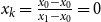
 ${x_k} = \left( {x - {x_0}} \right)/\left( {{x_1} - {x_0}} \right)$
for a predetermined age interval
 $\left[ {{x_0},{x_1}} \right]$
and
 ${x_k} \in \left[ {0,1} \right]$
. There are four coefficients
 $\alpha $
,
 $\omega $
,
 ${s_0}$
and
 ${s_1}$
for the Hermite basis functionsFootnote 2
 ${h_{ij}}\!\left( {{x_k}} \right),\;i = 0,1,\;j = 0,1$
to be estimated. Thereinto,
 $\alpha $
and
 $\omega $
correspond to
 ${p_0}$
and
 ${p_1}$
in (1) and reflect the level of
 $\ln {m_x}$
at the two boundary ages
 ${x_0}$
and
 ${x_1}$
, respectivelyFootnote 3.
We denote respectively
 $\boldsymbol{D}$
,
 $\boldsymbol{E}$
and
 $\boldsymbol{M}$
as the
 $\left( {{n_a} \times {n_y}} \right)$
matrices of the death counts, central exposures and central death rates sorted by age and year, where the total number of ages (years) equals
 ${n_a}$
(
 ${n_y}$
). It is assumed that the number of deaths is a random variable following a Poisson distribution. Suppose
 $\boldsymbol{d}$
,
 $\boldsymbol{e}$
and
 $\boldsymbol{m}$
are the vectors with a length of
 ${n_a}$
in the above matrices corresponding to a given year. In a matrix form, one may write the HS model as
 \begin{align}ln\ \boldsymbol{m} = {\boldsymbol{x}_{\textbf{0}}}{\boldsymbol\beta} ,\end{align}
where
 $\boldsymbol{m}$
is a vector of
 $\ln {m_x}$
with a length of
 ${n_a} = {x_1} - {x_0} + 1$
,
 ${\boldsymbol{x}_{\textbf{0}}}$
refers to a (
 ${n_a} \times 4$
) matrix containing the four Hermite basis functions at each age,
 $\boldsymbol{\beta} = \left( {\alpha ,\omega ,{s_0},{s_1}} \right)^{\prime}$
is the coefficient vector.
A smooth path between the youngest and oldest death rates in the interval is specified by
 ${s_0}$
and
 ${s_1}$
which give the gradients at the two boundary ages. As discussed in the original paper of the HS method, the fitted mortality curve may be too flexible and may deviate from the typical shape when both slope parameters are employed. Accordingly, four versions of the HS model can be constructed by setting one or both gradient coefficients to zero. The four models, namely HS1 (
 ${s_0} = {s_1} = 0$
), HS2 (
 ${s_1} = 0$
), HS3 (
 ${s_0} = 0$
) and HS4 can be defined by adjusting the coefficient vector
 $\boldsymbol\beta $
:
 \begin{align*}\boldsymbol\beta^{\prime} = \left\{ {\begin{array}{*{20}{c}}{HS1:\left( {\alpha ,\omega ,0,\;0} \right)}\\[3pt]{HS2:\left( {\alpha ,\omega ,{s_0},0} \right)}\\[3pt]{HS3:\left( {\alpha ,\omega ,0,{s_1}} \right)}\\[3pt]{HS4:\left( {\alpha ,\omega ,{s_0},{s_1}} \right)}\end{array}} \right..\end{align*}
As explained in section 1, the classical Gompertz law requires two parameters to model the decreasing mortality differentials over age and can potentially cause an unjustified crossover at advanced ages. On the other hand, the four HS models can ensure the convergence using only the parameter
 $\alpha $
. In the work of Richards (Reference Richards2020), the initial mortality level
 ${\alpha ^{\left( i \right)}}$
for population
 $i$
can be expressed as:
 \begin{align}{\alpha ^{\left( i \right)}} = {\alpha ^{\left( 0 \right)}} + \mathop \sum \nolimits_{j = 1}^J {\alpha ^{\left( {{r_j}} \right)}}{z^{\left( {i,j} \right)}},\end{align}
where
 ${z^{\left( {i,j} \right)}}$
is an indicator variable which equals 1 if population
 $i$
has risk factor
 $j$
(
 $j = 1,2, \ldots ,J$
) and 0 otherwise. When a population does not exhibit any of the
 $J$
risk characteristics, the intercept of the fitted mortality curve is equivalent to the baseline value
 ${\alpha ^{\left( 0 \right)}}$
. The estimated mortality level at the starting age increases by
 ${\alpha ^{\left( {{r_j}} \right)}}$
for each additional risk factor j. By way of illustration, suppose that mortality data with the same gender of two states in the same country only differ in one risk factor – state. Under the simplest model HS1, their mortality differentials can be incorporated using the individual starting values
 ${\alpha ^{(1)}} = {\alpha ^{\left( 0 \right)}}$
and
 ${\alpha ^{(2)}} = {\alpha ^{\left( 0 \right)}} + {\alpha ^{\left( {{r_1}} \right)}}$
and a common ending value
 $\omega $
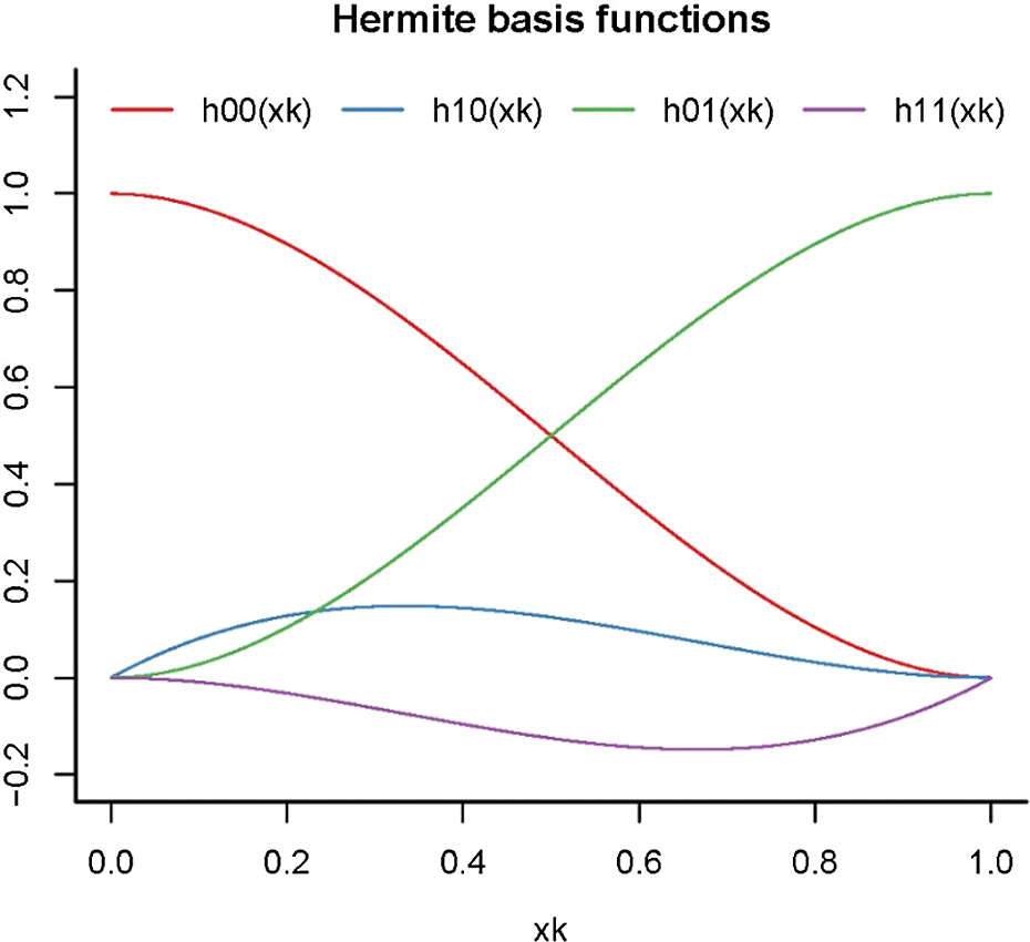
. Under the compensation law of mortality, the two sets of state-level mortality rates (in a specific year) should converge gradually as age increases. As shown in Figure 1 that plots the basis functions of HSs,
 ${h_{00}}\!\left( {{x_k}} \right)$
is monotonically decreasing over the defined age range. Consequently, the gap between the fitted mortality curves of the two populations vanishes over age by default, without the need of adopting a “slope” parameter.
Hermite basis splines
 ${h_{ij}}\!\left( {{x_k}} \right)$
for
 ${x_k}$
ranging from 0 to 1,
 $i = 0,1$
and
 $j = 0,1$
.
In addition to the parsimonious modelling of mortality differentials, the potential crossover problem under the Gompertz model can be avoided due to the monotonicity of the Hermite function
 ${h_{00}}\!\left( {{x_k}} \right)$
. Specifically, the difference between the log central death rates of the two populations at age
 $x$
under the HS1 model is calculated as
 \begin{align}ln\ m_x^{(1)} - ln\ m_x^{(2)} & = \left[ {{\alpha ^{(1)}}{h_{00}}\!\left( {{x_k}} \right) + \omega {h_{01}}\!\left( {{x_k}} \right)} \right] - \left[ {{\alpha ^{(2)}}{h_{00}}\!\left( {{x_k}} \right) + \omega {h_{01}}\!\left( {{x_k}} \right)} \right]\nonumber\\[3pt]& = \left( {{\alpha ^{(1)}} - {\alpha ^{(2)}}} \right){h_{00}}\!\left( {{x_k}} \right), \end{align}
where
 ${x_k} = \left( {x - {x_0}} \right)/\left( {{x_1} - {x_0}} \right)$
. Note that the two populations are assumed to share a common death rate
 $\ln {m_{{x_1}}} = \omega $
at an advanced age
 ${x_1}$
Footnote 4. Since
 ${h_{00}}\!\left( {{x_k}} \right)$
is a decreasing function ranging between 0 and 1, the difference in equation (6) narrows down to 0 as
 $x$
reaches
 ${x_1}$
but never switches its sign over the given range
 $\left[ {{x_0},{x_1}} \right]$
. Nonetheless, one may argue that mortality differentials resulted from certain risk factors such as gender reduce at higher ages but do not vanish entirely (Tickle, Reference Tickle1997). That is, one population always has lower death rates than the other for the entire age range considered
 $\big($
assuming
 ${\alpha ^{(1)}} \gt {\alpha ^{(2)}}$
and
 $\left.{\omega ^{(1)}} \gt {\omega ^{(2)}}\right)$
. To arrive at this pattern, a population-specific ending value
 ${\omega ^{\left( i \right)}}$
may be employed, producing mortality differentials as follows:
 \begin{align}ln\ m_x^{(1)} - ln\ m_x^{(2)} & = \left[ {{\alpha ^{(1)}}{h_{00}}\!\left( {{x_k}} \right) + {\omega ^{(1)}}{h_{01}}\!\left( {{x_k}} \right)} \right] - \left[ {{\alpha ^{(2)}}{h_{00}}\!\left( {{x_k}} \right) + {\omega ^{(2)}}{h_{01}}\!\left( {{x_k}} \right)} \right]\nonumber\\[3pt]& = \left( {{\alpha ^{(1)}} - {\alpha ^{(2)}}} \right){h_{00}}\!\left( {{x_k}} \right) + \left( {{\omega ^{(1)}} - {\omega ^{(2)}}} \right){h_{01}}\!\left( {{x_k}} \right).\end{align}
As illustrated in Figure 1,
 ${h_{00}}\!\left( {{x_k}} \right)$
is monotonically decreasing, while
 ${h_{01}}\!\left( {{x_k}} \right)$
is an increasing function. Besides, they are symmetric about the line
 $h\!\left( {{x_k}} \right) = 0.5$
 $\left({h_{00}}\!\left( {{x_k}} \right) + {h_{01}}\!\left( {{x_k}} \right) = 1\right)$
. It implies that when
 $\;\left( {{\alpha ^{(1)}} - {\alpha ^{(2)}}} \right) = \left( {{\omega ^{(1)}} - {\omega ^{(2)}}} \right)$
, the sum of the two weighted functions in (7) becomes a horizontal line. Since
 $\left( {{\alpha ^{(1)}} - {\alpha ^{(2)}}} \right)$
and
 $\left( {{\omega ^{(1)}} - {\omega ^{(2)}}} \right)$
refer to the differences in the log mortality rates between the two populations at the youngest and oldest ages, respectively, one would expect the former to be more pronounced than the latter due to the compensation law of mortality (Gavrilov & Gavrilova, Reference Gavrilov and Gavrilova2001). Accordingly,
 ${h_{00}}\!\left( {{x_k}} \right)$
contributes more to the weighted sum in equation (7), leading to declining but non-zero differentials. Again, the no-crossover property can be guaranteed, as the weighted sum of the two Hermite basis functions does not change in sign over the domain interval. The other three HS models also possess this property if one sets common gradient parameters
 ${s_0}$
and
 ${s_1}$
between related populationsFootnote 5.
The above HS models were initially proposed to model mortality over the age range rather than over time. Next, we show that the HS approach can be extended to model two-dimensional population mortality data. Similar to the widely adopted CBD model, the HS structure is fitted to the mortality data of each year. By doing so, the estimated values of each model parameter over different years form a time series, based on which the future death rates can be projected or simulated. The modified versions of the HS models are given below:
 \begin{align}ln\ \boldsymbol{M} = \boldsymbol{XB} = \left( {{\boldsymbol{I}_{{\boldsymbol{n}_{\boldsymbol{y}}}}} \otimes {\boldsymbol{X}_{\textbf{0}}}} \right)\boldsymbol{B},\end{align}
where
 $\boldsymbol{I}_{{\boldsymbol{n}_{\boldsymbol{y}}}}$
is an identity matrix of size
 ${n_y}$
,
 ${\boldsymbol{x}_{\textbf{0}}}$
has a dimension of
 $\left( {{n_a} \times 4} \right)$
and comprises the Hermite basis functions at each age, the design matrix
 $\boldsymbol{x}$
is the Kronecker product of
 $\boldsymbol{I}_{{\boldsymbol{n}_{\boldsymbol{y}}}}$
and
 ${\boldsymbol{x}_{\textbf{0}}}$
, the coefficient vector
 ${\textbf{B}} = \left( {\boldsymbol\beta^{\prime}_{\boldsymbol{t}_{\textbf{0}}},\boldsymbol\beta^{\prime}_{{\boldsymbol{t}_{\textbf{0}}} + \textbf{1}}, \ldots , \boldsymbol\beta^{\prime}_{{\boldsymbol{t}_{\textbf{1}}}}} \right)^{\prime}$
concatenates the year-specific HS coefficients
 ${\boldsymbol\beta _\boldsymbol{t}}$
. Again, the four HS versions can be obtained by adjusting
 ${\boldsymbol\beta _\boldsymbol{t}}$
. The modified versions of the HS models are given below:
 \begin{align*}\left\{ {\begin{array}{l}{HS1:\;\;\;ln\ {m_{x,t}} = {\alpha _t}{h_{00}}\!\left( {{x_k}} \right) + {\omega _t}{h_{01}}\!\left( {{x_k}} \right)}\\[4pt]{HS2:\;\;\;ln\ {m_{x,t}} = {\alpha _t}{h_{00}}\!\left( {{x_k}} \right) + {\omega _t}{h_{01}}\!\left( {{x_k}} \right) + {s_{0,t}}{h_{10}}\!\left( {{x_k}} \right)}\\[4pt]{HS3:\;\;\;ln\ {m_{x,t}} = {\alpha _t}{h_{00}}\!\left( {{x_k}} \right) + {\omega _t}{h_{01}}\!\left( {{x_k}} \right)\;\;\;\;\;\;\;\;\;\;\;\;\;\;\;\;\;\;\;\;\;\;\;\;\;\; + {s_{1,t}}{h_{11}}\!\left( {{x_k}} \right)}\\[4pt]{HS4:\;\;\;ln\ {m_{x,t}} = {\alpha _t}{h_{00}}\!\left( {{x_k}} \right) + {\omega _t}{h_{01}}\!\left( {{x_k}} \right) + {s_{0,t}}{h_{10}}\!\left( {{x_k}} \right) + {s_{1,t}}{h_{11}}\!\left( {{x_k}} \right)}\end{array}} \right..\end{align*}
Similar to the one-dimensional case,
 ${\alpha _t}$
and
 ${\omega _t}$
can be interpreted as the fitted values of
 $\ln {m_{{x_0},t}}$
and
 $\ln {m_{{x_1},t}}$
. The other two parameters
 ${s_{0,t}}$
and
 ${s_{1,t}}$
specify the smoothed pathway between the two mortality rates at the two boundary ages in year
 $t$
.
When the time dimension is included in modelling mortality data, avoiding any mortality crossover between related populations is not straightforward. Particularly, when the sample period covers more distant years, the observed mortality rates at the oldest ages are more volatile, and the data themselves may exhibit some crossover. Such features would not be helpful in determining the fitted mortality surface. We propose one possible solution to cope with this issue by imposing constraints on the second-level parameter
 ${\omega _t}$
. Consider males (population 1) and females (population 2) in the same country, when the two populations are assumed to share (only) the common gradient parameters
 ${s_{0,t}}$
and
 ${s_{1,t}}$
, for year t, the initial mortality differential
 $\left( {\alpha _t^{(1)} - \alpha _t^{(2)}} \right)$
should decrease to
 $\left( {\omega _t^{(1)} - \omega _t^{(2)}} \right)$
without changing its sign over the age range considered. This property is true if
 $\left( {\alpha _t^{(1)} - \alpha _t^{(2)}} \right)\left( {\omega _t^{(1)} - \omega _t^{(2)}} \right) \gt 0$
. Given
 $\alpha _t^{(1)} \gt \alpha _t^{(2)}$
for all
 $t$
,
 $\omega _t^{(1)} \gt \omega _t^{(2)}$
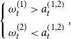
is required to avoid the potential crossover. In other words, the female population with lower mortality rates at the starting age is expected to maintain this “advantage” at the ending age. As we will discuss in more detail later, the maximum likelihood estimation with the Newton–Raphson iterative scheme is used to calibrate the model parameters. Nevertheless, the inequality constraints are not guaranteed to be satisfied during the estimation procedure. Accordingly, we adopt the barrier method (Wright & Nocedal, Reference Wright and Nocedal1999) under which the inequality constraints are incorporated using the so-called barrier functions that serve as a penalty term. It has been applied in mortality modelling by Li & Liu (Reference Li and Liu2020, Reference Li and Liu2021) to constrain their heat wave model parameters. As the parameter estimates approach the inequality bounds, the magnitude of the barrier functions rises to infinity, and so the log-likelihood is penalised more by such estimates. Then the optimised parameters are “forced” to fall within the boundaries.
For ease of exposition, consider an optimisation problem searching for parameter values that maximise a function
 $f\!\left( \theta \right)$
, subject to the constraint
 $\theta \gt a$
. Under the barrier method, the optimisation problem is redesigned as maximising the penalised function
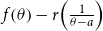 $f\!\left( \theta \right) - r\!\left( {\frac{1}{{\theta - a}}} \right)$
, where
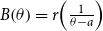 $B\!\left( \theta \right) = r\!\left( {\frac{1}{{\theta - a}}} \right)$
refers to the barrier function with
 $r \gt 0$
. Given a feasible initial value that over-satisfies the constraint, as
 $\theta $
decreases to its lower bound
 $a$
, the barrier function tends to infinity, which then contradicts the aim of maximisation. Accordingly, this formulation would avoid the violation of the parameter restriction. Similarly, the barrier functions for the constraints
 $\theta \lt b$
and
 $a \lt \theta \lt b$
can be constructed as
 $r\!\left( {\frac{1}{{b - \theta }}} \right)$
and
 $r\!\left( {\frac{1}{{b - \theta }} + \frac{1}{{\theta - a}}} \right)$
, respectively.
Setting the objective function to the Poisson log-likelihood function, multiple barrier functions can be embedded to manage the inequality constraints imposed on the population-specific
 $\omega _t^{\left( i \right)}$
. For example, when the male and female populations in the same country are considered, the following constraints are imposed:
 \begin{align*}\left\{ {\begin{array}{*{20}{c}}{\omega _t^{(1)} \gt a_t^{\left( {1,2} \right)}}\\[6pt]{\omega _t^{(2)} \lt a_t^{\left( {1,2} \right)}}\end{array}} \right.\!,\end{align*}
where
 $\omega _t^{(1)}$
and
 $\omega _t^{(2)}$
are the male and female level parameters at the ending age, respectively,
 $a_t^{\left( {1,2} \right)}$
is calculated as the average of the initial values of
 $\omega _t^{(1)}$
and
 $\omega _t^{(2)}$
. Under the careful design of the barrier method, the no-crossover condition
 $\omega _t^{(1)} \gt \omega _t^{(2)}$
can be met. The specifications of the barrier functions, initial values, penalised log-likelihood function and the updating equations for the HS4 model are provided in Appendix A. As we will show in section 3.2, the above barrier constraints can be applied similarly to risk factors other than gender.
2.2 Gompertz model
Gompertz (Reference Gompertz1825) discovered that the age-specific hazard rate of adult mortality increases exponentially with age and proposed a two-parameter model
 \begin{align*}{\mu _x} = B{c^x}\end{align*}
or equivalently
 \begin{align}ln\ {\mu _x} = {k_1} + {k_2}x.\end{align}
Since this discovery, actuaries and researchers have developed various modifications to the original designFootnote 6. For instance, Makeham (Reference Makeham1867) added an age-independent term to the above model for the age-specific hazard to account for deaths that do not result from senescence. Besides including more parameters, adjustments were made to the format of the original function. The so-called Perks model (Perks, Reference Perks1932) with four parameters adopted a logistic function, which is described as follows:
 \begin{align*}{\mu _x} = \frac{{A + B{c^x}}}{{1 + D{c^x}}}.\end{align*}
The well-known CBD model (Cairns et al., Reference Cairns, Blake and Dowd2006) can be obtained by replacing the hazard rate with the death rate and setting
 $A = 0$
and
 $B = D$
under the Perks law and adding a time dimension. Specifically, the probability of death
 ${q_{x,t}}$
is modelled as:
 \begin{align*}{q_{x,t}} = \frac{{{e^{{k_{1,t}} + {k_{2,t}}x}}}}{{1 + {e^{{k_{1,t}} + {k_{2,t}}x}}}}\end{align*}
or equivalently
 \begin{align*}logit\;{q_{x,t}} = ln \left( {\frac{{{q_{x,t}}}}{{1 - {q_{x,t}}}}} \right) = {k_{1,t}} + {k_{2,t}}x.\end{align*}
It is evident that the CBD model can be regarded as an application of the Gompertz law (equation (9)) applied to a transformed measure, in modelling population mortality data with both the age and time dimensions. This model has been widely applied and extended in the literature and has been found particularly suitable for explaining mortality rates at higher ages (Cairns et al., Reference Cairns, Blake, Dowd, Coughlan, Epstein, Ong and Balevich2009).
For comparison purposes, we utilise the logarithm of the central death rate rather than the logit probability of death for the two-dimensional Gompertz law in this paper. The log central death rate
 $\ln {m_{x,t}}$
of a life aged
 $x$
in year
 $t$
is expressed as
 \begin{align}ln\ {m_{x,t}} = {k_{1,t}} + {k_{2,t}}x,\end{align}
where
 ${k_{1,t}}$
refers to the level of the mortality curve in year
 $t$
and
 ${k_{2,t}}$
describes the speed at which mortality increases for each extra year of age in year t. The fitted log central death rates in a given year are assumed to grow linearly with age.
2.3 PS model
The two mortality models introduced above make assumptions about the functional form of mortality rates and only impose smoothness across adjacent ages. However, some academics are sceptical about specifying the mortality surface using defined functions. To address this concern, one branch of mortality models originated from the spline fitting technique that smooths mortality rates only based on features of data and avoids the identification of the model structure.
One of the most commonly applied methods in the actuarial literature is the PS model (Currie et al., Reference Currie, Durban and Eilers2004). The concept of PS was initially proposed by Eilers & Marx (Reference Eilers and Marx1996). They applied difference penalties on the coefficients of B-splines to strike a balance between the goodness of fit and smoothness of the fitted curve. This one-dimensional spline fitting approach was extended to a bivariate regression model in Eilers & Marx (Reference Eilers and Marx2003) and Eilers et al. (Reference Eilers, Currie and Durbán2006). Using the same notation as in section 2.1,
 $\boldsymbol{D}$
,
 $\boldsymbol{E}$
and
 $\boldsymbol{M}$
represent the matrices of the death counts, central exposures and central death rates, and
 $\boldsymbol{d}$
,
 $\boldsymbol{e}$
and
 $\boldsymbol{m}$
are the vector components corresponding to a given year
 $t$
.
The log death counts in year
 $t$
can be modelled as:
 \begin{align}ln\ \boldsymbol{d} = ln\ \boldsymbol{e} + ln\ \boldsymbol{m} = ln\ \boldsymbol{e} + \boldsymbol{Ba},\end{align}
where
 $\boldsymbol{B}$
is the
 $\left( {{n_a} \times k} \right)$
B-spline regression matrix containing polynomials connected at equally spaced knots, and
 $\boldsymbol{a}$
is the
 $\left( {k \times 1} \right)$
coefficient vector. The column dimension
 $k$
of
 $\boldsymbol{B}$
is equivalent to the sum of the polynomial degree
 $q$
and the number of (internal) knots
 ${n_{{d_x}}}$
(i.e.,
 $k = q + {n_{{d_x}}}$
). The more knots the regression employs, the more flexible the fitted curve is. One may adopt a sufficient number of knots for B-splines to provide more flexibility than needed and avoid over-fitting by constructing a difference penalty term that imposes smoothness (Eilers & Marx, Reference Eilers and Marx2002). Accordingly, the coefficient vector
 $a$
can be estimated by maximising the penalised log-likelihood
 \begin{align*}{l_p} = l\!\left( {\boldsymbol{a};\, \boldsymbol{d}} \right) - \frac{1}{2}\boldsymbol{a}^{\prime}\boldsymbol{Pa}, \end{align*}
where
 $l\!\left( {\boldsymbol{a};\,\boldsymbol{d}} \right)$
refers to the log-likelihood of Poisson distribution and the penalty matrix
 $\boldsymbol{P} = \lambda {\boldsymbol{\Delta }}^{\prime}{\boldsymbol{\Delta }}$
is composed of the smoothing parameter
 $\lambda $
and difference matrix
 ${\boldsymbol{\Delta }}$
with order 2.
The PS approach can also be applied to fitting the mortality surface across ages and years. We denote the
 $\left( {{n_a} \times {k_a}} \right)$
and
 $\left( {{n_y} \times {k_y}} \right)$
B-spline basis matrices associated with age
 $x$
and year
 $t$
by
 ${\boldsymbol{B}_a}$
and
 ${\boldsymbol{B}_y}$
, respectively. The number of equally spaced knots can be determined separately for the age and year horizons based on the data range. Then the B-spline matrix in the two-dimensional setting is constructed as the Kronecker product
 \begin{align*}{\boldsymbol{B}^{(\textbf{2})}} = {\boldsymbol{B}_y} \otimes {\boldsymbol{B}_a}.\end{align*}
Given mortality data across both ages and years, the PS model is expressed as:
 \begin{align}ln\ \boldsymbol{D} = \ln \boldsymbol{E} + \ln \boldsymbol{M} = \ln \boldsymbol{E} + \boldsymbol{B}^{(2)} \boldsymbol{a} = \ln \boldsymbol{E} + {\boldsymbol{B}_a} \boldsymbol{AB}^{\prime}_y,\end{align}
where
 $\boldsymbol{A}$
is the
 $\left( {{k_a} \times {k_y}} \right)$
matrix obtained by rearranging the coefficient vector
 $\boldsymbol{a}$
with a length of
 ${k_a}{k_y}$
. The parameters in the PS model are estimated by maximising the same Poisson log-likelihood function using a smoothing matrix that penalises the two dimensions of
 $\boldsymbol{A}$
separately. The penalty matrix is given as
 \begin{align*}\boldsymbol{P} = {\lambda _a}\!\left( {{\boldsymbol{I}_{{k_y}}} \otimes \boldsymbol\Delta^{\prime}_a{\boldsymbol\Delta _a}} \right) + {\lambda _y}\!\left( {\boldsymbol\Delta^{\prime}_y{\boldsymbol\Delta _y} \otimes {\boldsymbol{I}_{{k_a}}}} \right),\end{align*}
where
 ${\boldsymbol{I}_{{k_y}}}$
(
 ${\boldsymbol{I}_{{k_a}}}$
),
 ${\lambda _a}$
(
 ${\lambda _y}$
) and
 ${\boldsymbol\Delta _a}$
(
 ${\boldsymbol\Delta _y}$
) are the identity matrix, smoothing parameter and difference matrix contributing to the columns (rows) of
 $\boldsymbol{A}$
.
We have briefly reviewed the theoretical background of the PS method, more technical details and improvements on the fitting algorithm can be found in Currie et al. (Reference Currie, Durban and Eilers2004, Reference Currie, Durban and Eilers2006) and Eilers et al. (Reference Eilers, Currie and Durbán2006).
3. Fitting
3.1 Single-population fitting
To fit the above three models, we collect population mortality data of Australia, England and Wales, France, Japan and the United States from the Human Mortality Database (HMD, 2021). Specifically, the death counts and exposure to risk of both genders from 1950 to 2018 over ages 56–95 are employed for this analysis. Following Brouhns et al. (Reference Brouhns, Denuit and Vermunt2002), we assume that the number of deaths is a random variable following a Poisson distribution with the mean equal to the expected number of deaths. This Poisson assumption enables a rigorous framework to estimate the model parameters by maximising the log-likelihood function
 \begin{align}l = ln\ L = \mathop \sum \limits_{x,t} \left( {{d_{x,t}}\ ln\ {{\hat d}_{x,t}} - {{\hat d}_{x,t}} - ln\! \left( {{d_{x,t}}!} \right)} \right),\;\end{align}
where
 ${d_{x,t}}$
represents the observed death counts. The fitted number of deaths
 ${{\hat d}_{x,t}}$
is calculated as the product of the observed exposures and fitted mortality rates
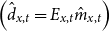 $\left({\hat d_{x,t}} = {E_{x,t}}{\hat m_{x,t}}\right)$
. As an illustration, the fitted death count for lives aged
 $x$
in year
 $t$
under the HS4 model is
 ${\hat d_{x,t}} = {E_{x,t}}{\hat m_{x,t}} = {E_{x,t}}\;{\rm{exp}}\!\left( {{\alpha _t}{h_{00}}\!\left( {{x_k}} \right) + {\omega _t}{h_{01}}\!\left( {{x_k}} \right) + {s_{0,t}}{h_{10}}\!\left( {{x_k}} \right) + {s_{1,t}}{h_{11}}\!\left( {{x_k}} \right)} \right)$
. For a parameter
 $\theta $
, the Newton–Raphson method is adopted to update its estimate iteratively as
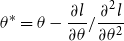 ${\theta ^*} = \theta - \dfrac{{\partial l}}{{\partial \theta }}/\dfrac{{{\partial ^2}l}}{{\partial {\theta ^2}}}$
. We provide below a summary of estimation steps under the HS4 model.
-
(1) Assign initial values to the parameters under the HS4 model and compute using the initial estimates. Specifically, we set
 ${\hat s_{0,t}} = {\hat s_{1,t}} = 0$
. The initial values of the other two parameters
${\alpha _t}$
and
${\omega _t}$
are set to the observed mortality levels at the two boundary ages
${x_0}$
and
${x_1}$
of the sample range in year
$t$
(i.e.,
${\hat \alpha _t} = \ln {m_{{x_0},t}}$
and
${\hat \omega _t} = \ln {m_{{x_1},t}}$
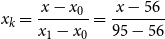
). For our sample,
${x_k} = \dfrac{{x - {x_0}}}{{{x_1} - {x_0}}} = \dfrac{{x - 56}}{{95 - 56}}$
.
-
(2) Update
${\alpha _t}$
as
$\hat \alpha _t^* = {\hat \alpha _t} + {\dfrac{\mathop \sum \nolimits_x \!\left( {{d_{x,t}} - {{\hat d}_{x,t}}} \right){h_{00}}\!\left( {{x_k}} \right)}{\mathop \sum \nolimits_x {{\hat d}_{x,t}}{{\left[ {{h_{00}}\!\left( {{x_k}} \right)} \right]}^2}}}$
. -
(3) Update
${\omega _t}$
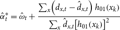
as
$\hat \alpha _t^* = {\hat \omega _t} + {\dfrac{\mathop \sum \nolimits_x \!\left( {{d_{x,t}} - {{\hat d}_{x,t}}} \right){h_{01}}\!\left( {{x_k}} \right)}{\mathop \sum \nolimits_x {{\hat d}_{x,t}}{{\left[ {{h_{01}}\!\left( {{x_k}} \right)} \right]}^2}}}$
. -
(4) Update
${s_{0,t}}$
as
$\hat s_{0,t}^* = {\hat s_{0,t}} + {\dfrac{\mathop \sum \nolimits_x \!\left( {{d_{x,t}} - {{\hat d}_{x,t}}} \right){h_{10}}\!\left( {{x_k}} \right)}{\mathop \sum \nolimits_x {{\hat d}_{x,t}}{{\left[ {{h_{10}}\!\left( {{x_k}} \right)} \right]}^2}}}$
. -
(5) Update
${s_{1,t}}$
as
$\hat s_{1,t}^* = {\hat s_{1,t}} + {\dfrac{\mathop \sum \nolimits_x \!\left( {{d_{x,t}} - {{\hat d}_{x,t}}} \right){h_{11}}\!\left( {{x_k}} \right)}{\mathop \sum \nolimits_x {{\hat d}_{x,t}}{{\left[ {{h_{11}}\!\left( {{x_k}} \right)} \right]}^2}}}$
. -
(6) Calculate the log-likelihood function
$l = \mathop \sum \nolimits_{x,t} \!\left( {_{x,t}\ln {{\hat d}_{x,t}} - {{\hat d}_{x,t}} - \ln \left( {{d_{x,t}}!} \right)} \right)$
using the parameters estimated in (2)–(5). -
(7) Repeat steps (2)–(6) until the improvement in
$l$
is small enough, e.g., the change in
$l$
between two iterations is less than
${10^{ - 7}}$
.





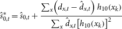

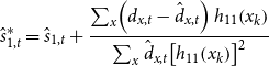



This study calibrates the HS and Gompertz models using the Poisson updating approach described above, while the PS model is fitted and forecasted using an R package “MortalitySmoothFootnote 7”. Both fitting methods are based on the Poisson maximum likelihood estimation, while the latter uses a so-called generalised linear array modelling that acts on matrices (Camarda, Reference Camarda2012). To examine the goodness of fit of the candidates, we calculate two measures – Akaike information criterion (AIC) and Bayesian information criterion (BIC) – as below:
 \begin{align*}AIC = - 2l + {n_p} \times 2\\[3pt]BIC = - 2l + {n_p}\ ln\ {n_d},\end{align*}
where
 $l$
refers to the Poisson log-likelihood function, and
 ${n_p}$
is the number of effective parameters. These two criteria penalise the likelihood by the number of parameters involved in the model with a penalty factor of 2 and the log of data counts (
 ${n_d}$
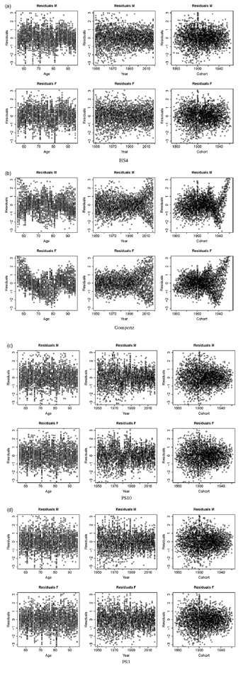
), respectively. The information criteria and residuals plots are provided in Table 1 and Figure 2, respectively.
Effective number of parameters (
 ${n_p}$
), log-likelihood values (
 $l$
), AIC and BIC values under the HS1-4, Gompertz, PS10 and PS3 models. The mortality models are ranked from 1 (the lowest AIC/BIC) to 6 (the highest AIC/BIC) and the ranks are given in brackets.

Some interesting remarks can be made from Table 1 that lists the model comparison criteria values for both genders of the ten datasets. Firstly, HS1-3 models always produce greater AICs and BICs than the full HS4 model. Note that
 ${\alpha _t}$
and
 ${\omega _t}$
are interpreted as the mortality rates at the two boundaries of the age interval. Essentially, the fitted mortality curves in each year under the HS1 model are assumed to have a shape determined by the two Hermite functions linking the starting and ending points. Such a specification may be too rigid for modelling population mortality data, which is vividly demonstrated by the worst performance of the HS1 model. Employing additional gradient factors can introduce more flexibility to the model and so can improve the goodness-of-fit, which can be seen from the better ranks of the HS2-4 models.
Comparing between the HS2 and HS3 models with one gradient factor
 ${s_{0,t}}$
and
 ${s_{1,t}}$
, respectively, the former only outperforms the latter for males in Australia and England and Wales. Since
 ${s_{0,t}}$
(
 ${s_{1,t}}$
) controls the pattern of the fitted mortality curves leaving from (approaching) the starting (ending) age, one may suspect that there have been more variations in the mortality development of older age groups. Under the full HS model, employing two gradient factors yields significantly better fitting performance than the other HS candidates. As a benchmark, the Gompertz model is specified by two time-varying components and gives smaller AIC and BIC values than the HS1-2 models in all cases. However, it consistently underperforms the HS4 model (and HS3 model in some cases).
Standardised deviance residuals plots under the HS4, Gompertz, PS10 and PS3 models for Australian males (top panel) and females (bottom panel).

The above five models all propose a functional form for mortality rates in the age dimension, while no smoothness assumption across periods is imposed. On the other hand, the PS approach produces a smoothed mortality surface using splines connected by knots. We consider the PS10 and PS3 models with a different number of knots. Specifically, the PS10 (PS3) refers to the PS model with one internal knot per 10 (3) data points in each dimension. The PS3 model tends to be the optimal choice among the seven candidates for males in four out of the five countries, while the HS4 model appears to be preferred for female populations. When fewer internal knots are adopted, the PS10 model tends to underperform the HS4 model but still performs better than the Gompertz model in all cases.
Figure 2 depicts the deviance residuals against age, period and cohort year for Australia. Only the HS4, Gompertz, PS10 and PS3 models, which have similar AIC/BIC values, are presented. It is apparent that the residuals are generally quite random under the HS4 and two PS models. However, those produced by the Gompertz method do exhibit obvious patterns, which may suggest the need for more parameters. Moreover, the residuals plotted against age under the four models (and the residuals against year under the PS models) show some “bars” at certain ages (in certain years). Since the HS4 and Gompertz models do not assume smoothed mortality rates in the period dimension, the time-varying parameters would capture the pattern in each year separately and lead to more scattered residuals against year. This difference is a direct consequence of different smoothness assumptions between the mortality models.
Based on these observations, one can see that imposing smoothness on both the age and time dimensions can lead to missing out some important patterns, though having the advantage of a smaller number of effective parameters. For those mortality models that only impose the smoothness assumption on the age dimension (HS and Gompertz models), more parameters are used to describe the temporal developments more adequately. It is noteworthy that an outstanding fitting performance does not guarantee accurate forecasting. As we will see later, the forecasting performance under the PS approach is subject to great uncertainty, though the fitting results are superior. Backtesting will be conducted and presented in section 5 to investigate the forecast accuracy of the mortality models.
3.2 No-crossover property of the HS models
As discussed in section 2.1, the key strength of the HS approach is that mortality crossover is avoided via the properties of Hermite basis functions. Mortality differentials due to risk factors other than gender decrease as age increases, portrayed by the level parameter
 ${\alpha _t}$
specifically for each population. When the gender effect is considered, mortality differentials diminish with increasing age but never vanish entirely. By imposing constraints on the level parameter specifically for each population
 $\left\{ {\begin{array}{*{20}{c}}{\omega _t^{(1)} \gt a_t^{\left( {1,2} \right)}}\\[6pt]{\omega _t^{(2)} \lt a_t^{\left( {1,2} \right)}}\end{array}} \right.\!,$
the HS models can capture such a feature even if there is occasional mortality crossover in the data. In contrast, the Gompertz and PS models are incapable of modelling this pattern.
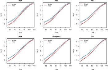
As an illustration of this crossover issue, we choose the mortality data for ages between 56 and 108Footnote 8 and years from 1950 to 2018. Figure 3 presents the observed and fitted log central death rates for the United States in 2018 under the six models. The PS approach here adopts one internal knot per 10 data points in each dimension to alleviate the potential crossover issue caused by overfitting. It can be seen that the HS1-3 models tend to underestimate the mortality rates at younger ages. The constructed shape of the HS1 and HS2 curves fits poorly at the oldest ages. On the other hand, the Gompertz model proposes a linear mortality curve of age and fails to capture the curvature observed at the highest ages. By comparison, the fitted curves under the HS4 and PS models follow the historical patterns more closely. However, the curves fitted under the PS model adhere to the data very closely, potentially indicating overfitting and lack of smoothness, even after applying the penalty structure. Another concern from Figure 3 is the intersection of the fitted female and male central death rates under the Gompertz and PS models at advanced ages. Under the compensation law of mortality, one would expect the gap between two genders to decline gradually over increasing age. But there is no biological basis to justify any crossover. Overall, the four HS models can generate a smoothed mortality curve that captures the relationships between males and females in the same country. Given appropriate constraints imposed on
 $\omega _t^{\left( i \right)}$
, the no-crossover property can be ensured.
Historical (dots) and fitted (solid lines) log central death rates in 2018 for the United States.

In addition to gender, the no-crossover property of the HS method holds when more risk factors are considered. As explained in equation (7) and footnote 6, when common gradient parameters are assumed for associated populations, the fitted mortality curves from the HS models would demonstrate narrowed gaps without an unreasonable crossover. This assumption should only be imposed if one believes that the populations under study exhibit similar paths of reaching the boundary mortality rates over the age interval. We have illustrated that the HS4 model tends to produce a good fit for mortality rates of males and females in the United States. Next, the fitting performances of the HS4, Gompertz and PS models are investigated when two risk factors – gender and country – are employed. Since the five countries considered in this study may not be highly related, the common-gradient assumption can be inappropriate. Accordingly, mortality data between 2008 and 2018 of females and males in Scotland and England and Wales are used for this particular illustrationFootnote 9. Based on the observations on
 $\alpha _t^{\left( i \right)}$
of the four populations, the following restriction is required for the HS4 model to avoid the potential crossover:
 \begin{align*}\omega _t^{\left( {m2} \right)} \gt \omega _t^{\left( {m1} \right)} \gt \omega _t^{\left( {f2} \right)} \gt \omega _t^{\left( {f1} \right)},\end{align*}
where
 $\omega _t^{\left( {m1} \right)}$
and
 $\omega _t^{\left( {f1} \right)}$
 $\left(\omega _t^{\left( {m2} \right)}\right.$
and
 $\left.\omega _t^{\left( {f2} \right)}\right)$
represent the level parameter of the female and male populations in England and Wales (Scotland). To conform with the constraint format of the barrier method, the above inequality can be converted into:
 \begin{align*}\left\{ {\begin{array}{*{20}{c}}{\omega _t^{\left( {m2} \right)} \gt a_t^{\left( {1,2} \right)}\;\;\;\;\;\;\;\;\;\;\;\;\;\;\;\;}\\[5pt]{a_t^{\left( {2,3} \right)} \lt \omega _t^{\left( {m1} \right)} \lt a_t^{\left( {1,2} \right)}}\\[5pt]{a_t^{\left( {3,4} \right)} \lt \omega _t^{\left( {f2} \right)} \lt a_t^{\left( {2,3} \right)}}\\[5pt]{\omega _t^{\left( {f1} \right)} \lt a_t^{\left( {3,4} \right)}\;\;\;\;\;\;\;\;\;\;\;\;\;\;\;\;}\end{array}} \right.\!,\end{align*}
where
 $a_t^{\left( {j,j + 1} \right)}$
is computed as the average of the
 ${j^{th}}$
and
 ${\left( {j + 1} \right)^{th}}\;\left( {j = 1,2,3} \right)$
highest initial values of the level parameter at the ending age. Note that other relationships among
 $\omega _t^{\left( i \right)}$
’s can be assumed. For example, if one believes that populations with the same gender will converge to the same level at the ending age (regardless of the country), a common
 $\omega _t^{\left( m \right)}$
 $\left(\omega _t^{\left( f \right)}\right)$
could be employed.
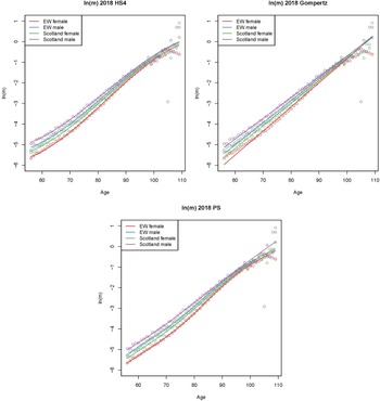
Figure 4 displays the observed and fitted mortality rates in 2018 under the three mortality models. The PS curves show unwarranted bends due to the lack of smoothness. Although the Gompertz model captures the decreasing mortality differentials over age, evident crossovers are observed at around age 100. Under the HS4 model, the fitted mortality differentials for populations with the same gender in the two countries (red and green curves, blue and purple curves) tend to reduce towards a small gap at advanced ages. For males and females in the same country, the differences in fitted mortality rates diminish with increasing age but never vanish entirely. To conclude, the HS4 model seems to strike a good balance between the goodness-of-fit and smoothness. More importantly, the HS4 model can describe the law of mortality properly and avoid the unjustified mortality crossover that presents under the Gompertz and PS models.
Fitted log central death rates in 2018 of females and males in Scotland and England and Wales.

4. Long-Term Prediction Performance
4.1 Time series models
This study now proceeds to examine the long-term performance of the six mortality models. The PS model extrapolates mortality rates not covered by the sample range during the fitting process by treating them as missing values. The R package “MortalitySmooth” offers the facility of both model estimation and projection, given a predetermined penalty order. In this study, we follow the suggestion by Currie et al. (Reference Currie, Durban and Eilers2004) and use the default penalty order of 2 for both the age and period dimensions, which implies that (log) mortality rates are predicted via (approximately) linear extrapolation. Under the HS and Gompertz models, the time-varying parameters are modelled by time series processes and projected to a future period to predict mortality levels. We first conduct a unit root test for each of the period factors
 ${\alpha _t}$
,
 ${\omega _t}$
,
 ${s_{0,t}}$
,
 ${s_{1,t}}$
,
 ${k_{1,t}}$
and
 ${k_{2,t}}$
.
The results suggest that all the period factors are not stationary at 5% significance level under the five models except for the female
 ${\omega _t}$
of Australia under the HS3 model, female
 ${\omega _t}$
of France under the HS4 model, female
 ${s_{1,t}}$
of Japan under the HS3 and HS4 models and male
 ${s_{0,t}}$
of Japan under the HS4 model. When using a 1% significance level, the unit root is detected for all the time series processes. We decide to fit the time-varying factors in the same mortality model by a multivariate (bivariate) random walk with drift (RWD):
 \begin{align}{\boldsymbol\theta _{\boldsymbol{t}}} = {\boldsymbol\theta _{\boldsymbol{t} - \textbf{1}}} + \boldsymbol\mu + {\boldsymbol{Z}_{\boldsymbol{t}}},\end{align}
where
 ${\boldsymbol\theta _{\boldsymbol{t}}}$
is a
 $\left( {n \times 1} \right)$
vector of the
 $n$
time-varying factors in a mortality model in year
 $t$
,
 $\boldsymbol\mu $
refers to the corresponding drift vector,
 ${\boldsymbol{Z}_{\boldsymbol{t}}}$
contains
 $n$
multivariate Gaussian error terms with mean zero. Although other time series choices can be considered, the RWD model has been widely adopted in the literature to extrapolate the decreasing trend of mortality (e.g., Cairns et al., Reference Cairns, Blake and Dowd2006; Dowd et al., Reference Dowd, Cairns, Blake, Coughlan, Epstein and Khalaf-Allah2010c). In addition, the assumed linear extrapolation under the multi-dimensional RWD process allows for a fair comparison between the PS approach with the second-order penalty and the other five models.
Estimated (solid lines) and projected (dashed lines) period factors in the HS1-4 and Gompertz models for males in England and Wales.

Figure 5 displays the estimated and projected parameters in the HS1-4 and GompertzFootnote 10 models for males in England and Wales. As illustrated, the two level parameters
 ${\alpha _t}$
and
 ${\omega _t}$
show a clear declining trend under the HS models, though the downward tendency in
 ${\omega _t}$
becomes less prominent under the HS3 model. This observation aligns with our expectations because these parameters are interpreted as the fitted mortality rates at the youngest and oldest ages of the sample which have been improving over time. Furthermore, the behaviour of
 ${s_{0,t}}$
and
 ${s_{1,t}}$
varies to some extent under different models. For example, the estimated
 ${s_{0,t}}$
values under the HS2 model (second row) demonstrate a generally decreasing trend over time. However, under the full model (fourth row), the declining tendency becomes less clear and more fluctuations can be found in the estimated
 ${s_{0,t}}$
values. Similarly, although the estimated
 ${s_{1,t}}$
values have been increasing since around 1980 under both the HS3 (third row) and HS4 (fourth row) models, the latter tends to show more fluctuating patterns. Besides, one may notice that the intercept and slope parameters
 ${k_{1,t}}$
and
 ${k_{2,t}}$
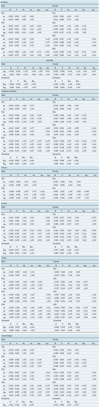
in the Gompertz model (first row) show an opposite trend to each other. It indicates that the average mortality level has been improving, and this reduction has been larger at the younger ages. Though not presented here, the parameter estimates exhibit similar trends for females and males in the five countries. Then we model the time-varying parameters as the multi-dimensional RWD. The estimated drift terms, standard deviations and correlation matrices are presented in Table B.1 in Appendix B.
4.2 Long-term projections
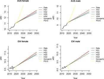
After obtaining the time series forecasts, future mortality rates can be calculated by updating the predicted time-varying components. It is of interest to investigate the impact of employing different model structures on mortality forecasts. We calculate life expectancies at key ages over the projection period. Since our data only cover ages up to 95, the Coale–Kisker approach (Coale & Kisker, Reference Coale and Kisker1990) is applied to extend the mortality rates to an “ultimate” age 110 with a presumed log central death rate of 0.7 (Gampe, Reference Gampe2010)Footnote 11. Figure 6 shows the Australia and England and Wales observed life expectancy at age 80 (
 ${e_{80}}$
), with projections up to the year 2050.
Observed and projected life expectancy at age 80 for Australia and England and Wales from 2010 to 2050. For demonstration purposes, the projections under the HS4 and Gompertz models are displayed in dashed lines.

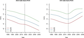
It is apparent that the PS10 model (yellow curves) predicts significantly longer life expectancy than the other model candidates for Australia. We remark that the projections produced under the PS10 model become particularly unreasonable when mortality data of England and Wales are employed – declining life expectancies over time. As demonstrated in Figure B.1 in Appendix B that plots the fitted and extrapolated mortality rates at ages 60, 70 and 80, the projected mortality rates for England and Wales exhibit an increasing tendency, which is not the case for Australia. The potential reason could be the slowing down of mortality improvement over the most recent few years in England and Wales. Since mortality rates are not predicted by selecting appropriate time series processes to ensure biological reasonableness, it is possible to observe unrealistic patterns in the forecasts under the PS approach.
The potentially unstable projections of the PS model were highlighted in previous studies. For example, based on Italian populations, Cocevar (Reference Cocevar2007) obtained insensible mortality forecasts for females, while the performance is reasonable for males. Richards et al. (Reference Richards, Ellam, Hubbard, Lu, Makin and Miller2007) examined the prediction performance of the two-dimensional PS method using mortality data of seven countries and found erratic forecasts in some cases. They argued that the PS method tends to balance irregular effects in data with smoothing and those features are carried through to projections.
We also investigate the long-term prediction performance under the PS model using different number of knots, while there is no optimal knot choice that can produce sensible forecasts for all datasets. In addition, though excessive knots are penalised to generate a reasonable effective dimension, they tend to yield even more volatile forecasts. Therefore, only the prediction performance of the PS10 model is presented in the remainder of the paper.
Besides this noticeable (and unreasonable) deviation under the PS method, there exist some differences among the other models. Firstly, the HS1 model that obtains future mortality rates by projecting the mortality levels at the initial (56) and ending (95) ages results in the longest life expectancy of the four HS models. As depicted in Figure 6, adding one or two gradient parameters tends to reduce the predicted values. For example, the green curves under the HS3 model almost always lie below the other four sets of predictions (excluding the PS method) for the two ages. This can be attributed primarily to the less linear trend of the second level parameter
 ${\omega _t}$
. For example, it can be seen from Figure 5 that the projected values of
 ${\hat{\omega} _t}$
(the projected
 $ln\ {\widehat{m}}_{x_{1},t}$
) from the HS3 model are generally higher than those from the other HS candidates, while the HS3
 $ {\widehat{\alpha}}_{t}$
(the projected
 $ln\ {\widehat{m}}_{x_{0},t}$
) values are similar to those from the HS2 model. One would expect the former to predict longer life expectancy than the latter. Although not presented here, for all the datasets the projections under the HS2 (blue) and HS4 (purple) models tend to lie within the two boundary curves formed by the other two HS candidates for all the datasets. Gompertz projections tend to be similar to those for HS1, with differences of less than 0.1–0.2 years in 2050.
Overall, the HS1-4 and Gompertz models give sensible forecasts of life expectancies. The PS model predicts unreasonably high or decreasing life expectancies, possibly caused by the automatic extrapolation process that may have overfitted the data and misused the random noises therein.
5. Backtesting
In the above analysis, we notice some similarities and discrepancies among the mortality forecasts under the six models. This section investigates the accuracy of their predictions via backtesting (also known as out-of-sample testing). In more detail, the sample period is split into two parts for calibrating the model parameters and testing the forecasting performance, respectively. Since the actual mortality rates are given over the testing period, the forecast accuracy of each model can be assessed by comparing the projected values against the observations. We adopt the root mean squared error (RMSE) to examine the forecasting performance quantitatively. To attain a better insight into the capability of generating sensible forecasts, the comparison is made across age, time and both dimensions using the following three measures:
 \begin{align}RMS{E_x} & = \sqrt {\dfrac{1}{N}\mathop \sum \limits_{h = 1}^N {{\left( {ln\ {m_{x,T + h}} - ln\ {{\hat m}_{x,T + h}}} \right)}^2}} \nonumber\\[5pt]RMS{E_h} & = \sqrt {\dfrac{1}{{\left( {{x_1} - {x_0} + 1} \right)}}\mathop \sum \limits_{x = {x_0}}^{{x_1}} {{\left( {ln\ {m_{x,T + h}} - ln\ {{\hat m}_{x,T + h}}} \right)}^2}} \\[5pt]RMS{E_{all,h}} & = \sqrt {\dfrac{1}{{\left( {{x_1} - {x_0} + 1} \right) \times h}}\mathop \sum \limits_{j = 1}^h \mathop \sum \limits_{x = {x_0}}^{{x_1}} {{\left( {ln\ {m_{x,T + j}} - ln\ {{\hat m}_{x,T + j}}} \right)}^2}} ,\nonumber\end{align}
where
 $T$
is the ending year of the calibration period,
 $N$
is the total length of the testing period,
 ${x_0}$
(
 ${x_1}$
) corresponds to the minimum (maximum) value in the age interval and
 ${m_{x,T + h}}({\widehat{m}_{x,T + h}})$
represents the observed (predicted) central death rate.
 ${\rm{RMS}}{E_x}$
(
 ${\rm{RMS}}{E_h}$
) refers to the root mean squared error at age
 $x$
(in the
 ${h^{th}}$
year of forecasting) averaged across all projection years (ages), and
 ${\rm{RMS}}{E_{all,h}}$
gives a measure considering all ages and predictions up to year
 $T + h$
. The results of a 10-step forecasting horizon are provided in Figures 7–8 and Table 2.
 $RMS{E_{all,10}}$
(%) under the HS1-4, Gompertz and PS10 models. The mortality models are ranked from 1 (the lowest prediction error) to 6 (the highest prediction error) and the ranks are given in brackets.

 $RMS{E_x}$
values averaged over 10 forecasting steps.

 $RMS{E_h}$
values averaged across ages 56–95.

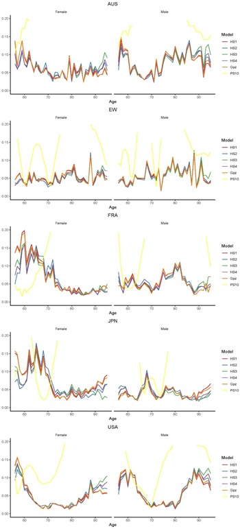
Figure 7 plots the 10-step
 ${\rm{RMS}}{E_x}$
under the six mortality models against age. Specifically, the prediction errors under the HS2 and HS4 models are somewhat similar for all the datasets. At the youngest and oldest ages, they deviate slightly, in which the HS2 errors are smaller than the HS4 errors. Over older ages, the HS3 model tends to produce the highest RMSE values among the HS candidates for four out of the five countries. Interestingly, the simplest model does not always lead to the lowest forecast accuracy. For example, the HS1 errors tend to be larger than the other HS errors at younger ages but performs better as age increases. One exception is Japan, for which the HS1 curves lie above the others at the oldest ages.
As a benchmark, the Gompertz model exhibits comparable results to the HS1 model. Comparing with the HS family, this baseline model tends to produce moderately more accurate mortality forecasts at advanced ages (greater than age 90), whereas its performance is less desirable at younger ages (before age 65). Unlike the above five models that generate similar
 ${\rm{RMS}}{{\rm{E}}_x}$
patterns across genders and countries, the performance of the PS10 model appears to be highly dependent on the dataset involved. When French and Japanese male data are employed, the PS approach seems to produce appealing forecast accuracy for certain age groups. Nevertheless, the RMSE values under the PS method are unusually high for the other datasets, casting doubt on the robustness of its forecasting performance.
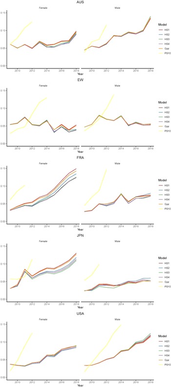
Averaging over all ages, one can compare the prediction errors under the six mortality models over time horizons. As depicted in Figure 8, the curves generally show an upward trend, indicating the increasing uncertainty in mortality forecasts in the more distant future. Based on the mortality data in Australia, England and Wales and France, the HS4 model appears to be the best performing candidate amongst the six, while HS3 and HS2 are preferred for Japan and the United States, respectively. The benchmark Gompertz method has a prediction performance similar to the HS1 model and is almost always worse than the HS2 and HS4 models. Again, the performance of the PS approach depends heavily on the dataset used to calibrate the parameters. Overall, it fails to reliably predict mortality rates for the five countries.
After examining the model performance in the age and time dimensions separately, we now move on to a two-dimensional measure
 $RMS{E_{all,h}}$
to make a more comprehensive assessment. The
 $RMS{E_{all,10}}$
values averaged over all ages and years for the five countries are tabulated in Table 2. For both genders, the HS4 model tends to be the best performing candidate for three out of the five datasets, and it also produces decent forecast accuracy for the other two countries. Interestingly, the parsimonious HS1 model that is not often preferred in the previous analysis produces the best forecast accuracy for males in the United States. The Gompertz approach ranks in the middle among the six mortality models. In line with the above findings, the PS model always has notably high prediction errors, which highlights the robustness issue of the forecasting performance of the PS model.
One may argue that the forecasting performances of the mortality models might vary significantly with the split between the calibration and testing periods. In order to examine the robustness of the backtesting results, we repeat the analysis using a 20-step forecasting horizon. For the sake of brevity, only the overall performance measure
 $RMS{E_{all,20}}$
is presented in Table 3. With a longer forecasting horizon, the HS2 model is preferred for females (males) in three (two) out of the five countries. The HS4 model gives the lowest prediction error for both genders in France and is mostly the second or third best method for the other datasets. In comparison, the other two HS members demonstrate more variations in the rank of the forecasting performances.
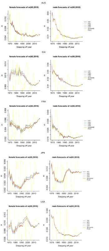
A sensible mortality model is expected to generate stable predictions. To further examine the forecast uncertainty of the six mortality models, a contracting horizon backtesting (Dowd et al., Reference Dowd, Cairns, Blake, Coughlan, Epstein and Khalaf-Allah2010c) is conducted. In more detail, we calibrate the mortality models on 20-year sequential subsamples and obtain mortality predictions for a pre-specified “future” year (year 2018). The first subsample covers data from 1950 to 1969, then from 1951 to 1970, and so on until the ending year (stepping-off year) of the fitting period reaches 2017. One would expect the predicted mortality rates on the forecast date to converge steadily to the observed values as the stepping-off year increases. Figure 9 visualises the forecasts in 2018 under the six models, using the mortality rates at age 65 as an example. All the mortality models except the PS approach illustrate similar paths of the projected central death rates. For most populations, the forecasts show a smooth curve that gradually converges towards the observed values, suggesting a stable progression of the model parameters between the sequential subsamples. As age increases (not presented here), the mortality data are more volatile, and the paths of forecasts tend to be less smooth. Nevertheless, the HS1-4 and Gompertz models still tend to share similar patterns. For the PS model, the paths fluctuate extensively and are not consistent with other methods, suggesting that the robustness of the prediction performance is a concern.
 $RMS{E_{all,20}}$
(%) under the HS1-4, Gompertz and PS10 models. The mortality models are ranked from 1 (the lowest prediction error) to 6 (the highest prediction error) and the ranks are given in brackets.

Forecasts of the central death rates in 2018. Mortality models are calibrated from 20-year sequential subsamples ending in the stepping-off year. The plus sign refers to the observed
 ${m_{65,2018}}$
.

Projected values (solid lines) and 95% prediction intervals (dashed lines) of survivor index
 $S\!\left( {65,t} \right)$
of the cohort aged 65 in 2009. The cross sign in the figure denotes the observed survivor index. The mortality models are calibrated on years 1950–2008 and projected/simulated over a 10-year forecasting horizon.

In summary, our out-of-sample testing indicates that the HS family, especially the HS4 model, tends to generate a comparable or higher degree of forecast accuracy than the benchmark Gompertz model. Furthermore, the unstable performance of the PS model suggests that extrapolating patterns without considering the temporal structure of mortality developments explicitly can give rise to unreasonable predictionsFootnote 12. The lack of robustness of the forecasting performance of the PS model is also addressed in Bohk-Ewald and Rau (Reference Bohk-Ewald and Rau2017) and Camarda (Reference Camarda2019).
6. Simulation study
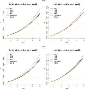
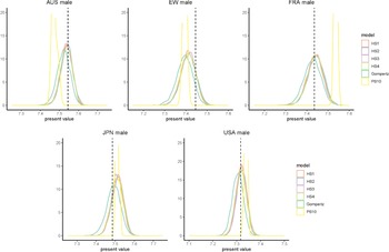
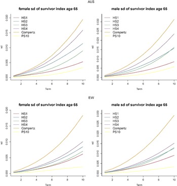
So far, we have investigated the predictive power of the six mortality models using backtesting and RMSE. Another crucial aspect of model examination lies in the level of uncertainty of the generated mortality scenarios. In practice, life insurance companies are required to prepare capital for mortality and longevity risk based on risk measures such as the 99.5% Value-at-Risk (VaR) and expected shortfall (conditional VaR). Therefore, the degree of variation in mortality simulations under a mortality model plays a vital role in pricing longevity-/mortality-linked products and preparing reserves. This section studies the performances of the candidate models using the semi-parametric bootstrap (Brouhns et al., Reference Brouhns, Denuit and Van Keilegom2005) that incorporates both the process error (uncertainty in time series processes for the HS and Gompertz models) and parameter error (uncertainty in parameter estimation for all the six models) into the analysis. Firstly, a pseudo sample of death counts is simulated from a Poisson distribution with the mean being the observed number of deaths. Then we fit the six mortality models to the pseudo sample and generate one set of future mortality scenarios. This process is repeated to generate 5,000 scenarios. Note that the PS model does not involve simulating future paths of time series processes, so the only source of uncertainty for the PS model is the parameter error. Following Cairns et al. (Reference Cairns, Blake, Dowd, Coughlan, Epstein, Ong and Balevich2009), the survivor index
 $S\!\left( {x,t} \right) = \mathop \prod \nolimits_{i = 0}^t \!\left( {1 - {q_{x + i,T + i}}} \right)$
representing the probability that the cohort aged
 $x$
in year
 $T$
survives to year
 $T + t$
is employed to compare the model performance, where
 ${q_{x,T}}$
is the probability that a life aged
 $x$
in year
 $T$
will die in one year. Using a 10-year testing period, we plot in Figure 10 the projected
 $S\!\left( {65,t} \right)$
for the cohort aged 65 in the first prediction year. For illustration purposes, only the 95% prediction intervals of the HS4, Gompertz and PS models are presented.
For the ten datasets, the predicted survivor indices under the HS1-4 and Gompertz models follow roughly the same path as the observed values (cross signs). But when the PS model (yellow) is applied, there exists an obvious overestimation (underestimation) of the death rates for France and females in the United States (Australia). Besides, the simulated mortality distribution from the PS model only incorporates the parameter uncertainty, so its prediction intervals tend to be narrower than the others. Under the Gompertz model, the 95% prediction intervals are slightly broader than those under the other four HS candidates. Within the HS family, the prediction bounds are rather close to one another, though the full model appears to generate the widest prediction bounds because it involves more time series processes and potentially greater process error. All the mortality models except the PS model can produce prediction intervals that capture the observed values (the prediction intervals under the HS1-3 models are not displayed).
A more pronounced reflection is illustrated in Figure 11 that displays the standard deviations of
 $S\!\left( {65,t} \right)$
. At the end of the testing period (
 $t = 10$
), the Gompertz model demonstrates the greatest variations, followed by the HS candidates and the PS model. As discussed above, the HS4 model tends to create more variations in the simulated scenarios of
 $S\!\left( {65,t} \right)$
. However, the differences in the standard deviations of
 $S\!\left( {65,t} \right)$
within the HS family are not significant, and no general conclusion can be made on their ordinal relationship.
Standard deviation of survivor index
 $S\!\left( {65,t} \right)$
of the cohort aged 65 in 2009,
 $t = 1,2, \ldots ,10$
. The mortality models are calibrated on mortality data in Australia and England and Wales over 1950–2008 and projected/simulated over a 10-year forecasting horizon. Multivariate RWD is fitted to the time-varying parameters.

The above results for the HS1-4 and Gompertz models are based on the multivariate RWD model. If the time-varying parameters are modelled separately by univariate RWD processes regardless of the strong correlation, the level of process uncertainty may differ significantly. We then investigate the impact of the correlation structure of the time series models on the prediction intervals. Since the projection results are not affected under this independence setting, we only present the standard deviations of
 $S\!\left( {65,t} \right)$
for the same populations in Figure B.2 in Appendix B. At the end of the testing period (
 $t = 10$
), the Gompertz model demonstrates the greatest variations, followed roughly by the HS4, HS2, HS3 and HS1 models. Although the estimated standard errors of the time series models for the Gompertz parameters have a similar magnitude to those for the HS parameters, the time-varying parameters in these two types of models are scaled differently. Under the Gompertz model,
 ${k_{1,t}}$
and
 ${k_{2,t}}$
are multiplied by 1 and
 $x$
(from 56-95), respectively. On the other hand, the HS parameters are scaled by the Hermite basis functions that are less than 1 in magnitude. Without considering the correlation structure, the 95% prediction intervals under the Gompertz model would be much broader than those under the other four HS candidates. Within the HS family, the full (simplest) model generates the widest (narrowest) prediction bounds because it involves more (fewer) time series processes and greater (smaller) process error. Although both the HS2 and HS3 models have three time-varying components, the width of the 95% prediction intervals under the former tends to be larger than that under the latter. One potential explanation could be that the gradient parameter in the HS2 model acts on the younger age range and creates more variations in mortality simulations at younger ages (e.g., younger than age 75). Since Figure B.2 considers
 $S\!\left( {65,t} \right)$
for
 $1 \le t \le 10$
only, simulations under the HS2 model would demonstrate a higher level of uncertainty than those under the HS3 model. When older age groups are considered, the situation would be reversed.
It is interesting to observe that incorporating the correlation structure between the time-varying components leads to notably different standard deviations of the simulated mortality scenarios between the HS1-4 and Gompertz models. As presented in Table B.1 in Appendix B,
 ${k_{1,t}}$
and
 ${k_{2,t}}$
in the Gompertz model exhibit a highly negative correlation. The standard deviations of simulated mortality rates under the multivariate RWD model are then smaller than that in the independent case (univariate RWD). By contrast, the two level parameters in the HS1 model are positively correlated, and the standard deviations in Figure 11 (correlated) are slightly greater than those in Figure B.2 (independent). In other words, when a positive (negative) relationship exists between two time-varying parameters, the prediction intervals generated from multivariate RWD tend to be wider (narrower) than those from the independent setting. Note that there is one exception in the HS3 and HS4 models. Since the gradient parameter
 ${s_{1,t}}$
is multiplied by the function
 ${h_{11}}\!\left( {{x_k}} \right)$
that remains negative over the age range, a positive correlation between
 ${s_{1,t}}$
and other time-varying factors would lead to narrower prediction intervals. Overall, more variations can be observed in the simulated scenarios under the univariate RWD than those from the multivariate RWD model.
Given the same central projections, wider prediction intervals suggest a larger range in which the future values are likely to fall. Although there is no “correct” level of uncertainty in mortality forecasting, an exceedingly broad range means that the predictions are imprecise and the final outcomes are highly uncertain. For instance, the backtesting results in Figure 10 show that the historical survivor index is well captured even by the narrowest 95% prediction intervals under the HS1 model. Such a high level of uncertainty of mortality forecasts in Figure B.2, especially under the Gompertz model, seems unnecessary.
Simulated distributions of 10-year annuity values for the male cohort aged 65 in 2009. The mortality models are calibrated on mortality data over 1950–2008. The dashed lines correspond to the annuity value calculated from historical data over 2009–2018.

As an additional comparison, we calculate the present values of the simulated 10-year annuity for the male cohort aged 65 in 2009. Given the simulated scenarios and a predetermined discount rate, the term annuity that pays
 $\$1$
at the end of each future year on survival can be valued as follows:
 \begin{align}{a_{65:10|}} = \mathop \sum \nolimits_{t = 1}^{10} \frac{{S\! \left( {65,t} \right)}}{{{{\left( {1 + r} \right)}^t}}},\end{align}
where
 $a_{65:10\rceil}$
represents the present value of the 10-year term annuity payable to the 1944 (
 $2009 - 65$
) birth cohort, and
 $S\!\left( {65,t} \right)$
is the corresponding survivor index. We use a 4% discount rate (
 $r$
) in this analysis. The simulated density distributions of
 $a_{65:10\rceil}$
for the six mortality models are plotted in Figure 12. It can be observed that both the central tendencies and dispersions somewhat depend on the underlying model. Within the HS category, mortality distributions under the four models share a rather similar location of the peak. As to the spread, the full model with more time-varying parameters tends to generate more dispersed distributions, though the difference is not pronounced. Between the three types of mortality models, the Gompertz model tends to simulate the annuity distributions with the heaviest tails, which is in line with the findings on the survivor indices. The density distributions under the Gompertz model seem to lie on the left of the HS distributions for all the five countries, which implies that the HS annuity values are marginally higher than the benchmark. On the other hand, the situation is more erratic under the PS model. It produces annuity distributions that often fail to cover the present value calculated from historical data. Both the evident concentration on the peak and the “wrong” location of the central tendencies are responsible for this poor performance.
7. Conclusions
In this paper, we have extended the one-dimensional HS model proposed by Richards (Reference Richards2020) to cater for the modelling of country-level mortality data over time. Four versions of the HS model are considered and compared with the Gompertz and PS models. Unlike the PS model that makes no assumptions about the functional form of mortality rates across both ages and years, the Gompertz and HS methods impose smoothness across ages only. The Gompertz model assumes that the log mortality rates over an age range follow a straight line, while the HS models smooth the mortality rates between two boundary ages using Hermite basis functions. Based on the mortality data of Australia, England and Wales, France, Japan and the United States, the full model of the HS family produces smaller AIC and BIC values than the Gompertz model in all cases. By imposing smoothness on both the age and period dimensions, the PS model tends to achieve a satisfactory fit with smaller effective dimensions. Nonetheless, when advanced ages are included in the sample range, the potential crossover between the fitted mortality rates of populations with different risk factors can be circumvented only under the HS models.
Although the PS model exhibits a decent fit, it often fails to generate realistic projections by expanding the fitted mortality matrix. On the other hand, the HS and Gompertz models utilise time series models and result in reasonable forecasts in the long run. Our backtesting results reveal that the forecasting performance of the PS model appears to be highly unstable. Fairly high prediction errors are observed under the PS approach. Comparatively, the other five mortality models demonstrate more robust backtesting performance. Thereinto, the HS1 and Gompertz models are quite similar in prediction accuracy. The HS4 and HS2 models tend to perform well for 10-year and 20-year forecasting horizons, respectively. Next, we simulate the survivor index of lives aged 65 over the last 10 years of the sample period and compare the results with the observed values. It is found that the prediction intervals well capture the historical survivor index of the cohort under all the models except the PS method. Furthermore, there are differences in the degree of variations in the simulated scenarios between the mortality models, which would affect the pricing and reserving of longevity-/mortality-linked products in practice.
Overall, amongst the six models, the HS4 model achieves a good balance between different aspects of the mortality modelling exercise. It fits the historical data reasonably well for several countries. It gives rise to decent prediction accuracy. It induces a suitable level of uncertainty in the simulations. And it ensures the gradual convergence of mortality rates between populations at older ages.
There are some potential areas for future research. This paper focuses on longevity risk and only considers populations aged 56 and above. When a wider age range is under interest, the HS approach with a maximum of 4 parameters for each year may not capture all the features of the mortality curves. To overcome this limitation, one may employ multiple HSs that are continuously joined at different knots. It would be interesting to examine the performance of this extension and compare it with other mortality models. More investigation is needed to determine the optimal number and location of knots for different datasets. By default, the HS approach has the advantage of avoiding mortality crossover in the age dimension. Another modification is constructing a multi-population HS model that ensures convergence in both age and time dimensions. This property would require a careful choice of time series models, but more investigation is needed. Note that the fitted mortality rates under the HS models start and end at the corresponding observations, and appropriate endpoints need to be determined when multiple populations are involved. Furthermore, we have noticed that the HS models are capable of capturing the relationship between different populations. One may apply this method to evaluate the effectiveness of longevity risk hedge affected by different types of risk factors.
Acknowledgement
The authors thank the editor and reviewers for their valuable comments.
. Appendix
Appendix A. Maximum likelihood estimation with the barrier method
Suppose that the mortality rates of male
 $\left( {i = 1} \right)$
and female
 $\left( {i = 2} \right)$
populations in the same country are fitted by the HS4 model with common
 ${s_{0,t}}$
and
 ${s_{1,t}}$
. The log central death rates for the
 ${i^{th}}$
population can be expressed as:
 \begin{align*}ln\ m_{x,t}^{\left( i \right)} = \alpha _t^{\left( i \right)}{h_{00}}\!\left( {{x_k}} \right) + \omega _t^{\left( i \right)}{h_{01}}\!\left( {{x_k}} \right) + {s_{0,t}}{h_{10}}\!\left( {{x_k}} \right) + {s_{1,t}}{h_{11}}\!\left( {{x_k}} \right),\end{align*}
where
 $\alpha _t^{\left( i \right)}$
and
 $\omega _t^{\left( i \right)}$
are the population-specific level parameters,
 ${s_{0,t}}$
and
 ${s_{1,t}}$
refer to the common gradient parameters. Thereinto,
 $\omega _t^{(1)}$
and
 $\omega _t^{(2)}$
are inhibited by the constraint
 $\omega _t^{(1)} \gt \omega _t^{(2)}$
to ensure the no-crossover property. Following the assumptions discussed in section 3.1, the model parameters can be calibrated by maximising the Poisson log-likelihood function
 $l$
, using the Newton–Raphson iteration scheme.
However, it is not straightforward to implement optimisation with inequality constraints. To address this issue, we follow Li & Liu (Reference Li and Liu2020, Reference Li and Liu2021) and employ the barrier method under which the above optimisation is converted to maximising the penalised log-likelihood function
 ${l^{\left( B \right)}}$
. The barrier method allows us to set the upper and/or lower bounds of the parameters. Instead of restricting the direct relationship between
 $\omega _t^{(1)}$
and
 $\omega _t^{(2)}$
, two separate constraints are introduced,
 \begin{align*}\left\{ {\begin{array}{*{20}{c}}{\omega _t^{(1)} \gt a_t^{\left( {1,2} \right)}}\\[6pt]{\omega _t^{(2)} \lt a_t^{\left( {1,2} \right)}}\end{array}} \right.\!,\end{align*}
where
 $\omega _t^{(1)}$
and
 $\omega _t^{(2)}$
are the male and female level parameters at the ending age, respectively,
 $a_t^{\left( {1,2} \right)}$
is calculated as the average of the initial values of
 $\omega _t^{(1)}$
and
 $\omega _t^{(2)}$
. Accordingly, the penalised log-likelihood function can be written as:
 \begin{align*}{l^{\left( B \right)}} = l - {B^{(1)}}\!\left( {{{\vec \omega }^{(1)}};\,r_\omega ^{(1)}} \right) - {B^{(2)}}\left( {{{\vec \omega }^{(2)}};\,r_\omega ^{(2)}} \right),\end{align*}
where
 $l$
is defined in equation (13),
 ${\vec \omega ^{(1)}}$
 $\left({\vec \omega ^{(2)}}\right)$
is a vector containing
 $\omega _t^{(1)}\;$
 $\left(\omega _t^{(2)}\right)$
values for
 $t \in \left[ {{t_0},{t_1}} \right]$
. The barrier functions
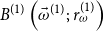 ${B^{(1)}}\left( {{{\vec \omega }^{(1)}};\,r_\omega ^{(1)}} \right)$
,
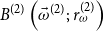 ${B^{(2)}}\left( {{{\vec \omega }^{(2)}};\,r_\omega ^{(2)}} \right)$
and the so-called resistance levels
 $r_\omega ^{(1)}$
,
 $r_\omega ^{(2)}$
are defined as follows:
 \begin{align*}\left\{ {\begin{array}{*{20}{c}}{{B^{(1)}}\!\left( {{{\vec \omega }^{(1)}};\,r_\omega ^{(1)}} \right) = \mathop \sum \nolimits_{t = {t_0}}^{{t_1}} r_\omega ^{(1)}\left( {\frac{1}{{\omega _t^{(1)} - a_t^{\left( {1,2} \right)}}}} \right)}\\[15pt]{{B^{(2)}}\left( {{{\vec \omega }^{(2)}};\,r_\omega ^{(2)}} \right) = \mathop \sum \nolimits_{t = {t_0}}^{{t_1}} r_\omega ^{(2)}\left( {\frac{1}{{a_t^{\left( {1,2} \right)} - \omega _t^{(2)}}}} \right)}\end{array}} \right.\!,\ \text{with} \left\{ \begin{array}{l}{r^{(1)}_{\omega}} = 0.0001 |{\tilde{l}}|/\left( \mathop \sum \nolimits_{t = {t_0}}^{{t_1}} {\frac{1}{{{\tilde{\omega}}_t^{(1)} - a_t^{\left( {1,2} \right)}}}} \right)\\[15pt]{r^{(2)}_{\omega}} = 0.0001 |{\tilde{l}}|/\left( \mathop \sum \nolimits_{t = {t_0}}^{{t_1}} {\frac{1}{{{a}_t^{(1,2)} - \tilde{\omega}_t^{\left( {2} \right)}}}} \right)\end{array} \right.\!,\end{align*}
where
 $\tilde{\omega}_t^{(i)}$
is the initial value of the second level parameter in year
 $t$
for the
 ${i^{th}}$
population,
 $\tilde{l}$
is calculated using the initial values of all the model parameters.
As suggested in Li & Liu (Reference Li and Liu2020, Reference Li and Liu2021), the resistance levels are determined using the initial value of the log-likelihood function. The above specification implies that each barrier function accounts for 0.1% of the magnitude of at the start of the estimation processFootnote 13. At the end of each iteration, the resistance levels
 $r_\omega ^{(1)}$
and
 $r_\omega ^{(2)}$
are reduced by 15% so that the penalty term contributes less and less to the log-likelihood function as it converges.
A.1 Initial values of
$\omega _t^{\left( i \right)}$

Since
 $\omega _t^{\left( i \right)}$
represents the mortality levels at the ending age
 ${x_1}$
, one may simply set
 $\ln m_{{x_1},t}^{\left( i \right)}$
as its initial values. Nonetheless, in the presence of crossovers in the mortality data
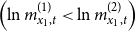 $\left(\ln m_{{x_1},t}^{(1)} \lt \ln m_{{x_1},t}^{(2)}\right)$
in some years, such conditions can violate the requirements of the barrier method (starting from the interior points of the bounds). To avoid such a violation, we employ the following initial values:
 \begin{align*}\left\{ {\begin{array}{*{20}{c}}{\omega _t^{(1)} = \max \!\left( {ln\ m_{{x_1},t}^{(1)},ln\ m_{{x_1},t}^{(2)}} \right)}\\[6pt]{\omega _t^{(2)} = \min \!\left( {ln\ m_{{x_1},t}^{(1)},ln\ m_{{x_1},t}^{(2)}} \right)}\end{array}} \right..\end{align*}
When the sample covers early periods (e.g., before 1970), mortality data at advanced ages may demonstrate some fluctuations. Using the above initial values can result in unreasonable bounds
 $a_t^{\left( {1,2} \right)}$
at the ending age
 ${x_1}$
, which affects the goodness-of-fit. To develop proper constraints, one may also consider using the maximum likelihood estimates (without the no-crossover restrictions) as the initial values.
A.2 Updating equations of
$\omega _t^{\left( i \right)}$

As before, the parameters under the HS4 model are estimated iteratively using the Newton–Raphson method. Combining with the barrier approach, the general updating equation becomes
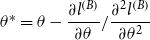 ${\theta ^*} = \theta - \dfrac{{\partial {l^{\left( B \right)}}}}{{\partial \theta }}/\dfrac{{{\partial ^2}{l^{\left( B \right)}}}}{{\partial {\theta ^2}}}$
. Because the barrier functions in
 ${l^{\left( B \right)}}$
are only associated with
 $\omega _t^{\left( i \right)}$
, the updating equations remain the same for the other parameters. The first and second partial derivatives for
 $\omega _t^{\left( i \right)}$
are summarised below:
 \begin{align*}\left\{ {\begin{array}{*{20}{c}}{\frac{{\partial {l^{\left( B \right)}}}}{{\partial \left( {\omega _t^{(1)}} \right)}} = \frac{{\partial l}}{{\partial \left( {\omega _t^{(1)}} \right)}} + r_\omega ^{(1)} \times \frac{1}{{{{\left( {\omega _t^{(1)} - a_t^{\left( {1,2} \right)}} \right)}^2}}}}\\[16pt]{\frac{{\partial {l^{\left( B \right)}}}}{{\partial \left( {\omega _t^{(2)}} \right)}} = \frac{{\partial l}}{{\partial \left( {\omega _t^{(2)}} \right)}} - r_\omega ^{(2)} \times \frac{1}{{{{\left( {a_t^{\left( {1,2} \right)} - \omega _t^{(2)}} \right)}^2}}}}\\[16pt]{\frac{{{\partial ^2}{l^{\left( B \right)}}}}{{\partial {{\left( {\omega _t^{(1)}} \right)}^2}}} = \frac{{{\partial ^2}l}}{{\partial {{\left( {\omega _t^{(1)}} \right)}^2}}} - r_\omega ^{(1)} \times \frac{2}{{{{\left( {\omega _t^{(1)} - a_t^{\left( {1,2} \right)}} \right)}^3}}}}\\[16pt]{\frac{{{\partial ^2}{l^{\left( B \right)}}}}{{\partial {{\left( {\omega _t^{(2)}} \right)}^2}}} = \frac{{{\partial ^2}l}}{{\partial {{\left( {\omega _t^{(2)}} \right)}^2}}} - r_\omega ^{(2)} \times \frac{2}{{{{\left( {a_t^{\left( {1,2} \right)} - \omega _t^{(2)}} \right)}^3}}}}\end{array}} \right..\end{align*}
Appendix B. Tables and Figures
Estimates of multivariate (bivariate) random walk with drift.
 $\hat{{\mu}}$
and
 $\hat{{\sigma}}$
refer to the drift and standard deviation of the fitted processes. Values of the correlation matrix are given in italic.

Fitted (before the dashed line) and extrapolated (after the dashed line) log central death rates under the PS10 model for males in Australia and England and Wales. The dashed line refers to the ending year (2018) of the sample period.

Standard deviation of survivor index
 $S\!\left( {65,t} \right)$
of the cohort aged 65 in 2009,
 $t = 1,2, \ldots ,10$
. The mortality models are calibrated on mortality data in Australia and England and Wales over 1950–2008 and projected/simulated over a 10-year forecasting horizon. Univariate RWD is fitted to the time-varying parameters.