1 Introduction
The Environmental Kuznets Curve (EKC) is an attractive hypothesis as it assumes an inverted-U curve for the relationship between environmental degradation indicators and per capita income. What is implied is that the environmental degradation, though first reinforced with economic growth, is then decoupled from it so that it diminishes once the income level has attained a certain critically high level. Since Grossman and Krueger (Reference Grossman and Krueger1991) first investigated the econometrical evidence for this attractive inverted-U curve, over 100 papers have addressed this topic from different angles: many of them confirm the existence of the EKC, deriving their conclusions from cross-country experience over the last 30 years. However, the credibility of this hypothesis is largely undermined as the various EKC's forms and turning points found in these studies are plagued by incoherence and incomparability. Although the theoretical explanations generally imply that the decoupling between growth and pollution is a rational dynamic trajectory (Lopez, Reference Lopez1994; Antle and Heidebrink, Reference Antle and Heidebrink1995; Kriström and Rivera, Reference Kriström and Rivera1996; Selden and Song, Reference Selden and Song1995; McConnell, Reference McConnell1997; Andreoni and Levinson, Reference Andreoni and Levinson2001; Munasinghe, Reference Munasinghe1999 and Antweiler et al., Reference Antweiler, Copeland and Taylor2001), from a strict econometrical perspective, the reduced-form correlation between income and pollution, which is based on cross-country datasets, could well be ‘spurious’ and is rarely considered to be the ‘optimal’ for each individual country in the datasets. Stern et al. (Reference Stern, Common and Barbier1996) advocated that ‘a more fruitful approach to the analysis of the relationship between economic growth and environmental impact would be the examination of the historical experience of individual countries, using econometric and also qualitative historical analysis’.
However, problems of data availability have largely restrained studies discussing EKC relevance in specific countries. As a result, only a restricted number of papers operate the EKC regression from a single country's time series data. As most of the available environmental data only trace back to the 1960s, the income variation range is often limited. Hence, capturing both the increasing and decreasing stages of pollution trends proves quite difficult. No more than three studies confirm the EKC hypothesis over relatively long historical data series for a single country – namely Roca et al. (Reference Roca, Padilla, Farré and Galletto2001) on Spain (1973–1996), Friedl and Getzner (Reference Friedl and Getzner2003) on Austria (1960–1999), and Lindmark (Reference Lindmark2002) on Sweden (1870–1997). In order to overcome the time-limited data availability constraint, some studies make use of regional disparities in economic growth and environmental quality within the same country: that way, regional-level panel data estimations can be carried out (e.g., Vincent, Reference Vincent1997; List and Gallet, Reference List and Gallet1999; de Groot et al., Reference de Groot, Withagen and Zhou2004). Compared to the studies based on cross-country experience, their assumption about a common trajectory for the income–pollution connection between regions within the same country is more acceptable since the regional characteristics are similar, be they institutional, technical, or structural. Moreover, as these studies focus on all the regions belonging to the same country, problems of omission or of data incomparability on a cross-country level are avoided.Footnote 1 Most of these studies reveal sharp contrasts between country-specific EKCs with respect to the cross-country experience. They also indicate that the advent of a decoupling trend between pollution and income is actually determined by country-specific characteristics as well as by some special events that happened during the investigated time periods, be they technical and structural progress or external shocks such as the oil crisis.
The necessity for a developing country such as China to understand the structural mechanisms of pollution trends during a period of economic growth is two-fold. First, concerning the EKC hypothesis, empirical findings based on international experience generally predict the environmental situation will improve after the per capita income has attained the range of 4000–8000 US$ (1985 price, PPP)(e.g., Grossman and Krueger, Reference Grossman and Krueger1995; Selden and Song, Reference Selden and Song1994; Shafik, Reference Shafik1994). Yet, even with its rapid economic growth, in 2003 China's per capita GDP was only 2,387 US$ (1985 price, PPP). Does this mean a continuous environment deterioration trend cannot be avoided throughout the course of China's further economic growth? And, if so, will the threshold of irreversibility for China's environmental carry capacity be attained, thus jeopardizing the sustainability of China's economic development?
Secondly, some economists suspect that the EKC derived from cross-section data may only be a side effect of trade liberalization, which works as a channel for developed countries to discharge their environmental burden on to developing ones (Pethig, Reference Pethig1976; Chichilnisky, Reference Chichilnisky1994; Copeland and Taylor, Reference Copeland and Taylor1994). According to this hypothesis, trade liberalization would cause developed countries to lose their competitiveness in polluting sectors, so that developing countries, with their lesser environmental regulations, would take over in these sectors. Cole (Reference Cole2004) derived direct empirical evidence for this idea from the experience of OECD countries between 1980 and 1997. In that case, ‘simple’ EKCs have relatively lower turning points than the EKC estimated after the net dirty import from non-OECD countries as a proportion of their total consumption has also been included in the estimation function. Another telling example is Stern and Common (Reference Stern and Common2001) vs. Selden and Song (Reference Selden and Song1994). With just the 22 OECD countries’ data, Selden and Song (Reference Selden and Song1994) found an EKC whose turning point ranged between $8,000 and $10,000. Stern and Common (Reference Stern and Common2001) enlarged the database to include 73 countries as well as most of the new data in connection with developing countries. Their conclusion reveals that the ‘turning point (of the EKC) becomes quite high when the data of developing countries are included or separately estimated’. If their OECD sub-sample still yields an EKC turning point ($9,181) that is similar to the one in Selden and Song (Reference Selden and Song1994), the global and non-OECD countries samples actually reveal much higher turning points: $54,199 (global) and $34,3689 (non-OECD). Considering China's economic growth over the last 25 years has largely been boosted by international trade, if trade liberalization induces China to specialize in polluting industries, should we expect for that country an even higher EKC turning point than for its developed trade partners? Given the current globalization trend, what will the future global environmental situation be if most developing countries follow China's example and face more and more difficulties in bridging the gap between economic growth and pollution?
This paper aims at investigating the EKC hypothesis for China, with provincial industrial SO2 emissions data from 1992 to 2003. Both the reduced and structural models will be tested for per capita emissions, total emissions and emissions density indicators. In the structural model, pollution determinants are first identified as scale, composition, and technique effects; the trade effect will then be included. This is, to our knowledge, the first paper directly investigating the various structural determinants of pollution within the framework of the EKC hypothesis and the model of Antweiler et al. (Reference Antweiler, Copeland and Taylor2001) for a specific developing country – China. The comparison between per capita emissions, total emissions, and emissions density is also carried out, for the first time, in such a straightforward way.
The estimated China-specific EKC curve for per capita industrial SO2 emissions predicts the turning point at 9,500–10,000 yuan (3,085 US$, PPP). However, given China's fast population expansion, the decreasing trend in per capita emissions may well not bring about an immediate reduction in total industrial SO2 emissions. Using the structural EKC model makes it possible to reveal how various factors contribute towards the industrial SO2 emissions density – namely the three commonly known structural determinants: scale, composition, and technical effects, but also the marginal impact of international trade. The latter is actually composed of a significantly negative direct impact and of two indirect ones, which depend on the current capital–labour abundance ratio as well as on the present income level of the province.
The paper is organized as follows. After explaining the choice of the pollution indicator, we first test for the existence of a reduced-form EKC for industrial SO2 emissions in China by using the provincial panel data from 1992 to 2003. In a second step, the structural determinants of industrial SO2 emissions are econometrically decomposed. Thirdly, to analyze the direct and indirect part played by international trade in determining emissions, trade intensity (defined as the ratio of international trade to GDP for the same period) is included into our estimation model, both on its own and in interaction with the other structural determinants. Finally, we conclude.
2 Is the EKC relevant for industrial SO2 emissions in China?
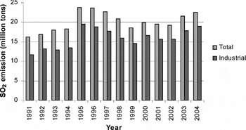
In this paper, industrial SO2 emissions were chosen as the environmental indicator for three reasons. First, SO2 emissions are the biggest air pollution problem in China. In over one-third of Chinese big cities, the SO2 concentration levels are at least twice as high as the 60μg/m3 standard set by the World Health Organization (WHO) for developing countries SEPA (1998–2002). The potential negative impact of there emissions on public health is beginning to be well documented, especially as a significant cause of respiratory diseases (Xu et al., Reference Xu, Gao, Dockery and Chen1994; World Bank, 1996a). Moreover, due to SO2 emissions, the ever-expanding acid rain problem in both South and North China has also resulted in rapid reduction in equipment and soil productivity (World Bank, 1996b). Second, SO2 emissions are generally believed to be the local pollution factor that is most likely to develop an inverted-U relationship with income growth. Therefore, by focusing on SO2 pollution, we expect to get more references and terms of comparison for our results. Finally, as shown in figure 1 with historical statistics, over 75 per cent of SO2 emissions in China derive directly from industrial sectors and total SO2 emissions variations were also mainly caused by variations in industrial sectors, while the amount of emissions from other sources remained relatively stable. Furthermore, general omission is observed for the total SO2 emissions statistics at a provincial level for 1996–1997. For all these reasons, it seems relevant to focus on the industrial SO2 emissions case.
Evolution of SO2 emissions in China during economic reform period Data Sources: China Energy Databook 6.0 and SSB (various issues)

As in most of the papers discussing the EKC hypothesis, we first investigate the existence of an inverted-U curve for per capita industrial SO2 emissions. However, our analysis will focus more on the determinants of industrial SO2 emissions density. This indicator is calculated by dividing annual industrial SO2 emissions by the surface of the province. This environmental indicator has two main advantages. Firstly, as the geographical surface of each province is a constant number, this indicator preserves the dynamic characteristic of total industrial SO2 emissions for each province. That point is at the core of environmental economic studies since the environmental quality and carry capacity of the ecosystem are both determined by the total volume of emissions, and not by per capita emissions. Secondly, Antweiler et al. (Reference Antweiler, Copeland and Taylor2001) tested their pollution determination model by using the pollution concentration indicators. However, at an international level, concentration indicators are often collected at city level, while economic statistics only exist at country level; as a result, Antweiler et al. (Reference Antweiler, Copeland and Taylor2001) had to carry out a regression of city level pollution concentration indicator on the country average level economic determinants, which, to some extent, weakens their results. As a measurement, emissions density is close to pollution concentration, especially for SO2 emissions, which are widely regarded as a local pollutant. Moreover, as opposed to pollution concentration, emissions are also caused directly by economic activities. Considering these aspects, we believe using industrial SO2 emissions density will permit us to capture the direct link between economic activities and pollution results, and to obtain more credible estimation results for the structural emissions determination model.
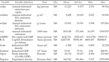
Table 1 summarizes the statistics for all the data used in the emissions determination analysis in sections 2 to 4. As the panel database encompasses 29 provinces for the 1992–2003 period – the main period of economic reform in China – we observe a wide spectrum of values for both pollution and economic indicators, which is a necessary condition for robust EKC estimates.
Statistic description on the data used in EKC analysis

Notes: 1. All the variables measured in value are converted into the yuan of 1990 constant price.
2. The total industrial capital stock is calculated by permanent inventory method by using real value of fixed investment data (on the constant price of 1990) of each province in each year deflated by the corresponding fixed investment price index. More details about the permanent inventory method are in Wu (Reference Wu and Tsu-Tan1999).
3. The export and import data are on the whole provincial economy level instead of the provincial industrial economy level. As we are actually interested in the impact of international trade on emissions, we do not think it is necessary to use the industrial economy-level trade data.
4. Data sources: SSB (1985–2004).
We first examine whether an ‘inverted-U’ relationship exists between per capita SO2 emissions and per capita income. At this stage, the equation used is a simple reduced-form estimation function (2), which directly connects per capita SO2 emissions (so2pc it) with GDP per capita (GDPPC it)

Indices i and t respectively stand for the province and year. Xi represents the non-measurable constant province-specific effect. βt is the time-specific intercept used to account for the stochastic shocks common to all the provinces over the same period. Observing that most of the previous EKC studies included population density as an independent variable on the right-hand side of the EKC estimation function, we have added this variable.Footnote 2 Considering the ‘public bad’ characteristics of air pollution problems, we believe a higher population density tends to intensify the negative impact of air pollution. Hence, provinces with higher population densities should have fewer pollution problems when compared with a province which has the same income level but a lower population density. We therefore expect a negative coefficient for this variable.
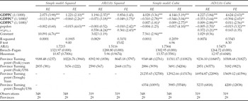
The main EKC estimation results for per capita industrial SO2 emissions are reported in table 2. Both random and fixed effect estimators are used for panel data. The simple model columns report the estimates based directly on equation (1) while the AD(1,0) columns list the results in which the first-order serial-correlation problem is corrected by including the instrumented lagged dependant variable so 21pc it–1 on the right-hand side of the estimation function.Footnote 3 To test for the possible re-increasing trends of the EKC after the dichotomy between economic growth and pollution has been achieved, we also estimate the cubic EKC model. As opposed to what is usually reported for international experience, our estimation results display relatively good stability for model and estimation method changes. Though the cubic model predicts a re-increasing trend for per capita industrial SO2 emissions after the per capita GDP has attained a relatively high level (13,000–17,000 yuan, or 4,600 US$, 1985 constant price, PPP), the location of its peak turning point matches what is found with the squared model. Both models expect the dichotomy between per capita economic growth and per capita industrial SO2 emissions to be achieved once the per capita GDP has attained 9,500–11,000 yuan (1990 constant price, which is equal to 3,085 US$ according to purchasing power parity or 1,215 US$ according to official exchange rate, 1985 constant price of US$).Footnote 4 As expected, population density plays a significant part in curbing pollution emissions, although its impact remains relatively small.
EKC Industrial SO2 emissions per capita
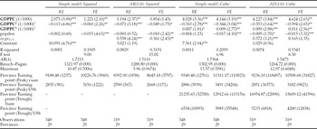
Notes: Absolute value of z statistics in parentheses, °significant at 15%, *significant 10%, **significant 5%, ***significant 1%.
The standard error of the turning point is indicated in the parentheses below. They are calculated by Delta method. See Greene (Reference Greene1999: 913–914) for details.
FE means fixed effect, and RE means random effect.
AR (1) is the Durbin–Watson statistics for first order serial correlation. Breusch–Pagan is used to test the group specific effect. Hausman test is used to compare the efficiency between fixed and random panel data estimator.
The instrumentation method employed in AD (1,0) model for so 2pc t−1 is developed by Balestra–Nerlove (Reference Balestra and Nerlove1966) for the ‘fixed effect of the dynamic linear penal model’.
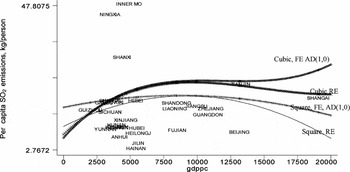
The estimated EKC is shown in figure 2, together with the location of the 29 provinces. Except for provinces with higher incomes such as Shanghai, Beijing, Tianjin, Guangdong, and Zhejiang, most of the provinces are still on the increasing track of the EKC by year 2003; hence, according to the EKC hypothesis, increasing pollution problems should be expected.
Estimated EKC for per capital industrial SO2 emissions and the actual location of the 29 provinces in 2003 (based on the estimation results of table 2)

Then, the EKC hypothesis is considered for the case of industrial SO2 emissions density. At this stage, we use the same EKC model as in equation (2): it includes both the per capita income terms and population density.

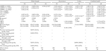
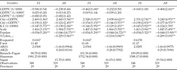
The estimation results based on this function are reported in table 3. In contrast with per capita emissions, it appears that industrial SO2 emissions density data do not support the EKC hypothesis. In the three estimations based on the whole of the 29 provinces sample, neither the squared nor the cubic model yield significant coefficients for income terms. A significantly positive coefficient (0.391) is only found for income term in the linear model. Does this mean economic growth always leads emissions density to increase in China?
Nexus between industrial SO2 emissions density and per capita GDP

Notes: Absolute value of z statistics in parentheses, °significant at 15%, *significant 10%, **significant 5%, ***significant 1%.
The standard error of the turning point is indicated in the parentheses below.
In the spline model, we distinguish the coefficient of income terms between cities and province. The income coefficients for province are those before the simple GDPPC terms. But to obtain coefficients of income term for 3 cities, we need to add the GDPPC and GDPPC×city together.
AB means Arellano–Bond (Reference Arellano and Bond1991) dynamic GMM estimator for fixed-effect panel data. In this estimation method, the statistic value of AR(2) denotes the second order serial correlation.
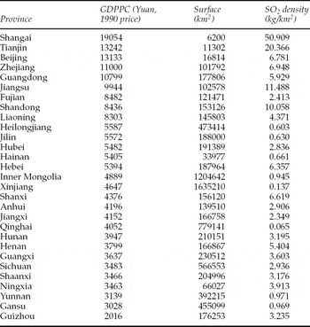
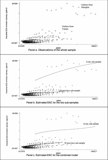
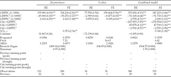
Two factors come into play to determine emissions density: the province's total annual emissions quantity is the numerator and the province's surface is the denominator. The reason why this indicator does not support the EKC hypothesis may reside in this two-fold aspect. In table 4, in decreasing order of per capita GDP, we list for each of the 29 provinces their income levels, geographical surfaces, and industrial SO2 emissions density data in 2003. Interestingly, all three indicators for the three municipalities directly placed under central government – namely Shanghai, Beijing and Tianjin – seem very different from those of the other 26 provinces. These three cities boast relatively higher per capita income levels, but they also happen to have the smallest geographical areas. Therefore, their SO2 density levels are naturally much higher than those of other provinces. We can come to the same conclusion with panel a. in figure 3: almost all the observations for the 26 provinces are concentrated in the bottom-left part of the diagram while the few exceptional points in the top-right part refer to the other three municipalities. So, is the linear positive relationship between SO2 density and income simply caused by the inclusion of the observations related to the three cities?
Provincial per capita GDP, geographical area statistics and emissions density

EKC estimations for the industrial SO2 emissions density

To test for this hypothesis, the database is divided into two sub-samples – 26 provinces and three cities – and the estimation is redone. The results are also reported in table 3 and their graphical illustrations are given in panels b and c in figure 3. At this stage, we use both the Balestra–Nerlove method (Reference Balestra and Nerlove1966) and the first-difference general methods of moments (GMM) for linear, dynamic panel data. That method proposed by Arellano and Bond (Reference Arellano and Bond1991) tackles serial correlation problems.Footnote 5 The estimates for both the 26 provinces and three cities sub-samples still predict an increasing tendency for China's industrial SO2 emissions density during the economic growth process.Footnote 6
The last two columns in table 3 report the estimates of a combined model in which a spline structure is used so that the estimation may be applied to the whole database, all the while distinguishing the potential income coefficient differences between the 26 provinces and the three cities.Footnote 7 Once more, the combined model confirms the common increasing trend for industrial SO2 density. Furthermore, the increasing trends are very similar for the 26 provinces and for the three cities, except that the absolute emissions density level is much higher for the latter (cf. panel c, figure 3).
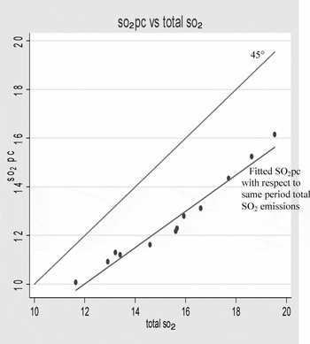
Population expansion may account for the fact that the inverted-U curve for per capita industrial SO2 emissions seems to co-exist with the monotonically increasing tendency for industrial SO2 emissions density. Figure 4 plots in a two-dimension diagram the trends for per capita industrial SO2 emissions and total industrial SO2 emissions on a national level in China between 1992 and 2002. If the size of the population remained unchanged, a one-to-one correspondence could be expected between the variations of SO2 emissions and per capita SO2 emissions, as represented by the 45° diagonal line. However, both the per capita SO2 emissions plotted with respect to total SO2 emissions and the fitted correlation between them reveal a less than one correlation. This actually implies a fast population expansion, which would slow down the increasing tendency of per capita SO2 emissions compared to that of total SO2 emissions. Therefore, for the case of China, the divergence in the trends of industrial SO2 density and per capita SO2 emissions are actually similar to that mentioned in Stern et al. (Reference Stern, Common and Barbier1996); although per capita emissions peaks relatively early, the total volume of emissions will keep on increasing under the pressure of population expansion. This is further confirmed by the EKC estimation results for total industrial SO2 emissions reported in table 5, which also predicts increasing trends for total industrial SO2 emissions in both the 26 provinces and the three cities.
Comparison of the evolution of per capita SO2 and total SO2 emissions (National level: 1992–2002) Source: China Statistical Yearbook

Total industrial SO2 emissions EKC reduced model
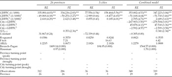
Notes: Absolute value of z statistics in parentheses, °significant at 15%, *significant 10%, **significant 5%, ***significant 1%.
The standard error of the turning point is indicated in the parentheses below.
3 Industrial SO2 emissions and its structural determinants
In the last section, it appears that EKC analyses cannot dispel our concerns about the continuously deteriorating industrial SO2 pollution situation in China, even if the turning point for per capita industrial SO2 emissions proves to come earlier than international experience would have it. Thus, in this section, the potential structural determinants of pollution are investigated with a view to detecting those that contribute towards the continually increasing trend of industrial SO2 emissions.
The structural model
Grossman decomposition adaptated to our provincial level panel data
If it is agreed that emissions are a by-product of production, according to Grossman (Reference Grossman, Goldin and Winter1995), the industrial SO2 emissions in each province i during period t can be written as a product of its three determinants in equation (3).
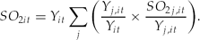
The index j = 1, . . ., n stands for various industrial sectors. Yit presents the total industrial GDP in province i during period t and SO2it is the total industrial SO2 emissions for the same province. Y j, it is the GDP generated in industrial sector j of province i during period t and SO2j, it is the corresponding sector-level SO2 emissions.
Following section 2, our investigation will first focus on the determination of industrial SO2 density in each province. Therefore, we divide the time-invariable provincial surface (areai) on both sides of the equation (3) and obtain

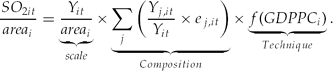
The first term on the right-hand side of equation (Yit/areai) becomes the industrial activity density. (Yj,it/Yit) gives the proportion of product for sector j in the total industrial product of province i. Finally, the term (SO 2j, it/Yj,it) calculates the sector-specific pollution intensity. If we suppose that it (SO 2j, it/Yj,it) can be represented by provincial-level average emissions intensity (SO 2it/Yit) adjusted by a sector-specific emissions efficiency indicator, ej, it, we have  . Equation (4) is then transformed into
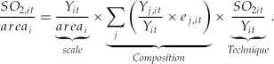
The three structural determinants of emissions are now easy to distinguish in equation (5). The term (Yit/areai) corresponds to scale effect.Footnote 8 Higher industrial activity density normally means higher emissions density providing other factors remain constant. With the inclusion of the sector-specific emissions efficiency indicators ej,it the other two effects can be distinguished. Firstly, the provincial-level average SO2 emissions intensity (SO 2it/Yit): it measures the technical effect. Lower emissions intensity will result in lower emissions density, all else equal. Secondly, the composition effect 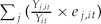 . If we first suppose the sector-specific emissions intensity remains at its original level ej,it −s1, while the proportion of polluting sectors increases – their emissions intensity being higher than provincial average – that is ej,it −1>1, we obtain a new composition effect term at period t as
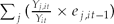 , which must be bigger than
 . This actually gives us a way to present composition-related emissions increases.Footnote 9
Relationship between industrial SO2 emissions intensity and income: can we use per capita GDP to extrapolate technical effect?
To transform the decomposition function (5) into an estimable model, however, we face one difficulty. Although both scale and composition effects can be directly measured by economic statistic indicators in the estimation function, as far as technical effect is concerned, provincial-level average industrial SO2 emissions intensity cannot be used directly as a measurement because of potential endogeneity.Footnote 10 We therefore need to find an economic indicator that is closely related to technical effect but does not involve industrial SO2 emissions in its measurement.
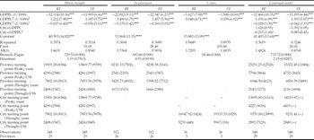
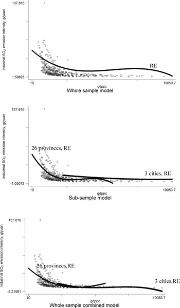
Among the previous empirical structural analysis concerning pollution determination, Selden and Song (Reference Selden and Song1994), Panayotou (Reference Panayotou1997), and Cole and Elliott (Reference Cole and Elliott2003) have used per capita GDP as extrapolation for technical effect. To see whether per capita GDP can also be served as a good approximate for technical effect in the case of China, we check the direct correlation between per capita GDP and provincial level average industrial SO2 emissions intensity. The estimation results are reported in table 6. As in section 2, the potential coefficient difference is also distinguished between the three big cities and the 26 provinces. In figure 5, we have the corresponding graphical demonstration for the estimated relationship. What can easily be observed is a common decreasing tendency in industrial SO2 intensity with respect to income growth. Although there is a slight fluctuation on the border of some income level samples, we believe that, globally, per capita income growth has a negative correlation with industrial SO2 emissions intensity. Therefore, it can be served as a suitable extrapolation for trends in pollution-abatement technology, and a negative coefficient for this variable can be expected. So we have
Relationship between per capita GDP and Industrial SO2 intensity

Notes: Absolute value of z statistics in parentheses, ° significant at 15%, *significant at 10% **significant at 5%; ***significant at 1%.
The standard error of the turning point is indicated in the parentheses below. The – that appears in the last column shows the non-convergency of the results due to the very low significance of the estimated coefficients.
Correlation between GDPPC and industrial SO2 emissions intensity

The structural estimation function
Based on equation (6), we obtain the estimation function to investigate the structural determination of emissions density

On top of the GDPPC and its polynomials to measure the technical effect, we use provincial total industrial GDP density (Scaleit/areai) to measure the scale effect. The same measurement has also been employed in Kaufman et al. (Reference Kaufmann, Davidsdottir, Garnham and Pauly1998) and Antweiler et al. (Reference Antweiler, Copeland and Taylor2001) in their investigation on the structural determinants of certain air pollution concentration indicators. We expect a positive coefficient for it. Cole and Elliott (Reference Cole and Elliott2003) have used per capita emissions as the dependant variable to investigate the structural determinants of the EKC. However, this obliges them to use per capita GDP to capture both technique and scale effects. Here the advantages for us to use industrial SO2 emissions density as the dependant variable are actually two-fold. Firstly, as we concentrate on the SO2 emissions caused by industrial production, the scale effect can be distinguished clearly from technical effect, since the former is measured by total industrial GDP and the latter is measured by per capita GDP. Secondly, using the density of industrial SO2 emissions as the dependant variable also helps us reduce the potential correlation between total industrial GDP and per capita GDP, since the former is now deflated by the geographical surface of each province and the latter by its population size.Footnote 11
The original idea for the measurement of composition effect in equation (7) requires detailed statistics on sector-specific emissions intensity and added value. However, only sector-level added value data are available in China. We therefore need another approximate for composition effect. Considering this structural model is very similar to that proposed by Antweiler et al. (ACT, 2001), we decide to follow their example and use the capital-abundance ratio (K/L)it to describe composition effect for each province. The implicit assumption behind this extrapolation is that a sector whose production procedures require more capital should be more pollution intensive.Footnote 12 Therefore, a positive coefficient is expected for this variable.
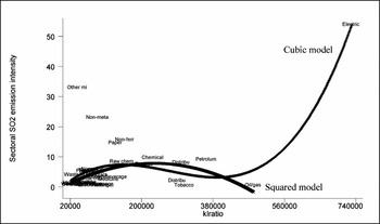
Correlation between sector-level capital-abundance ratio and SO2 emissions intensity

The structural model and its estimation results
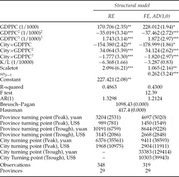
The estimation results based on equation (7) are reported in table 7. Following section 2, for the technical effect, we keep using the spline combined function form to distinguish the potential coefficient difference between the 26 provinces and the three big cities. Only gradually do we delete the insignificant polynomial income terms during the estimation process.
Structural model and decomposition results (Industrial SO2 emissions density)
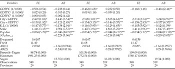
Notes: °significant at 15%, *significant at 10% **significant at 5%; ***significant at 1%. Absolute value of z statistics in parentheses.
The standard error of the turning point is indicated in the parentheses below.
FE means fixed-effect estimator for panel data. AB represents Arellano–Bond (Reference Arellano and Bond1991) dynamic GMM estimator for fixed-effect panel data.
The inclusion of the structural and scale characteristics into the determination of industrial SO2 emissions density obviously improves the power of explanation of the whole model; the adjusted R2 value increases from 0.50 (cf. table 3) to 0.62. The more satisfactory statistics for the auto-correlation test reveal that the serial correlation problem observed in the previous EKC analyses may be simply caused by variable omission. The positive coefficient before the scale effect confirms our expectation; higher industrial activity density does predict higher industrial SO2 emissions density. However, the significant but negative coefficient obtained for the capital-abundance ratio (K/L)jt is contrary to our original expectation and to the general conclusion obtained from international experience.
One possible explanation for this contrary-to-intuition result is that the industrial sectors employing capital more intensively are not necessarily the most polluting ones. Figure 5 illustrates such a possibility, plotting China's 39 industrial sectors into a diagram according to their capital-abundance ratio and SO2 emissions intensity data in 2004. Clearly, except for the electricity generation sector for which capital-abundance ratio and pollution intensity indictors are both extremely high, the correlation between the capital-abundance ratio and sector SO2 emissions intensity is not a linear positive one for the other 38 sectors. Although for the most labour-intensive sectors, a higher capital–labour ratio means higher emissions intensity, once the capital-abundance ratio has attained a certain level (showed by the squared and cubic model estimated according to the 39 points of observation), a high capital–labour ratio might also lead emissions intensity to decrease. This finding actually echoes that of Dinda et al. (Reference Dinda, Coondoo and Pal2000) who showed the potential ambiguity in using capital abundance as a measurement for industrial composition, since the ‘capital intensive sector could also be more likely to be clean technology owner’.
Concerning the technical effect, the spline estimation function still reveals that results differ for the 26 provinces and the three cities. While a linear negative correlation between GDPPC and SO2 emissions density is found for the 26 provinces with the Arellano–Bond GMM estimation, it is not so for the three cities. For them, the combined correlation between emissions density and per capita income can only partially be decomposed into scale and composition effects – the coefficients obtained for the income terms for the three cities still predicts an inverted-U curve, but the turning point decreases to the range of 7,900–8,400 yuan (vs. 27,033 yuan reported in table 3). This divergence between provinces and big cities can be partly accounted for by structural differences: as the industrial production in the three cities might be more consumption-led than that in the other 26 provinces, a dichotomy between economic growth and pollution reduction should be more difficult to achieve.
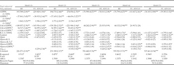
For the sake of comparison, the structural determination model is also applied to the case of total industrial SO2 emissions. In that perspective, we use the total industrial GDP of each province (scale it) to measure the scale effect. The estimation results are reported in table 8. Although the decomposition effect is less efficient than for industrial emissions density, the results prove relatively stable. They confirm the positive scale effect and the unexpected negative composition effect, as in the case of emissions density. The poor efficiency of decomposition is more general – including scale and composition effects into the estimation fails to reveal the expected negative relationship between emissions and technical effects for both province and city groups, but as in the case of emissions density, the inverted-U curves that remain between emissions and per capita GDP generally predict much lower turning points.
Structural model and decomposition results (Total industrial SO2 emissions)

Notes: °significant at 15%, *significant at 10% **significant at 5%; ***significant at 1%. Absolute value of z statistics in parentheses.
The standard error of the turning point is indicated in the parentheses below.
4 Is international trade good for the environment in China?
The persistence of an inverted-U shape for the emissions–income relationship in the structural model for both emissions density and total emissions reminds us of the limited decomposition efficiency of the structural model proposed in section 3. We suspect that some structural determinants are still left out of the model.
If the ‘Pollution Haven’ hypothesis holds, international trade should also be a major emissions determinant for China. Compared to developed countries, China is both well-off for labour and less rigorous in terms of pollution control regulation. Following the reasoning of Copeland and Taylor (1995), we can expect that China's natural comparative advantages will, on the one hand, lead it to specialize in labour-intensive sectors, which are often supposed to be less polluting; but, on the other hand, with less stringent environmental regulations, it may well specialize in pollution-intensive sectors. The global effect of trade upon environment should, therefore, depend on the force-contrast between the natural comparative advantage measured by factor-endowment and the environmental comparative advantage measured by relatively less strict environmental regulations.
In this section, the empirical model of Antweiler et al. (ACT, 1998, 2001) is used to check how trade impacts on China's industrial SO2 emissions. The estimation function can be illustrated with equation (8).

Indeed, this equation is an extended version of the estimation function (7) used to investigate the structural determinants of industrial SO2 emissions. The five extra terms included here appear on the second line of (8).
The simple trade intensity variable (openjt) is measured by the ratio of the sum of exports and imports over the total GDP ((X+M)/GDP). This term is included in order to trace the direct impact of trade upon industrial SO2 emissions.Footnote 13 The multiplicative terms of trade intensity (openjt) with the capital–labour abundance ratio (K/L)jt and per capita income GDPPCjt are also introduced – they can help capture the force-contrast between the factor-abundance and ‘pollution haven’ motive to determine the changes in China's composition.Footnote 14 Following ACT (2001), we also make the squared per capita income GDPPCjt 2 and squared capital–labour ratio (K/L)jt 2 interact with the trade intensity ratio in equation (8). As explained in ACT (2001), with the force-contrast between the comparative advantages of these two differing aspects, theory fails to reveal at what point further increases in the capital-abundance ratio may cause pollution to rise or when increases in per capita income may finally cause pollution to decrease. Using this flexible interactive structure, we expect the interacted quadratic capital–labour abundance ratio with trade intensity will imply an emissions-increasing impact of trade for high capital–labour ratio, and an opposite effect for lower ratios. This corresponds to the situation where, regardless of Chinese provinces’ other characteristics, if their capital–labour abundance ratio is sufficiently low with respect to that of their trade partners, they must export clean goods. Conversely, if their capital–labour ratio is not low enough, they might be able to export polluting goods, given their weaker environmental regulations. Similarly, we expect the interacted quadratic per capita income to go with a pollution-reducing impact of trade when the provincial income is relatively high, while it is expected to go with a pollution-increasing impact when it is relatively low. This actually corresponds to the fact that, if a province's per capita income is low enough, it may export polluting goods even if its comparative advantages are in labour-intensive sectors. Conversely, if its income is not so low, it may carry on producing in labour-intensive sectors that are generally cleaner.
Note that, as opposed to ACT (2001) as well as Cole and Elliott (Reference Cole and Elliott2003), we use the provincial-level absolute capital–labour abundance ratio and per capita income in the trade-related multiplicative terms rather than the relative K/L and per capita income with respect to their sample average value. This is because our point of interest lies with the international trade developed by each Chinese province with all the other foreign countries. Therefore, what determines the comparative advantages of each province is the gap between its K/L and per capita income and those for the world average (excluding China). However, since the world average terms are actually the same each year for all the provinces, including them would only alter the scale of the coefficients for the multiplicative terms, but would not change their essential relationship. The only reason to make this arrangement here would be that China's economic growth and capital accumulation rate are both relatively higher than the world average, so that, over time, what should be expected is a gradual reduction of these gaps. Yet, since our estimation only covers 12 years, we do not believe this arrangement can make a significant difference in the estimation results.Footnote 15
We run the estimation for both industrial SO2 emissions density (cf. table 9) and total industrial SO2 emissions (cf. table 10), the way that, in table 8, the industrial GDP is used to measure the scale effect for the estimation on total emissions.
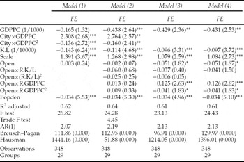
ACT (1998) structural model: trade–environment nexus request (29 provinces, 1992–2003)

ACT (1998) structural model: trade–environment nexus request (29 provinces, 1992–2003)

Note: Arellano and Bond (Reference Arellano and Bond1991) dynamic GMM estimation method is not used in this table due to its significant incapability in removing the serial correlation between the time serials of the same group.
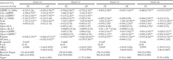
Let us first examine the results concerning emissions density. In all the columns, the inclusion of trade intensity variables does not affect the coherence of the estimated coefficients for emissions’ three basic structural determinants. The scale effect keeps its around-one positive coefficient. Concerning the capital–labour abundance ratio, as an approximate measure for composition effect, the counter-assumption significantly negative coefficients are still there.
Model (1) only includes the direct determinant role of the openness factor. The estimation results for the full model illustrated by equation (8) are reported in the following columns. If we keep using the spline model to tell the difference between provinces and big cities in model (2), we fail to obtain significant coefficients for all the openness-related terms. However, there is an obvious decrease for the significance of the coefficients in the spline structure when the trade-related terms are included (cf. tables 7 and 8). At the same time, a collective significant F-test is obtained for the five trade-related terms: the value is 4.7 for the fixed-effect (FE) estimation, and 10.91 for the Arellano–Bond (AB) dynamic GMM estimation. We suspect the trade-related terms and the spline structure for technique effect may be multi-collinear. Therefore, in model (3), the spline structure for the technique effect is removed from the estimation. As a result, while the power of explanation of the model remains unchanged, the trade-relative terms become significant once the spline structure of the technique effect has been removed. We take this to imply that the trade characteristic of the provincial economy helps to accomplish the structural decomposition of the EKC, as discussed in the last section. After the inclusion of the five trade-related terms, we finally succeed in obtaining a general negative coefficient for the per capita GDP which measures the pure technique effect.
Trade openness, once collectively included into the other trade-related multiplicative terms, seems to have a direct pollution-reducing impact. This actually matches the findings based on international experience by ACT (2001) and Cole and Elliott (Reference Cole and Elliott2003). The estimation results for the interactive terms between trade and comparative advantage characteristics generally confirm ACT's theoretical expectation, with the exception of the relatively weak significance of the trade-(K/L) multiplicative term, especially with the Arellano–Bond GMM estimation.Footnote 16 At a provincial level, if the K/L ratio is lower than 890,000 yuan/person according to FE estimation or to 416,667 yuan/person with the Arellano–Bond estimator, then its SO2 emissions falls with trade liberalization. While for a province whose per capita GDP is lower than 8,000 yuan according to the fixed effect estimation or to 11,000 yuan according to the GMM estimation, more trade openness results in a growing industrial SO2 emissions density, since their comparative advantage in dirty production becomes more acute.
Although the coefficients are relatively less significant, the estimation results reported in table 10 for total industrial SO2 emissions are in tune with those of emissions density. As in the case of emissions density, including trade intensity does not affect the stability of the coefficients for scale, composition, and technique effects. The simple trade intensity term is also proven to be an emissions-reducing factor. Moreover, we also observe similar force-contrast patterns between the factor-endowment-based comparative advantage and pollution haven hypothesis. The strong coherence between the results obtained for various pollution measurements reveals the good stability of the structural model proposed by ACT (2001).
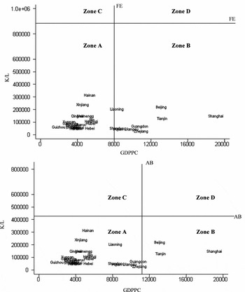
Figure 7 reports the combinations of the K/L ratio and per capita GDP for the 29 Chinese provinces in year 2003. The horizontal and vertical lines FE and AB divide the K/L-per capita GDP diagram into four zones, which represent the possible situations resulting from a combination of the factor-endowment comparative advantage and the pollution haven motive. Clearly, all of the 29 Chinese provinces actually have obvious comparative advantages in less polluting labour-intensive industries.Footnote 17 For most of them, their relatively low income level also endows them with advantages in polluting industries. Only the three cities according to the Arellano–Bond estimation, or the eight richest provinces and cities (Shanghai, Beijing, Tianjin, Guangdong, Zhejiang, Jiangsu, Fujian, Shandong, and Liaoning) according to the FE estimation, have surpassed the phases of the force-contrast between the factor-based and pollution-haven-based comparative advantage.
Actual K/L and per capita GDP situation of the 29 Chinese provinces (2003). Zone A: Pollution haven comparative advantage cancelled out by factor-endowment comparative advantage in cleaner industry. Zone B: Factor-endowment comparative advantages in cleaner industry reinforced by pollution haven comparative disadvantage. Zone C: Pollution haven comparative advantage reinforced by factor-endowment comparative advantage in polluting industry. Zone D: Factor-endowment comparative advantages in polluting industry cancelled out by pollution haven comparative disadvantage

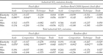
However, illustrating the combination between the endowment-based and the ‘pollution haven’-based comparative advantage in figure 7 fails to give us a precise idea about the role actually played by trade in each province. In fact, the final outcome of the force-contrast between these two comparative advantages should depend on the exact level of per capita income and factor endowment situation in each province (ACT, 2001 and Cole and Elliott, Reference Cole and Elliott2003). To solve this problem, we calculate the elasticity of emissions with respect to trade intensity and its three traditional structural determinants.Footnote 18 Space being limited, we only report in table 11 the elasticity results at a national level for both industrial SO2 emissions density and total emissions. The elasticity results seem reasonable and display good coherence with the decomposition results. Generally speaking, the differences generated by estimation methods for the same emissions determinant do not affect the direction and magnitude of elasticity, except for trade intensity whose elasticity tends not to be as precise. For both emissions indicators, we find a positive and significant elasticity result for scale effect and a negative and significant one for technique effect. Concerning the elasticity of the composition effect, its negative elasticity found in the two emissions cases reminds us again of the unexpected negative correlation between the capital–abundance ratio and pollution. Although the standard error reveals a relatively less significant elasticity for trade intensity, the values of both total industrial SO2 emissions and emissions density for trade elasticity are all very close to zero, ‘no matter positive or negative’, as in ACT (2001). Therefore, in China as in international experience, international trade only plays a marginal part in determining emissions variations.
Scale, composition, technique and trade elasticity

Notes: ***indicates significance at 1% confidence level. **indicates significance at 5% confidence level. *indicates significance at 10% confidence level.
Elasticity is evaluated at the average of the independent variables.
5 Conclusion and discussion
In this paper based on Chinese provincial panel data from 1992 to 2003, we first tested whether the EKC hypothesis was relevant in the case of industrial SO2 emissions density. Then, we decomposed the economical determinants of SO2 emissions into three effects – namely scale, composition, and technique. In a third step, we studied the direct and indirect roles of international trade intensity ((X+M)/GDP).
In comparison with the conclusions found in cross-country studies, the China-specific EKC obtained here seems to predict the advent of a relatively earlier turning point for per capita industrial SO2 emissions at a point when the per capita income has roughly attained 3,085 US$. However, our results also reveal that, given the rapid population expansion in this country, such a seemingly optimistic decreasing trend as the one anticipated by the EKC hypothesis for per capita emissions will not bring about an immediate reduction in the total industrial SO2 emissions – the indicator having more direct impact on China's environmental quality. In a way, we believe the inverted-U-shaped correlation between the per capita GDP and per capita SO2 emissions found in the reduced-form EKC model only reveals some ex-post description. The convincing causality between economic activities and emissions results can only be understood through more structured models. Our study offers new evidence on several points. First, the per capita income no longer appears as the solo determinant in emissions determination, as was the case in the reduced-form EKC model, but rather as a mere pollution-reducing technique factor in the structural models. Second, the efficiency of the model specification has been improved after the other pollution determinants have been included into the structural model.
In accordance with our expectations, the estimation results of the structured model reveal industrial scale enlargement has a pollution-increasing role, while technical progress has a pollution-decreasing one often catalyzed by the reinforced demand for a better environment when people get richer. However, unexpected negative coefficients have appeared for the composition effect measured by capital–abundance ratio –K/L. Although this indicator is generally believed to be a good cross-country environmental performance measurement for industrial structure, the evidence illustrated in this paper with China's sector-based data reveal its ambiguous aspects in terms of structural and technical measurements. Investigations to find a more relevant composition effect measurement might be an interesting continuation for this study.
Analyzing the impact of trade upon environment was an issue inspired by the model proposed in ACT (1998, 2001). Our major results confirm ACT's theoretical analysis. Concerning the role of trade, we find that besides a significantly negative direct impact, its indirect impacts upon emissions depend on the natural factor endowment and environmental regulation situation of each province. Although evidence has been given here in favour of the ‘pollution haven’ hypothesis, it appears trade liberalization still plays a marginal but pollution-reducing role in most cases, since most provinces are richly endowed in terms of labour force. Therefore, to some extent, it can be stated that commercial openness, given China's current specific characteristics, is not likely to undermine China's sustainable development strategy.
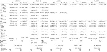
Appendix: Final structural model using relative K/L and relative per capita income
ACT (1998) structural model: trade–environment nexus request (Dependant variable: industrial SO2 emissions density

Notes: We do not report AB results due to the unsatisfactory efficiency of its instrumentation step.
R.KL means the relative capital-abundance ratio with respect to world average level and R.GDPPC means the relative per capita GDP with respect to world average level. The data about the world average K/L and GDPPC of each year is compiled by author from World Development Indicator. Following are their statistic descriptions.

ACT (1998) structural model: trade–environment nexus request (Dependant variable: total industrial SO2 emissions)

R.KL means the relative capital-abundance ratio with respect to world average level and R.GDPPC means the relative per capita GDP with respect to world average level. The data about the world average K/L and GDPPC of each year is compiled by author from World Development Indicator (2004).
 , which equally means
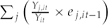 > 1. This reflects the increase of total emissions purely caused by structural changes in production.