

Statistical moderation has been central to theoretical accounts of risk, resilience, and (mal)adaptation from the beginning of its formal study (Garmezy, Masten, & Tellegen, Reference Garmezy, Masten and Tellegen1984). Indeed, in many respects the study of resilience is by definition the search for protective factors that moderate the impact of psychosocial stressors on development (Luthar, Cicchetti, & Becker, Reference Luthar, Cicchetti and Becker2000; Masten, Reference Masten2001). Similarly, one of the dominant models of risk and developmental adaptation—the diathesis–stress or dual-risk model—explicitly posits moderation (Heim & Nemeroff, Reference Heim and Nemeroff1999). Specifically, the diathesis–stress model suggests that poor developmental experiences (e.g., low quality parenting) are most likely to impact the development of individuals who carry vulnerability factors, which are latent diatheses that result in maladaptation when “triggered” by poor experience. Many potential diatheses have been the focus of empirical inquiry, including temperamental traits, such as difficulty (Belsky, Hsieh, & Crnic, Reference Belsky, Hsieh and Crnic1998), and specific molecular genetic polymorphisms, such as the short allele of the serotonin transporter gene (Caspi et al., Reference Caspi, Sugden, Moffitt, Mill, Taylor and Craig2003).
One common theme in this research is that such moderators are “vulnerability factors” that inhibit successful adaptation in the face of adversity. Thus, one of the more important developments in the last decade is the evolutionary psychology-inspired theory of differential susceptibility, which is a theory that assumes that these factors are not diatheses but are actually plasticity agents (Belsky, Reference Belsky1997). More specifically, differential susceptibility theory posits that many putative sources of vulnerability (e.g., difficult temperament) are more accurately conceptualized as plasticity factors because they not only amplify risk for maladaptation given poor caregiving experiences (as in the diathesis–stress account), but also increase the probability of positive adaptation given high-quality caregiving experiences (Belsky & Pluess, Reference Belsky and Pluess2009). In short, the basic logic of differential susceptibility theory is that individuals vary in their susceptibility to childhood socialization agents (i.e., parents and surrogate caregivers), both “for worse” and “for better” (Belsky, Bakermans-Kranenburg, & van IJzendoorn, Reference Belsky, Bakermans-Kranenburg and van IJzendoorn2007).
A growing body of research suggests that certain risk factors may function in this manner (e.g., Belsky & Pluess, Reference Belsky, Pluess, Cicchetti and Roisman2011; Bradley & Corwyn, Reference Bradley and Corwyn2008; Dopkins-Stright, Cranley Gallagher, & Kelley, Reference Dopkins-Stright, Cranley Gallagher and Kelley2008; Pluess & Belsky, Reference Pluess and Belsky2009, Reference Pluess and Belsky2010). For example, Kochanska, Kim, Barry, and Philibert (Reference Kochanska, Kim, Barry and Philibert2011) recently demonstrated that variants of the serotonin transporter linked promoter polymorphism (5-HTTLPR) moderate the association between maternal responsiveness and moral internalization among children. Specifically, when maternal responsiveness was low, children with one or more short forms of this variable number tandem repeat exhibited lower moral internalization relative to children with two long forms of the promotor polymorphism. When maternal responsiveness was high, however, children with one or more short forms of this variable number tandem repeat exhibited greater moral internalization relative to children with two long forms.
As noted earlier, foundational to attempts to distinguish between alternative accounts of risk and development is the concept of statistical moderation. Formally, moderation refers to the case in which the magnitude of the association between a predictor X and outcome Y varies as a function of moderator Z, which is typically evaluated by testing the statistical significance of the interaction between X and Z on Y in the context of multiple regression (Aguinis & Gottfredson, Reference Aguinis and Gottfredson2010; Aiken & West, Reference Aiken and West1991; Baron & Kenny, Reference Baron and Kenny1986). However, both the diathesis–stress and differential susceptibility models posit statistical interactions between X and Z. Thus, the presence of an interaction per se does not allow these alternative models to be differentiated. Instead, the models must be compared by probing the interactions in depth (see Dearing & Hamilton, Reference Dearing and Hamilton2006).
Although various methods for distinguishing between diathesis–stress and differential susceptibility models have been recommended in the published literature (e.g., Belsky et al., Reference Belsky, Bakermans-Kranenburg and van IJzendoorn2007; Belsky & Pluess, Reference Belsky and Pluess2009), these recommendations do not provide unambiguous guidelines on how evidence for and against differential susceptibility should be evaluated and presented. The purpose of this article is to discuss these issues in depth and to offer a unified set of guidelines for future research. We begin by reviewing the basic concepts of statistical moderation and their relevance for evaluating diathesis–stress and differential susceptibility models. We then discuss in depth four critiques of approaches that have been used in published studies to evaluate evidence for differential susceptibility over diathesis–stress (e.g., Bradley & Corwyn, Reference Bradley and Corwyn2008; Dopkins-Stright et al., Reference Dopkins-Stright, Cranley Gallagher and Kelley2008). Specifically, these four critiques of past differential susceptibility interpretations, which we discuss in detail below, are labeled (a) the visual inspection critique, (b) the quantification critique, (c) the Type I error critique, and (d) the nonlinearity critique.
After presenting these critiques, we offer some solutions to the problems we identify and provide guidelines that researchers should follow when attempting to differentiate diathesis–stress from differential susceptibility accounts of development. Although our focus here is on methods for establishing evidence for differential susceptibility, we note from the outset that all of our recommendations are potentially important in the evaluation of evidence for diathesis–stress interactions as well. Finally, in order to demonstrate the utility of these specific guidelines, we revisit published evidence from the NICHD Study of Early Child Care and Youth Development (SECCYD) that temperamental difficulty serves to make individuals more susceptible to early maternal caregiving across a range of outcome domains (Bradley & Corwyn, Reference Bradley and Corwyn2008; Dopkins-Stright et al., Reference Dopkins-Stright, Cranley Gallagher and Kelley2008; Pluess & Belsky, Reference Pluess and Belsky2010). Based on these illustrative reanalyses, we conclude that although some of the current differential susceptibility evidence survives when implementing these newly formalized criteria, alternative conclusions may be reached in some cases, depending on the specific methods used to examine these models.
Differential Susceptibility or Diathesis–Stress?
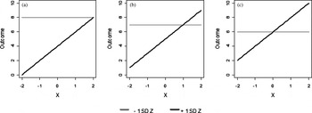
The distinction between the predictions of the diathesis–stress and the differential susceptibility models are illustrated in Figure 1.Footnote 1 The leftmost panel illustrates a prototypical case of diathesis–stress. According to this figure, individuals low on a moderator variable Z (e.g., difficult temperament) do not exhibit an association between a focal predictor X (e.g., maternal sensitivity) and an outcome variable Y (e.g., social competence). People who are high on the moderator variable (Z), however, exhibit a positive relation between maternal sensitivity (X) and social competence (Y). The rightmost panel of Figure 1 illustrates prototypical differential susceptibility predictions. In this example, there is again no association between X and Y (maternal sensitivity and social competence) among people who have low scores on the moderator variable Z. However, there is a positive association between X and Y among people with high scores on the moderator variable Z. In this particular situation, the two regression lines intersect near the middle of the distribution of maternal sensitivity. Thus, individuals with a difficult temperament are more well adjusted than others at high levels of parental sensitivity, but they are less well adjusted compared to others at low levels of parental sensitivity.
(a) Prototypical diathesis–stress and (c) differential susceptibility interaction plots based on X–Y simple slopes at ±1 SD from the mean of Z (moderator). (b) A visually ambiguous plot. Higher values on X (standardized) and Y (unstandardized) indicate positively valenced developmental inputs and outcomes, respectively. Higher values on Z represent higher levels of susceptibility/risk factor.

In a series of recent publications (e.g., Belsky et al., Reference Belsky, Bakermans-Kranenburg and van IJzendoorn2007; Belsky & Pluess, Reference Belsky and Pluess2009), Belsky and colleagues have developed criteria for establishing differential susceptibility, and in particular, distinguishing evidence for it from support for other models of development involving statistical moderation, most notably diathesis–stress accounts. These scholars note that making this determination includes, first, conducting a formal statistical test for a crossover (or, more formally, disordinal) interaction, and second, comparing the resultant plot with the prototypical ones displayed in Figure 1 (and distinguishing these from other kinds of interactions, including contrastive effects).Footnote 2
Evaluating one's data in light of these criteria can be accomplished in part by following the well-known recommendations of Aiken and West (Reference Aiken and West1991), which involve regressing the dependent measure of interest simultaneously on (centered) independent and moderator variables and their interaction (i.e., the product of the centered predictor and moderator variable). The regression model is

where X represents developmental experiences (e.g., parenting quality), Z represents the moderator variable (e.g., temperament), and Y represents the outcome variable (e.g., social competence). A significant interaction term (b 3) indicates that the association between X and Y varies as a function of Z, but it does not specify the form of the interaction. To better understand the form of the interaction it is valuable to plot the regression of Y on X at various levels of Z (e.g., 1 SD above and below the mean of Z). Traditionally, researchers have supplemented such plots by conducting a simple slopes analysis (e.g., Aiken & West, Reference Aiken and West1991, p. 78). Simple slopes analysis determines whether the association between the predictor and outcome is statistically significant (and estimates the magnitude and valence of that association) at relatively high or relatively low levels of the moderator (or both; again, by convention, at ±1 SD from the mean value of the moderator when Z is continuously distributed).Footnote 3
Developmental methodologists (e.g., Dearing & Hamilton, Reference Dearing and Hamilton2006) have recently begun advocating that, instead of conducting simple slopes analysis, in which significant interactions are probed at (for continuous variables) two arbitrarily specified levels of the moderator (i.e., ±1 SD), researchers should instead examine regions of significance (RoS). In the standard case, RoS, which can be computed using the Johnson–Neyman technique and online calculators that implement it (http://www.quantpsy.org; Preacher, Curran, & Bauer, Reference Preacher, Curran and Bauer2006), refer to the range of values of the moderator for which the independent and dependent variable are significantly associated (what we refer to here as the RoS on Z). The potential value of focusing on RoS on Z is that these regions highlight all possible values of Z for which there are significant regressions of Y on X, instead of probing only two possibilities (i.e., values of Z that are 1 SD above and below the mean).
Although we agree that the criteria described above for identifying evidence for differential susceptibility are essential,Footnote 4 implementing them is less than straightforward in ways that may not be fully appreciated by developmental psychologists interested in evaluating accounts of differential susceptibility. In light of this, we present four critiques of methods used to identify evidence for differential susceptibility in turn. Our goal in presenting these critiques is to highlight a set of standards by which to distinguish a differential susceptibility effect from (a) a diathesis–stress effect and (b) random data fluctuations. After presenting these critiques, we illustrate how to evaluate the merits of each critique using data from the NICHD SECCYD.
Critique 1: The Visual Inspection Critique
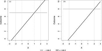
Much of the research conducted with a focus on examining differential susceptibility has involved simple visual inspection of the interaction plot for evidence of crossover (e.g., Bradley & Corwyn, Reference Bradley and Corwyn2008; Dopkins-Stright et al., Reference Dopkins-Stright, Cranley Gallagher and Kelley2008). There are two problems with this approach. First, all interactions would eventually cross over if extrapolated to a wide enough range of X. As such, it is essential that there is strong a priori agreement among researchers about what constitutes the research range of interest on the independent (X) variable across studies of differential susceptibility (Pedhazur, Reference Pedhazur1982, p. 461).Footnote 5 In other words, there must be consensus on what constitutes the normative range of the independent variable that should be probed. To clarify why this is so critical, consider Figure 2a. A researcher who bounded the range of interest at −1 and +1 SD from the mean (dotted vertical lines) on the independent variable would conclude based on visual inspection alone that these (simulated) data were consistent with a prototypical diathesis–stress model. In contrast, a researcher who bounded the range of interest at −2 and +2 SD from the mean (solid vertical lines) would interpret the very same data as evidence for differential susceptibility. Figure 2b shows that, given a broad enough sampling of the range of the independent variable (however rare some of those values are likely to be actually represented in the population), interactions probably best understood as evidence for diathesis–stress (i.e., using the ±2 SD boundaries, solid vertical lines) would resemble a function suggestive of differential susceptibility (i.e., using bounds of ±3 SD, dashed vertical lines).
An illustration that conclusions regarding the form of an interaction vary as a function of the range of interest on the X variable. Dashed and solid vertical lines denote investigator-specified choices about ranges of interest on X (see text).

The principal recommendation that follows from the analysis above is that the same range of interest must be interrogated across studies of differential susceptibility. It is often difficult to discern what range of interest was used by investigators who plot raw (even if centered) variables, rather than standardized ones, especially if researchers label the x axis of interaction figures with terms like “low” and “high” without further explanation, as is commonplace. As such, we endorse the recommended practice (Aiken & West, Reference Aiken and West1991) of probing interactions from −2 to +2 SD from the mean for the independent variable because, given a normally distributed variable, 2 SD below and above the mean covers over 95% of the sample.
Assuming that all investigators adopt the same range of interest on X, a second problem remains regarding how to objectively probe the interactions to determine whether they are more consistent with diathesis–stress or differential susceptibility models. The problem becomes clear in examining Figure 1b. It is almost certainly the case that, by simply eyeballing this plot, some observers would see this figure as consistent with evidence for differential susceptibility, whereas others would see it as suggestive of diathesis–stress (the simulated plot was designed to be ambiguous in this respect, but is fairly representative of actual interaction effects reported in the literature; see Dick et al., Reference Dick, Meyers, Latendresse, Creemers, Lansford and Pettit2011).
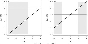
In order to counter this level of unacceptable subjectivity, Kochaska et al. (Reference Kochanska, Kim, Barry and Philibert2011) recently suggested that researchers follow the recommendations for probing interactions described in Dearing and Hamilton (Reference Dearing and Hamilton2006). Specifically, they endorsed the view that investigators identify what we refer to here as regions of significance on X (RoS on X), an approach that inverts the RoS on Z test to examine the values of X for which the moderator and outcome variable are significantly related. The benefit of conducting this analysis is that it provides a test of the statistical significance of the association between the moderator and the outcome at all values of X that fall within the range of interest.Footnote 6 If the association between the moderator and the outcome is significant at the low but not high end of X, there is evidence that the data support the diathesis–stress model (see Figure 3a in which, as is standard practice, regions of significance on X in gray are overlaid on a plot of an interaction depicted using simple slopes at −1 and +1 SD on a continuously distributed moderator variable). If the association between the moderator and the outcome is significant at both the low and high ends of the distribution of the independent variable within the normative range (i.e., ±2 SD), there is evidence of differential susceptibility (see Figure 3b; see Kochanska et al., Reference Kochanska, Kim, Barry and Philibert2011, for an early example of the implementation of the RoS on X test applied to the differential susceptibility hypothesis).
Regions of significance (RoS) on X for (a) diathesis–stress and (b) differential susceptibility models. Gray shaded area denotes regions where the two lines significantly differ.

Although there is emerging awareness of RoS on X analyses among differential susceptibility researchers (e.g., Belsky & Pluess, in press; Kochanska et al., Reference Kochanska, Kim, Barry and Philibert2011), visual inspection of interaction plots to identify evidence for differential susceptibility remains widespread in recent publications (e.g., Pluess & Belsky, Reference Pluess and Belsky2010). We recommend that researchers discontinue this practice. Moreover, when RoS on X analyses are used, it is crucial that the same range of interest is examined across all studies of differential susceptibility, which we recommend should be bracketed by ±2 SD from the mean of X.
Critique 1: Visually apparent differential susceptibility evidence in an interaction plot may not be statistically distinguishable from data generated by a diathesis–stress model, a problem that is compounded if different researchers choose to adopt different ranges of interest on the X variable under investigation.
Proposed Critical Test 1: Researchers should apply a Regions of Significance (RoS) on X test (Dearing & Hamilton, Reference Dearing and Hamilton2006; Kochanska et al., Reference Kochanska, Kim, Barry and Philibert2011) to demonstrate that Y (e.g., social competence) and Z (e.g., difficult temperament) are correlated both at the high and low ends of the distribution of X (e.g., maternal sensitivity) bounded by a conventional range of interest that is ±2 SD from the mean of X.
Critique 2: The Quantification Critique
Although the RoS on X analysis would appear to make differentiating between differential susceptibility and diathesis–stress more objective when faced with the ambiguity of, say, the plot depicted in Figure 1b, an underappreciated problem with this approach that flows from null hypothesis significance testing generally is that the test in not invariant to sample size (Cohen, Reference Cohen1988; Fraley & Marks, Reference Fraley, Marks, Robins, Fraley and Krueger2007). For example, in the relatively small sample size case it will be quite common to observe plots that would seem highly consistent with a differential susceptibility account (i.e., that look much like Figure 1c) but, due to low statistical power, might be interpreted (wrongly) as evidence for diathesis–stress.
What is potentially more concerning, however, is the problem that can emerge in a large N study. The problem in this empirical context is that even trivial evidence for a crossover interaction at the highest values of the predictor variable within the range of interest will eventually be detected as statistically significant as sample size increases. What this means is that, with enough N, any interaction that features some crossover at the high end of the predictor distribution—however trivial the magnitude of this difference—will be viewed through the prism of RoS on X testing as consistent with the differential susceptibility account. To be clear, large N designs are valuable because they allow theoretical parameters to be estimated with high precision. In the context of null hypothesis significance testing, however, they can be abused to highlight trivial differences that may actually have no practical or theoretical significance.
Two novel metrics for quantifying evidence for differential susceptibility
To avoid sample size driving the interpretation of interaction effects, we offer here two novel solutions to distinguish between differential susceptibility and diathesis–stress that can be used to supplement the RoS on X approach (particularly in the large N empirical context). Both proposed metrics are unitless, and they are also independent of sample size. The first of these involves creating an indexFootnote 7 of the degree to which an interaction conforms to the prototypic one for differential susceptibility. One straightforward way to accomplish this is to measure the proportion of the total area represented in the relevant figures (see Figure 4a and b) uniquely attributable to differential susceptibility. We refer to this proposed metric, b/(b + w), as the proportion of interaction (PoI) index.
Proportion of the interaction (PoI) for (a) diathesis–stress and (b) differential susceptibility models. w, worse; b, better.

Both the differential susceptibility and diathesis–stress accounts anticipate the area labeled w (i.e., for worse) in Figure 4a and b. That is, both the differential susceptibility and diathesis–stress accounts require that individuals who experience poor developmental inputs (i.e., low levels of maternal sensitivity) and who are otherwise at risk (i.e., due to difficult temperament) should fare less well than individuals with only one of those risk factors. What the differential susceptibility hypothesis uniquely predicts, however, is that it will also be the case that the interaction effect will be driven by the area of the plotted interaction that we label b (for better) in Figure 4b, which is evidence that (for reasons previously explained) individuals who have the same putative risk factor (difficult temperament in this example) actually should be expected to be more successful than their temperamentally easy counterparts given positive developmental inputs. Furthermore, prototypic differential susceptibility and diathesis–stress plots allow us to place a point prediction on the expected values of the areas of w and b. Specifically, w should be equal to 100% in the prototypic case of diathesis–stress (i.e., b/[b + w] should equal 0.00), whereas w and b should both equal 50% in the prototypic case of differential susceptibility (i.e., b/[b + w] should equal 0.50).Footnote 8 (This assumes that, once X is standardized, a value of zero anchors the true mean for the construct of interest tapped by the measure of X; see footnote 5 and the Discussion Section for elaboration on this important issue.Footnote 9
One of the major strengths of the PoI metric for quantifying evidence for differential susceptibility (and diathesis–stress) is that, unlike the p values used in RoS tests, PoI is not an explicit function of sample size. However, like regions of significance, it will produce different results if different researchers define their ranges of interest using different criteria (e.g., the results for ±1 SD differ from those produced using ±2 SD). Thus, we recommend that researchers consistently probe ±2 SD on the X variable so the PoI metric requires no additional assumptions beyond those already in use when plotting interactions generally.
Critique 2: There is no standard index for the quantification of differential susceptibility (or diathesis–stress) effects. Thus, inferences of diathesis–stress versus differential susceptibility are driven largely by statistical significance testing and sample size using the RoS on X test or, more commonly, visual inspection of the interaction plot.
Proposed Critical Test 2a: In addition to RoS on X testing, researchers should apply a diathesis–stress/differential susceptibility index, PoI, to help distinguish differential susceptibility evidence from diathesis–stress evidence. PoI values close to 0.50 suggest strong evidence for differential susceptibility. Values closer to 0.00 suggest strong evidence for diathesis–stress.
An alternative to the PoI index, which is one that avoids the need to specify a range of interest altogether, is to estimate the proportion of the population that is differentially affected by the moderator: the proportion affected (PA) index. The logic of this approach is relatively straightforward. The goal is to identify first the value of X at which the regression lines cross over. The crossover value is located at

where b 2 is the semipartial main effect of Z on Y from Equation 1, and b 3 is the interaction effect from Equation 1.
The crossover point is the threshold at which the association between Z and Y changes meaning as a function of X. Thus, the number of people who are differentially affected (i.e., the proportion affected or the PA index) can be computed by sorting the dataset with respect to X and calculating the proportion of cases that fall above the crossover point. If the number/proportion of people above the crossover exceeds a prespecified threshold, then one concludes in favor of differential susceptibility. If the proportion of people above the crossover is less than that threshold, one concludes in favor of diathesis–stress.
The potential value of the PA index is that it offers a pragmatic way of evaluating evidence for differential susceptibility. Namely, it could be argued that, even if there is evidence for differential susceptibility according to other criteria (e.g., RoS on X tests), the model is of limited use if only a small number of individuals experience the theorized benefits. What threshold should be used? Typically, the PA index will range from around 0.50 (indicating strong evidence for differential susceptibility) to 0.00 (in the clear case of diathesis–stress). However, in the interest of establishing default conventions, we suggest that if only 16% of cases fall above the point at which the regression lines intersect, investigators should begin to question whether their data are consistent with differential susceptibility theory; when less than 2% of cases fall above the point at which the regression lines intersect, such evidence should definitely not be interpreted as evidence for differential susceptibility.Footnote 10 Although the selection of any threshold is necessarily arbitrary, our justification for these particular thresholds is that approximately 16% and 2% of cases will fall 1 and 2 SD, respectively, above the mean on a normal distribution.
Proposed Critical Test 2b: Researchers should estimate the percentage of the population above the crossover point. Larger percentages suggest stronger evidence for differential susceptibility relative to diathesis–stress.
Critique 3: The Type I Error Critique
Capitalizing on chance?
When testing a differential susceptibility hypothesis, it is not uncommon for researchers to have access to data on many different variables that might alternatively be used to operationalize X, Z, and Y. In such instances, it can be possible to conduct many, separate tests for differential susceptibility. For instance, if there are 2 X variables (e.g., two different measures of parental sensitivity), 2 Z variables (e.g., two different measures of temperament), and 15 Y variables (e.g., three different outcome measures, Y, each taken at five different points in time), then a researcher might ostensibly conduct 2 × 2 × 15 = 60 separate tests of the differential susceptibility effect. With so many tests, the probability of committing a Type I error (i.e., concluding the effect exists when, in fact, it does not) for any single test of differential susceptibility (or diathesis–stress) is quite high. For example, at a nominal a level of 0.05 (5% Type I error rate) for each test, the familywise Type I error rate for falsely rejecting the null hypothesis for any one of 12 independent significance tests is 1 – (1 – 0.05)12 = 46% (Sidak, Reference Sidak1967), which much larger than 5%. Because the significance tests for 60 different operationalizations of the interaction effect (described above) involves many nonindependent tests, it can be complicated to estimate the exact overall Type I error rate across multiple comparisons (see Benjamini & Yekutieli, Reference Benjamini and Yekutieli2001). Nevertheless, we note that Type I error rate is extremely high in traditional tests of differential susceptibility and diathesis–stress. This issue is potentially exacerbated in developmental tests of differential susceptibility and diathesis–stress, because the same outcome variable is often measured longitudinally—creating a strong possibility that differential susceptibility may appear at one point in time, but not at others.
True developmental sensitive periods?
One issue that applies to the evidence for differential susceptibility and diathesis–stress is that of the relative inattention in this literature to date on development itself (but see Belsky & Pluess, in press). In a typical study in this literature, caregiving experiences (e.g., maternal sensitivity) and a putative plasticity agent (e.g., difficult temperament) are measured at some point early in the life course and the correlates of those experiences are assessed at another point later in time. The caveats we have thus far offered aside, if the predictive significance of those early experiences are significantly moderated by the plasticity factor in a manner resembling Figure 1c, researchers conclude that they have documented evidence for differential susceptibility (conclusions that as noted earlier have often not involved the application of the RoS on X test; see, e.g., Pluess & Belsky, Reference Pluess and Belsky2010).
However, what may not be obvious in such analyses is that such effects may either fade or endure over time (for a broader discussion of this problem, see Fraley, Roisman, & Haltigan, in press). What seems especially problematic is that even when multiple assessments of a given dependent variable across time and informant are available (e.g., in longitudinal studies such as the NICHD SECCYD), most studies of differential susceptibility tend to be focused on the way the predictive significance of early caregiving experiences is moderated by difficult temperament in relation to a set of outcomes all of which are assessed at a single assessment, sometimes by the same informant (but see Belsky & Pluess, in press; Pluess & Belsky, Reference Pluess and Belsky2009, Reference Pluess and Belsky2010). Dopkins-Stright et al. (Reference Dopkins-Stright, Cranley Gallagher and Kelley2008), for example, found evidence that individuals with difficult temperament in the NICHD SECCYD were more susceptible to the effects of early maternal sensitivity in the sense that they benefitted more from high quality caregiving and were disproportionately negatively affected by insensitive caregiving than those low on temperamental difficulty. However, all of the outcomes examined in that report were assessed at a single assessment (Grade 1) by the same informant (i.e., the participants' teachers).
What might be discovered by examining the same outcome variables available on the SECCYD in multiple assessments across time and informant through midadolescence? In advance of examining this question empirically, it is impossible to know. However, it is possible that the evidence for differential susceptibility might have been transient. One way to examine this empirically is to examine how the interaction effect varies as a function of when the outcome variable in question was assessed. Second, assuming evidence for moderation is consistent over time, the potentially dynamic shape of significant interaction effects can be evaluated by plotting the PoI or PA metrics described above as a function of the age at which the outcome was assessed. For example, if the PoI metric tends to be close to a value of 0.50 and relatively stable over time, this would provide compelling evidence that early temperament is a marker of differential susceptibility to early caregiving experiences, in a way that is reflected in an enduring manner in developmental adaptation. The presentation of all available dependent data in longitudinal studies also helps rule out the possibility that evidence for differential susceptibility or diathesis–stress at any given assessment point is merely Type I error.
Moreover, two methodological protections against developmental Type I error (i.e., finding statistically significant effects for an outcome measured at one point in time, but not for outcomes measured at others) are also available. First, when the researcher is interested in a true developmental sensitive period (i.e., a true effect that obtains at some time points but not others) then it may be valuable to apply a more conservative a level (e.g., Dunn, Reference Dunn1961; Sidak, Reference Sidak1967) to rule out the possibility that this particular time period appears significant by chance alone. We recommend a sequential Bonferroni-type procedure (Benjamini & Hochberg, Reference Benjamini and Hochberg1995; Simes, Reference Simes1986; see Appendix A), which controls the false discovery rate but can be considerably more powerful than the traditional Bonferroni procedure. Second, when the researcher is interested in differential susceptibility in general (at the potential cost of ignoring any developmental patterns over time), then we recommend aggregating outcome variables across time, via a multilevel model (intercepts as outcomes model; see Pluess & Belsky, Reference Pluess and Belsky2010; Raudenbush & Bryk, Reference Raudenbush and Bryk2002).
Critique 3: Differential susceptibility effects that appear in only a few out of many statistical tests attempted are likely the result of Type I error (i.e., a high probability of getting at least one false positive result when many tests are conducted).
Proposed Critical Test 3a: Researchers should apply multilevel models to determine overall differential susceptibility for outcomes, averaged across the entire developmental course (i.e., using intercepts as outcomes models).
Proposed Critical Test 3b: If an apparent differential susceptibility effect emerges at some points in time but not at others, then researchers should apply a more conservative procedure for Type I error control (Benjamini & Hochberg, Reference Benjamini and Hochberg1995).
At this point, an important caveat is in order concerning Critical Test 3b. That is, one possible reason for an interaction effect to emerge at one point in time but not at others could be the existence of interindividual differences in intraindividual change (i.e., linear and quadratic slope effects over time; Baltes, Reese, & Nesselroade, Reference Baltes, Reese and Nesselroade1977; Raudenbush & Bryk, Reference Raudenbush and Bryk2002). As an example of this, if the Sensitivity × Temperament interaction effect gets systematically stronger at later time points, this might reflect a positive association between the interaction term and the linear slope of the outcome variable. As such, in addition to Critical Test 3b, researchers should also inspect whether the interaction terms, PoI, and PA indices follow a systematic pattern (e.g., monotonically rising or declining).
Critique 4: The Nonlinearity Critique
Finally, we note that apparent differential susceptibility effects might logically be an artifact of imposing a linear model on a plausibly nonlinear phenomenon. This is illustrated in Figure 5. In this figure we observe a diathesis–stress effect in which there is a nonlinear X–Y relationship. Suppose for the sake of the argument that there are diminishing returns to parental sensitivity (X), such that children benefit more from a unit increase in caregiver sensitivity when sensitivity is scarce than when sensitivity is more available (i.e., the X–Y relationship is stronger at lower levels of X). In addition, we might reasonably suppose, as is consistent with the diathesis–stress perspective, that any nonlinear X–Y effect (where low parental sensitivity becomes increasingly harmful when sensitivity is already scarce) is especially likely to emerge among children with difficult temperaments (i.e., high Z).
Nonlinear relations masquerading as differential susceptibility. The solid lines represent predictions from a nonlinear model. The dashed lines represent predictions from a linear model. (Note the linear and nonlinear lines for +1 SD Z overlap.)

The point of Figure 5 is that, if such a nonlinear phenomenon existed, imposing a linear predictor model on the data (as is standard; see the dashed lines in Figure 5) might lead researchers to observe a differential susceptibility effect that does not really exist. To test this possibility, it would be necessary to estimate differential susceptibility while demonstrating the absence of nonlinear terms X 2 and ZX 2 (see Cortina, Reference Cortina1993).
Critique 4: Apparent differential susceptibility effects can be an artifact of imposing a linear predictor model on a nonlinear diathesis–stress phenomenon.
Proposed Critical Test 4: When testing differential susceptibility, researchers should estimate an additional model that includes X 2 and ZX 2. The results of this model must show that neither X 2, ZX 2, nor the combination of both X 2 and ZX 2 together is statistically significant. If one of these nonlinear X 2 terms is significant, then the researcher must demonstrate that the XZ interaction term remains statistically significant even after controlling for the nonlinear terms.
An Empirical Example in the NICHD SECCYD
To provide a demonstration of how the substantive conclusions in this area of research are potentially subject to change as a function of the critiques provided above, in the remainder of this report we revisit the literature on difficult temperament as a susceptibility factor in relation to early maternal sensitivity using data drawn from the NICHD SECCYD. To our knowledge, three published studies have highlighted the role of early difficult temperament (assessed using a maternal report questionnaire at 1 and/or 6 months in all three studies) in amplifying the predictive significance of early observations of maternal sensitivity, for better and for worse, in the SECCYD dataset. Dopkins-Stright et al. (Reference Dopkins-Stright, Cranley Gallagher and Kelley2008) focused on academic competence, social skills, and relationships with teachers and peers measured during first grade. Bradley and Corwyn (Reference Bradley and Corwyn2008) examined externalizing problems, also assessed by teachers in first grade. Finally, and most recently, Pluess and Belsky (Reference Pluess and Belsky2010) focused on assessments of cognitive–academic and social skills. Data presented in each of these studies were interpreted as supporting the differential susceptibility model over the diathesis–stress account, although none used the RoS on X test as a basis for that conclusion (but see Belsky & Pluess, in press).
The present study revisits and extends these recent reports, as well as our own analyses of the NICHD SECCYD (Fraley et al., Reference Fraley, Roisman and Haltiganin press; Haltigan, Roisman, & Fraley, in press) in which we have found that early observed maternal sensitivity assessed through 36 months is associated in an enduring manner with academic skills (teacher reported through Grade 6 and based on objective assessments through age 15), social competence (mother reported through age 15 and teacher reported through Grade 6), and teacher-reported symptoms of psychopathology (through Grade 6). (The predictive significance of early maternal sensitivity for mother reports of symptomatology was demonstrated in this work to fade over time in the SECCYD through age 15; that is, early sensitivity was an increasingly weaker predictor of mother reports of symptomatology as children in the cohort aged; Haltigan et al., in press).
More specifically, we apply the methods described above to examine whether early difficult temperament reliably moderates the association between early observed sensitivity and developmental adaptation over time within and across the key domains of (mal)adaptation described above in the SECCYD. Along the way, we seek to assess whether the differential susceptibility hypothesis can survive the tests we articulated above. We present the results of RoS on Z and RoS on X tests, novel differential susceptibility/diathesis–stress indices PoI (b/[b + w]) and PA, significance tests with conservative critical α levels and multilevel intercepts as outcomes models, and nonlinear predictor models, to quantify the evidence for differential susceptibility versus diathesis–stress. We will consider if and how such metrics change as a function of when the dependent measures were assessed in order to explore the developmental course of these moderated associations. In addition to providing new data on the SECCYD cohort (i.e., through age 15, where applicable), this analysis provides a representative test of the differential susceptibility and diathesis–stress hypotheses in the SECCYD in relation to early maternal sensitivity, early difficult temperament, and a fairly comprehensive range of markers of developmental (mal)adaptation.
Method
Participants
Families were recruited for the NICHD SECCYD in 1991 from hospitals located in or near Little Rock, Arkansas; Orange County, California; Lawrence, Kansas; Boston, Massachusetts; Pittsburgh, Pennsylvania; Philadelphia, Pennsylvania; Charlottesville, Virginia; Seattle, Washington; Morganton, North Carolina; and Madison, Wisconsin. During selected 24-hr sampling periods, 8,986 women who gave birth were screened, 5,416 of whom met the eligibility criteria for the study. Families were excluded if (a) the mother was younger than 18 years of age, (b) the family planned to move, (c) there was a multiple birth, (d) the infant had a known disability or remained in the hospital more than 7 days, (e) the mother acknowledged substance abuse, (f) the mother did not speak English, and/or (g) the mother lived more than 1 hr from the laboratory site or in an extremely unsafe neighborhood, as determined by local police. From that group, 1,364 families became study participants upon completing an interview when their infants were 1 month old. Details about recruitment and selection procedures are available in prior publications from the study (see NICHD ECCRN, 2005) and the Web (http://secc.rti.org). Note that, although large, demographically diverse, and methodologically rich, the SECCYD was not designed to be a nationally representative study.
Analysis sample
The analysis sample for this study included the 1,306 children (52% males) for whom any observational data were collected at ages 6, 15, 24, and/or 36 months that focused on the quality of the maternal caregiving they experienced in the first 3 years of life. In terms of race/ethnicity, 77% of the children from the analysis sample for this study were White/non-Hispanic. Note that for all modeling analyses described below, multiple imputation (m = 20 imputations) was used with raw case-level analytic data as input, to produce less biased and more efficient and consistent parameter estimates than techniques such as pairwise or listwise deletion for longitudinal missing data (Newman, Reference Newman2003; Rubin, Reference Rubin1987; Schafer, Reference Schafer1997; Schafer & Graham, Reference Schafer and Graham2002). These analyses mirror the multiple imputation approach used by Pluess and Belsky (Reference Pluess and Belsky2010). Further, we followed Collins, Schafer, and Kam's (Reference Collins, Schafer and Kam2001) inclusive strategy of using all study variables in the imputation model, rather than just a subset of variables (see Graham, Reference Graham2003), as well as Enders' (Reference Enders2010) and Graham's (Reference Graham2009) recommendation to incorporate the interaction term into the imputation model when testing moderated effects, to avoid a known problem where the linear imputation model biases interaction effects toward zero. Predictor variables were standardized using the expectation–maximization algorithm (maximum likelihood) means and standard deviations, as advised by Enders (Reference Enders2010). Moderation analyses were performed in SAS 9.1 Proc MI, Proc Reg, and Proc Mixed; syntax files are available from the second author. RoS on Z, RoS on X, PoI, the crossover point for the interaction, and the PA indexes were generated using a Web-based program developed by the third author. The application is freely available at http://www.yourpersonality.net/interaction/ and can also be used to generate and explore interaction plots and to conduct simple slope tests.
Measures
Measures are presented in four sets corresponding to their function in the analytic plan, as follows: (a) variables used to create a composite measure of the observed quality of participants' experience with caregivers in the first 3 years of life; (b) measures of social competence, as assessed by primary caregivers and teachers through the latest assessment for which these data were available (mother: age 15; teacher: Grade 6); (c) measures of academic skills, as rated by teachers and assessed using standardized tests through the latest assessment for which relevant data were acquired (teacher reports: Grade 6; standardized assessments: age 15); and (d) reports of total problem behavior, as assessed by primary caregivers and teachers from the first through the latest assessment for which these data were available (mother: age 15; teacher: Grade 6). In all cases we selected variables that were measured multiple times by multiple reporters using standard assessment tools.
Early maternal sensitivity
Mother–child interactions were videotaped during 15-min semistructured tasks at 6, 15, 24, and 36 months. A number of scales were used to rate the mothers' behavior from these videotapes. More specifically, at 6 months, mothers and children were instructed to play together, first with toys available in the home (or none at all) and then with a standard set of toys. At 15, 24, and 36 months, mothers were asked to show their children age-appropriate toys in three containers in a set order. As in prior studies of this sample (e.g., NICHD ECCRN, 2001), observations of maternal sensitivity from the first 3 years of life (6, 15, 24, and 36 months) were standardized and averaged to create a composite of the observed early sensitivity. Note that at 6, 15, and 24 months, the a priori maternal sensitivity composites were constructed by summing ratings for sensitivity to nondistress, positive regard, and intrusiveness (reversed). At 36 months the supportive presence, respect for autonomy, and hostility (reversed) scales were composited (as reported in NICHD ECCRN, 2001, internal consistencies of composites were 0.75, 0.70, 0.79, and 0.78 for the 6, 15, 24, and 36 month composites, respectively, and intercoder reliabilities on scales >0.80). Within age composites showed stability over time (rs range = .30–48; standardized α for composite measure = 0.73).
Early temperament
At the 6-month visits, mothers completed the Carey and McDevitt (Reference Carey and McDevitt1978) Infant Temperament Questionnaire, which contained 38 items rated on a 6-point scale. The composite total score, with higher scores reflecting a more irritable and difficult child, had adequate reliability (α = 0.81). We selected the 6-month Infant Temperament Questionnaire data in the current analyses rather than a composite of the 1- and 6-month data as has been done in at least one prior investigation of differential susceptibility (i.e., Bradley & Corwyn, Reference Bradley and Corwyn2008) based on both psychometric considerations: the 1-month temperament composite possessed only modest reliability relative to the 6-month temperament composite (α = 0.67 vs. α = 0.81, respectively; Roisman et al., Reference Roisman, Monahan, Campbell, Steinberg and Cauffman2010) and the 1- and 6-month temperament composites are only modestly correlated (r = .32; Roisman, Susman, et al., Reference Roisman, Susman, Barnett-Walker, Booth-LaForce, Owen and Belsky2009). We also selected it because Pluess and Belsky (Reference Pluess and Belsky2010) explicitly noted in a prior examination of the 1- and 6-month temperament data with respect to differential susceptibility that “temperament scores at 6 months were not averaged with a similar measure at 1 month because preliminary hierarchical linear model analyses showed that the 6-month measure yielded stronger interaction effects than the average of the two measurement occasions” (p. 381).
Total problem symptomatology
Symptoms of psychopathology from childhood to adolescence were assessed with the total problem scale of the Child Behavior Checklist (CBCL) obtained using the parent and Teacher Report Form (TRF) versions (Achenbach, Reference Achenbach1991; Achenbach & Edelbrock, Reference Achenbach and Edelbrock1986; Achenbach, Edelbrock, & Howell, Reference Achenbach, Edelbrock and Howell1987). We used T scores. In the current study, maternal reports on the CBCL were used from the following assessment points: a mean composite of the 24- and 36-month CBCL (r = .73; p < .01); 54 months; kindergarten; Grades 1, 3, 4, 5, and 6; and age 15. Teacher reports were used from the following assessment points: kindergarten and Grades 1, 2, 3, 4, 5, and 6. The total problem behavior scale showed adequate reliability across time and had a coefficient α averaging 0.93 for maternal reports and 0.96 for teacher reports across all assessments.
Social competence
Mothers completed the 38-item Social Skills Questionnaire from the Social Skills Rating System (SSRS; Gresham & Elliott, Reference Gresham and Elliott1990) when children were age 54 months and in kindergarten; Grades 1, 3, 4, 5, and 6; and at age 15, indexing general social competence with adults and other children. To obtain a standardized measure of total social skills, an a priori scale was created by summing all items that index social competence with other children, with higher scores indicating more socially skilled children (αs range = 0.87–0.91; M = 0.89). In a parallel fashion, teachers completed the 30-item school version of the Social Skills Questionnaire from the SSRS when children were in kindergarten as well as Grades 1, 2, 3, 4, 5, and 6. As with the mother reports, a standardized total social skills scale was created by summing items indexing social competence (αs range = 0.93–0.94; M = 0.94).
Academic skills
Teachers also used the SSRS to rate participants' academic skills when children were in kindergarten and Grades 1, 2, 3, 4, and 5 (αs range = 0.94–0.95; M = 0.95). For use in this study, an a priori, standardized academic competence scale was created by summing items indexing academic success. In addition, in order to examine a relatively objective assessment of academic skills we used Woodcock–Johnson Psycho-Educational Battery—Revised (WJ-R; Woodcock, Reference Woodcock1990; Woodcock & Johnson, Reference Woodcock and Johnson1989) scores at 54 months; Grades 1, 3, and 5; and age 15. Note that for the WJ-R, a slightly different subset of scales was used at each assessment point. For purposes of this analysis, we averaged the W (standard) scores for all available subscales at each time point (within time αs range = 0.81–0.91; M = 0.87).
Control variables
Although there are a large number of potential control variables to consider, we selected four that we have examined in previous research (e.g., Fraley et al., Reference Fraley, Roisman and Haltiganin press; Roisman, Booth-LaForce, et al., Reference Roisman, Booth-LaForce, Cauffman and Spieker2009; Roisman, Susman, et al., Reference Roisman, Susman, Barnett-Walker, Booth-LaForce, Owen and Belsky2009) and which are known to correlate with maternal sensitivity and the outcomes examined in this report: child gender, child ethnicity, maternal education, and family income to needs. Child gender was coded in a binary fashion (1 = female, 0 = male). Because the majority of the children in the sample were White/non-Hispanic, we created a binary variable to represent ethnicity (1 = White/non-Hispanic, 0 = otherwise). Maternal education was coded on an ordered metric representing the number of years of education/highest degree. Family financial resources were operationalized as an income to needs ratio. Income to needs was computed separately within each of four assessment waves (6, 15, 24, and 36 months) and averaged to create a mean income to needs index for early childhood. Each of these variables was entered into all analyses reported below.
Results
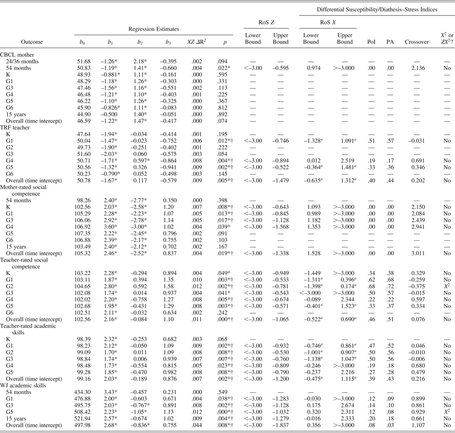
Results of the tests of differential susceptibility and diathesis stress are presented in Table 1. For each outcome variable (e.g., mother-reported CBCL, teacher-rated social competence), we first report the results for a regression model at each point in time (54 months, kindergarten, Grade 1, etc.), followed by the overall (mean) effect from an intercepts as outcomes multilevel model (i.e., a random intercepts model in which the intercept [average over time] of the outcome is treated as the dependent variable). These results in Table 1 show (a) whether the Parental Sensitivity × Difficult Temperament interaction effect is statistically significant; (b) whether the RoS on parental sensitivity (RoS on X) is within the bounds of −2 to +2 SD (Critical Test 1); (c) how large the differential susceptibility/diathesis–stress indices are (PoI and PA; Critical Tests 2a and 2b); (d) whether the effects emerge across the entire developmental course, on average (Critical Test 3a, intercepts as outcomes); (e) whether the effect observed at a single point in time is likely due to familywise Type I error (Critical Test 3b; Benjamini & Hochberg test); and (f) whether X 2 and ZX 2 nonlinear terms are statistically significant, and, if so, whether the XZ interaction term remains statistically significant in the model with significant nonlinear predictor terms (Critical Test 4). The results of these diathesis–stress/differential susceptibility tests are reported below, organized with respect to the outcome variables.
Regression estimates and differential susceptibility/diathesis–stress indices by outcome domain over time in the NICHD Study of Early Child Care and Youth Development
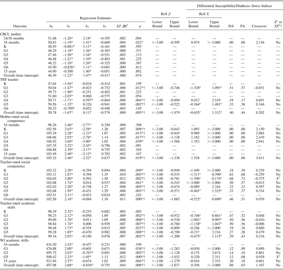
Note: RoS, regions of significance; PoI, proportion of interaction; PA, proportion affected; CBCL, Child Behavior Checklist; TRF, Teacher Report Form; K, kindergarten assessment; G1–G6, Grade 1–Grade 6 assessments; 15 years, 15-year-old assessment; WJ, Woodcock–Johnson. The regression equation Y = b 0 + b 1X + b 2Z + b 3XZ, where X is parental sensitivity and Z is difficult temperament (control variables not reported); RoS Z refers to the RoS with respect to temperament (Z). Specifically, the upper (lower) bound represents the value of temperament (standardized) above (below) which the regression of outcome on early sensitivity is statistically significant. RoS X refers to the RoS with respect to early sensitivity. Specifically, the upper (lower) bound represents the value of X (early sensitivity, standardized) above (below) which the regression of outcome on temperament is statistically significant. PoI falls above the cross-over point for the regressions. Cross-over represents the value of X (early sensitivity, standardized) at which the regression lines intersect. PA is the proportion of participants who had early sensitivity scores that fell above the crossover point. X 2 or ZX 2 denotes whether X 2, ZX 2, or the set of both nonlinear terms together was statistically significant in the equation Y = b 0 + b 1X + b 2Z + b 3XZ + b 3XZ + b 4X 2 + b 5ZX 2. Overall represents the average effect across all assessment waves, estimated from an intercepts as outcomes multilevel model centered at fifth grade (Pluess & Belsky, Reference Pluess and Belsky2010). The XZ ΔR 2 for the intercepts as outcomes model was estimated as 1 – (intercept variance with predictor/intercept variance without predictor).
aOutcomes for which both the lower and upper regions of significance with respect to early sensitivity (RoS X) fell within ±2 SD of the mean of early sensitivity.
*p < .05.
†False discovery rate p < .05 (controlling Type I error across multiple tests; Benjamini & Hochberg, Reference Benjamini and Hochberg1995).
Maternal reports of total problems
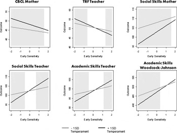
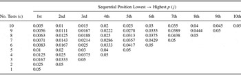
Regarding the possibility of differential susceptibility and diathesis stress effects for mother-reported CBCL, we see in Table 1 that the only statistically significant Parental Sensitivity × Difficult Temperament interaction effect appears when the outcome variable was measured at 54 months of age. The upper-bound RoS (RoS on X) for this effect appears above 2 SD, suggesting that this effect fails Critical Test 1 for differential susceptibility. Both the PoI and the PA are equal to 0.00, suggesting the observed interaction effect also fails Critical Tests 2a and 2b for differential susceptibility. Regarding Critical Test 3a, we see no statistically significant interaction effect for overall mother-reported CBCL using the intercepts as outcomes model (b 3 = −0.417; p = .074). Nevertheless, there was still a possibility that the interaction might reflect a true period of developmental sensitivity that emerges uniquely at 54 months of age. To test this, we used Critical Test 3b to calculate a conservative alpha level (critical p value) to control for the overall false discovery rate (Type I error) across multiple tests (see Appendix A for description of sequential Bonferroni procedure; Benjamini & Hochberg, Reference Benjamini and Hochberg1995). Noting that nine separate tests of the interaction effect were conducted for mother-rated CBCL, across nine waves of assessment (24 and 36 months; 54 months; kindergarten; Grades 1, 3, 4, 5, and 6; and 15 years), then because only one of these nine p values was below .05, the alpha level for the Benjamini and Hochberg (Reference Benjamini and Hochberg1995) sequential Bonferroni test would be .05 × (1/9 tests) = 0.0056 (see Appendix A). Because the observed p value at 54 months was p = .022 > .0056, we conclude that the observed interaction effect at 54 months fails Critical Test 3b. Last, in terms of the nonlinearity test (Critical Test 4), we find that neither X 2, ZX 2, nor the change in R 2 for the set of X 2 and ZX 2 together was statistically significant. In sum, the Parental Sensitivity × Difficult Temperament interaction effect on Mother CBCL failed Critical Tests 1, 2, and 3 for differential susceptibility and passed Critical Test 4 (i.e., lack of nonlinearity). The form of the overall interaction effect is depicted in Figure 6, first panel (labeled CBCL Mother), where we see that there is no suggestion of differential susceptibility for this outcome variable within 2 SD of the mean of X. Instead, Mother CBCL results seem more consistent with either diathesis–stress (note in Figure 6 that the RoS on X is shaded for low X only [i.e., high and low difficult temperament only differ at low levels of X, not at high levels of X]) or, perhaps more likely, any apparent interaction effect is due to Type I error.
Empirical results for each of the six outcome domains (overall effects, i.e., time intercept), with regions of significance on X tests (gray) superimposed on simple slopes (±1 SD on difficult temperament; Z = difficult temperament). Note that all interactions are statistically significant, except mother-reported total problems on the CBCL, which is included here only for purposes of comparison. CBCL, Child Behavior Checklist; TRF, Teacher Report Form.

Teacher reports of total problems
Next, for the outcome variable teacher-reported total problems (TRF teacher), there is a statistically significant early Sensitivity × Temperament interaction at Grades 1, 4, and 5, as well as a significant overall effect (averaged over time). The RoS on X test suggests significant differences between high and low Z (temperament) within the range from −2 to +2 SD on X (sensitivity) at Grade 1, Grade 5, and overall (passing Critical Test 1). In contrast at Grade 4, the upper bound for RoS on X was above +2 SD, meaning that temperament did not become a significant predictor until X (sensitivity) exceeded 2.519 SD above the mean (failing Critical Test 1). Regarding the magnitude of the differential susceptibility effect, PoI indices were uniformly above 18%, and PA was uniformly above 16% (passing Critical Tests 2a and 2b). Critical Test 3a was also passed for TRF Teacher, given that the intercepts as outcomes overall effect was significant and consistent with differential susceptibility. For Critical Test 3b (familywise Type I error), there were seven significance tests conducted and three p values less than .05 (p = .002, .004, and .012). Because the third largest p value .012 < .0214 (see Appendix A), then Grade 1, Grade 4, and Grade 5 effects remain statistically significant beyond chance alone. Finally, X 2, ZX 2, and the change in R 2 for X 2 and ZX 2 together were not statistically significant (passing Critical Test 4).
To summarize, differential susceptibility appears to be supported according to all critical tests at Grade 1, Grade 5, and in the overall (mean across time) effect. In the plot of the overall interaction in Figure 6, second panel (TRF teacher), we see shaded regions of significance (RoS on X) at both the high and low ends of X (Critical Test 1 for differential susceptibility). In other words, difficult temperament both (a) increases teacher-reported problems at low levels of sensitivity and (b) decreases teacher-reported problems at high levels of sensitivity. The data on teacher-reported problems clears all four hurdles for demonstrating differential susceptibility.
Maternal reports of social competence
For mother-rated social competence, the RoS on X test (Critical Test 1) fails under all conditions, because high and low temperament (Z) do not differ at high levels of X (+2 SD above the mean of parental sensitivity; see Figure 6, panel 3, Social Skills Mother). Consistent with this lack of evidence for differential susceptibility at high X, both PoI and PA are 0.00 for all conditions (Critical Tests 2a and 2b). The overall time intercept shows a significant interaction (Critical Test 3a), and this overall effect survives the conservative familywise Type I error test (Critical Test 3b); note that for the overall (time intercept) effects, we are testing six overall time intercept effects in Table 1, mother-rated social competence exhibits the fifth largest p value (p = .019), and this p value < .0417 (see Appendix A). There is no evidence of nonlinearity effects (passing Critical Test 4). To recap, mother-rated social competence seems consistent with a diathesis–stress account, rather than a differential susceptibility account. Regarding the chance that these observed interaction effects are due to familywise Type I error, note that three of these significant interaction effects pass the Benjamini–Hochberg test (see Appendix A, eight tests, third lowest p value = .017 < .0188), supporting the interaction at kindergarten, Grade 1, and Grade 3.
Teacher reports of social competence
For teacher-rated social competence, six out of seven assessment waves exhibited statistically significant interactions, and three of these (Grades 1, 2, and 5) passed the RoS on X test (Critical Test 1; temperament has significant effects in two different directions, within the range of +2 to −2 SD on early sensitivity). PoI and PA effect size indices were also large (uniformly above 21%, and above 50% in Grades 1, 2, and 3; passing Critical Test 2). The overall (time intercept) effect was significant (passing Critical Test 3a), and four of the seven waves were statistically significant beyond the familywise false discovery (Type I error) rate (passing Critical Test 3b). Only one assessment wave showed evidence of nonlinearity (X 2 effect was statistically significant at Grade 2), but the XZ interaction effect remained statistically significant after controlling both X 2 and ZX 2 (passing Critical Test 4). In total, teacher-rated social competence passes all four critical tests and shows strong evidence of differential susceptibility. Figure 6 corroborates this conclusion.
Teacher reports of academic skills
Teacher-rated academic skills (a) passed Critical Test 1 (RoS on X) at Grades 1, 2, 3, and overall, (b) passed Critical Tests 2a and 2b at all time points (PoI always >18% and PA always >17%), (c) passed Critical Test 3a (overall time intercept), (d) passed Critical Test 3b (familywise Type I error) at five out of six assessment waves, and (e) exhibited no nonlinearity. Teacher-rated academic skills reveal strong evidence of differential susceptibility (see Figure 6).
Objective reports of academic skills
Scores on the WJ-J test showed a statistically significant interaction effect at four out of five assessment waves, but failed Critical Test 1 (the RoS fell below +2 SD on X; see Figure 6). In other words, the crossover point was simply too high on X to support a strong inference of differential susceptibility. PoI was approximately 15%, and the proportion of the sample affected (PA) was around 11% (i.e., differential susceptibility indices were much lower here than in the cases of teacher ratings of total problems, social competence, and academic skills reported above). The overall effect was statistically significant (passing Critical Test 3a), and p values were lower than conservative sequential Bonferroni levels at four out of five assessment waves (passing Critical Test 3b). Finally, at Grade 5 there was evidence of nonlinearity (X 2 and the change in R 2 for X 2 and ZX 2 together were both statistically significant), but the XZ interaction remained statistically significant after controlling these effects (passing Critical Test 4). Altogether, it appears that the Woodcock–Johnson results are more consistent with evidence of diathesis–stress than differential susceptibility (see Figure 6). There is a robust Sensitivity × Temperament interaction effect, but high and low temperament do not differ statistically at the high end of the normal range of X (sensitivity).
Discussion
This paper was designed to highlight four problems endemic to the methods used in most published studies examining evidence for differential susceptibility, which is the hypothesis that factors (e.g., difficult temperament) long thought only to amplify risk given poor developmental inputs (e.g., low quality parenting) actually enhance adaptation, given supportive caregiving experiences. Specifically, we revisited evidence that temperamental difficulty serves as a marker of enhanced susceptibility to early maternal caregiving across a range of outcome domains in the NICHD Study of Early Child Care and Youth Development (SECCYD; Bradley & Corwyn, Reference Bradley and Corwyn2008; Dopkins-Stright et al., Reference Dopkins-Stright, Cranley Gallagher and Kelley2008; Pluess & Belsky, Reference Pluess and Belsky2010), examining whether published findings held up to the scrutiny of the use of a standard range of interest on X, RoS on X testing, our new metrics for quantifying the degree of evidence for differential susceptibility over diathesis–stress, the possibility that some findings in the literature could have been generated by Type I errors, and the potential for nonlinear associations consistent with diathesis–stress effects to masquerade as evidence of differential susceptibility.
The key finding in our analysis is that many of the results published in this emerging literature, at least those based on the NICHD SECCYD, held up quite well to our recommended standards. In particular, we found no evidence that nonlinear effects were masquerading as evidence for differential susceptibility, and relatively little evidence for Type I error due to multiple testing, although we should note that it was not always the case that a given pattern of findings replicated for each and every assessment of a given outcome domain. The most crucial point is that we found consistent evidence in the NICHD SECCYD, using RoS on X testing augmented by our new differential susceptibility metrics, that temperamentally difficult infants were differentially susceptible to the effects of early maternal sensitivity, both for good and for ill, with respect to teacher-reported symptoms of psychopathology (Bradley & Corwyn, Reference Bradley and Corwyn2008), social competence (Dopkins-Stright et al., Reference Dopkins-Stright, Cranley Gallagher and Kelley2008; Pluess & Belsky, Reference Pluess and Belsky2010), and academic skills (Pluess & Belsky, Reference Pluess and Belsky2010). These empirical findings are impressive to us, particularly given that different teachers rated participants over time. As such, reliable differential susceptibility effects across developmental periods cannot be easily dismissed to rater biases.
First, our more representative analysis of assessments of adaptation in the SECCYD also demonstrated little evidence that difficult temperament moderated the predictive significance of early sensitivity for outcomes of mother-reported symptoms of psychopathology. Second, a diathesis–stress model clearly best characterized the way in which difficult temperament moderated the association between early sensitivity and mother reports of social competence over time (diathesis–stress interaction effects were consistently significant in the overall test, and from kindergarten through Grade 3 for this outcome domain).
Third, and importantly, Pluess and Belsky (Reference Pluess and Belsky2010) recently reported that a differential susceptibility model best characterized the way in which early temperament moderates the predictive significance of early sensitivity for objective reports of broad reading in the SECCYD based on the WJ-R assessment (they focused on WJ-R data through Grade 5). Although it is indeed the case based on visual inspection that there is some crossover in such interactions, RoS testing and our metrics for quantifying differential susceptibility effects suggest to us that a diathesis–stress model in fact better captures the way in which early temperament moderates the predictive effects of early sensitivity on objective tests of academic skills over time. Said another way, we found no consistent evidence in the SECCYD (particularly when we focused on RoS on X testing) that individuals with early difficult temperaments show enhanced academic functioning as assessed using standardized testing when they experience high-quality early parenting, as reported in Pluess and Belsky (Reference Pluess and Belsky2010). We did, however, find evidence that difficult infants, compared to their relatively easy counterparts, may be disproportionately negatively affected by low-quality early caregiving in terms of their standardized test scores, a pattern of findings consistent with the diathesis–stress account.
It is not entirely clear why the patterns of moderation we identified (i.e., differential susceptibility vs. diathesis–stress) differed by outcome measure informant in the SECCYD, with differential susceptibility effects predominating for the teacher-report data and diathesis–stress effects being more conspicuous for mother-reported social skills and objective assessments of academic skills. However, one speculative possibility is that these findings were in part driven by context-specific child behaviors, where difficult temperament is only (purely) a risk factor in contexts that include the individual who rated the temperamental variation of the target child. It is also noteworthy that corroborative findings emerged in terms of the main effects results, which we have underemphasized in this report. As reported elsewhere (see Fraley et al., Reference Fraley, Roisman and Haltiganin press; Haltigan et al., in press), early maternal sensitivity was consistently associated with developmental adaptation across outcome domains and informants. However, the main effects of temperament differed notably by informant. Mother-reported outcomes were, perhaps not surprisingly, significantly predicted by variation in temperament, which was also mother reported. In contrast, teacher-report outcomes were not consistently associated with difficult temperament, although objective assessments of academic skills were. As we have noted earlier (see footnote 4), main effects of the moderator on the outcome make the differential susceptibility account less tenable.
Another issue that should be emphasized is that, as discussed more completely in footnote 2, the strong form of the differential susceptibility account could be understood to suggest that individuals low on the plasticity factor (e.g., easy temperament) would be hyposusceptible to caregiving experiences in the absolute sense (as per Figure 1c). However, the results of our analysis consistently demonstrated that significant associations between maternal sensitivity and aspects of developmental mal(adaptation) obtained both for individuals relatively high and low on difficult temperament, even though those effects were significantly stronger for relatively difficult children. This pattern of results can be discerned through inspection of the upper bounds of the RoS on Z tests in Table 1. Of interest is whether those values range from relatively low to relatively high values on Z (e.g., −1 to +1 SD). As can be seen in Table 1, particularly for the overall effects across outcomes, this is the case as the upper bounds of the RoS on Z included values that ranged from below −1 SD from the mean of difficult temperament (Z) to all possible positive values high on Z. In other words, although early parenting seems to matter more for temperamentally difficult children, parenting still had predictive significance for temperamentally easy children.
One final issue concerns development. As is clear from the discussion above, we identified scant evidence in the NICHD SECCYD that age of assessment of a given aspect of developmental (mal)adaptation was systematically associated with the form of the interaction effect obtained. Nonetheless, we suspect that attention to the possibly dynamic nature of interactions between caregiving experiences and plasticity/vulnerability factors within a domain of adaptation is well placed. In particular, as differential susceptibility models continue to move into the domain of Gene × Environment interaction (G × E) research (e.g., Kochanska et al., Reference Kochanska, Kim, Barry and Philibert2011), it will be important to document whether G × E effects endure over development, and, if so, whether a given variable number tandem repeat or single nucleotide polymorphism changes from a vulnerability to plasticity factor (or vice versa) over time. The new metrics proposed in this paper for quantifying evidence for differential susceptibility and diathesis–stress (i.e., PoI and PA) will make plotting such age-related functions relatively straightforward. (Also potentially valuable is plotting the bs associated with the interaction term over time, although to be clear such a function would provide no information about the specific form of the interaction, just whether the G × E interaction effect endures, wanes, or increases in magnitude over development.)
Indeed, we suspect that the analysis applied in this paper will be more generally valuable as G × E research proceeds. We agree with other scholars that thinking about genetic variants as potential plasticity enhancers rather than merely sources of vulnerability is an attractive and fundamentally developmental idea (Belsky & Pluess, Reference Belsky, Pluess, Cicchetti and Roisman2011). However, without reference to each of the critiques of the methods used to conclude in favor of differential susceptibility described in this paper, there is significant risk that many of the conclusions reached in such work will prove unreplicable, a concern that has received some empirical support in recent meta-analytic work on G × E effects (Munafò, Durrant, Lewis, & Flint, Reference Munafò, Durrant, Lewis and Flint2009; Risch et al., Reference Risch, Herrell, Lehner, Liang, Eaves and Hoh2009).
Before concluding, we offer several caveats regarding this work. First, we do not wish to be seen as implicitly advocating that the diathesis–stress model should be assumed as a default when significant interaction effects obtain. As noted earlier, attention to the issues discussed in this article are just as important in providing evidence for diathesis–stress as they are for differential susceptibility effects. For example, investigators who desire to provide clearer evidence that their data are consistent with a diathesis–stress account would benefit from quantifying the evidence for this model using our PoI and/or PA metrics. Likewise, as noted earlier, alpha inflation via multiple testing has the potential to undermine inferences regarding evidence for diathesis–stress, much as it does conclusions in favor of differential susceptibility.
A related point is that, although we have focused our analysis on differential susceptibility theory and its predictions, the methods described in this paper are likely to be equally valuable in other kinds of studies of risk and resilience that focus on interaction effects. For example, resilience researchers have described a variety of interaction effects pertinent to risk, resilience, and (mal)adaptation (see Luthar er al., Reference Luthar, Cicchetti and Becker2000; Masten, in press). However, the evidence in favor of such models has been rarely quantified using the kinds of diagnostics described in this report. Similarly, we would be remiss in failing to note that biological sensitivity to context theory (Boyce & Ellis, Reference Boyce and Ellis2005), while based on a different set of evolutionary psychology-inspired principles, actually makes precisely the same prediction as the differential susceptibility account with respect to the expectation that some children are likely to be disproportionately affected by both negative and positive life circumstances. Thus, all the methods described in this report should be valuable in evaluating evidence for biological sensitivity to context theory.
Second, one focus of this analysis was the developmental question of whether interactions between early sensitivity and temperament leave an enduring, or merely transient, mark on developmental adaptation in the SECCYD across outcome domains. However, it is important to emphasize that we did not examine sensitive caregiving in a dynamic fashion in this report (i.e., by incorporating later measures of sensitive caregiving into this analysis; but see Fraley et al., Reference Fraley, Roisman and Haltiganin press; Haltigan et al., in press). It is possible, for example, that one might find that the predictive significance of sensitive caregiving measured in close temporal proximity to assessments of developmental outcomes is moderated by temperament (whether measured early or later in development), even if interactions between early sensitivity and early temperamental difficulty have merely short-term predictive significance. Both kinds of analyses are relevant in addressing questions related to sensitive periods in development, an issue that goes beyond the scope of this report.
Third and finally, perhaps the most important issue that we have sidelined in this paper is how the sampling of X, Y, and Z all constrain what one might be able to conclude about evidence for diathesis–stress versus differential susceptibility in any given dataset. Here we would note that the differential susceptibility account emphasizes that susceptible individuals who, in the absolute sense, receive below- and above-average caregiving would be expected to achieve, respectively, both less and more favorable outcomes compared to less susceptible individuals. As such, it is debatable whether it is even wise to attempt to distinguish differential susceptibility from diathesis–stress accounts if (for example) the full range of the X variable (parent sensitivity) is not well represented within a given sample or if the midpoint on X (i.e., 0 after standardization) is not reasonably reflective of the average score for that construct in the population (see footnote 5 for elaboration). None of the methods we describe in this report allows one to sidestep the limitations of one's sampling frame (e.g., failing to capture the positive end of the distribution of X), and indeed some of the approaches we advocate (e.g., standardization of X and Z) might actually exacerbate them.
In summary, we have provided four constructive critiques of differential susceptibility evidence and proposed a set of critical tests that can be used to better establish the phenomenon. First, because all interactions would eventually cross over if extrapolated to a wide enough range of X, it is imperative that researchers choose the same range of interest on X. Second, RoS on X testing combined with quantifying the size of any differential susceptibility effects allows the investigator to sidestep the misleading conclusions that she or he might reach about differential susceptibility through visual inspection alone. Third, there are oftentimes a large number of independent variables, dependent variables, and moderators available in studies of risk and resilience, particularly if constructs have been assessed multiple times across development. Careful consideration of the possibility that observed moderated effects (whether interpreted in line with differential susceptibility or diathesis–stress accounts) might be attributable to chance alone leads to using the approaches described in this report to preserve familywise Type I error rates (or false discovery rates) at 0.05. Fourth, the possibility that nonlinear effects consistent with the diathesis–stress model are masquerading as differential susceptibility should be routinely considered. Attention to these issues will help build a robust and replicable set of results related to the differential susceptibility hypothesis, an idea that has great potential to shape the next decades of developmental science.
Critical α values for simple sequential Bonferroni-type procedure to control Type I error across multiple tests

Note: Table entries are α(j/c), or .05(j/c). The Benjamini–Hochberg (Reference Benjamini and Hochberg1995) procedure involves three steps. First, order all the observed p values from lowest p value (1st, or j=1 in top row of the table) to highest p value. Second, find k, which is the largest value of j for which p j < α(j/c). Third, declare the first k (i.e., 1st, 2nd, … , kth) p values statistically significant. For example, if four significance tests were conducted (c = 4), and the p values from lowest to highest were p = .02, .02, .03, and .06, then k = 3, because the third largest p value (i.e., .03) is <.0375. Thus, we reject the null hypothesis for the three lowest p values.