2 Experimental set-up

We sketch the experimental set-up in figure 1(a). A liquid droplet is deposited at the centre of a substrate. Since the centre is kept at temperature $T_{H}$ and the border is at temperature $T_{C}<T_{H}$, the temperature of the substrate decreases with radius $r$, inducing a (non-constant) surface tension gradient at the air–liquid interface. The resulting Marangoni stress drives the liquid radially outward. The employed fluid is polydimethylsiloxane (PDMS), the substrate is made of 2 mm thick soda lime glass (mean roughness of $2~\unicode[STIX]{x03BC}\text{m}$) and the temperature gradient is controlled with a heater and one of two available circular cooling systems whose radius $r_{2}$ is 50 or 25 mm. The high viscosity of the liquid $(\unicode[STIX]{x1D707}=1~\text{Pa}~\text{s})$ slows down the spreading rate, allowing us to capture the evolution from the very initial stages.

Figure 1.

(a) Sketch of the experimental set-up. A steady radial temperature gradient is generated on a horizontal glass substrate by heating its centre and cooling its outer edge. A liquid droplet is deposited at the centre of the substrate. A light projector is placed on one side, and the light is reflected by a beam splitter inclined at $45^{\circ }$, thus illuminating the droplet from the top. The shadow of the transparent droplet is projected on a white screen placed under the substrate, and its evolution is recorded with a video camera. (b) Infrared image of the substrate, profile of the temperature distribution (blue points) and fit to a logarithmic model (red).

A steady logarithmic temperature profile is generated on most of the substrate, which can be estimated by solving the Laplace equation

(2.1)$$\begin{eqnarray}\frac{1}{r}\frac{\text{d}}{\text{d}r}\left(r\frac{\text{d}T}{\text{d}r}\right)=0,\end{eqnarray}$$

with the boundary conditions $T(r_{1})=T_{H}$ and $T(r_{2})=T_{C}$. For $r\leqslant r_{1}$, $T=T_{H}$, and for $r_{1}\leqslant r\leqslant r_{2}$, the expected temperature distribution is

(2.2)$$\begin{eqnarray}T=\frac{\unicode[STIX]{x0394}T}{\ln (r_{1}/r_{2})}\ln \left(\frac{r}{r_{2}}\right)+T_{C},\end{eqnarray}$$

with $\unicode[STIX]{x0394}T=T_{H}-T_{C}$. Nevertheless, as shown in figure 1(b), in the experiments, the transition from a constant value $T_{H}$ to a logarithmic behaviour is smooth, and $r_{1}$ is not clearly defined. Thus, instead of measuring the value of $r_{1}$ in experiments, in practice, we find it more convenient to fit each temperature profile with a function $a\ln r+b$, where $a$ and $b$ are constants to be determined. Figure 1(b) shows the measured and fitted glass temperatures in a typical experiment.

Figure 2.

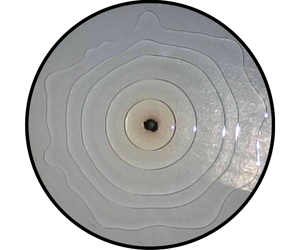
Snapshots of an experiment for a droplet volume of $V=80~\unicode[STIX]{x03BC}\text{l}$. The times are measured from the instant when the droplet is deposited on the substrate. (a) The flow is stable, and the contact line conserves the axial symmetry. (b) The instability starts to deform the contact line. Although the contour is not a perfect circle, the mean radius is still very representative of the position of the contact line. (c) As time elapses, the amplitude of the instability increases, and the contour becomes wavy. (d) Finally, the advancing front develops a finger-shaped pattern. (e) A side view allows us to see the ring-like shape adopted by the liquid.

Figure 3.

(a) Radius of the contact line $r_{f}$ as a function of time $t$ for all the experiments. The volume $V$ of the droplet was 10, 20, 30, 40, 50, 60, 70, 80, 90 and $100~\unicode[STIX]{x03BC}\text{l}$, the external radius of the substrates, $r_{2}$, took the value of 50 mm (▵) or 25 mm (○) and $\unicode[STIX]{x0394}T$ was between $73.2$ and $129.6\,^{\circ }\text{C}$. The black dots correspond to the isothermal case ($\unicode[STIX]{x0394}T=0$) and the black solid line corresponds to the best fit to $r_{f}\propto t^{1/8}$, as predicted in Lopez, Miller & Ruckenstein (Reference Lopez, Miller and Ruckenstein1976) and Cazabat & Stuart (Reference Cazabat and Stuart1986). The error in the determination of $r_{f}$ is ${\sim}0.3~\text{mm}$. (b) Double log plot of $\tilde{r}_{f}$ versus $\tilde{t}$ for the same experimental runs shown in (a), but for the isothermal case. The dashed black lines correspond to the curves $1.03\times t^{1/3}$ and $0.85\times t^{1/3}$. We used $\unicode[STIX]{x1D707}=1~\text{Pa}~\text{s}$, $\unicode[STIX]{x1D6FE}_{0}=21\times 10^{-3}~\text{N}~\text{m}^{-1}$ and $\unicode[STIX]{x1D70E}=5\times 10^{-5}~\text{N}~{\text{m}^{-1}~}^{\circ }\text{C}^{-1}$. The estimated values for $B$ range from 0.08 to 0.15. Typical values for the Biot, Péclet and capillary numbers are $0.04$, $0.05$ and $10^{-4}$, respectively.

The experimental procedure is as follows. The temperature distribution of the substrate is monitored with a FLIR^® SC660 thermal camera until a stationary state is reached. Then, a video camera starts to record, and a controlled volume of PDMS is deposited at the centre of the substrate by means of a micropipette. Centring is crucial for successful deposition, and it is ensured by observing the position of the micropipette tip from two perpendicular directions. When deposition at the centre fails, this is immediately revealed by an early asymmetric displacement of the fluid. The volume of the droplet ranges from $10$ to $100\pm 0.05~\unicode[STIX]{x03BC}\text{l}$. The experiment finishes when the liquid reaches the border of the substrate (Dominguez Torres et al. Reference Dominguez Torres, Garrido Gonzalez, Villa and Gomba2016; Mac Intyre Reference Mac Intyre2017). After each experiment, the PDMS is removed, and the glass is cleaned by immersion in a sulphochromic acid bath for four days to ensure removal of any oil residue on the glass surface. Finally, the glass is washed with distilled water, dried with hot air and immediately employed.

Figure 2 shows images of a typical experiment. All of our experiments show two consecutive well-differentiated regimes. In the first regime, the axial symmetry holds: the radius of the droplet increases (figure 2a), and a capillary ridge emerges close to the contact line. As the ridge moves, it leaves behind a very thin film of fluid, and what was initially a droplet is now better described as a ring (figure 2e). In the second regime, the advancing contact line becomes unstable, and smooth corrugations develop (figure 2b,c) such that the axial symmetry is broken. The amplitude of these corrugations increases with time, and the contact line finally adopts a finger-like pattern (figure 2d).

3 Stable regime

The reader may ask why such a ring-like profile develops. As previously stated, the thermal gradient of the substrate induces a surface tension gradient for the liquid, which in turn generates a radially outward flow. As we show later, the Marangoni effect scales as $h^{2}$, and since the thickness of the droplet is initially greater at the centre, the outward flow is stronger there than at the periphery of the droplet. Thus, liquid accumulates behind the contact line, and then a capillary ridge is formed, giving the surface of the fluid the shape of a ring. The emergence of a capillary ridge always occurs when the contact line of an unconfined film is driven by a force parallel to the substrate (Spaid & Homsy Reference Spaid and Homsy1996), independent of the nature of the force (gravitational, thermocapillary or centrifugal) and symmetry (planar or axial). In all cases, the ridge is the result of the accumulation of the liquid flowing towards the contact line.

Figure 3(a) shows the radius $r_{f}$ of the contact line as a function of time $t$ for $V=10$ to $100~\unicode[STIX]{x03BC}\text{l}$ (we also include the case with $\unicode[STIX]{x0394}T=0$ to visualise the difference in the spreading rate when the thermal gradient is not applied). The data show a regular behaviour that is physically interpreted as follows. We assume that the dynamics of the ring is governed by the balance between the Marangoni and viscous stresses. The Marangoni stress is estimated as $\unicode[STIX]{x1D70F}_{M}\sim \unicode[STIX]{x0394}\unicode[STIX]{x1D6FE}/w$, where $\unicode[STIX]{x0394}\unicode[STIX]{x1D6FE}$ is the variation in the surface tension across the width $w$ of the ridge. Since (i) PDMS shows a linear dependence of surface tension $\unicode[STIX]{x1D6FE}$ on temperature $\unicode[STIX]{x1D6FE}=\unicode[STIX]{x1D6FE}_{0}-\unicode[STIX]{x1D70E}(T-T_{0})$ (Darhuber et al. Reference Darhuber, Davis, Troian and Reisner2003), with $\unicode[STIX]{x1D70E}>0$ and the subscript zero denoting reference values, and (ii) $T$ varies logarithmically with $r$, it is possible to estimate $\unicode[STIX]{x0394}\unicode[STIX]{x1D6FE}$ to first order in $w$ to finally obtain

(3.1)$$\begin{eqnarray}\unicode[STIX]{x1D70F}_{M}\sim \frac{\unicode[STIX]{x1D70E}\unicode[STIX]{x0394}T}{r_{f}\ln (r_{2}/r_{1})}.\end{eqnarray}$$

The viscous stress is estimated as $\unicode[STIX]{x1D70F}_{v}\sim \unicode[STIX]{x1D707}(\text{d}r_{f}/\text{d}t)/h_{b}$, where $h_{b}$ is the height of the ridge and $\unicode[STIX]{x1D707}$ is the viscosity. Balancing the viscous and thermocapillary stresses, one obtains

(3.2)$$\begin{eqnarray}r_{f}\frac{\text{d}r_{f}}{\text{d}t}\sim \frac{h_{b}\unicode[STIX]{x1D70E}\unicode[STIX]{x0394}T}{\unicode[STIX]{x1D707}\ln (r_{2}/r_{1})}.\end{eqnarray}$$

Assuming that $w$ is constant and the liquid volume $V$ initially deposited at the centre of the substrate is contained in the ring (a negligible film is deposited as the ring advances), we obtain $V\sim h_{b}wr_{f}$. Then,

(3.3)$$\begin{eqnarray}r_{f}\sim \left(\frac{3\unicode[STIX]{x1D70E}\unicode[STIX]{x0394}TV}{\unicode[STIX]{x1D707}w\ln (r_{2}/r_{1})}t\right)^{1/3}=\left(\frac{2\unicode[STIX]{x1D6FE}_{0}BV}{\unicode[STIX]{x1D707}w}t\right)^{1/3}.\end{eqnarray}$$

Here, $B=3\unicode[STIX]{x1D70E}\unicode[STIX]{x0394}T/[2\unicode[STIX]{x1D6FE}_{0}\ln (r_{2}/r_{1})]$ is a dimensionless parameter that quantifies the strength of the thermocapillary effect, and it is experimentally obtained as $B=(3\unicode[STIX]{x1D70E}/2\unicode[STIX]{x1D6FE}_{0})\times a$.

Defining the dimensionless variables $\tilde{r}_{f}=r_{f}/r_{0}$, $\tilde{w}=w/r_{0}$ and $\tilde{t}=t/t_{0}$, where

(3.4a,b)$$\begin{eqnarray}r_{0}=\frac{V^{1/3}}{B^{1/6}},\quad t_{0}=\frac{3\unicode[STIX]{x1D707}V^{1/3}}{\unicode[STIX]{x1D6FE}_{0}B^{5/3}},\end{eqnarray}$$

equation (3.3) reduces to

(3.5)$$\begin{eqnarray}\tilde{r}_{f}\sim (6\tilde{t}/\tilde{w})^{1/3}.\end{eqnarray}$$

As shown numerically below, all the dimensionless thickness profiles collapse for long times, which implies that $\tilde{w}$ is the same for all experiments. Then, (3.5) predicts that the data shown in figure 3(a) must collapse onto a unique curve after dimensions are removed. To verify the relationship $\tilde{r}_{f}\propto \tilde{t}^{\,1/3}$ and the collapse of the data, we show in figure 3(b) a log–log plot of the data displayed in figure 3(a), but for the isothermal case, scaled according to (3.4). The curves fall between the two dashed lines given by $(0.94\pm 0.09)\times \tilde{t}^{\,1/3}$, showing a reasonable collapse of all of them onto a unique curve as predicted by (3.5), although with some dispersion. The parallel shift of the data from a unique curve is mainly due to the uncertainty in the temporal scale $t_{0}$, which strongly depends on $B$. Effectively, $t_{0}\propto B^{-5/3}$, and thus a $5\,\%$ error in the determination of $B$ results in an approximately $8\,\%$ uncertainty in the estimation of $t_{0}$.

We perform two-dimensional simulations to obtain the thickness profile $\tilde{h}=\tilde{h}(\tilde{r},\tilde{t})$ by applying the lubrication approximation to the Navier–Stokes equations, i.e. disregarding inertia and assuming that the liquid surface has a gentle slope (Gotkis et al. Reference Gotkis, Ivanov, Murisic and Kondic2006). Since PDMS completely wets the substrate, disjoining–conjoining pressure terms are not present in the modelling (Cazabat et al. Reference Cazabat, Heslot, Troian and Carles1990; Diez & Kondic Reference Diez and Kondic2001; Sur, Witelski & Behringer Reference Sur, Witelski and Behringer2004). The framework of our model is as follows. (i) Conduction is the main heat transfer mechanism within the droplet (which implies a small Péclet number $Pe=h_{c}U_{c}/\unicode[STIX]{x1D6FC}$), and the conductivity of the liquid, $k_{l}$, is high (i.e. we have a small Biot number $Bi=q_{s}h_{c}/k_{l}$). Here, $h_{c}$ and $U_{c}$ are the characteristic thickness and velocity, respectively, $\unicode[STIX]{x1D6FC}$ is the thermal diffusivity and $q_{s}$ is the liquid–air heat transfer coefficient. Then, the temperature of the liquid surface is identical to that of the substrate, a usual condition found in experiments of thin PDMS films and droplets driven by thermocapillarity (Cazabat et al. Reference Cazabat, Heslot, Troian and Carles1990; Brzoska et al. Reference Brzoska, Brochard-Wyart and Rondelez1993; Sur et al. Reference Sur, Witelski and Behringer2004; Chen et al. Reference Chen, Troian, Darhuber and Wagner2005). (ii) Since the surface tension depends linearly on temperature, the Marangoni stress at the liquid–air interface is $\unicode[STIX]{x1D70F}=2\unicode[STIX]{x1D6FE}_{0}B\unicode[STIX]{x1D6FF}/(3r)$, with $\unicode[STIX]{x1D6FF}=1$ for $r>r_{1}$ and $\unicode[STIX]{x1D6FF}=0$ for $r<r_{1}$. (iii) At the liquid–solid interface, we impose the no-slip condition. (iv) We assume the existence of an infinitely extended precursor film with uniform thickness (Diez & Kondic Reference Diez and Kondic2001; Mac Intyre et al. Reference Mac Intyre, Gomba, Perazzo, Correa and Sellier2018). In this way, we avoid divergence of the stress at the contact line. More importantly, we include in the modelling an experimentally well-proven fact: when a completely wetting liquid spreads slowly enough on a clean smooth surface, a very thin precursor film propagates ahead of the macroscopic contact line faster than it and prewets the solid substrate (see, for example, Popescu et al. (Reference Popescu, Oshanin, Dietrich and Cazabat2012) and references therein). The extension of the precursor film is finite, but as its dynamics is decoupled from the spreading of the bulk, it is usually considered to cover the whole domain (Spaid & Homsy Reference Spaid and Homsy1996). In particular, the existence of a precursor film in the case of PDMS on glass is confirmed in Hoang & Kavehpour (Reference Hoang and Kavehpour2011).

Defining the dimensionless variables $\tilde{r}=r/r_{0}$ and $\tilde{h}=h/h_{0}$, with $h_{0}=V^{1/3}B^{1/3}$, the evolution of the dimensionless thickness $\tilde{h}=\tilde{h}(\tilde{r},\tilde{t})$ of the liquid is governed by (see Gomba & Homsy (Reference Gomba and Homsy2010) for details of the numerical implementation)

(3.6)$$\begin{eqnarray}\displaystyle & \displaystyle 0=\frac{\unicode[STIX]{x2202}\tilde{h}}{\unicode[STIX]{x2202}\tilde{t}}+\frac{1}{\tilde{r}}\frac{\unicode[STIX]{x2202}}{\unicode[STIX]{x2202}\tilde{r}}\left(-\tilde{r}\tilde{h}^{3}\frac{\unicode[STIX]{x2202}p}{\unicode[STIX]{x2202}\tilde{r}}+\unicode[STIX]{x1D6FF}\tilde{h}^{2}\right), & \displaystyle\end{eqnarray}$$

(3.7)$$\begin{eqnarray}\displaystyle & \displaystyle p=-\frac{1}{\tilde{r}}\frac{\unicode[STIX]{x2202}}{\unicode[STIX]{x2202}\tilde{r}}\left(\tilde{r}\frac{\unicode[STIX]{x2202}\tilde{h}}{\unicode[STIX]{x2202}\tilde{r}}\right). & \displaystyle\end{eqnarray}$$

Note that (3.6) and (3.7) are parameter free, which justifies the definition of $r_{0}$, $h_{0}$ and $t_{0}$. Additionally, with these scales, the volume is equal to unity. This two-dimensional model, derived from a three-dimensional continuity equation, ensures mass conservation in the axisymmetric geometry.

Figure 4.

(a) Numerical solution of (3.6) and (3.7). The initial profiles are centred parabolas with height 1 (blue) or 0.5 (red) over a precursor film whose thickness is $10^{-4}$. Inset: a zoom-in of the thickness profile for $\tilde{t}=100$ (red solid line) and the outer solution $\tilde{h}_{outer}$, equation (3.9) (black dashed line). Here $\tilde{h}_{m}$ is the thickness at the point at which $\tilde{h}_{outer}$ matches the ridge region thickness. (b) Contact line position, $\tilde{r}_{f}$, and maximum thickness of the ridge, $\tilde{h}_{b}$, for simulations with initial thickness profiles with a maximum height equal to 1 (blue), 0.75 (green), 0.5 (red) and 0.35 (cyan). The best fits to $\tilde{r}_{f}\propto t^{n}$ and $\tilde{h}_{b}\propto t^{m}$ for $10\leqslant \tilde{t}\leqslant 100$ give exponents $n=0.334\pm 0.002$ and $m=-0.374\pm 0.018$. The dashed lines have slopes $\pm 1/3$.

We speculate that, at a sufficiently long time, the flow loses memory of its initial profile. Therefore, since (3.6) and (3.7) have no parameters, all solutions should asymptotically show the same behaviour. To test this hypothesis, we numerically solved these equations assuming an initial parabolic profile with different aspect ratios. Figure 4(a) shows numerical solutions for two different initial profiles with maximum initial heights equal to $0.5$ and $1$. Remarkably, for $\tilde{t}\geqslant 25$, the solutions collapse onto a single profile. Additionally, after an initial stage, a capillary ridge that corresponds to a cross-section of the ring emerges and advances, leaving a thin liquid layer behind. Figure 4(b) shows the (numerical) position of the contact line $\tilde{r}_{f}$ as a function of time for four different runs. For large $\tilde{t}$, $\tilde{r}_{f}\propto \tilde{t}^{\;1/3}$, in agreement with the experiments, and the maximum thickness of the ridge $\tilde{h}_{b}$ decreases as $\tilde{t}^{-0.374}$, very close to the law $\tilde{t}^{-1/3}$ expected from assuming that the volume within the ring and $\tilde{w}$ remain constant. The good collapse of the numerical runs onto a unique curve $\tilde{r}_{f}$ versus $\tilde{t}$ reinforces the hypothesis that the weak dispersion observed in figure 3(b) comes from the measurement error in $B$.

Figure 5.

(a) Radius $\tilde{r}_{f,c}$ at which the contact line becomes unstable. Note that $\tilde{r}_{f,c}$ is approximately constant for all the explored volumes. (b) Standard deviation (SD) of $\tilde{r}_{f}$ against the mean radius of the contour, $\langle \tilde{r}_{f}\rangle$. The standard deviation remains almost unchanged until $\langle \tilde{r}_{f}\rangle \approx 3$, at which point it starts to increase. Inset: a zoom-in for the case of $V=50~\unicode[STIX]{x03BC}\text{l}$. The value of $\tilde{r}_{f,c}$ is estimated as the intersection of the two solid lines, as explained in the text.

Following Mac Intyre et al. (Reference Mac Intyre, Gomba, Perazzo, Correa and Sellier2018), we find the outer solution for the thickness profile by disregarding the effect of the curvature in the region behind the capillary ridge. Then, we search for the asymptotic solution to

(3.8)$$\begin{eqnarray}\frac{\unicode[STIX]{x2202}\tilde{h}}{\unicode[STIX]{x2202}\tilde{t}}+\frac{1}{\tilde{r}}\frac{\unicode[STIX]{x2202}\tilde{h}^{2}}{\unicode[STIX]{x2202}\tilde{r}}=0,\end{eqnarray}$$

which represents the competition between the viscous and Marangoni stresses outside the ridge region. We obtain the outer solution as

(3.9)$$\begin{eqnarray}\tilde{h}_{outer}=\tilde{r}^{2}/(4\tilde{t}).\end{eqnarray}$$

The inset of figure 4(a) shows that outside the ridge region, there is excellent agreement between the outer solution and the numerical solution of (3.6) and (3.7).

4 Unstable regime

After advancing symmetrically for some time, we observe the emergence of undulations at the contact line, which are usually attributed to weak perturbations at the capillary ridge (Troian, Joanny & Safran Reference Troian, Joanny and Safran1989; Brzoska et al. Reference Brzoska, Brochard-Wyart and Rondelez1993; Spaid & Homsy Reference Spaid and Homsy1996). Figure 5(a) shows the critical radius of the front, $\tilde{r}_{f,c}$, at which onset of the instability is detected. To measure $\tilde{r}_{f,c}$, we digitised the contact line of the droplet at different times, with each contour consisting of 1000 points. For each contour, we measured the mean radius and its standard deviation. The critical radius of each experiment is defined as the radius at which the standard deviation starts to increase, a value that is determined by the intersection of two straight lines, the first one fitting the initial (constant) standard deviation and the second one fitting the first points above that line, as shown for the case with $V=50~\unicode[STIX]{x03BC}\text{l}$ in the inset of figure 5(b). We observe that the standard deviation remains approximately constant until $\langle \tilde{r}_{f}\rangle =\tilde{r}_{f,c}\approx 3$, at which point it starts to increase independent of $V$ or $\unicode[STIX]{x0394}T$ (this fact gives additional support to the adopted scaling). To discard boundary effects on the emergence of the instability, we checked that it occurred no less than 2.15 cm from $r_{2}$, except in one case with $V=50~\unicode[STIX]{x03BC}\text{l}$, $r_{2}=2.5~\text{cm}$ and $r_{f,c}=1.08~\text{cm}$. In most cases, $r_{2}/r_{f,c}\geqslant 2.2$.

Figure 6.

Number of fingers versus $\langle \tilde{r}_{f}\rangle$. The fit of the points to $N_{f}=c\times \langle \tilde{r}_{f}\rangle$, which gives $c=1.61$, is represented by the dashed line.

The instability of the contact line is usually characterised by counting the number of undulations or ‘fingers’ $N_{f}$ observed at the end of the experiment (Melo et al. Reference Melo, Joanny and Fauve1989; Fraysse & Homsy Reference Fraysse and Homsy1994; Sur et al. Reference Sur, Witelski and Behringer2004). However, since $N_{f}$ increases with time, we instead evaluated $N_{f}$ against the mean dimensionless radius. The result is shown in figure 6 (for each experiment, we analysed contours at two arbitrary times, at approximately the halfway point and close to the end of the experiment). The value of $N_{f}$ increases roughly linearly with $\langle \tilde{r}_{f}\rangle$.

As previously mentioned, the formation of a capillary ridge and its subsequent destabilisation are omnipresent in unconfined flows involving advancing three-phase contact lines. To explain the linear dependence of $N_{f}$ on $\langle \tilde{r}_{f}\rangle$, we use some results of the general procedure formulated by Troian et al. (Reference Troian, Joanny and Safran1989), in which the authors address the linear stability of a capillary ridge. Their scaling and method have been successfully applied to problems with various driving forces and symmetries (e.g. flows down an inclined plane or axisymmetric centrifugal coatings). We devote the following paragraph to presenting the main ideas of their analysis that we later apply to our case.

Troian and co-authors consider two regions in the flow: (a) an ‘outer’ region, where the thickness profile is determined by the competition between the driving force and the viscous stress, and (b) an ‘inner’ region, where the capillary and driving force terms balance, forming a ridge (they identify this region as being responsible for the instability). Within the lubrication approximation, the balance in the inner region reads

(4.1)$$\begin{eqnarray}\boldsymbol{v}\sim \frac{\unicode[STIX]{x1D6FE}}{3\unicode[STIX]{x1D707}}h^{2}\unicode[STIX]{x1D735}\unicode[STIX]{x1D6FB}^{2}h,\end{eqnarray}$$

where $\boldsymbol{v}$ is the velocity associated with the driving force. Denoting $h_{m}$ as the characteristic thickness at the point at which the inner and outer regions meet and $U$ as the characteristic advancing velocity of the outer solution, (4.1) gives the length scale $\ell$ for the inner region: $U\approx \unicode[STIX]{x1D6FE}/(3\unicode[STIX]{x1D707})\times h_{m}^{3}/\ell ^{3}$; then, $\ell =h_{m}\times (3Ca)^{-1/3}$, with $Ca=\unicode[STIX]{x1D707}U/\unicode[STIX]{x1D6FE}$ being the capillary number. Note that this definition for $\ell$ is independent of the nature of the driving force and is valid for both polar and Cartesian coordinates (i.e. axisymmetric or straight liquid distributions). What is characteristic of each force is the behaviour of $h_{m}$ and $U$ (Troian et al. Reference Troian, Joanny and Safran1989; Spaid & Homsy Reference Spaid and Homsy1996). Finally, the scaled inner region is employed as the base state for a standard linear stability analysis. Examples of the application of the method of Troian et al. (Reference Troian, Joanny and Safran1989) to analyse the stability of the capillary ridge for various driving forces and symmetries include Fraysse & Homsy (Reference Fraysse and Homsy1994), Brzoska, Brochard-Wyart & Rondel (Reference Brzoska, Brochard-Wyart and Rondel1992) and Cazabat et al. (Reference Cazabat, Heslot, Troian and Carles1990). Interestingly for our problem, in all these works, the authors find that (a) the dispersion relationship has a single dominant wavelength and (b) since $\ell$ is the typical scale for the inner (ridge) region, the most unstable wavelength also scales with $\ell$, i.e. $\unicode[STIX]{x1D706}_{max}\propto \ell$.

Refocusing on our problem, to capture the main dependence of $N_{f}$ on $\langle \tilde{r}_{f}\rangle$, we use the results from Troian et al. (Reference Troian, Joanny and Safran1989). The number of fingers is given by

(4.2)$$\begin{eqnarray}N_{f}=L/\unicode[STIX]{x1D706}_{max}\propto L/\ell =L/[h_{m}\times (3Ca)^{-1/3}]\propto LU^{1/3}/h_{m},\end{eqnarray}$$

where $L=2\unicode[STIX]{x03C0}r_{0}\langle \tilde{r}_{f}\rangle$ is the dimensional length of the contact line. Expressed in dimensionless quantities, (4.2) becomes

(4.3)$$\begin{eqnarray}N_{f}\propto \langle \tilde{r}_{f}\rangle \tilde{U} ^{1/3}/\tilde{h}_{m},\end{eqnarray}$$

where $\tilde{U} =Ut_{0}/r_{0}$ is the dimensionless velocity of the outer solution. We obtain $\tilde{h}_{m}(\tilde{t})$ from the simulation as the thickness at the point at which $\tilde{h}_{outer}$ starts to differ by more than $0.5\,\%$ of the complete profile, which is marked with a black point in the inset of figure 4(a). We found that $\tilde{h}_{m}\propto \tilde{t}^{-0.194}$ and that it advances with a velocity $\tilde{U} \propto \tilde{t}^{-0.546}$. Substituting these power laws into (4.3) leads to $N_{f}\propto \langle \tilde{r}_{f}\rangle \tilde{t}^{-0.012}$, and since this is a weak dependence on time, it is reasonable to consider $N_{f}\propto \langle \tilde{r}_{f}\rangle$.

In figure 6, the fit to the data gives $N_{f}=1.61\times \langle \tilde{r}_{f}\rangle$. This result is surprisingly close to that reported by Pairam & Fernández-Nieves (Reference Pairam and Fernández-Nieves2009) for the instability of static isothermal rings. Those authors observed that the mode with the largest growth rate promotes breakup of the rings into $N_{d}$ droplets, and they found $N_{d}=0.57\times 2r/w$. Note that from figure 4(a), $\tilde{w}\approx 0.8$, so $N_{d}=1.425\times \tilde{r}$, which is comparable to our results, despite the differences between the two scenarios.

Considering the different $V$ and $B$ of our experiments, the dimensional scale $\tilde{\ell }h_{0}=0.053h_{0}$ is in the range of $50{-}130~\unicode[STIX]{x03BC}\text{m}$, comparable to the values reported by Brzoska et al. (Reference Brzoska, Brochard-Wyart and Rondel1992) for experiments on straight strips of fluids under the effect of uniform thermal gradients. This is reasonable because the width of the ring is much less than its radius, so the ring can be considered locally straight and the thermal gradient locally uniform.

5 Discussions and conclusions

We report experiments on the axial spreading of a fluid driven by radial thermocapillary stress. The advance of the front follows a power-law relationship that is explained in terms of the balance between the viscous and Marangoni stresses. Interestingly, while for liquid strips under constant temperature gradients the instabilities appear almost immediately (Brzoska et al. Reference Brzoska, Brochard-Wyart and Rondel1992), here, for a stress that decreases as $1/r$, we observe that the instability takes some time to begin. The onset of the instability occurs at the dimensional radius $r_{f,c}\approx 3\times V^{1/3}/B^{1/6}$, i.e. the volume of the liquid is the main parameter determining the end of the stable spreading.

The simulations capture the dynamics of the spreading and reproduce the $t^{1/3}$ dependence of the front. They also show that the height of the ridge decreases as $t^{-0.374}$, so the product $h_{b}\times r_{f}$ is almost independent of $t$, which supports the assumption about the approximately constant width of the ring. The simulations show that after a short initial stage, the thickness profiles collapse onto a unique asymptotic profile, whose outer region is well represented by (3.9).

Figure 7.

Evolution of the Fourier spectra for two different volumes: $V=40~\unicode[STIX]{x03BC}\text{l}$ (a) and $V=80~\unicode[STIX]{x03BC}\text{l}$ (b). The azimuthal wavenumber with the maximum amplitude shifts to larger values as the experiment evolves.

The change in the dominant azimuthal wavenumber $L/\unicode[STIX]{x1D706}_{max}$ (that we identified, as a first approach, as the number of fingers) with the perimeter in the experiments can be observed by taking a Fourier transform of the contact line at different times (as carried out by Fraysse & Homsy (Reference Fraysse and Homsy1994) and Gomba et al. (Reference Gomba, Diez, Gratton, González and Kondic2007) for spin- and gravity-driven spreading, respectively). In figure 7, we show the evolution of the spectra for two different volumes, where we computed the fast Fourier transform as defined in equation (3) of Fraysse & Homsy (Reference Fraysse and Homsy1994). Effectively, the azimuthal wavenumber with the largest amplitude increases with $t$ or, equivalently, with $\langle r_{f}\rangle$. Interestingly, this shift of the dominant wavenumber towards larger values is not observed in centrifugal spreading (Fraysse & Homsy Reference Fraysse and Homsy1994): once one mode exhibits the maximum amplitude, its growth is favoured by the centrifugal force that increases with $r$, meaning that the fluid at the largest radius position ‘feels’ the strongest centrifugal stress. In contrast, in our experiments, the driving force is proportional to $1/r$, and thus a portion of fluid in the tip of a finger is under a smaller driving force than that at the valley between fingers. This explains why an increase of the maximum-amplitude wavenumber can occur in our experiments, a phenomenon that is not observed in experiments with films driven by constant forces (Huppert Reference Huppert1982; Gomba et al. Reference Gomba, Diez, González and Gratton2005, Reference Gomba, Diez, Gratton, González and Kondic2007).

Clearly, if no thermal gradient is applied, then a ring does not form. Therefore, one may wonder if $B$ must be larger than a critical value for a ring to develop. As explained in § 3, all the solutions of (3.6) and (3.7) converge to the same ring-like profile. Therefore, as these equations are parameter free, this is true for any value of $B$, and such a critical value does not exist. However, this conclusion is contingent on the validity of the assumptions of our model. For example, if the droplet is very small and the thermal gradient is very weak, then the liquid could coat the substrate with a monomolecular layer, a situation that cannot be described by (3.6) and (3.7). Thus, from the theoretical point of view, we conclude that a ring will always arise if the assumptions of our model are fulfilled. However, even in this case, inspection of the dependence of the scales $r_{0}$, $t_{0}$ and $h_{0}$ on $B$ reveals that if $B$ is too small, then the ring would emerge extremely late, with a very large radius and a tiny thickness, so the ring could be imperceptible.

All the present work involves complete wettability, i.e. null steady contact angle $\unicode[STIX]{x1D703}$. Future work may involve flows with $\unicode[STIX]{x1D703}>0$. To consider partial wetting fluids in our numerical model, a conjoining–disjoining pressure must be added to (3.7) (Mac Intyre et al. Reference Mac Intyre, Gomba, Perazzo, Correa and Sellier2018). We have done this for various contact angles $\unicode[STIX]{x1D703}$, and our preliminary simulations for $5^{\circ }<\unicode[STIX]{x1D703}<13^{\circ }$ show that $\tilde{r}_{f}\propto \tilde{t}^{2/5}$ and that both $\tilde{h}_{b}$ and $\tilde{w}$ decrease $\propto \tilde{t}^{-1/5}$ ($\tilde{w}$ does not remain constant as for $\unicode[STIX]{x1D703}=0$). Another point to address in the future is the exploration of the potential of using our method to coat surfaces as an alternative to spin coating, especially in cases where rotating the substrate is not a feasible option.