
1. Introduction
Dispersed multiphase flows cover a vast field that concerns many industrial processes (bubble columns, fluidized beds, heat exchangers $\ldots$) as well as natural processes (breaking waves, rains, avalanches
 $\ldots$). This presence in very varied fields has favoured a significant development of experimental and numerical methods to investigate these types of flows (Mudde Reference Mudde2005; Balachandar & Eaton Reference Balachandar and Eaton2010; Elghobashi Reference Elghobashi2018; Risso Reference Risso2018).
In this work, we focus on flows involving large bubbles. By large, we mean that the Reynolds number based on the bubble size and terminal velocity is several hundred such that each bubble generates a strong wake. In such a situation, the liquid fluctuations induced by the bubbles are essentially driven by the interactions between the wakes (Riboux, Risso & Legendre Reference Riboux, Risso and Legendre2010; Riboux, Legendre & Risso Reference Riboux, Legendre and Risso2013; Amoura et al. Reference Amoura, Besnaci, Risso and Roig2017). These interactions cause a very pronounced wake screening by the neighbouring bubbles (Hunt & Eames Reference Hunt and Eames2002), which leads to an exponential decay of the wakes with the distance to the bubble (Risso et al. Reference Risso, Roig, Amoura, Riboux and Billet2008). Moreover, the interactions lead to a collective instability of the liquid flow among the bubbles, which gives birth to turbulent fluctuations. For a homogeneous swarm of rising bubbles, the localized flow disturbances generated around the bubbles and the bubble-induced turbulence constitute the two sources of liquid fluctuations. These fluctuations show very specific properties which have been revealed by experimental investigations (Lance & Bataille Reference Lance and Bataille1991; Zenit, Koch & Sangani Reference Zenit, Koch and Sangani2001; Garnier, Lance & Marié Reference Garnier, Lance and Marié2002; Risso & Ellingsen Reference Risso and Ellingsen2002; Rensen, Luther & Lohse Reference Rensen, Luther and Lohse2005; Martínez Mercado, Palacios-Morales & Zenit Reference Martínez Mercado, Palacios-Morales and Zenit2007; Riboux et al. Reference Riboux, Risso and Legendre2010; Mendez-Diaz et al. Reference Mendez-Diaz, Serrano-García, Zenit and Hernández-Cordero2013; Prakash et al. Reference Prakash, Martínez Mercado, van Wijngaarden, Mancilla, Tagawa, Lohse and Sun2016; Alméras et al. Reference Alméras, Mathai, Lohse and Sun2017). The kinetic energy is roughly proportional to the product of the gas volume fraction  $\alpha$ and the square of the average bubble rise velocity
 $v_0$. The liquid velocity fluctuations are highly anisotropic, with vertical fluctuations more intense than horizontal ones. Their probability density functions (p.d.f.s) are non-Gaussian, with exponential tails and a strong dissymmetry between upward and downward directions. Their power spectrum evolves as
 $k^{-3}$ in a subrange of wavenumbers
 $k$ spreading around the bubble diameters, where a maximum of energy is injected. Moreover, when normalized by the variance of the fluctuations, the spectrum is independent of
 $\alpha$, which implies that the same is true for the integral scale of the flow. The origin of such a scaling law as well as its precise boundaries in the spectral domain remain poorly understood.
The statistical properties of the motion of the dispersed phase have also been characterized by the experiments cited above. In a homogeneous swarm of bubbles, the average bubble rising speed decreases when the volume fraction increases. Regarding the bubble velocity fluctuations, it is important to recall that provided the bubble deformation and Reynolds number are beyond a given threshold (Zenit & Magnaudet Reference Zenit and Magnaudet2008), the wake becomes unstable and the bubble performs path oscillations. As soon as wake instabilities are present, which is the case for air bubbles with sizes of a few millimetres in water, this mechanism is the main cause of bubble velocity fluctuations and that remains true even at a volume fraction as large as 30 % (Colombet et al. Reference Colombet, Legendre, Risso, Cockx and Guiraud2015). These wake-induced fluctuations are probably the reason why stable homogeneous bubbly flows can easily be generated in laboratory bubble columns (van Wijngaarden Reference van Wijngaarden2005). Indeed, the horizontal clusters that are expected to form due to potential interactions between large-Reynolds-number bubbles are prevented by the strong path oscillations resulting from the wake instabilities (Yurkovetsky & Brady Reference Yurkovetsky and Brady1996; Sangani & Didwania Reference Sangani and Didwania2006). However, the stability of homogeneous bubble columns is limited to reasonably small geometry with well-controlled uniform bubble injection. In most industrial applications, the gas volume fraction is not homogeneous all over the flow and buoyancy-driven large-scale motions develop (Mudde Reference Mudde2005).
Because of the limitations of experimental measurement techniques due to the presence of many interfaces, advances in the understanding of the mechanisms of the turbulence generated by the bubbles are expected to come from numerical simulations. Nevertheless, the numerical simulation of bubbly flows at large Reynolds numbers remains challenging. The difficulty lies in the diversity of the length scales present in this type of flow, especially when we are interested in describing both the fluctuations at the bubble scale and the motions induced by the gradient of the gas volume fraction at the scale of the container. Direct numerical simulation (DNS) approaches, in which all scales of the flow as well as the interfacial dynamics are properly solved, are too greedy in computing resources and are limited to a small number of bubbles and a low Reynolds number. Another approach consists of considering the continuous liquid phase and the dispersed gas phase separately, which leads to the Euler–Lagrange framework. In this case, the resolution of the flow details at scales smaller than that of the diameter is replaced by a modelling step. Most of the previous works based on the Euler–Lagrange approach consider dispersed objects (bubbles, particles, droplets) with a small Reynolds number (Balachandar & Eaton Reference Balachandar and Eaton2010; Subramaniam Reference Subramaniam2013).
As discussed above, the wake interactions are essential and the work of Riboux et al. (Reference Riboux, Legendre and Risso2013) showed that considering only them can be relevant to perform large-scale Euler–Lagrange simulations of bubbly flows. They simulated the flow through a fixed random array of bubbles, with a bubble Reynolds number of a few hundred and a mesh spacing of the order of the bubble size. Therefore, in their approach, the scales close to or smaller than the bubble diameter are not resolved, but the downstream part of the wake is correctly described. Their results showed that the interaction between the bubbles wakes is well reproduced and that statistics of the large scales of the simulated flow are in relatively good agreement with the experiments of Riboux et al. (Reference Riboux, Risso and Legendre2010).
In this paper, we pursue this approach upon which we will improve by allowing the bubbles to move, so that their relative motion can be described. This is indeed an essential step if we want to be able to calculate the evolution of the void fraction as well as the formation of large-scale heterogeneity. As usual in Euler–Lagrange approaches, the tracking of the trajectory of each bubble requires a calculation of the hydrodynamic forces exerted on it. The models for these forces rely on the notion of undisturbed fluid velocity at the bubble position. This concept is in general not rigorously defined and can be understood as the velocity that the fluid would have at this location in the absence of this bubble. It appears thus necessary to estimate the flow disturbance caused by each particle composing the dispersed phase, in order to properly compute the hydrodynamic force. In many previous works using the Euler–Lagrange framework, this correction was neglected and the actual fluid velocity was used instead of the undisturbed fluid velocity, which leads to a spurious self-induced force. Indeed, in the case of small-Reynolds-number objects, it was shown (Saffman Reference Saffman1973; Boivin, Simonin & Squires Reference Boivin, Simonin and Squires1998) that this effect scales as the ratio of the particle diameter to the mesh-grid spacing and can thus be neglected for sufficiently small objects or coarse meshes. Furthermore, models have been recently proposed to correct the fluid phase velocity in the case of small-Reynolds-number particles (Capecelatro & Desjardins Reference Capecelatro and Desjardins2013; Onishi, Takahashi & Vassilicos Reference Onishi, Takahashi and Vassilicos2013; Gualtieri et al. Reference Gualtieri, Picano, Sardina and Casciola2015; Horwitz & Mani Reference Horwitz and Mani2016; Balachandar, Liu & Lakhote Reference Balachandar, Liu and Lakhote2019) and will be reviewed later in this paper. In our case, each bubble is modelled as a volume source of momentum distributed over a few mesh-grid elements to reproduce the bubble wake. It is therefore mandatory to correct the self-induced force. To this end, we propose in this paper an integral model to compute the flow disturbance due to a large bubble Reynolds number.
We stress that our emphasis is on the reproduction of the far field of each bubble because it is the one that interacts with the wakes of the other bubbles. Our method is designed so that the correct amount of momentum is transferred from each bubble to the fluid and that the interactions between the bubble wakes are described at the relevant scale. The principal objective of this work is to tackle the problem of spurious self-induced force to open the way of Euler–Lagrange simulations of dispersed two-phase flows, which are a natural framework to develop large-scale simulations of bubbly flows. Indeed, as soon as the scales smaller than the bubble are not resolved, the force acting on the bubbles cannot be computed by integration of the stress over its surface and a model of hydrodynamic force is required to move the dispersed phase. Note that, in the present paper, the method will be validated in the case of a homogeneous bubble swarm by comparison with the experimental results of Riboux et al. (Reference Riboux, Risso and Legendre2010). Thus, the model of hydrodynamic force will include drag, added mass, buoyancy and Tchen forces, but will not account for lift force. Also, fluctuations of bubble shape, breakup and coalescence will not be considered in this work.
Before getting to the heart of the matter, let us make a brief digression by making an analogy between one-way and two-way coupling in dispersed two-phase flows and a similar problem encountered in electromagnetism, which has stimulated our reflection. In electromagnetism, one usually considers two types of problems when fields and charged particles interact (Landau & Lifshitz Reference Landau and Lifshitz1975; Jackson Reference Jackson1999): either the fields are imposed and the evolution of the particle is studied, or the particle motion is prescribed and the field radiated by this particle is investigated. These two uncoupled approaches often give very acceptable results. However, when one studies the effect of the radiated field on the dynamics of the particle, one very often meets difficulties related to the self-induction force, which leads to the introduction of the Abraham–Lorentz or ‘radiation reaction’ force (Jackson Reference Jackson1999). This self-induced force is a convenient intermediary for estimating the influence of the radiation upon the particle motion, but it must be used with caution and always in a perturbative approach, as it can lead to non-physical solutions. In all cases, a more complete resolution of this problem must be based on quantum mechanics. In the Euler–Lagrange approaches for two-phase dispersed flows, one can either impose the flow field and study the evolution of the motion of a particle (one-way coupling) or prescribe the particles trajectories and study the induced velocity field (reverse one-way coupling as in Riboux et al. Reference Riboux, Legendre and Risso2013). In these cases, there are no ambiguities on the calculation of the hydrodynamic force. However, in the two-way coupling case, the problem of the interaction of the particle with the flow disturbance it generates itself arises too. When the velocity disturbance is weak compared to the flow that would exist in the absence of this particle, the self-induced force can simply be neglected. When it is possible to determine the disturbance caused by each single particle, a perturbative approach can allow us to obtain an accurate calculation of the force, as is the case in the present paper. But in general, the coupling between the two phases is well treated in changing the level of description, which requires abandoning the Euler–Lagrange framework and adopting instead a finer description of the problem allowing modelling of the dynamics inside the particles, as is the case with particle-resolved DNS. Note that, in any case, the model introduced to keep the Lagrangian formalism for the description of the particles needs to be invariant for a change of the reference frame. In electromagnetism, insuring Lorentz invariance requires the introduction of delayed potential (Landau & Lifshitz Reference Landau and Lifshitz1975). In multiphase flow, we shall also need to introduce a delayed interaction to preserve Galilean invariance.
Classic expressions of hydrodynamic forces acting on bodies rely on the definition of the fluid velocity that is undisturbed by the presence of this body. This concept of undisturbed velocity is thus a fundamental issue for dispersed two-phase flows. At large Reynolds number, the nonlinearity of the Navier–Stokes equations constitutes a bottle neck for physical modelling where a local drift velocity is often introduced and attempted to be measured by experiments and DNS (Merle, Legendre & Magnaudet Reference Merle, Legendre and Magnaudet2005; Naso & Prosperetti Reference Naso and Prosperetti2010; Loisy & Naso Reference Loisy and Naso2017; Huck et al. Reference Huck, Bateson, Volk, Cartellier, Bourgoin and Aliseda2018), as well as for performing large-scale simulations in which objects have to be transported without knowing the details of the flow around them.
The paper is organized as follows. Section 2 recalls the Euler–Lagrange formalism, discusses the relevance of this approach for the bubble-induced agitation, examines the modelling issue caused by the self-induced forces and presents a model to estimate the undisturbed fluid velocity in the vicinity of a bubble. Section 3 presents the numerical implementation of the model and its validation in the case of one or two bubbles rising in a quiescent liquid. Section 4 presents the results of the Euler–Lagrange simulation of a swarm of rising bubbles and its validation based on comparisons with experimental results.
2. Modelling approach
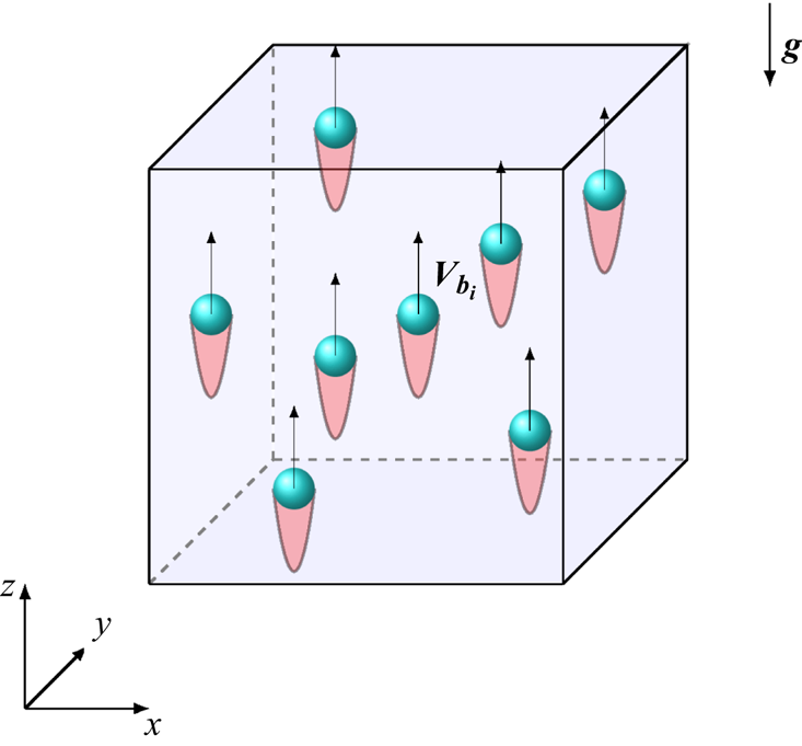
In this section, we present the method adopted in this paper to simulate a bubble swarm within the Euler–Lagrange framework (see the scheme in figure 1). In this framework, the bubbles are considered as volume sources of momentum. We propose a model to correct the spurious self-induced effect and accurately compute the hydrodynamic force applied on each bubble. This model is designed for large-Reynolds-number bubbles.
Schematic view of a rising swarm of bubbles. At large bubble Reynolds number, a strong wake develops behind each bubble.

As discussed in § 1, the agitation caused by the rise of a swarm of bubbles is dominated by wake interactions. We consider that it is not necessary to accurately describe the hydrodynamics in the direct vicinity of the bubbles to satisfactorily predict the bubble-induced agitation in the rest of the flow as long as the far-wake downstream of each bubble is correctly reproduced, because it is this part which actually intervenes in the interactions between wakes. In this study, the discussion is mainly focused on bubbly flows, but the present method is also applicable to other dispersed objects, such as droplets or solid particles.
2.1. Continuous phase
Assuming that the continuous phase is an incompressible Newtonian fluid, its dynamics is described by the Navier–Stokes equations,
 $$\begin{gather} \boldsymbol{\nabla}\boldsymbol{\cdot}{\boldsymbol{u}} = 0, \end{gather}$$
 $$\begin{gather}\frac{\partial\boldsymbol{u}}{\partial t} + \boldsymbol{\nabla}\boldsymbol{\cdot} (\boldsymbol{u} \boldsymbol{u}) ={-}\frac{1}{\rho}\boldsymbol{\nabla} P + \boldsymbol{\nabla}\boldsymbol{\cdot}\left( \nu \left[ \boldsymbol{\nabla}\boldsymbol u + \left(\boldsymbol{\nabla}\boldsymbol u \right)^{\textrm{T}} \right]\right) + \boldsymbol{g}, \end{gather}$$
where  $\boldsymbol {u}$ and
 $p$ are the velocity and pressure fields of the continuous phase,
 $\rho$ and
 $\nu$ its density and kinematic viscosity, and
 $\boldsymbol {g}$ the gravity acceleration. Nevertheless, these equations are to be complemented with very complex boundary conditions that evolve as the bubbles move in response to the fluid stress applied on their interface. When the number of dispersed objects remains limited, one can rely on fully resolved numerical simulations that accurately track the interfaces (Tenneti & Subramaniam Reference Tenneti and Subramaniam2014; Maxey Reference Maxey2017). To date, the number of objects that can be simulated is around 1000 (Lucci, Ferrante & Elghobashi Reference Lucci, Ferrante and Elghobashi2010; Uhlmann & Chouippe Reference Uhlmann and Chouippe2017; Hasslberger, Klein & Chakraborty Reference Hasslberger, Klein and Chakraborty2018; Morente, Laviéville & Legendre Reference Morente, Laviéville and Legendre2018; du Cluzeau, Bois & Toutant Reference du Cluzeau, Bois and Toutant2019; Lai et al. Reference Lai, Fraga, Chan and Dodd2019; du Cluzeau et al. Reference du Cluzeau, Bois, Toutant and Martinez2020; Pandey, Ramadugu & Perlekar Reference Pandey, Ramadugu and Perlekar2020), which, for a given number density of the dispersed phase, automatically limits the size of the fluid domain that can be simulated. However, the flow being set by the interactions of multiple wakes, obtaining a fully developed flow requires a large number of bubbles and a large-size domain.
In the point-particle approach, a coarse-grain description of the flow is adopted and one gives up the fine resolutions of the flow in the bubble vicinity. One can define the local smoothed dispersed-phase indicator function as
 \begin{equation} \chi_b{(\boldsymbol{x},t)} = \sum_b \mathcal{V}_b G_{\sigma}{(\boldsymbol{x}-\boldsymbol{x}_b(t))}, \end{equation}
where  $G_{\sigma }$ is a homogenization kernel of characteristic size
 $\sigma$ with
 $\int G_{\sigma }(\boldsymbol {x})\,{\rm d}{\kern 0.2em}x^{3}=1$,
 $\mathcal {V}_b$ is the volume of a bubble and
 $\boldsymbol {x}_b$ is the position of the
 $b$th bubble. The coarse graining results in a great simplification of the boundary conditions, since the dispersed phase simply appears as a volume source of momentum in the Navier–Stokes equations,
 $$\begin{gather} \boldsymbol{\nabla}\boldsymbol{\cdot} \boldsymbol{u}_f = 0, \end{gather}$$
 $$\begin{gather}\frac{D \boldsymbol{u}_f}{Dt} ={-} \frac{1}{\rho_f} \boldsymbol{\nabla} p + \nu {\rm \Delta} \boldsymbol{u}_f + \boldsymbol{f}, \end{gather}$$
where  $\boldsymbol {u}_f$ is the coarse-grained velocity field and
 $D_t = \partial _t + \boldsymbol {u}_f\boldsymbol {\cdot }\boldsymbol {\nabla }$ is the material derivative involving advection velocity
 $\boldsymbol {u}_f$. The momentum source field is expressed as
 \begin{equation} \boldsymbol{f}{(\boldsymbol{x},t)} = \frac{1}{\rho_f}\sum_b \boldsymbol{F}_{b \rightarrow f} G_{\sigma}{(\boldsymbol{x}-\boldsymbol{x}_b(t))}, \end{equation}
where  $\boldsymbol {F}_{b \rightarrow f}$ is the momentum source due to bubble
 $b$. In (2.5),
 $p$ is the pressure variation relative to the hydrostatic pressure
 $P_h$ with
 $-1/\rho _f \boldsymbol {\nabla } P_h = \langle \boldsymbol {f} \rangle$. Note that we have neglected the variations of the mixture density, as well as additional flux terms due to the unresolved scales in (2.4) and (2.5).
Typically, the kernel  $G_{\sigma }$ can be considered Gaussian (Maxey et al. Reference Maxey, Patel, Chang and Wang1997; Zamansky et al. Reference Zamansky, Coletti, Massot and Mani2016),
 \begin{equation} G_{\sigma}(\boldsymbol{r}) = \frac{1}{(2 {\rm \pi}\sigma^{2})^{3/2}} \exp \left( - \frac{\boldsymbol{r}^{2}}{2\sigma^{2}} \right), \end{equation}
where the kernel width  $\sigma$ remains as a free parameter. The question is therefore to relate
 $\sigma$ to the length scales of the problem, which are the bubble diameter
 $d_b$ and smallest scales
 $\eta$ of fluctuations that would exist in the vicinity of each dispersed object when the influence of this particular object is not considered. Note that this scale
 $\eta$ can result from the presence of the other objects constituting the dispersed phase or an imposed forcing. In addition,
 $\sigma$ must be larger than the mesh resolution
 ${\rm \Delta} x$ to ensure a sufficiently accurate numerical description of
 $G_{\sigma }$.
When the resolution is fine enough ( ${\rm \Delta} x < \eta$) and the dispersed objects are small (
 ${d_b \ll \eta}$), the kernel width is generally based on the dissipative scale (
 $\sigma \approx \eta$) and the simulation is considered as a DNS of the carrier phase. It is worth mentioning that in this case, Gualtieri et al. (Reference Gualtieri, Picano, Sardina and Casciola2015) proposed to improve the accuracy further by introducing a time lag
 $\tau _{\sigma } \approx \sigma ^{2} /\nu$ in the calculation of the force to account for the diffusion of the momentum from scale
 $d_b$ to scale
 $\sigma$.
In contrast, when the bubbles are larger than the grid size ( $d_b > {\rm \Delta} x$), it is relevant to choose
 $\sigma \approx d_b$. Of course, the velocity field in the vicinity of the bubbles is thus not well represented. Nevertheless, let us remark that it is also the case with small objects (
 $d_b \ll \eta$), since it is intrinsic to the point-particles approach and consistent with the coarse graining procedure. In any case, this is valid provided the effect of the dynamics of the flow in the vicinity of the dispersed objects on the dynamics of the larger scales is weak or can be modelled by means of an effective description.
2.2. Dispersed phase
The evolution of the dispersed phase is obtained by computing the trajectory of each individual dispersed body by means of Newton's equation,
 \begin{equation} \frac{\textrm{d}{\kern 0.2em}\boldsymbol{x}_b(t)}{\textrm{d} t} = \boldsymbol{v}_b;\quad m_b \frac{\textrm{d} \boldsymbol{v}_b(t)}{\textrm{d} t} = m_b \boldsymbol{a}_b = \boldsymbol{F}_{{fluid},b} + \boldsymbol{F}_{{ext},b}+ \boldsymbol{F}_{{I},b}, \end{equation}
where  $\boldsymbol {v}_b$ and
 $\boldsymbol {a}_b$ are the body velocity and acceleration, and
 $m_b$ is the mass of the body. The force applied on the body is decomposed into the hydrodynamic force exerted by the carrier fluid (
 $\boldsymbol {F}_{{fluid},b}$), the external volume force which reduces here to gravity (
 $\boldsymbol {F}_{{ext},b}$) and the force resulting from the direct interactions between bodies (
 $\boldsymbol {F}_{{I},b}$). The main problem of the Euler–Lagrange approach is to compute the hydrodynamic force, since the fluid stresses at the interface are not known because of the coarse graining approach. Formally,
 $\boldsymbol {F}_{{fluid},b}$ could be expressed as a functional depending on the coarse-grained fluid velocity field and the trajectory of all the bodies and their derivatives,
 \begin{equation} \boldsymbol{F}_{{fluid}, b} = \varPhi\left[ \boldsymbol{\boldsymbol{u}}_f(\boldsymbol{x},t) ; \boldsymbol{x}_1(t) \cdots \boldsymbol{x}_{N_b}(t) \right]. \end{equation}
Here,  $\varPhi$ is a functional that relates the hydrodynamic force to the velocity field, which could in principle be obtained from the Navier–Stokes equation, but remains generally unknown. For instance, the force on a fixed object immersed in a flow that is uniform and stationary at infinity involves drag and lift components, which are described by theoretical or empirical relations. In the most general case, the orientation and rotation of the particles should also be accounted for in (2.9), but is disregarded here as it does not appear essential for a first attempt to simulate bubble-induced agitation.
When  $\eta$ is large compared to the dispersed bodies (
 $\eta \gg d_b$), there exists an intermediate scale
 $\ell$ in between
 $\eta$ and
 $d_b$, at which the background flow around the objects can be considered as uniform. Based on this scale separation, the expression of the fluid force should only depend on the local value of the fluid velocity field and its derivatives described at scale
 $\ell$. Instead of introducing explicitly the scale
 $\ell$, one chooses to express the force from the value of the fluid velocity field at the bubble position,
 $\boldsymbol {u}_f{(\boldsymbol {x}=\boldsymbol {x}_b(t),t)}$, since the liquid velocity
 $\boldsymbol {u}_f$ obtained by (2.5) is defined everywhere, even in the region that is actually occupied by gas. However, because of the presence of the bubble, the liquid velocity close to the bubble differs significantly from its value at a distance of order
 $\ell$ from the bubble (Saffman Reference Saffman1973; Gatignol Reference Gatignol1983; Maxey & Riley Reference Maxey and Riley1983). Therefore the liquid velocity and its derivatives at the bubble position need to be corrected to reliably compute the hydrodynamic force. We note that
 $\tilde {\boldsymbol {u}}_{f,b}$ is the fluid velocity field corrected from the perturbation due to the presence of bubble
 $b$. We will detail in the next section how such a correction is obtained. In principle, one could express the hydrodynamic force as a functional of the corrected velocity field at the bubble position:
 \begin{equation} \boldsymbol{F}_{{fluid},b} = \phi \left[\boldsymbol{v}_b(t)-\tilde{\boldsymbol{u}}_{f,b} {(\boldsymbol{x}=\boldsymbol{x}_b(t),t)},\ \boldsymbol{\nabla} \tilde{\boldsymbol{u}}_{f,b}|_{\boldsymbol{x}_b},\ \partial_t \tilde{\boldsymbol{u}}_{f,b}|_{\boldsymbol{x}_b}, d_t\boldsymbol{v}_b(t) \right]. \end{equation}
Note that the hydrodynamic force must only involve velocity differences to preserve Galilean invariance. In addition to the scale separation, if the bubble Reynolds number is small enough,  $Re_b = |\boldsymbol {v}_b{(t)}-\tilde {\boldsymbol {u}}_{f,b}{(\boldsymbol {x}=\boldsymbol {x}_b(t),t)}|d_b / \nu \ll 1$, the hydrodynamic force can be described as a sum of independent contributions, as expressed by the classical decomposition into steady drag, unsteady drag, added mass, fluid inertia, buoyancy and lift (Gatignol Reference Gatignol1983; Maxey & Riley Reference Maxey and Riley1983; Magnaudet & Eames Reference Magnaudet and Eames2000). In the present study, we are considering bubbles subject to a significant buoyancy force inducing an important slip relative to the carrier phase. Therefore, the Reynolds number of the bubbles is large (typically several hundred) and the abovementioned force decomposition cannot be rigorously applied. Nevertheless, as it is commonly accepted and validated by numerical simulations (Merle et al. Reference Merle, Legendre and Magnaudet2005), we will assume that this decomposition is relevant in the present case. The hydrodynamic force thus writes
 \begin{align} \mathcal{V}_b \rho_b \frac{\textrm{d} \boldsymbol{v}_b}{\textrm{d} t} &={-}\frac{1}{2} C_D \rho_f \mathcal{S}_b (\boldsymbol{v}_b - \tilde{\boldsymbol{u}}_{f,b} )|\boldsymbol{v}_b - \tilde{\boldsymbol{u}}_{f,b}|- \mathcal{V}_b \rho_f C_M \left(\frac{\textrm{d} \boldsymbol{v}_b}{\textrm{d} t} - \frac{\textrm{D} \tilde{\boldsymbol{u}}_{f,b}}{\textrm{D} t} \right) \nonumber\\ &\quad + \mathcal{V}_b \rho_f \frac{\textrm{D} \tilde{\boldsymbol{u}}_{f,b}}{\textrm{D} t} + \mathcal{V}_b (\rho_b-\rho_f) \boldsymbol{g} + \boldsymbol{F}_{\text{I},b}, \end{align}
where  $\rho _b$ is the gas density, and
 $\mathcal {V}_b$ and
 $\mathcal {S}_b$ are the volume and cross-sectional area of a bubble, respectively. Here
 $C_D$ and
 $C_M$ are respectively the drag coefficient and the added-mass coefficient. The drag, the added-mass and the Tchen forces are expressed as a function of the local undisturbed fluid velocity at the position of the bubble,
 $\tilde {\boldsymbol {u}}_{f,b} = \tilde {\boldsymbol {u}}_{f,b}{(\boldsymbol {x} = \boldsymbol {x}_b(t),t)}$. This point is discussed in detail in the next section.
In (2.11) the Basset term has been ignored because it is expected to have a negligible effect for large-Reynolds-number objects. In non-homogenous flow conditions, when velocity gradients at large scales are present, accounting for the lift force is certainly important, as well as considering anisotropic drag and added mass associated with non-spherical bubbles that can rotate. In the present work, we focus on the fluctuations generated by a homogeneous swarm of rising bubbles for which such effects are of secondary importance. The lift force is thus not taken into account in (2.11) either.
The momentum transferred from the bubble to the fluid via the force  $\boldsymbol {f}$ in (2.5) is equal to the sum of the drag and added-mass forces (first two terms on the right-hand side of (2.11)). The contributions of Tchen and Archimedes forces (third and fourth terms on the right-hand side of (2.11)) are accounted for in the pressure to be consistent with divergence free of the fluid (Climent & Magnaudet Reference Climent and Magnaudet1999). Owing to that, the momentum source writes
 \begin{align} \boldsymbol{F}_{b \rightarrow f} &={+} \frac{1}{2} C_D \rho_f \mathcal{S}_b (\boldsymbol{v}_b - \tilde{\boldsymbol{u}}_{f,b})|\boldsymbol{v}_b - \tilde{\boldsymbol{u}}_{f,b}| + \mathcal{V}_b \rho_f C_M \left(\frac{\textrm{d} \boldsymbol{v}_b}{\textrm{d} t} - \frac{\textrm{D} \tilde{\boldsymbol{u}}_{f,b}}{\textrm{D} t} \right) \nonumber\\ &= \mathcal{V}_b \rho_f \left( \frac{\textrm{D} \tilde{\boldsymbol{u}}_{f,b}}{\textrm{D} t} - \boldsymbol{g} \right) + \mathcal{V}_b \rho_b \left( \boldsymbol{g} - \frac{\textrm{d} \boldsymbol{v}_b}{\textrm{d} t} \right) + \boldsymbol{F}_{{I},b}. \end{align}
It is worth noting that, in the case of a bubbly flow ( $\rho _b \ll \rho _f$) without direct interactions between the bubbles (
 $\boldsymbol {F}_{{I},b}=0$), the coupling term reduces to
 $\boldsymbol {F}_{b \rightarrow f} = \mathcal {V}_b \rho _{f} (({\textrm {D}}/{\textrm {D} t})\tilde {\boldsymbol {u}}_{f,b} - \boldsymbol {g} )$.
2.3. Model to correct the self-induced force
As seen from (2.12), when a bubble has a non-zero velocity or acceleration relative to the surrounding liquid, it disturbs the liquid velocity field. This alters in return the hydrodynamic force applied to the bubble. However, the expression of the hydrodynamic force used in the bubble motion equation (2.11) already accounts for the interaction of the bubble with its own perturbation. Therefore, the fluid velocity that intervenes in the calculation of the hydrodynamic force needs to be corrected to avoid the introduction of a spurious self-induced force exerted on the bubble.
The fluid velocity corrected from the influence of bubble  $b$ is
 \begin{equation} \tilde{\boldsymbol{u}}_{f,b}(x,t)= \boldsymbol{u}_{f}-\boldsymbol{u}^{*}_{f,b}. \end{equation}
Because of the nonlinearity of the problem, this immediately calls into question the definition of  $\boldsymbol {u}^{*}_{f,b}$, as it appears non-trivial to isolate the effect of one bubble from the background fluctuations that include the effect of all other bubbles. Here, we propose to define the perturbation field
 $\boldsymbol {u}^{*}_{f,b}$ as the flow generated by an isolated bubble in a quiescent flow, which would have followed the same trajectory and exchanged as much momentum with the liquid phase as bubble
 $b$. Thus,
 $\boldsymbol {u}^{*}_{f,b}$ is formally obtained by solving the following Navier–Stokes equation:
 $$\begin{gather} \boldsymbol{\nabla}\boldsymbol{\cdot} \boldsymbol{u}^{*}_{f,b}=0, \end{gather}$$
 $$\begin{gather}\partial_t\boldsymbol{u}^{*}_{f,b} +\boldsymbol{u}^{*}_{f,b}\boldsymbol{\cdot}\boldsymbol{\nabla}\boldsymbol{u}^{*}_{f,b} ={-}\boldsymbol{\nabla} p^{*} + \nu {\rm \Delta} \boldsymbol{u}^{*}_{f,b} + \frac{1}{\rho_f}\boldsymbol{F}_{b\rightarrow f}{(t)}G_{\sigma}{(\boldsymbol{x}-\boldsymbol{x}_b(t))}, \end{gather}$$
where the last term of the right-hand side is a forcing calculated by accounting for the bubble position and momentum exchange between bubble  $b$ and the liquid phase.
This definition only describes the disturbance that is directly generated by bubble  $b$, but ignores indirect perturbations resulting from the fact that bubble
 $b$ may also have affected other bubbles and from nonlinear interactions within the liquid. As a consequence, other definitions of
 $\boldsymbol {u}^{*}_{f,b}$ can be proposed. For example, instead of isolating the trajectory of the bubble
 $b$, one could define
 $\tilde {\boldsymbol {u}}_{f,b}$ as the flow generated by the motion of all bubbles except bubble
 $b$. This would give
 \begin{equation} \partial_t\tilde{\boldsymbol{u}}_{f,b} +\tilde{\boldsymbol{u}}_{f,b}\boldsymbol{\cdot}\boldsymbol{\nabla} \tilde{\boldsymbol{u}}_{f,b} ={-}\boldsymbol{\nabla} \tilde{p} + \nu {\rm \Delta} \tilde{\boldsymbol{u}}_{f,b} + \frac{1}{\rho_f} \sum_{b' \neq b}\boldsymbol{F}_{b'\rightarrow f}{(t)} G_{\sigma}{(\boldsymbol{x}-\boldsymbol{x}_{b'}(t))} . \end{equation}
Insofar as the bubble Reynolds number  $Re_b$ and the volume fraction are not both vanishingly small, those two definitions of
 $\tilde {\boldsymbol {u}}_{f,b}$ are not equivalent. In this case, there is no exact way to define
 $\boldsymbol {u}^{*}_{f,b}$. Anyway, computing
 $\boldsymbol {u}^{*}_{f,b}$ directly from (2.14)–(2.15) (or (2.16)) implies solving one additional Navier–Stokes equation per bubble, which is not effectively feasible and we need to rely on approximate models, such as the one proposed in this work.
Previous works have mainly focused on the case of small  $Re_b$. Neglecting inertia terms in (2.15), the velocity disturbance can be expressed by means of the Stokeslet Green function
 $S$ (Saffman Reference Saffman1973) as
 \begin{equation} \boldsymbol{u}^{*}_{f,b} = \int_{\mathcal{V}} S{(\boldsymbol{x}-\boldsymbol{x}')} \boldsymbol{F}_{b\rightarrow f}{(t)} G_{\sigma}{(\boldsymbol{x}'-\boldsymbol{x}_b(t))}\,\textrm{d}^{3}x' \approx S{(\boldsymbol{x}-\boldsymbol{x}_b(t))} \boldsymbol{F}_{b\rightarrow f}{\scriptstyle(t)}, \end{equation}
where the components of  $S$ are given by
 \begin{equation} S_{ij}{(\boldsymbol{r})} = \frac{1}{8 {\rm \pi}\rho_f \nu} \left(\frac{\delta_{ij}}{|\boldsymbol{r}|} + \frac{r_i r_j}{|\boldsymbol{r}^{3}|}\right). \end{equation}
Note that the last equality in (2.17) holds for vanishingly small bubbles as its finite size is neglected and  $G_{\sigma }$ is considered as the Dirac distribution. This leads to the formulation of the well-known force coupling method (see the review by Maxey Reference Maxey2017, for a detailed exposition). Subsequently, Gualtieri et al. (Reference Gualtieri, Picano, Sardina and Casciola2015) accounted for transient effects by introducing a diffusion time lag. Recently, Balachandar et al. (Reference Balachandar, Liu and Lakhote2019) extended further the Stokestlet formalism by proposing a quasisteady Galilean-invariant correction by accounting for finite Reynolds number. Alternatively, the corrected velocity field
 $\tilde {\boldsymbol {u}}_{f,b}(x,t)$ can be obtained from local spatial averaging of
 $\boldsymbol {u}_{f}$ around bubble
 $b$ (Capecelatro & Desjardins Reference Capecelatro and Desjardins2013; Ireland & Desjardins Reference Ireland and Desjardins2017), which is consistent when there exists a scale separation between
 $\boldsymbol {u}_{f}$ and
 $\boldsymbol {u}^{*}_{f,b}$, as discussed previously. Horwitz & Mani (Reference Horwitz and Mani2016) proposed a numerical method based on an extrapolation of the velocity field by introducing a parameter
 $C$ which depends on the body size
 $d_b$ relative to the grid spacing
 ${\rm \Delta} x$ and on the body positions
 $\boldsymbol {x}_i$:
 $\tilde {\boldsymbol {u}}_{f,b} = \boldsymbol {u}_f + C ( d/{\rm \Delta} x, \boldsymbol {x}_i ) {\rm \Delta} x^{2} \nabla ^{2} \boldsymbol {u}_f$. All the abovementioned approaches considered that the dispersed objects are only subject to the viscous drag force and assumed a small Reynolds number or, in the case of Balachandar et al. (Reference Balachandar, Liu and Lakhote2019), deal with finite Reynolds number by correcting the vanishing-Reynolds-number result from an adjustment of parameters obtained from DNS. In particular, none of them consider a correction of the added-mass force, which is, however, crucial during a transient regime when the bubbles accelerate from rest and still plays a role in a steady bubble swarm where the velocities of the bubbles experience fluctuations.
In this work, we propose a model to compute the velocity and the acceleration of the flow disturbance generated by a moving object, which can be used to obtain the right value of all components of the hydrodynamic force and is valid for the case of large-Reynolds-number bubbles whose size is not small compared to the grid spacing. The starting point is to express (2.15) in a reference frame (denoted by a prime), where the corrected velocity at the bubble position is null at every instant,
 \begin{equation} \left( \begin{array}{c} t \\ \boldsymbol{x} \\ \boldsymbol{u}^{*}_{f,b} \end{array} \right) \rightarrow \left( \begin{array}{l} t^{{\dagger}} = t \\ \boldsymbol{x}^{{\dagger}}=\boldsymbol{x}+\boldsymbol{\ell}_{adv}(t^{{\dagger}}) \\ \boldsymbol{u}^{{\dagger}*}_{f,b} = \boldsymbol{u}^{*}_{f,b} + \tilde{\boldsymbol{u}}_{f,b} {(\boldsymbol{x}=\boldsymbol{x}_b(t^{{\dagger}}),t^{{\dagger}})} \end{array}\right), \end{equation}
where
 \begin{equation} \boldsymbol{\ell}_{adv}(t) = \int_0^{t} \tilde{\boldsymbol{u}}_{f,b} {(\boldsymbol{x}=\boldsymbol{x}_b(t^{{\dagger}}),t^{{\dagger}})} \,\textrm{d} t^{{\dagger}} \end{equation}
represents the distance travelled by a materiel point that is advected by the corrected velocity  $\tilde {\boldsymbol {u}}_{f,b}$. Similarly to Balachandar et al. (Reference Balachandar, Liu and Lakhote2019), this change of reference frame is convenient to obtain a correction that is Galilean invariant. In the new reference frame, (2.15) reads
 \begin{align} \partial_t\boldsymbol{u}^{{\dagger}*}_{f,b} +\boldsymbol{u}^{{\dagger}*}_{f,b}\boldsymbol{\cdot}\boldsymbol{\nabla} \boldsymbol{u}^{{\dagger}*}_{f,b} &={-}\boldsymbol{\nabla} p^{{\dagger}*} + \nu {\rm \Delta} \boldsymbol{u}^{{\dagger}*}_{f,b} + \frac{1}{\rho_f}\boldsymbol{F}_{b\rightarrow f}{(t)}G_{\sigma}{(\boldsymbol{x}^{{\dagger}}-\boldsymbol{x}^{{\dagger}}_b(t))} \nonumber\\ &\quad + d_t\tilde{\boldsymbol{u}}_{f,b} {(\boldsymbol{x}^{{\dagger}}=\boldsymbol{x}^{{\dagger}}_b(t),t)}. \end{align}
For the computation of the hydrodynamic force on a bubble, we are only interested in knowing the field  $\boldsymbol {u}^{{\dagger} *}_{f,b}$ in the vicinity of this bubble. In this region, the Reynolds number is assumed to be large (
 $|\boldsymbol {u}^{{\dagger} *}_{f,b} | \sigma /\nu \gg 1$), so that the term
 $\nu {\rm \Delta} \boldsymbol {u}^{{\dagger} *}_{f,b}$ can be neglected in (2.21). It is further assumed that in the direct vicinity of the bubble, the flow is quasiparallel, since it essentially has the structure of an axisymmetric jet, which justifies also neglecting the advection and the pressure gradient terms in (2.21) and leads to
 \begin{equation} \partial_t\boldsymbol{u}^{{\dagger}*}_{f,b} = \frac{1}{\rho_f}\boldsymbol{F}_{b\rightarrow f}{(t)} G_{\sigma}{(\boldsymbol{x}^{{\dagger}}-\boldsymbol{x}^{{\dagger}}_b(t))} + d_t \tilde{\boldsymbol{u}}_{f,b} {(\boldsymbol{x}^{{\dagger}}=\boldsymbol{x}^{{\dagger}}_b(t),t)}. \end{equation}
After integration in time for a constant position  $\boldsymbol {x}^{{\dagger} }$, we get
 \begin{align} \boldsymbol{u}^{{\dagger}*}_{f,b}{(\boldsymbol{x}^{{\dagger}},t)} - \boldsymbol{u}^{{\dagger}*}_{f,b}{(\boldsymbol{x}^{{\dagger}},t_0)} &= \frac{1}{\rho_f} \int_{t_0}^{t} \boldsymbol{F}_{b\rightarrow f}{(s)} G_{\sigma}{(\boldsymbol{x}^{{\dagger}}-\boldsymbol{x}^{{\dagger}}_b(s))}\,\textrm{d} s \nonumber\\ &\quad + \tilde{\boldsymbol{u}}_{f,b}{(\boldsymbol{x}^{{\dagger}}=\boldsymbol{x}^{{\dagger}}_b(t),t)} - \tilde{\boldsymbol{u}}_{f,b}{(\boldsymbol{x}^{{\dagger}}=\boldsymbol{x}^{{\dagger}}_b(t_0),t_0)}. \end{align}
The disturbance velocity field is then expressed back in the original frame of reference by applying the inverse transformation to (2.19):
 \begin{equation} \boldsymbol{u}^{*}_{f,b}{\scriptstyle(\boldsymbol{x},t)} = \frac{1}{\rho_f} \int_{t_0}^{t} \boldsymbol{F}_{b\rightarrow f}{(s)} G_{\sigma}{(\boldsymbol{x}-\boldsymbol{x}_b(s) + \boldsymbol{\ell}_{adv}(t,s))}\,\textrm{d} s + \boldsymbol{u}^{*}_{f,b}{(\boldsymbol{x},t_0)}, \end{equation}
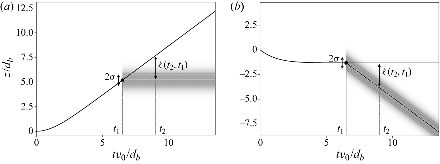
where  $\boldsymbol {\ell }_{adv}(t,s) = \int _s^{t} \tilde {\boldsymbol {u}}_{f,b} {(\boldsymbol {x}=\boldsymbol {x}_b(s^{{\dagger} }),s^{{\dagger} })}\,\textrm {d} s^{{\dagger} }$. Figure 2 is a space–time diagram that illustrates the integral formulation (2.24) and its Galilean invariance. The velocity disturbance at a given position and time is obtained from the summation over all the previous times of the momentum supplied by the bubble to the material point of the liquid that is at this specific position.
Space–time diagram of the evolution of the bubble position (solid black line) and that of the material point at which momentum has been disposed at  $t=t_1$ (black dashed line). (a) In the case of a steady carrier flow
 $\tilde {\boldsymbol {u}}_{f,b} {(\boldsymbol {x}=\boldsymbol {x}_b(t),t)}= 0$; (b) in the case of a uniform advection by the carrier flow
 $\tilde {\boldsymbol {u}}_{f,b} {(\boldsymbol {x}=\boldsymbol {x}_b(t),t)}=-v_0 \boldsymbol {e}_z$, with
 $\boldsymbol {e}_z$ the vertical direction. Galilean invariance imposes length preservation as shown in both cases by the distance
 $\ell (t_1,t_2)$. The shaded area represents the region of the flow influenced by the momentum disposed at
 $t=t_1$.

Note that the field  $\boldsymbol {u}^{*}_{f,b}$ is not divergence free. Although the effect of pressure can be taken into account in a similar way as was done by Gualtieri et al. (Reference Gualtieri, Picano, Sardina and Casciola2015), the formulation proposed in (2.24) has the advantage of being simpler and allows us to analytically compute the integrals in the case of an isolated bubble, as shown in the next section. Moreover, since the determination of the correct hydrodynamic force only requires the values of the velocity correction and its derivatives at the bubble position, the divergence of
 $\boldsymbol {u}^{*}_{f,b}$ does not appear as a serious issue. Finally, we consider that the fluid does not reside for a long time in the region of size
 $\sigma$ around a bubble and thus propose to simply evaluate
 $\boldsymbol {\ell }_{adv}(t,s)$ as
 \begin{equation} \boldsymbol{\ell}_{adv}(t,s) \approx \tilde{\boldsymbol{u}}_{f,b} {(\boldsymbol{x}=\boldsymbol{x}_b(t),t)} \times (t-s). \end{equation}
In § 3, we propose an efficient algorithm to compute the integral in (2.24) from the particle path history. Knowing  $\boldsymbol {u}^{*}_{f,b}$, it is then possible to evaluate the hydrodynamic forces involved in (2.11). The fluid velocity seen by the bubble is simply obtained by the difference between
 $\boldsymbol {u}_f$ and
 $\boldsymbol {u}^{*}_{f,b}$ as expressed by (2.13), while the corresponding fluid material derivative is given by
 \begin{equation} \left.\frac{\textrm{D} \left( \boldsymbol{u}_f - \boldsymbol{u}^{*}_{f,b} \right) }{\textrm{D} t} \right|_{\substack{\boldsymbol{x}_b(t)}} = \frac{\partial \boldsymbol{u}_f}{ \partial t} + \boldsymbol{u}_f \boldsymbol{\cdot}\boldsymbol{\nabla} \boldsymbol{u}_f - \frac{\partial \boldsymbol{u}^{*}_{f,b}}{ \partial t} - \boldsymbol{u}^{*}_{f,b} \boldsymbol{\cdot}\boldsymbol{\nabla} \boldsymbol{u}^{*}_{f,b}.\end{equation}
It is worth mentioning that no cross-term between  $\boldsymbol {u}_f$ and
 $\boldsymbol {u}^{*}_{f,b}$ is involved in (2.26) despite the nonlinear nature of the material derivative. The reason is that such terms must cancel to preserve the Galilean invariance of the added-mass force. The temporal and spatial derivatives of
 $\boldsymbol {u}^{*}_{f,b}$ can be easily computed by applying their definition to (2.24):
 \begin{align} \frac{\partial }{\partial t} \boldsymbol{u}^{*}_{f,b}{(\boldsymbol{x},t)} &= \frac{\boldsymbol{u}^{*}_{f,b} {\left(\boldsymbol{x}, t \right)} - \boldsymbol{u}^{*}_{f,b} {\left( \boldsymbol{x}, t-{\rm \Delta} t \right)} }{{\rm \Delta} t} \nonumber\\ &= \frac{1}{{\rm \Delta} t} \frac{1}{\rho_f} \int_{t-{\rm \Delta} t}^{t} \boldsymbol{F}_{b\rightarrow f}{\scriptstyle (s)} G_{\sigma}{\left(\boldsymbol{x} - \boldsymbol{x}_b(s) + \ell_{{adv}}(t-s)\right) }\,\textrm{d} s \nonumber\\ &= \frac{1}{\rho_f} \boldsymbol{F}_{b\rightarrow f}{(t)} G_{\sigma} {\left(\boldsymbol{x} - \boldsymbol{x}_b(t) \right)} \end{align}
and
 \begin{equation} \boldsymbol{\nabla} \boldsymbol{u}^{*}_{f,b}{(\boldsymbol{x},t)} = \frac{1}{\rho_f}\int_{t_0}^{t} \boldsymbol{F}_{b\rightarrow f}{(s)} \boldsymbol{\nabla} G_{\sigma} {\left(\boldsymbol{x}-\boldsymbol{x}_b(s)+\ell_{adv}(t-s)\right)} \,\textrm{d} s + \boldsymbol{\nabla}\boldsymbol{u}^{*}_{f,b} {(\boldsymbol{x},t_0)}, \end{equation}
where  $\boldsymbol {\nabla } G_{\sigma }$ is the gradient of the homogenization kernel, which is analytically known for a Gaussian kernel.
3. Numerical details and choice of parameters
In the following, we present numerical results obtained by integrating the coupled sets of equations, (2.4)–(2.7), (2.11)–(2.13), (2.24)–(2.28), which have been implemented in the numerical code already used by Zamansky et al. (Reference Zamansky, Coletti, Massot and Mani2016), Gorokhovski & Zamansky (Reference Gorokhovski and Zamansky2018), Bos & Zamansky (Reference Bos and Zamansky2019) and Zhang, Legendre & Zamansky (Reference Zhang, Legendre and Zamansky2019). The differential equations for the continuous phase (2.4)–(2.5) are solved with a pseudospectral method based on the P3DFFT library (Pekurovsky Reference Pekurovsky2012) with dealiasing of quadratic nonlinear terms by the  $2/3$ rule (Orszag Reference Orszag1971; Canuto et al. Reference Canuto, Hussaini, Quarteroni and Zang1988). The time integration of these equations is performed with the second-order Adams–Bashforth scheme.
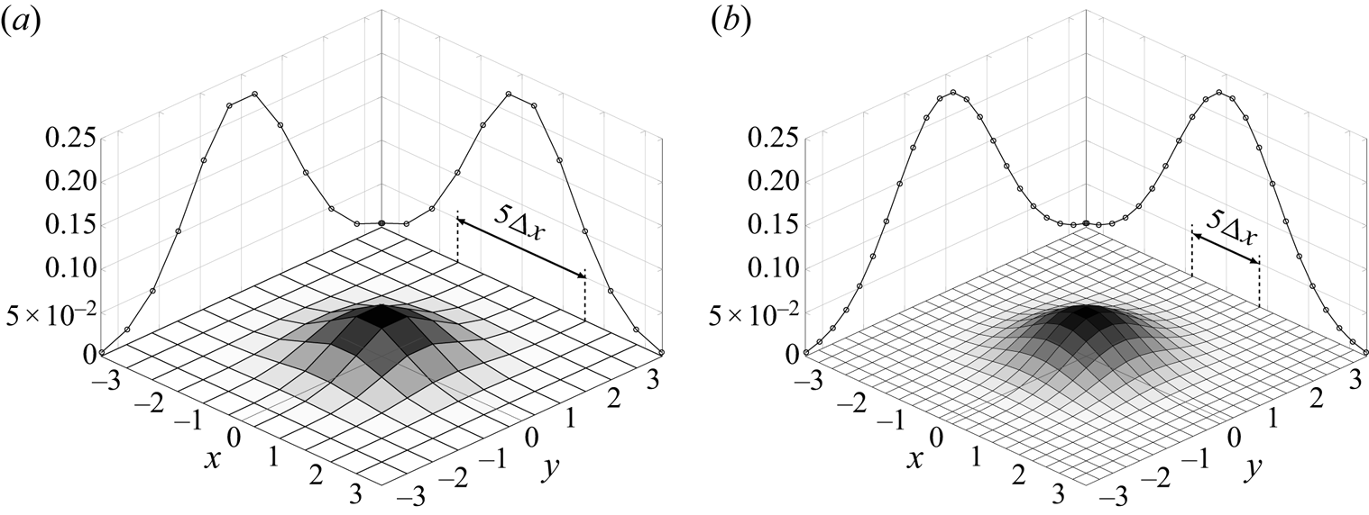
The differential equation for the dispersed phase (2.11) is also integrated with the Adams–Bashforth scheme with the same time step as for the integration of the continuous phase. The interpolations of the liquid velocity  $\boldsymbol {u}_f$ at the bubble positions are obtained by means of fourth-order splines (Yeung & Pope Reference Yeung and Pope1988). The projection on the Eulerian mesh of the momentum sources modelling the dispersed phase in (2.6) is carried out thanks to a discretized Gaussian kernel (see figure 3):
 \begin{equation} G_\sigma(\boldsymbol{x}_i, \boldsymbol{x}_b) = A \exp\left( (\boldsymbol{x}_i - \boldsymbol{x}_b)^{2}/2 \sigma^{2} \right), \end{equation}
where  $\boldsymbol {x}_i$ is the coordinate of the
 $i^{th}$ computational node and
 $A = {\rm \Delta} x^{-3} \sum _i \exp ( (\boldsymbol {x}_i - \boldsymbol {x}_b)^{2}/2 \sigma ^{2} )$, with
 ${\rm \Delta} x$ the grid spacing, is a normalization constant ensuring that the integral of the kernel is equal to one. In the next section, we will discuss how the value of
 $\sigma$ is determined.
Illustration of the Gaussian kernel used to distribute the Lagrangian quantities on the mesh grid. (a) A coarse mesh with  $\sigma /{\rm \Delta} x = 1.8$, (b) a finer mesh with
 $\sigma /{\rm \Delta} x = 3.7$.

We now present the details of the numerical implementation of the model that is used to cancel the self-induced force. We substitute in (2.24) and (2.27)–(2.28) the kernel width  $\sigma$ by
 $\sigma ^{*} = c_0 \sigma$, to account for the fact that a continuous kernel is involved in these calculations, while the Lagrangian to Eulerian projection kernel used to compute the momentum transfer from the bubble to the liquid is discrete. The velocity disturbance, its gradient and time derivative are then determined by
 $$\begin{gather} \boldsymbol{u}^{*}_{f,b}{(\boldsymbol{x}_b(t),t)} = c_1 \frac{1}{\rho_f} \int_{t_0}^{t} \boldsymbol{F}_{b\rightarrow f}{(s)} G_{\sigma^{*}}{(\boldsymbol{x}_b(t)-\boldsymbol{x}_b(s) + \boldsymbol{\ell}_{adv}(t,s) )}\,\textrm{d} s, \end{gather}$$
 $$\begin{gather}\boldsymbol{\nabla} \boldsymbol{u}^{*}_{f,b}{(\boldsymbol{x}_b(t), t)} = c_2 \frac{1}{\rho_f}\int_{t_0}^{t} \boldsymbol{F}_{b\rightarrow f}{(s)} \boldsymbol{\nabla} G_{\sigma_*}{\left(\boldsymbol{x}_b{(t)}-\boldsymbol{x}_b(s)+\ell_{adv}(t-s)\right)}\,\textrm{d} s. \end{gather}$$
 $$\begin{gather}\frac{\partial }{\partial t} \boldsymbol{u}^{*}_b{(\boldsymbol{x}_b(t),t)} = c_3 \frac{1}{\rho_f} \boldsymbol{F}_{b\rightarrow f}{(t)} G_{\sigma_*} {\left(\boldsymbol{x}_b{(t)}-\boldsymbol{x}_b(t-dt)+\ell_{adv}(dt)\right)}, \end{gather}$$
where the prefactors  $c_1$,
 $c_2$ and
 $c_3$ are introduced consistently with the change of kernel width. In the next section, we will detail the procedure to determine the value of these parameters, but it is important to bear in mind that parameters
 $c_1$,
 $c_2$ and
 $c_3$ can all be expressed from
 $c_0$ only. The latter is thus the only free parameter, which depends on
 $\sigma /{\rm \Delta} x$ and on the chosen numerical schemes.
The integrals involved in (3.2) and (3.3) are estimated by means of the trapezoidal method. To compute their value at a given instant, the coordinates of the bubble positions and the strength of the momentum sources need to be known at previous times. The integrand  $\delta \boldsymbol {u}^{*}_{f,b}(t,s) = \boldsymbol {F}_{b\rightarrow f}{(s)} G_{\sigma ^{*}}{(\boldsymbol {x}_b(t)-\boldsymbol {x}_b(s) + \boldsymbol {\ell }_{adv}(t,s) )}$ vanishes for time lags such that the distance in the argument of the kernel
 $G_{\sigma }$ is large:
 $\boldsymbol {x}_b(t)-\boldsymbol {x}_b(s) + \boldsymbol {\ell }_{adv}(t,s) \gg \sigma$. Therefore, the integral should converge for
 $t_0 \ll t - \sigma / | \tilde {\boldsymbol {u}}_{f,b} - \boldsymbol {v}_b|$, where
 $| \tilde {\boldsymbol {u}}_{f,b} - \boldsymbol {v}_b|$ characterizes the velocity of the bubble relative to the liquid. It is therefore necessary to keep track of the bubble-path history over the last
 $N_h = (t-t_0)/d t$ time steps of the numerical simulation (with
 $d t$ the time increment). However, depending on
 $\sigma /{\rm \Delta} x$ and on
 $d t$, the number
 $N_h$ of instants to be kept in memory can be quite large, therefore requiring significant CPU time and computer memory. In the simulations presented below,
 $N_h$ is typically 600. To efficiently perform the integrations, we propose not to keep in memory all previous instants between
 $t$ and
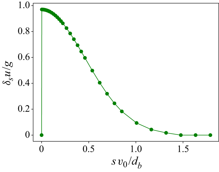
 $t_0$. This is illustrated in figure 4, which shows the evolution of the integrand in (3.2) as a function of
 $s$ for the case a single rising bubble that will be presented in the next section. In this figure, the uneven recorded instants are denoted by dot symbols. The first few instants of the history, where the integrand changes rapidly, are updated every time step, whereas as we go further back in the past, the list of previous positions and momentum sources is updated less frequently. The details of this algorithm are given in Appendix B. The integral computed with this algorithm is very accurate and, in the meantime, enables us to save significant computer resources, since it requires to store only approximately 30 instants of the path history of each bubble.
Evolution of the integrand  $\delta _s\boldsymbol {u}(t,s) = \boldsymbol {F}_{b\rightarrow f}{\scriptstyle (s)} G_{\sigma ^{*}}{\scriptstyle (\boldsymbol {x}_b(t)-\boldsymbol {x}_b(s) + \boldsymbol {\ell }_{adv}(t,s))}$ in (3.2) as a function of
 $s$ for the case of a single rising bubble. The instants that are used to compute the integral are denoted by the dot symbols. We note their uneven distribution, with a large density for recent times and a small density at large time lag.

From this point on, the density  $\rho _b$ of the dispersed phase will be set to zero, which is equivalent to neglecting the density of the gas relative to that of the liquid.
3.1. A single bubble rising in an unbounded liquid at rest
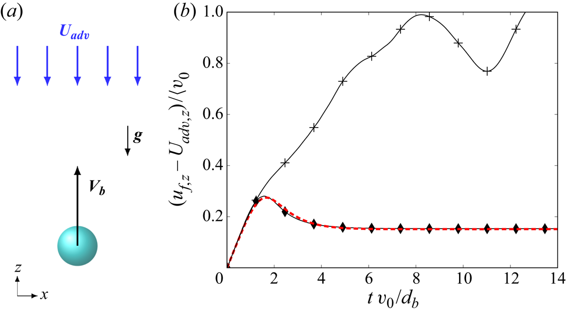
We now consider the case of a single bubble rising in a liquid otherwise at rest. This simple case has the great advantage that the undisturbed fluid velocity field is trivially zero ( $\tilde {\boldsymbol {u}}_b=0$) since, in the absence of the bubble, the liquid would stay at rest. First, values of the bubble drag coefficient
 $C_D$ and of the kernel width
 $\sigma$ leading to realistic simulated wakes are estimated from comparisons with experimental results. Then, we present a first validation of the method to compute the hydrodynamic force by verifying that the undisturbed liquid velocity and acceleration provided by the model (2.24) remain zero, i.e.
 $\boldsymbol {u}^{*}_{f,b}=\boldsymbol {u}_{f}$.
Since  $\tilde {\boldsymbol {u}}_b=0$, (2.11) simplifies and the vertical bubble velocity evolves as
 \begin{equation} \frac{\textrm{d} v_{b,z}}{\textrm{d} t} = \frac{3}{4} \frac{C_D}{C_M} \frac{v_{b,z}^{2} }{d_b} - \frac{g}{C_M}, \end{equation}
where  $\boldsymbol {g} = -g \boldsymbol {e}_z$. In general, the added-mass coefficient of a bubble depends on its shape while the drag coefficient depends both the shape and the Reynolds number (Moore Reference Moore1965; Ishii & Zuber Reference Ishii and Zuber1979; Maxworthy et al. Reference Maxworthy, Gnann, Kürten and Durst1996). In this study, we choose the value of the drag coefficient to be consistent with the average rising speed of the experiments of Ellingsen & Risso (Reference Ellingsen and Risso2001) and Riboux et al. (Reference Riboux, Risso and Legendre2010). In their experiments, an air bubble with a diameter
 $d_b=2.5$ mm rises in water at an average speed of
 $v_0=0.305$ m s
 $^{-1}$, which corresponds to a bubble Reynolds number
 $Re_b = v_0 d_b /\nu \approx 760$ and an average drag coefficient
 \begin{equation} C_D = \frac{4}{3} g \frac{d_b}{v_{0}^{2}} \approx 0.35. \end{equation}
When many bubbles are present, their interactions make their velocities fluctuate and cause their drag coefficients to increase. There have been several attempts to determine the drag coefficient in a bubble swarm. In particular, Akiki, Jackson & Balachandar (Reference Akiki, Jackson and Balachandar2017) recently proposed a numerical procedure to account for the dependence of  $C_D$ on the flow configuration and particle distribution. In the present large-scale simulations, we focus on the fluctuations resulting from wake interactions, which are expected to weakly depend on the details of the flow at the bubble scale. For this reason, we will not consider the variations of the drag coefficient associated with the presence of the other bubbles and we will adopt
 $C_D=0.35$ for our subsequent simulations of a rising bubbles swarm. Similarly, we will fix the added-mass coefficient
 $C_M$ to the value 1/2 corresponding to a sphere, thereby neglecting the variations of shapes and orientations of the bubbles, which would require the introduction of an anisotropic added-mass tensor.
In the experiment of Ellingsen & Risso (Reference Ellingsen and Risso2001), the fluid velocity in the wake of an isolated bubble has been measured. We can thus adjust the value of the kernel width  $\sigma$ for a given mesh resolution so as to reproduce the experimental bubble wake. According to (2.12), the momentum forcing transferred to the liquid by a single rising bubble can be expressed as
 \begin{equation} \boldsymbol{F}_{b \rightarrow f} ={-}\mathcal{V}_b \rho_{f} \boldsymbol{g} = F_0 \boldsymbol{e_z}. \end{equation}
Also, the bubble trajectory is known analytically from (3.5). Therefore, we can integrate the Navier–Stokes equations (2.4)–(2.5) to compute the fluid velocity induced by the rising of a single bubble, without explicitly considering the coupling with the dispersed phase. For such a simulation with a prescribed bubble motion, two numerical parameters need to be set: the grid spacing  ${\rm \Delta} x$ and the width
 $\sigma$ of the Gaussian kernel. (Note that we only consider here a uniform mesh with the same spacing in the three directions.)
Several simulations have been performed to analyse the influence of these parameters upon the induced-velocity field. In any case, the computational domain is a parallelepiped of dimensions  $L_x=L_y$ and
 $L_z$, with periodic boundary conditions in all three directions. The domain height
 $L_z$ is set such that a bubble reaches its terminal velocity and travels about 125 times its diameter before meeting its own wake because of the domain periodicity. Since the wake vanishes very slowly, it would require a longer box for a bubble not to interact at all with its own wake and a truly stationary state to be observed, which indicates that interactions between bubbles are expected to occur even at very small volume fractions. We consider 5 different mesh resolutions ranging from
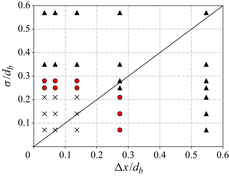
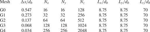
 ${\rm \Delta} x / d_b = 0.55$ to 0.034. The details of the computational grids are given in table 1. For each of these grids, we have tested 7 values of
 $\sigma$ ranging from
 $0.071 d_b$ to
 $0.57 d_b$, as summarized in the parameter map of figure 5. For all simulations, the bubble diameter, the kinematic viscosity and the gravity are kept constant as respectively
 $d_b=2.5$ mm,
 $\nu = 10^{-6}$ m
 $^{2}$ s and
 $g=9.81$ m s
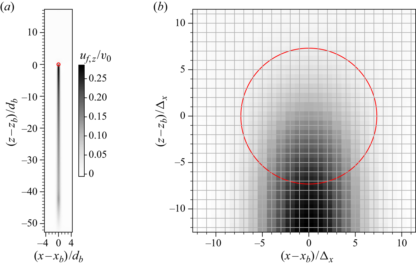
 $^{-2}$. The resulting wake is illustrated in figure 6. To determine the appropriate value of
 $\sigma /d_b$ for a given value of
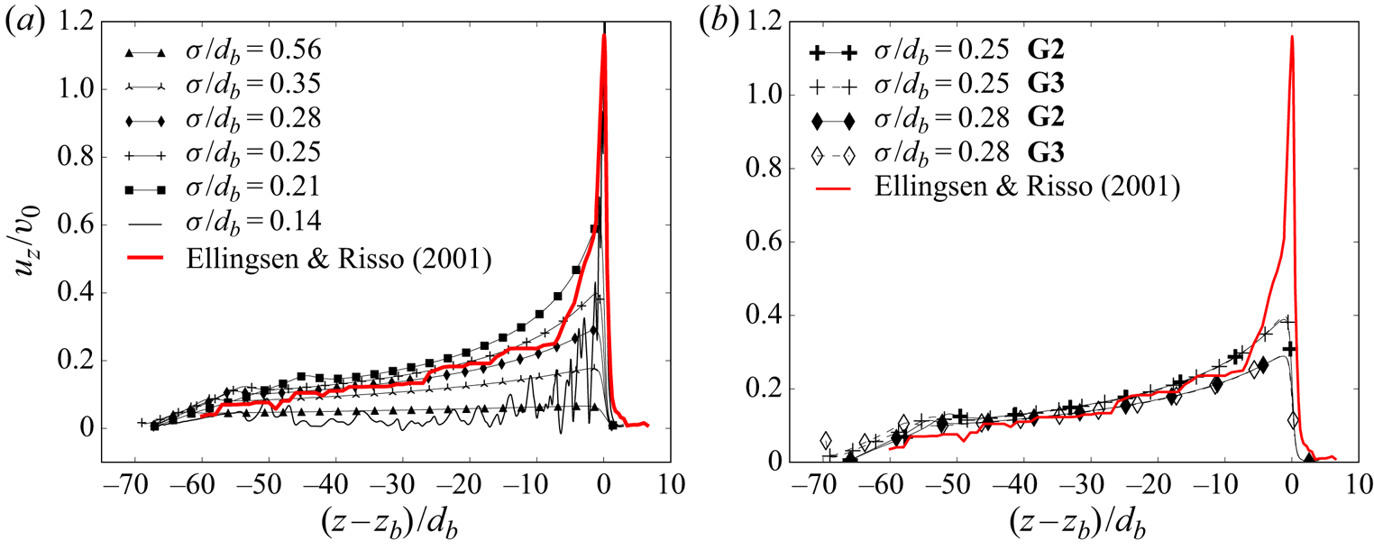
 ${\rm \Delta} x/d_b$, we compare the vertical fluid velocity along a vertical axis passing through the centre of the bubble with the measurement of Ellingsen & Risso (Reference Ellingsen and Risso2001). This spatial evolution of the fluid velocity is shown in figure 7 for
 ${\rm \Delta} x/d_b=0.068$ (mesh G3). It is clearly seen that the value of
 $\sigma /d_b$ strongly influences the results of the numerical simulations. Owing to the self-similarity property of the wakes, we expect that for distances far enough away from the bubble, the wake depends only on the bubble Reynolds number and is no longer influenced by the details of the momentum source. In the near-bubble region, a smaller kernel width will result in a better prediction by the numerical model. It is indeed observed that for large
 $\sigma$, the fluid velocity is underestimated compared with the experiment, because, in that case, the momentum source is spread over too large a region, while with small values of
 $\sigma$, the velocity peak in the vicinity of the bubble tends to be well reproduced. Nevertheless, we observe the apparition of instabilities for
 $\sigma /d_b<0.2$, which are visible in figure 7 and probably caused by too high a momentum source density, which leads to a fluid velocity at the bubble position that is larger than the bubble velocity. It is worth mentioning that the features of this instability, when it develops, do not depend on the mesh-size spacing or on the time step. Similar trends regarding the influence of
 $\sigma$ on the wake, not reported here, are also observed for the other mesh resolutions. In particular, we observe that when
 $\sigma$ is smaller than the grid spacing, the entire momentum source is contained in a single computational cell (as in the ‘particle-in-cell’ approach) and there is thus no more effect of further reducing
 $\sigma$. To summarize, we observe the best agreement between the numerical simulations and the experiments for
 $\sigma /d_b \approx 0.25$ with grids G2, G3 and G4, while for grid G1 the wake is better reproduced with
 $\sigma /d_b \approx 0.21$. Figure 7(b) compares these settings. No difference is observed between the results obtained with meshes G2 and G3, which indicates that grid convergence can be reached.
Map of the parameters  ${\rm \Delta} x/d_b$ and
 $\sigma /d_b$ considered for the simulations of the single rising bubble. The circles denote cases in which the wake is well reproduced and the model for the disturbance gives accurate estimations, whereas triangles indicate cases where the wake is poorly described due to a lack of resolution, and crosses correspond to unstable simulations.

Illustration of the liquid vertical velocity field  $u_{f,b}$ in a
 $x$–
 $z$ plane passing through the bubble centre for the simulation with grid G3 (
 ${\rm \Delta} x/d_b = 0.068$) and
 $\sigma /d_b=0.24$. (a) View of the full numerical domain, (b) zoom-in close to the bubble. The bubble is represented by the red circle.

Vertical velocity of the fluid in the wake of the bubble normalized by the terminal velocity of the bubble: (a) for different values of  $\sigma /d_b$ and mesh G3. Red line, experimental result of Ellingsen & Risso (Reference Ellingsen and Risso2001); black symbols, numerical results for various values of
 $\sigma /d_b$; (b) for grids G2 and G3, and
 $\sigma /d_b= 0.24$ and 0.28.

Characteristics of the different computational grids for the test of a single rising bubble. In all simulations the bubble diameter, the kinematic viscosity and the gravity are kept constant as respectively  $d_b=2.5$ mm,
 $\nu = 10^{-6}$ m
 $^{2}$ s
 $^{-1}$ and
 $g=9.81$ m s
 $^{-2}$.

We now focus on the validation of our model for the disturbed fluid velocity. The simulations just mentioned above, for which the bubble trajectory and momentum forcing were imposed from (3.5) and (3.7), give the reference liquid velocity disturbance, since the undisturbed velocity was identically zero. This reference is used to determine the constants of our model in (3.2), (3.3) and (3.4) as follows. Once the velocity of the bubble is stationary, (3.2)–(3.4) can be evaluated analytically, which leads to relate  $c_1$,
 $c_2$ and
 $c_3$ to
 $c_0$ by
 $$\begin{gather} c_1 = u^{*}_{f,b,z} \frac{ 4{\rm \pi} \sigma^{2} c_0^{2} v_0 }{F_0/\rho_f}, \end{gather}$$
 $$\begin{gather}c_2 ={-} \partial_z u^{*}_{f,b,z} \frac{(2{\rm \pi} \sigma^{2} c_0^{2})^{3/2} v_0 } {F_0/\rho_f}, \end{gather}$$
 $$\begin{gather}c_3 = \partial_t u^{*}_{f,b,z} \frac{(2{\rm \pi} \sigma^{2} c_0^{2} )^{3/2}} {F_0/\rho_f}, \end{gather}$$
where the values of the liquid velocity disturbance and its derivatives at the bubble centre,  $u^{*}_{fb,z}$,
 $\partial _z u^{*}_{f,b,z}$ and
 $\partial _t u^{*}_{f,b,z}$, are taken from the uncoupled simulation, in order to have
 $\boldsymbol {u}_{f} = \boldsymbol {u}^{*}_{f,b}$.
Then, the performance of our model is evaluated by comparing its prediction to the reference simulation. In figure 8(a), we examine the fluid vertical velocity at the bubble position for grid G2 and  $\sigma /d_b=0.25$. In this case the value of
 $c_0$ has been adjusted to 1.62 by least-square fitting between the reference simulation and (3.2), which leads to the other parameters being
 $c_1=2.88$,
 $c_2=1.17$ and
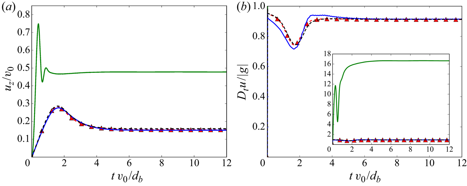
 $c_3=1.17$ by using (3.8)–(3.10). We present the temporal evolution of the actual fluid velocity at the bubble position, as well as the velocity disturbance computed from the bubble path history according to (3.2). It is seen that both curves overlap very well, which indicates that the undisturbed velocity is indeed zero. Moreover, the comparison with the reference simulation is also very good, which provides a first validation of the model used to calculate the disturbance. In figure 8(b), we show a similar comparison for the vertical component of the total fluid acceleration. It is seen as well that the fluid acceleration at the bubble position is nearly equal to the computed acceleration disturbance and to the reference fluid acceleration at the bubble position. The undisturbed fluid acceleration is thus zero and we can conclude that the perturbed acceleration is accurately computed. It should be noted that, for
 $\sigma /d_b \leq 0.21$, the velocity and acceleration disturbances show some deviation compared with the reference values.
Temporal evolution of the fluid vertical velocity at the bubble position normalized by the bubble terminal velocity (a) and the fluid vertical acceleration at the bubble position normalized by gravity (b). Red triangles, results of the reference simulation with prescribed momentum source; blue lines, results from the full simulation including the correction of the hydrodynamic force; black dashed lines, velocity or acceleration disturbance given by the model implemented in the full simulation; green lines, results of the full simulation without accounting for the correction of the hydrodynamic force ( $\boldsymbol {u}^{*}_{f,b} = 0$). These tests have been carried out with grid G2 (
 ${\rm \Delta} x / d_b = 0.14$) and
 $\sigma /d_b=0.28$. The inset of panel (b) is a zoom-out that shows uncorrected results.

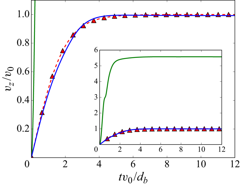
Since the unperturbed fluid velocity and acceleration are accurately predicted, the hydrodynamic force on the bubble can also be accurately computed. This is confirmed by figure 9, which compares the reference analytical evolution of the bubble velocity obtained from (3.5) with the evolution obtained from the simulation of the full set of coupled equations. The analytical and simulated bubble velocities are very close to each other, which validates the proposed method to cancel the spurious self-induced force. To emphasize the importance of this correction in the case of a single bubble rising at large Reynolds number, figures 8 and 9 also show the results of the coupled simulation obtained without accounting for the correction of the liquid velocity at the bubble location, i.e. by setting  $\boldsymbol {u}^{*}_{f,b}=0$. Without correction, the computed values are indeed largely off from the reference values and can even further lead to the divergence of the numerical simulation.
Vertical velocity of the bubble normalized by its terminal velocity. Red triangles, reference case ( $\tilde {\boldsymbol {u}}_{f,b}=0$); green line, case without correction (
 $\tilde {\boldsymbol {u}}_{f,b}=\boldsymbol {u}_f$); blue line, results accounting for the correction (
 $\tilde {\boldsymbol {u}}_{f,b} = \boldsymbol {u}_f - \boldsymbol {u}^{*}_{f,b}$). The inset is a zoom-out that shows the uncorrected results.

Now, it is useful to estimate when the correction of the spurious self-induced force is required. When  $| \tilde {\boldsymbol {u}}_{f,b} - \boldsymbol {v}_b| \gg |\boldsymbol {u}^{*}_{f,b}|$, the velocity disturbance has a negligible effect on the drag force. Additionally, when
 $| D_t \tilde {\boldsymbol {u}}_{f,b} - d_t \boldsymbol {v}_b| \gg | D_t \boldsymbol {u}^{*}_{f,b}|$, the effect on the forces resulting from the liquid inertia is negligible. These inequalities can easily be tested a posteriori, from the knowledge of the bubble path and with the help of the proposed model for
 $\boldsymbol {u}^{*}_{f,b}$. They can be also be estimated a priori by assuming that the momentum exchange in (2.12) is only due to the drag force (which is exact in the case for a single rising bubble at stationary state and approximate for a bubble in a bubble swarm) and by considering that the integrand in (2.24) is non-negligible only over time of the order of
 $\sigma / | \tilde {\boldsymbol {u}}_{f,b} - \boldsymbol {v}_b|$ (see figure 2). This leads to the following scaling for the ratio of the velocity disturbance to the relative velocity between the bubble and the liquid:
 \begin{equation} \frac{|\boldsymbol{u}^{*}_{f,b}| }{ | \tilde{\boldsymbol{u}}_{f,b} - \boldsymbol{v}_b|} \sim C_D \frac {d_b^{2}}{\sigma^{2}}. \end{equation}
From (3.11), we conclude that it is essential to correct the fluid velocity for large-Reynolds-number bubbles, since, in this case,  $C_D = O(1)$ and
 $\sigma /d_b = O(1)$. Note that for objects moving at small Reynolds number, an estimate obtained from the averaging of the Stokeslet (2.17) gives
 $|\boldsymbol {u}^{*}_{f,b}| / | \tilde {\boldsymbol {u}}_{f,b} - \boldsymbol {v}_b| = O(d_b/{\rm \Delta} x)$ (Saffman Reference Saffman1973; Boivin et al. Reference Boivin, Simonin and Squires1998), which means that the correction can be disregarded for sufficiently small objects and coarse description of the velocity field.
It is worth noting that even if coupling between the two phases through the hydrodynamic force acting on the bubbles and the transfer of momentum to the liquid by diffused sources ensure the conservation of momentum for the mixture, it does not conserve its energy (Xu & Subramaniam Reference Xu and Subramaniam2007; Subramaniam et al. Reference Subramaniam, Mehrabadi, Horwitz and Mani2014). Indeed, the power  $P_b$ of the hydrodynamic force working at the bubble velocity is larger than the power
 $P_f$ of the diffused force working at the fluid velocity:
 \begin{equation} P_b=\sum_b \boldsymbol{F}_{b\rightarrow f }\cdot \boldsymbol{v}_b > P_f=\int {\textrm{d}{\kern 0.2em}x}^{3} \boldsymbol{f}\cdot\boldsymbol{u}_f. \end{equation}
However, it is physically acceptable that a certain amount of energy is dissipated within the interphase coupling, since we consider a coarse-grained description of the continuous phase, in which the strong velocity gradients in the vicinity of the bubbles are not resolved. In other words, the dissipation of kinetic energy into heat that occurs in the region surrounding the bubble at scales smaller than  $\sigma$ cannot be computed from
 $\boldsymbol {u}_f$.
Nevertheless, the energy dissipated in the coupling can be estimated from the model for the perturbed velocity  $\boldsymbol {u}^{*}_{f,b}$. Let us do this for the case of the isolated bubble. From (2.6), (2.24) and (3.7), and considering
 $\boldsymbol {u}_f=\boldsymbol {u}^{*}_{f,b}$, we obtain
 \begin{equation} P_f = \frac{F_0^{2}}{\rho_f} \int G_{\sigma}( \boldsymbol{x}-\boldsymbol{x}_b(t)) \int_{-\infty}^{t} G_{\sigma}( \boldsymbol{x}-\boldsymbol{x}_b(s))\,\textrm{d} s {\textrm{d}{\kern 0.2em}x}^{3}. \end{equation}
By introducing the non-dimensional variables  $\boldsymbol {\chi } = (\boldsymbol {x}-\boldsymbol {x}_b(t)) / \sigma$ and
 $\tau = (t-s) v_0/\sigma$, we get
 \begin{equation} P_f = \frac{F_0^{2}}{\rho_f \sigma^{2} v_0} \underbrace{\int \int_{0}^{\infty} G_{1}( \boldsymbol{\chi} ) G_{1}( \boldsymbol{\chi} + \tau\boldsymbol{e}_z )\,\textrm{d}\tau\,\textrm{d}\chi^{3} }_{k}, \end{equation}
with  $\boldsymbol {e}_z$ the vertical direction. Owing to
 $G$ being a Gaussian kernel, the summation can be evaluated analytically and gives
 $k=1/8{\rm \pi}$. It should be remarked that if we account for the numerical parameters in the computation of the velocity perturbation (that is to say, taking (3.2) instead of (2.24)), we get
 $k=c_1/c_0^{2} 8{\rm \pi}$. Since the energy given by the bubble is
 $P_b = F_0 v_0$, we have
 \begin{equation} \frac{P_f}{P_b} = \frac{C_D }{64} \left( \frac{d_b}{\sigma}\right)^{2}. \end{equation}
For  $C_D=0.35$ and
 $\sigma /d_b = 0.28$, this estimate leads to
 ${P_f}/{P_b} \approx 0.07$, which means that most of the mechanical energy that is exchanged between the bubble and the liquid is dissipated in the vicinity of the bubble.
In Appendix A, we present some tests showing that the proposed model respects Galilean invariance.
3.2. Repulsive force between bubbles
Since the sources of momentum that model the bubbles are spanned over a few mesh-grid steps, it is possible that two bubbles overlap when simulating multiple bubble trajectories. To prevent such a non-physical behaviour, we introduce an interaction force between bubbles that prevents them from overlapping. In the bubble momentum balance equation (2.11), the term  $\boldsymbol {F}_{{I},b}$ is expressed as
 \begin{equation} \boldsymbol{F}_{{I},b} = \sum_{b'\neq b} \boldsymbol{F}_{r_{b', b}}, \end{equation}
with
 \begin{equation} \boldsymbol{F}_{r_{b', b}} ={-} C_I \frac{\boldsymbol{x}_{b'}-\boldsymbol{x}_b }{r_{b', b}} \exp\left( - r_{b', b}^{2} / 2 r_{I}^{2} \right), \end{equation}
where  $r_{b', b}=| \boldsymbol {x}_{b'}-\boldsymbol {x}_b |$ is the distance between the centres of bubbles
 $b$ and
 $b'$. The range of the force is limited by setting
 $\boldsymbol {F}_{r_{b' \rightarrow b}} = 0$ for
 $r_{b', b} > 3 r_{I}$. The parameter
 $r_{I}$ is set as
 $d_b/2$ whereas
 $C_I$, which has a unit of force, is adjusted so that two rising bubbles reach an equilibrium distance
 $r_{b', b}$ equal to
 $d_b$. For grid G3 with
 ${\rm \Delta} x/d_b=0.068$ and
 $\sigma /d_b=0.28$, this corresponds to
 $C_I/(\rho _f {v_0}^{2} d^{2})=0.34$.
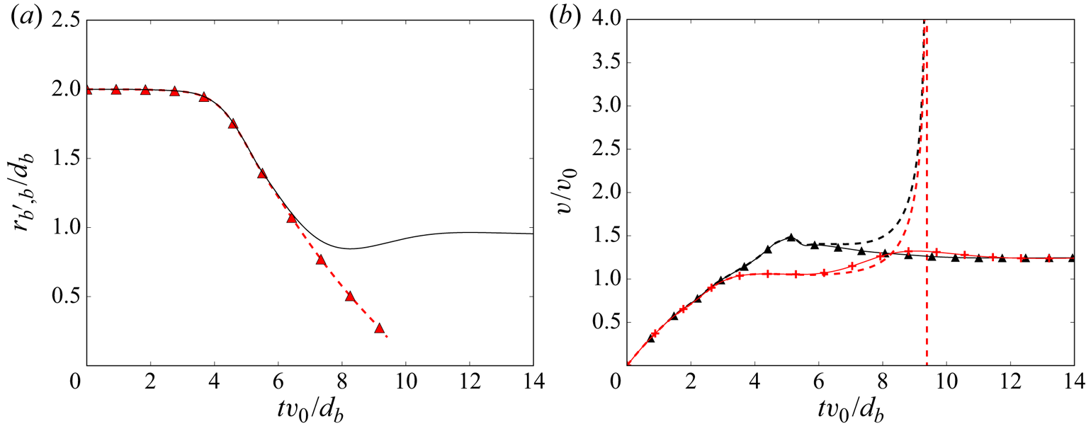
The effect of this force is illustrated in figure 10, which shows the temporal evolution of the positions of two vertically aligned rising bubbles. When the repulsive force is implemented, the distance between the bubble centres reaches a stationary value corresponding to  $r_{b', b}= d_b$ and the terminal velocity of the pair is approximately 30 % larger than that of a single bubble. The actual interaction between two rising bubbles is more complicated (van Wijngaarden Reference van Wijngaarden1993; Harper Reference Harper1997; Hallez & Legendre Reference Hallez and Legendre2011). However, our motivation to include this repulsive force is just to ensure numerical stability, since the bubble velocity can diverge when two bubbles are allowed to overlap.
(a) Temporal evolution of the distance between the two bubbles rising in line. Continuous black line, with repulsive force and dashed line with triangles, without repulsive force. (b) Temporal evolution of the vertical velocity of the two bubbles. The first bubble corresponds to the red curve, the second bubble corresponds to the black curve. Comparison of the cases with or without repulsive force shown respectively by the continuous lines with symbols and dashed lines.

4. Simulation of a bubble swarm and comparison with experiments
In this section, we present the results of large-scale numerical simulations of a swarm of bubbles rising at large Reynolds number, which are based on the Euler–Lagrange approach including our model to correct the spurious self-induced hydrodynamic force. A single set of physical parameters is considered:  $d_b=2.5\ \textrm {mm}$,
 $\nu =10^{-6}$ m
 $^{2}$ s
 $^{-1}$ and
 $g=9.81$ m s
 $^{-2}$. This corresponds to the experiments of Riboux et al. (Reference Riboux, Risso and Legendre2010), who investigated air bubbles that rise in water at a velocity of approximately 0.3 m s
 $^{-1}$ (
 $Re\approx 760$). In these experiments, a stable homogeneous bubble column with zero average liquid velocity is obtained thanks to a carefully designed bubble injection. In the simulations, the volume fraction is set to
 $\alpha = 2\,\%$ and the initialization is done with bubble and fluid velocities set to zero and a non-overlapping random distribution of bubbles within a cubic periodical domain of side width
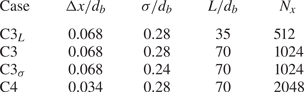
 $L$. Four simulations involving different numerical parameters are examined (see table 2). Simulation C3 is the reference case with a mesh resolution
 ${\rm \Delta} x / d_b=0.068$, a kernel width
 $\sigma /d_b=0.28$ and a domain size
 $L/d_b=70$. Each of the other cases differs from C3 by only one parameter. The domain size of case C3
 $_L$ is twice smaller, the kernel width of case C3
 $_\sigma$ is 15 % smaller and the mesh-grid spacing of case C4 is twice smaller.
Numerical parameters for the simulations of the bubble swarm.

A first important result is that, in all the present simulations, the bubble distribution remains homogeneous all along the computational time duration. This allows us to conclude that the model implemented to compute the bubble motions does not give birth to any instability of the homogeneous distribution of the bubbles in this range of physical parameters, in agreement with the experiments.
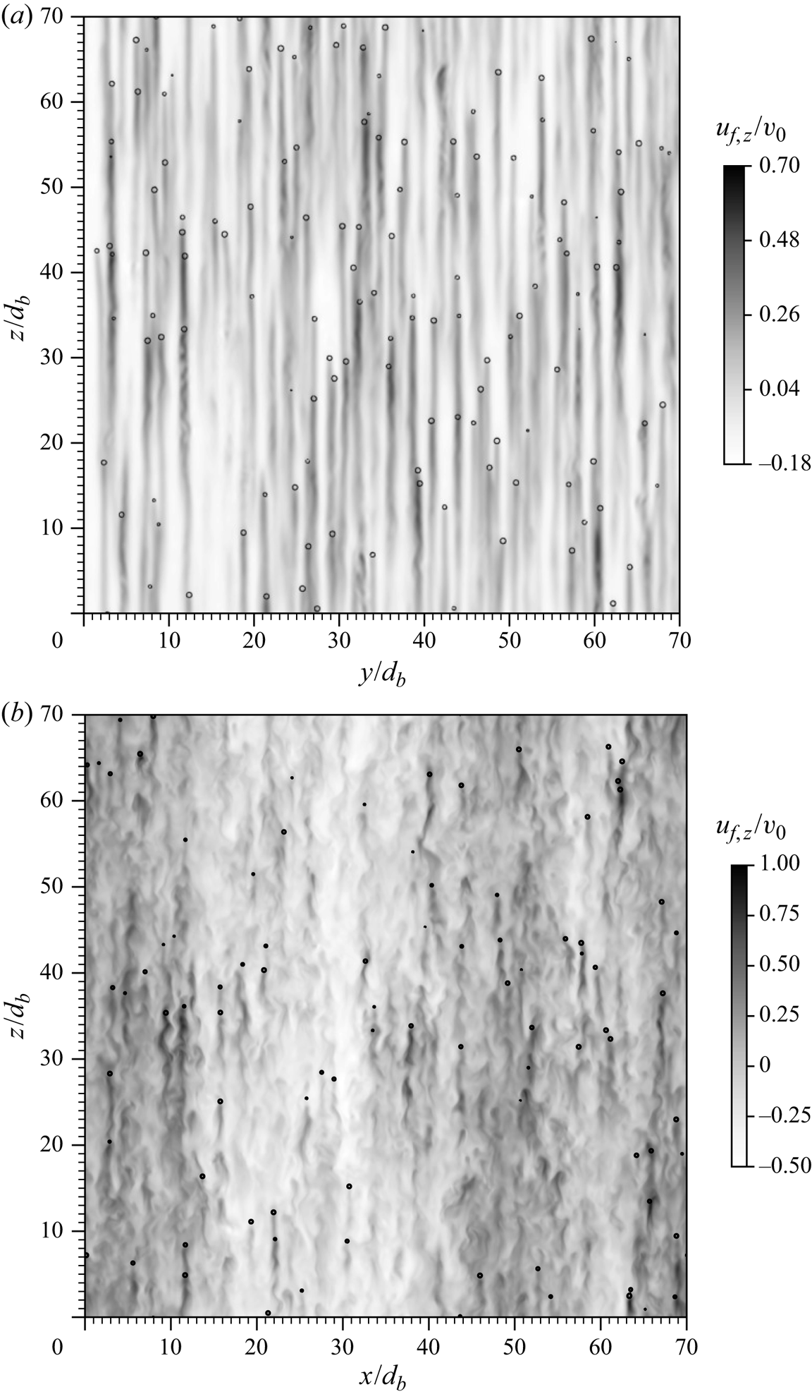
Figure 11 displays snapshots of the vertical liquid velocity corresponding to two different instants of case C3. The first is situated within the transient regime ( $t\approx 20 d_b/v_0$), just after the bubbles have completed their acceleration phase and reached their terminal velocity. Long almost-steady wakes have developed behind the bubbles while, outside those wakes, the liquid velocity is negligible. At this stage, the liquid velocity is thus dominated by the individual disturbances generated by the bubbles. The second snapshot corresponds to a later time lying in the final steady regime (
 $t\approx 2000 d_b/v_0$). Individual wakes are still visible but have been attenuated by interactions with their neighbours. In addition, turbulent fluctuations have developed. As observed in experiments, the liquid fluctuations in a homogeneous bubble swarm combine two contributions, the localized bubble disturbances (LBD) generated around each bubble and the bubble-induced turbulence (BIT), which is almost homogeneously distributed over all the domain (Risso Reference Risso2018).
Instantaneous vertical velocity of the liquid in a  $x$–
 $z$ plane at
 $t=20 d_b/v_0$ (a) and at
 $t=2000d_b/v_0$ (b) for a bubble swarm with
 $\alpha =2\,\%$ for case C3 (see table 2). The black circles show the bubble positions.

Figure 12 shows the time evolution of the fluid kinetic energy,  $K_f=\frac {1}{2} (\langle \boldsymbol {u}_x^{2}\rangle +\langle \boldsymbol {u}_y^{2}\rangle +\langle \boldsymbol {u}_z^{2}\rangle )$, and the viscous dissipation rate of energy within the fluid,
 $\epsilon$. In a first stage, the average bubble speed increases from zero until it reaches a maximum, before rapidly relaxing towards the terminal average speed. Bubble wakes develop as the bubbles accelerate, which entrain the fluid and cause
 $K_f$ to follow the same trend as
 $\langle v_z \rangle$. In the second stage of the transient,
 $K_f$ follows a more complex evolution as turbulent fluctuations develop. It first increases before decreasing back to almost the same value as that reached at the end of the first stage. Thus, although the final value of
 $K_f$ accounts for both wakes (LBD) and turbulence (BIT), it is similar to the value it reached before the onset of the first turbulent fluctuations, when only wakes were present. The examination of the dissipation rate leads to a deeper understanding of the process. In particular, it reaches a constant value as soon as the bubbles have reached their terminal speed, which means that, whatever the precise structure of the flow is, the dissipation is determined by the work of the buoyancy. Thus, because the power that is injected to the fluid is the same before and after the development of the turbulent fluctuations, the kinetic energy is the same as well, even if it is divided differently into LBD and BIT. Note also that, due to the coarse-graining procedure, the value of
 $\epsilon$ is much smaller than the work of the buoyancy on the bubbles from an amount,
 $\varepsilon / (\alpha g v_0) \approx 0.1$, which is in agreement with the estimate provided by (3.15).
Temporal evolution of the volume averaged turbulent kinetic energy (a) and of the volume averaged viscous dissipation (b) of the liquid caused by the rising bubbles for the case  $C3_L$ (see table 2).

Now, we analyse the effect of the numerical filtering of the small scales by considering the variances of the various components of the liquid velocity for the different simulated cases, which are given in table 3. In reference case C3, the simulation reproduced approximately 60 % of the vertical variance, 15 % of the horizontal variance and 30 % of the total kinetic energy. The fact that more energy is filtered in the horizontal direction is mainly due to the absence of wake-induced bubble path oscillations, which are able to redistribute fluctuating energy from the vertical component to the horizontal one, reducing the anisotropy of the fluctuations. The numerical parameters have some visible effects on the filtering of the liquid fluctuations, which are, however, not drastic from the perspective of the comparison with the experiments. As shown in § 3.1 from the analysis of the isolated bubble, reducing the kernel width leads to a better description of the large velocity fluctuations in the vicinity of the bubble. In the bubble swarm, we see that changing  $\sigma /d_b$ from 0.28 (case C3) to 0.24 (case C3
 $_\sigma$) has a rather small effect, as it leads to increase the vertical variance by only 4 % and the horizontal variance by 14 %. Refining the mesh grid by a ratio of two, spacing
 ${\rm \Delta} x$ from 0.68 (case C3) to 0.34 (case C4) results in 30 % increase in the vertical direction and less than 8 % increase in the horizontal direction. Decreasing the domain size from 70
 $d_b$ (case C3) to 35
 $d_b$ (case C3
 $_L$), increases the vertical variance by
 $12\,\%$ but has no significant effect on the horizontal one, which suggests that the domains are too small to ensure a complete independence of the results from the domain size.
Variance of the liquid velocity  $\boldsymbol {u}$ and of the bubble velocity
 $\boldsymbol {v}$ for the different simulations and the experiment of Riboux et al. (Reference Riboux, Risso and Legendre2010) for
 $\alpha = 1.7$. The mean bubble velocity
 $\langle v_z \rangle$ is in any case equal to within 3 % of
 $v_0=0.305$ m s
 $^{-1}$.

This point can be assessed by examining how the liquid velocity spatially decorrelates. Figure 13 shows the autocorrelation function of the vertical component of the liquid velocity,  $\rho _{u_z}(\boldsymbol {r}) = \langle u_z{(\boldsymbol {x})}u_z{(\boldsymbol {x}+\boldsymbol {r})}\rangle / \langle u_z^{2}\rangle$, in both the horizontal direction (
 $\boldsymbol {r}=r_x\boldsymbol {e_x}$) and the vertical one (
 $\boldsymbol {r}=r_z\boldsymbol {e_z}$). In the horizontal direction, for all the simulated cases, the correlation vanishes well before half the domain size, which is the maximum distance between two points within a periodic domain. On the other hand, in the vertical direction, the liquid velocity is still correlated at
 $L/2$. This residual correlation is associated with the formation of large-scale regions of the flow in which the fluid velocity is globally in the downward direction as visible in the second snapshot of figure 11. This correlation depends on the numerical parameters and seems to be related to the value of the intensity of the liquid vertical fluctuations: a larger correlation will result in a larger
 $\langle u_z^{2}\rangle$. Varying the numerical parameters changes the kinetic energy of the fluctuations through two mechanisms. The first mechanism corresponds to the direct filtering of the small flow scales in the vicinity the bubbles. The second mechanism acts through the attenuation of the bubble wakes, which can be more or less effective depending on the kernel width and the mesh-grid resolution.
Evolution of the autocorrelation coefficient of the vertical liquid velocity for the various simulations: (a) evolution in the vertical direction; and (b) in the horizontal direction.

Regarding the bubbles velocity fluctuations, the variances of their two components, also reported in table 3, are remarkably similar to those of the liquid. This does not mean that the bubbles behave as tracers. Since the average velocity  $\langle v_z \rangle$ of the bubbles is large compared to both the bubble and the liquid fluctuations, we can consider that the bubbles travel through a frozen statistically homogeneous flow. Assuming that
 $\langle v_z \rangle \approx v_0$ which is large compared with
 $|\boldsymbol {v}'|$ and
 $|\boldsymbol {u}|$ in (2.11), the equation for the bubble velocity fluctuation simplifies to
 \begin{equation} \frac{\textrm{d} \boldsymbol{v}'}{\textrm{d} t} ={-} \frac{1}{\tau_b} (\boldsymbol{v}' - \tilde{\boldsymbol{u}}_{f,b}) +3 D_t \tilde{\boldsymbol{u}}_{f,b}, \end{equation}
where
 \begin{equation} \tau_b = \frac{1}{3} \frac{C_M}{C_D} \frac{d_b}{\langle v_z \rangle}\approx \frac{d_b}{\langle v_z \rangle}. \end{equation}
This means that a bubble is able to respond to the velocity fluctuations  $\boldsymbol {u}_{f,b}(t)$ it meets along its path, provided their time scale is larger than
 $d_b / \langle v_z \rangle$. In an Eulerian framework, this corresponds to velocity fluctuations having a wavelength larger than
 $d_b$. From the numerical resolution of the present simulations, we do not expect to see much energy at scales smaller than
 $d_b$. This will be confirmed by the spectra provided later. However, the presence of wake-induced fluctuations in experiments adds an important source of agitation, which causes the underestimation of the bubble velocity variance (15 % of the experimental value for the vertical component) to be stronger than that of the liquid.
Now that we have analysed how the energy is filtered in our large-scale simulations, we will consider fluctuations that are normalized by their standard deviation to examine how their structure is reproduced. Figure 14 shows the p.d.f.s of the liquid velocity fluctuations. As discussed in Risso (Reference Risso2016), the experimental liquid fluctuations combine an isotropic turbulent contribution (BIT) and flow disturbances localized relative to the bubbles (LBD), which involve both a potential flow and a wake. Each of these contributions has its own characteristic velocity scale and p.d.f. The turbulent contribution dominates fluctuations of moderate amplitudes and is well described, in both directions, by an exponential p.d.f of variance  $\sigma _t^{2}$. The potential contribution generates exponential tails that dominates the large horizontal fluctuations and the large vertical fluctuations in the downward direction. Finally, the bubble wakes generate a marked exponential tail in the upward direction of the p.d.f. of the vertical fluctuations.
P.d.f.s of normalized liquid velocity fluctuation for the vertical component (a), and horizontal component (b) in semi-logarithmic scale, for the various numerical simulations presented in table 2. Dashed line, experiments of Riboux et al. (Reference Riboux, Risso and Legendre2010) for  $\alpha = 1.7$. Dotted–dashed line, exponential distribution representing the BIT contribution of variance
 $\sigma _t^{2}$ from Risso (Reference Risso2016);
 $P(x) = (1/\sqrt {2}\lambda _i) \exp (-\sqrt {2}|x|/\lambda _i)$ with
 $\lambda _i=\sqrt {\sigma _t^{2}/\langle u_i^{2} \rangle }$.

In the horizontal direction, the numerical p.d.f.s reproduce well the central exponential behavior, while the second exponential behavior at large fluctuations is not captured. Similarly, in the vertical direction, the central part of the p.d.f. is close to the experimental result, whereas the external part of the p.d.f. is not well described, with, in particular, an underestimation of the positive exponential tail corresponding to the wakes. Despite that the large and less probable fluctuations generated in the vicinity of the bubbles are filtered, the lower and more probable fluctuations that are mainly due to bubble-induced turbulence are reasonably well reproduced by the simulations. Moreover, varying the numerical parameters, has no influence on the central part of the p.d.f.s and only sightly affect the external tails. Altogether, that confirms the idea that such large-scale simulations are a good tool to investigate the mechanisms of the BIT.
Normalized p.d.f.s of the bubble velocity fluctuations are shown in figure 15. They are similar to those of the liquid phase, extending to higher-order statistical moments what has been concluded for the variances. Compared to the experimental p.d.f., which is only available for the vertical direction, the shape is globally similar, with a positive skewness due to the entrainment in the wakes, which is, however, less pronounced in the simulations.
Normalized p.d.f. of bubble velocity fluctuations for the horizontal component (a), and vertical component (b) in semi-logarithmic scale, for the various numerical simulations. Black line in panel (b), experiments of Riboux et al. (Reference Riboux, Risso and Legendre2010) for  $\alpha =1.7$.

We now analyze the distribution of the fluctuating energy in the spectral domain. We start by considering one-dimensional spectra in order to compare with the experimental spectrum. Figure 16 presents the power spectral density  $S_{xx}$ of the horizontal fluctuation as a function of the horizontal wavenumber
 $k_x$ and the power spectral density
 $S_{zz}$ of the vertical fluctuation as a function of the vertical wavenumber
 $k_z$. All spectra are normalized by using the variance of the corresponding fluctuation and the wavenumber,
 $k_d=2{\rm \pi} /d_b$, relative to the bubble size. The experimental spectra are similar in both directions: they exhibit a characteristic
 $k^{-3}$ subrange for wavenumbers in between 0.3
 $k_d$ and
 $k_d$, where the maximum of energy is transferred from the bubble to the liquid, and a
 $k^{-5/3}$ subrange at larger
 $k$. Regarding the vertical fluctuation, the simulated spectrum is in good agreement with the experimental up to
 $k_d$, beyond which the fluctuations start to be strongly attenuated by viscous effects. In the horizontal direction, the simulated spectrum matches the experiments only up to about
 $0.3 k_d$. However, we know from the analysis of the variances that the filtering of the horizontal component is stronger than that of the vertical one. This is attributed to the fact that the wake-induced bubble path oscillations that develop in experiments redistribute a part of the velocity disturbance generated by the wakes towards the horizontal direction. This additional energy is rather associated with large scales. Normalizing simulated horizontal spectra by the variance of the horizontal fluctuations thus leads to a deficit of energy at intermediate scales. If it were normalized by the characteristic energy of the
 $k^{-3}$ subrange, the simulated spectrum would have matched the experiments in this regime, and would have, as expected, underestimated the large scales corresponding to
 $k<0.3k_d$.
One-dimensional normalized spectra of the liquid velocity obtained from the various numerical simulations. Spectra in the horizontal direction (a) and the vertical direction (b). Comparison with the one-dimensional spectra obtained from the experiments of Riboux et al. (Reference Riboux, Risso and Legendre2010) and the  $k^{-3}$ and
 $k^{-5/3}$ power laws. Spectra are normalized by
 $k_d = 2{\rm \pi} / d$ and the variance of the respective velocity component.

Figure 17 presents the three-dimensional simulated spectra, for which no experimental equivalent is available. At variance with one-dimensional spectra which are subject to aliasing, three-dimensional spectra represent the various scales more faithfully. At large scales, as already noticed from the autocorrelation functions presented in figure 13, there is energy up to the size of the domain. More interesting, a  $k^{-3}$ regime is observed on a larger range compared to one-dimensional spectra. Changing the numerical parameters has a very small effect on the spectra, which confirms that the present simulations are robust, especially with respect to the mesh-grid spacing and the kernel width.
Tri-dimensional spectra of the liquid velocity obtained for the different numerical simulations. Spectra are normalized by  $k_d = 2{\rm \pi} / d$ and the turbulent kinetic energy.

To sum up, the present simulations are able to reproduce satisfactorily the agitation generated by bubbles rising at large Reynolds number at scales that are of the order of or larger than the bubble size. In particular, the dynamics within the spectral subrange around the bubble size where a maximum of energy is transferred to the fluid is well described.
5. Conclusion
Numerical simulations of dispersed two-phase flows are challenging because of the complex two-way coupling between the two phases. In bubbly flows with large-Reynolds-number-bubbles, as those encountered in industrial bubble columns, the bubble wakes play a major role (Risso Reference Risso2018). In this context, bubbles cannot be approximated by particles much smaller than the mesh-grid resolution. Direct numerical simulations are possible (Lucci et al. Reference Lucci, Ferrante and Elghobashi2010; Uhlmann & Chouippe Reference Uhlmann and Chouippe2017; Hasslberger et al. Reference Hasslberger, Klein and Chakraborty2018; Morente et al. Reference Morente, Laviéville and Legendre2018; du Cluzeau et al. Reference du Cluzeau, Bois and Toutant2019; Lai et al. Reference Lai, Fraga, Chan and Dodd2019; du Cluzeau et al. Reference du Cluzeau, Bois, Toutant and Martinez2020; Pandey et al. Reference Pandey, Ramadugu and Perlekar2020), but limited to a moderate number of bubbles and domain size. Large-scale simulations of such flows are thus desirable. In a previous work Riboux et al. (Reference Riboux, Legendre and Risso2013), it has been shown that the main characteristic of the liquid fluctuations induced by bubbles can be simulated by considering a uniform flow through fixed sources of momentum having approximately the same size as the bubbles. Extending this idea, we present in this work coarse-grain simulations of bubbly flow based on an Euler-Lagrange approach in which the bubbles are represented by moving sources of momentum, leading to a smearing out of the flow details controlled by the width  $\sigma /d_b$ of the kernel used to distribute the momentum sources.
The calculation of the bubble trajectories and of the momentum sources are based on the knowledge of the hydrodynamic force applied on each bubble. The accurate determination of this force requires to correct the spurious force that each bubble generates on itself, which amounts to remove from the flow seen by each bubble the disturbance induced by that bubble. For that purpose, we introduced an approximated analytical model for this velocity disturbance which accounts for the bubble path history. This model ensures that the total momentum of the two-phase system is conserved and satisfies Galilean invariance. It has been validated in the case of a single bubble in a fluid at rest. The predicted flow disturbance is found to be in very good agreement with the reference disturbance provided by simulations in which the bubble velocity is prescribed. In the end, the correction for the spurious self-induced hydrodynamic force turns out to give an accurate description of the bubble velocity and acceleration all along its path, from its release from rest to the final state at terminal velocity.
Regarding the liquid flow, the simulated wake of an isolated bubble has been compared with the experiment in order to optimize the choice of  $\sigma$ for various mesh-grid spacing
 ${\rm \Delta} x$. We observe that the smaller
 $\sigma$, the more accurate is the flow in the vicinity of the bubble. However two limitations are encountered when reducing
 $\sigma$. Firstly, the model used to correct the hydrodynamic force becomes inaccurate for
 $\sigma /d_b<0.24$, probably because of the neglecting of non-linear terms in the estimation of the disturbed velocity. Secondly, when both
 $\sigma /d_b$ and
 ${\rm \Delta} x/d_b$ are smaller than 0.2, a numerical instability of the wake develops, because the liquid velocity becomes larger than that of the bubble, leading to the divergence of the computation for even smaller values. Finally, a kernel width of
 $0.28d_b$ and a grid spacing of
 $0.068d_b$ were shown to provide both a satisfactory description of the bubble wake and a good accuracy of the correction of the spurious self-induced hydrodynamic force but coarser mesh also gives acceptable wakes although less accurate in the bubble vicinity and the correction model, being essentially analytical is not influenced by a coarsening of the mesh.
The present method has been applied to the simulation of a bubble swarm at a gas volume fraction of 2 %. The spatial distribution of the bubbles, initially homogeneous, remains so all along the simulation, as expected in the considered range of parameters. Then, comparisons with experiments show that the large scales of the flow, which essentially results from the bubble wakes and their interactions, are well reproduced. The p.d.f.s of the simulated liquid velocity show the characteristic exponential behaviour of the most probable fluctuations. Their spectra compare well with experiments on scales larger than the bubble diameter, in particular in the  $k^{-3}$ subrange where the maximum of energy is transferred from the bubbles to the liquid. As a direct consequence of the coarse description of the bubble, the limitation of this method is that it poorly describes the flow in the vicinity of the bubbles. This is illustrated by the absence of a second exponential decay in the p.d.f. of the horizontal fluctuations and an underestimation of the long tail corresponding to the near wakes in the p.d.f. of the vertical fluctuations. This is also shown by the cutoff of the spectra before the
 $k^{-5/3}$ subrange that follows the
 $k^{-3}$ subrange in the experiments. Globally, it leads to a small underestimation of the total energy of the fluctuations. However, this results in a very significant gain in computational power compared with a DNS simulation of this problem. Since for a bubble Reynolds number of approximately 700, at least 70 grid points per diameter are needed to properly capture the very fine boundary layer which develops around each bubble (Du Cluzeau Reference Du Cluzeau2019), the coarse-grained Euler–Lagrange simulation presented in this paper requires therefore approximately 100 times less grid points for the same volume of the computational domain.
Various improvements can be proposed to refine the numerical method of large-scale simulation presented here. Regarding the bubbles, the model of hydrodynamic force can be supplemented by considering lift forces and rotation of non-spherical bubbles, which also implies anisotropic models for the drag and added-mass forces. Accounting for these mechanisms should increase the ratio between horizontal and vertical fluctuations, which is currently underestimated in the current simulations of a homogeneous bubble swarm because of the absence of significant bubble-path oscillations. They are also expected to play an important role in non-homogenous flows as well as in the stability of the homogeneous configuration. Furthermore, a more accurate computation of the hydrodynamic force can be obtained by improving the model used to cancel the spurious self-induced effect. For the specific case of bubbly flows considered in this paper, we neglected the viscous diffusion, as it is of the order of the square root of the bubble Reynolds number, as well as the pressure gradient corrections, since we only need local information at the bubble position. However, these effects could be included to generalize the proposed formulation similar to the Stokelest formalism (Saffman Reference Saffman1973; Gualtieri et al. Reference Gualtieri, Picano, Sardina and Casciola2015). We also think that it is possible to account for the nonlinear effects in the calculation of the perturbation induced by the bubbles, on the basis of the integral formulation of the Navier–Stokes equation and its expansion in powers of the bubble Reynolds number, similar to that presented by Monin & Yaglom (Reference Monin and Yaglom1981, § 19.6). (Although the series are usually diverging at large  $Re$, it should not be the case for rising bubbles with a Reynolds number that is usually less than one thousand.) This approach could increase the fidelity of the correction, which would allow the parameter
 $\sigma$ to be reduced, and could also enable to model the self-induced oscillation of the bubble path.
Regarding the description of the liquid phase, two ways of ameliorations are envisaged. Since the large scales are properly resolved, one might think that the physical mechanisms at small scales are independent of the details of the interactions between wakes, which opens the way to a possible modelling of these effects. Then, the simulations can also be improved by accounting for divergence effects of the mixture velocity (Rawat et al. Reference Rawat, Chouippe, Zamansky, Legendre and Climent2018), which can be important at large gas volume fractions.
However, without further refinements, the present method of large-scale simulations is already of interest. It can be used to investigate, at various volume fractions, the local balance in the spectral domain between the energy flux supplied by the bubbles to the liquid, the transfers between scales and the dissipation, in order to understand the mechanisms of the bubble-induced turbulence and, in particular, the origin of the  $k^{-3}$ subrange. Our method is also a relevant means for studying the coupling between bubble-induced agitation and buoyancy-induced large-scale motions that develop in inhomogeneous bubble columns (Mudde Reference Mudde2005). It can also be applied to the interactions between bubble-induced agitation and thermal convection (Alméras et al. Reference Alméras, Plais, Euzenat, Risso, Roig and Augier2016, Reference Alméras, Mathai, Lohse and Sun2017; Gvozdić et al. Reference Gvozdić, Alméras, Mathai, Zhu, van Gils, Verzicco, Huisman, Sun and Lohse2018).
Acknowledgements
This work was performed using HPC resources from GENCI-CINES and CALMIP center of the University of Toulouse.
Declaration of interests
The authors report no conflict of interest.
Appendix A. Galilean invariance of the perturbation model
The property of Galilean invariance is of considerable importance in our approach. It requires taking into account the advection of the perturbed field via the introduction of the length  $l_{adv}$. Several configurations of a single rising bubble have been tested in which a uniform advection velocity
 $\boldsymbol {U}_{adv}$ is added in different directions. As illustrated in figure 18, we present here a comparison between the situation in which the advection velocity is in the same direction as the gravity and has a norm half the bubble terminal velocity (
 $\boldsymbol {U}_{adv}=-v_0/2\boldsymbol {e}_z$) and the reference case described in § 3.1, in which
 $\boldsymbol {U}_{adv} = 0$. Figure 18 shows the liquid vertical velocity at the bubble position relative to
 $\boldsymbol {U}_{adv}$ (i.e.
 $\boldsymbol {u}_f-\boldsymbol {U}_{adv}$), for the reference case and the advected case. Note for a Galilean-invariant dynamic, the quantity
 $\boldsymbol {u}_f-\boldsymbol {U}_{adv}$ should be left unchanged. In this figure, we present two variants for the calculation of correction velocity
 $\boldsymbol {u}^{*}_{f,b}$, either we neglect the advection effect, meaning that
 $l_{adv} = 0$ in (2.24), or we consider that
 $l_{adv}(t,s)=\boldsymbol {U}_{adv}.(t-s)$ according to (2.25). It is observed that with
 $l_{adv} = 0$ the fluid velocity is unstable and can diverge in contrast to the reference case. The interpretation is as follows. When the fluid velocity,
 $\boldsymbol {u}_f(\boldsymbol {x}=\boldsymbol {x}_b(t))$, is corrected by
 $\boldsymbol {u}^{*}_{f,b}$, the momentum injected into the cells containing the bubble is not advected and continuously accumulates. This causes an increase of the liquid velocity that is directly taken into account in the bubble equation of motion. Indeed, the bubble experiences a higher hydrodynamic force and in return communicates to the fluid an even greater force, which leads to an unstable positive feedback. It is therefore necessary to consider the advection of the disturbance. When
 $l_{adv}$ is introduced in the model of
 $\boldsymbol {u}^{*}_{f,b}$, the fluid velocity corresponds well to the fluid velocity of the reference case. With this correction, the hydrodynamics is therefore well reproduced at scales equal to and larger than the diameter of the bubble.
(a) Schematic representation of the isolated bubble rising in a liquid having an advection speed aligned with gravity. (b) Vertical fluid velocity at the bubble position relative to the advection velocity ( $u_{f,z}-U_{adv,z}$) normalized by
 $v_0$. Red dashed line, reference case for
 $\boldsymbol {U}_{adv}=0$; solid black line with plus symbols,
 $\boldsymbol {U}_{adv}=-v_0/2\boldsymbol {e}_z$ and
 $l_{adv}=0$; solid black line with diamonds,
 $\boldsymbol {U}_{adv}=-v_0/2\boldsymbol {e}_z$ and
 $l_{adv}$ given by (2.25).

Appendix B. Algorithm for the uneven update of the bubble history
We present in this appendix the pseudocode proposed to efficiently store and update the path and the momentum exchange of the bubbles.
In the following algorithm  $\textit {history}_b$ is an array of
 $N_h$ elements containing the time
 $t$, the positions
 $\boldsymbol {x}_b(t)$ of the
 $b$th bubble and the momentum
 $\boldsymbol {F}_{b \rightarrow f}(t)$ it exchanges with the fluid at this instant. The time lapse between successive recordings of this information is not even. To control the time distribution of the records we define the two arrays
 $\textit {hist_step}$,
 $\textit {hist_N}$ with each
 $N$ element, controlling the frequencies of the recordings of the various elements of
 $\textit {history}_b$. We set, for example:
N ← 7
hist_step ← (64,32,16,8,4,2,1)
hist_N ← (35,30,25,20,15,10,5)
With this example the first 5 elements of  $\textit {history}_b$ are refreshed every iteration, the elements number 5 to 10 are refreshed every two iterations, and so on until the last five elements of the array that are only updated once out of 64 iterations. Therefore the arrays
 $\textit {history}_b$ have
 $N_h=\sum _i \textit {hist_N}(i)=35$ elements while the oldest point stored in the history is roughly
 $\sum _i \textit {hist_N}(i) \times \textit {hist_step}(i) = 635$ iterations in the past. We present below the algorithm to update the array
 $\textit {history}_b$ in such a way.

In this algorithm  $it$ denotes for the current iteration number in the simulation and
 $\text {Modulus}$ is the remainder of the integer division.
Then with the knowledge of the history, the integrals (3.2)–(3.3) are evaluated from the trapezoidal rule.
Note that the specific setting for the arrays  $\textit {hist_step}$,
 $\textit {hist_N}$ depends among other things on the time step of the simulation, the width of the Gaussian kernel
 $\sigma$ and the bubble characteristic velocity.