



1 Introduction
Convective motion arises from a motionless state when the temperature gradient applied across a fluid layer becomes sufficiently steep. Often the state of motion arising is characterised by a number of counter-rotating parallel rolls, hexagons or more exotic patterns. Theoretically, this behavioural tendency was first outlined by Rayleigh (1916) who demonstrated that a fluid layer heated from below becomes unstable to two-dimensional (2-D) rolls with a definite horizontal wavenumber. The stability of this convective motion is of particular interest, as it constitutes an example of an ordered state in a non-equilibrium system. Its investigation has encouraged a diverse range of approaches in a dynamical systems context including: numerical simulation, path continuation, group theoretic methods and model reduction (Gettling Reference Gettling1998; Bodenschatz, Pesch & Ahlers Reference Bodenschatz, Pesch and Ahlers2000). Most of these studies however, have been confined to planar geometries. Given that convection plays a prominent role at large scales in many natural phenomena, such as the solar convection zone for low Prandtl number (
 $Pr$
) (Thompson et al.
Reference Thompson, Christensen-Dalsgaard, Miesch and Toomre2003) and the Earth’s mantle for large
 $Pr$
(Bercovici, Schubert & Glatzmaier Reference Bercovici, Schubert and Glatzmaier1989), it is natural to study the behaviour of convection in a spherical shell.
This stability problem was first considered by Chandrasekhar (Reference Chandrasekhar1961) and in a more complete manner by Joseph & Carmi (Reference Joseph and Carmi1966) using an energy method. Both identified the stability threshold for convective motion and remarked upon the significance of the purely conductive thermal base state and functional form of gravity chosen. However neither work made evident the Prandtl number dependence, nor addressed the
 $2\ell +1$
fold degeneracy of the linear problem to establish the preferred solution at onset. Young (Reference Young1974) conducted the first numerical study of spherical convection including azimuthal dependence using a Galerkin projection, but was restricted to hemispheres. With limited computational resources he focused on particular cases, but nonetheless demonstrated a strong dependence on the Prandtl number, shell thickness and initial conditions chosen. Notably he found stable time-periodic solutions for particular parameter values. Ignoring the radial structure, Busse (Reference Busse1975) and Busse & Riahi (Reference Busse and Riahi1982) tackled the problem of degenerate mode selection, revealing the potential for numerous patterns or solutions. Applying bifurcation theory and group theoretical methods, Chossat (Reference Chossat1978) performed a detailed analysis of the non-rotating and slowly rotating problem, focusing in particular on the spectral properties of the linearised governing equations. Evoking these results he described the possible solutions for the spherical harmonics of order 2
 $Y_{\ell =2}^{m}(\unicode[STIX]{x1D703},\unicode[STIX]{x1D711})$
where
 $\unicode[STIX]{x1D703},\unicode[STIX]{x1D711}$
are as per figure 1. He also identified stable axisymmetric solutions which bifurcate supercritically.
Combined, these works served to suggest that a solution set containing various patterns exists, that transformations can be made between solutions or elements of this set and that for certain parameter values time-dependent behaviour arises. Collectively these ideas were first investigated by Friedrich & Haken (Reference Friedrich and Haken1986) to identify concretely the presence of complicated time-dependent behaviour; a physically striking result in the absence of rotation or periodic forcing. Concurrently, Kidachi (Reference Kidachi1982) and Knobloch & Guckenheimer (Reference Knobloch and Guckenheimer1983), each working in planar geometries, also used the existence of degenerate modes to demonstrate that small changes to the geometry may drastically affect the stability and dynamics of convection. The sensitivity of these degenerate points is particularly useful as they allow the role of geometry to be parametrised; a feature of spherical shells we want to understand.
Close to degenerate points, a reduced-order model describing the amplitude of convection modes may be derived. Amplitudes
 $A_{i}$
are chosen for the neutrally stable modes, with nonlinear terms accounting for their distortion during self and coupled nonlinear interactions. Unlike other dynamical systems describing convection, those in an annular domain contain both quadratic and cubic nonlinearities, and are described by a system of ordinary differential equations (ODEs) of the form
 $$\begin{eqnarray}{\dot{A}}_{i}=\unicode[STIX]{x1D707}_{i}A_{i}+\mathop{\sum }_{j}\text{i}\unicode[STIX]{x1D6FC}_{j}A_{i}\bar{A}_{j}-A_{i}\mathop{\sum }_{j}c_{ij}|A_{j}|^{2},\quad \unicode[STIX]{x1D6FC}_{j},\unicode[STIX]{x1D707}_{i},c_{ij}\in \mathbb{R}.\end{eqnarray}$$
Nonlinear interactions determined by coefficients
 $\unicode[STIX]{x1D6FC}_{j},c_{ij}$
, are highly dependent upon the boundary conditions and system parameters, including
 $Pr$
. The origin of these quadratic terms was first remarked upon by Proctor & Jones (Reference Proctor and Jones1988) in a study of spatially resonant 2-D convection, and independently using a group theoretic approach by Dangelmayr (Reference Dangelmayr1986) who showed that such equations are characteristic of physical systems with
 $\mathbb{O}(2)$
symmetry in contrast to the
 $\mathbb{O}(2)\times \mathbb{Z}_{2}$
symmetry of a periodic plane layer. Crucially, this implies that in physical systems where mid-plane reflectional symmetry is absent, such as a spherical annulus, resonant convection will be prevalent. Capitalising on this notion Mercader, Prat & Knobloch (Reference Mercader, Prat and Knobloch2001, Reference Mercader, Prat and Knobloch2002) and Cox (Reference Cox1996) studied systems with asymmetric vertical boundary conditions, obtaining equations equivalent to (1.1) and demonstrating the influence of spatial resonances on the convection pattern selected.
The most recent work is motivated by the GeoFlow experiment (Futterer et al.
Reference Futterer, Egbers, Dahley, Koch and Jehring2010), a spherical fluid annulus in which gravity is modelled by a radial electrostatic potential. Numerical studies have been conducted by Feudel et al. (Reference Feudel, Bergemann, Tuckerman, Egbers, Futterer, Gellert and Hollerbach2011) and Li et al. (Reference Li, Zhang, Liao and Zhang2005), while a more complete description has been undertaken by Beltrame & Chossat (Reference Beltrame and Chossat2015) who applied a centre manifold reduction to derive a reduced-order model. Being concerned primarily with the experimental apparatus, these authors limited their study to spherical harmonics
 $Y_{\ell }^{m}$
for
 $\ell =3,4$
.
In this paper we derive a weakly nonlinear 2-mode model akin to (1.1) for axisymmetric spherical convection, leveraging its simplicity to answer the following questions. How do the Prandtl number, geometry and buoyancy forces influence the dynamics of convection? How is the temperature field distorted for different
 $Pr$
? What determines the preferred state of convective motion in the presence of multiple solutions? The accuracy of this 2-mode model is assessed using direct numerical simulation (DNS). Subsequently we investigate numerically the stability of these solutions to non-axisymmetric disturbances in the high
 $Pr$
limit.
This approach involves a significant simplification of the physical system and constrains the range of parameter values we may explore, but it allows us to focus on the simplest nonlinear interaction possible: a system of just two coupled convection modes. While axisymmetric solutions do not always represent the preferred solution, they are a subset of solutions to the full problem and are relevant for larger Prandtl numbers (Zebib, Schubert & Straus Reference Zebib, Schubert and Straus1980; Zebib et al.
Reference Zebib, Schubert, Dein and Paliwal1983). The value of this approach, akin to those of Friedrich & Haken (Reference Friedrich and Haken1986) and Beltrame & Chossat (Reference Beltrame and Chossat2015) is that a simple dynamical description (readily verifiable by DNS) is made possible for all axisymmetric mode interactions; as by restriction there are only two neutrally stable modes at any degeneracy. This helps to provide a concrete validation and context in terms of the fully nonlinear problem for our results. In contrast a reduction of the non-axisymmetric problem for neighbouring modes requires
 $4(\ell +1)$
amplitudes.
After outlining the governing equations in § 2, the linear stability of the system is solved in § 3. In § 4 the amplitude equations are determined for every possible two mode interaction. It is shown that the weakly nonlinear interaction of convective modes in an axisymmetric spherical annulus may be described by a real analogue of (1.1). After calculating system-specific coefficients, an analysis of the derived equations is presented in § 5. In § 6 a numerical investigation and relevant physical arguments using the equations derived in § 4 are provided. In § 7 we compute the stability of all solutions to non-axisymmetric perturbations in the high
 $Pr$
limit contextualising the results of previous sections.
2 Formulation of the problem
The domain is a closed annular region between two concentric spheres, of radii
 $r_{1},r_{2}=r_{1}+d$
. Each sphere maintains a constant temperature
 $T_{1}=1,T_{2}=0$
and gravity
 $\boldsymbol{g}$
acts radially inward. The density of the inner sphere is
 $\unicode[STIX]{x1D70C}_{c}$
and of the fluid annulus
 $\unicode[STIX]{x1D70C}_{f}$
.

We consider flow in a spherical annulus as shown in figure 1, and assume a Boussinesq fluid so that density depends linearly on temperature
 $$\begin{eqnarray}\unicode[STIX]{x1D70C}(r,\unicode[STIX]{x1D703},t)=\unicode[STIX]{x1D70C}_{f}[1-\unicode[STIX]{x1D6FD}(T(r,\unicode[STIX]{x1D703},t)-T_{0}(r))],\end{eqnarray}$$
where the thermal expansion coefficient
 $\unicode[STIX]{x1D6FD}$
is small and
 $T_{0}(r)$
is the conductive base state. The axisymmetric meridional flow
 $\boldsymbol{u}$
is described by a streamfunction
 $\unicode[STIX]{x1D713}(r,\unicode[STIX]{x1D703},t)$
 $$\begin{eqnarray}\boldsymbol{u}=\unicode[STIX]{x1D735}\times \left(0,0,\frac{\unicode[STIX]{x1D713}}{r\sin \unicode[STIX]{x1D703}}\right)=\left(\frac{1}{r^{2}\sin \unicode[STIX]{x1D703}}\frac{\unicode[STIX]{x2202}\unicode[STIX]{x1D713}}{\unicode[STIX]{x2202}\unicode[STIX]{x1D703}},\frac{-1}{r\sin \unicode[STIX]{x1D703}}\frac{\unicode[STIX]{x2202}\unicode[STIX]{x1D713}}{\unicode[STIX]{x2202}r},0\right),\end{eqnarray}$$
for which the vorticity vector
 $\unicode[STIX]{x1D71E}=(0,0,\unicode[STIX]{x1D6E4}_{\unicode[STIX]{x1D719}})$
is azimuthal and can be expressed as
 $$\begin{eqnarray}\unicode[STIX]{x1D6E4}_{\unicode[STIX]{x1D719}}=\frac{-D^{2}\unicode[STIX]{x1D713}}{r\sin \unicode[STIX]{x1D703}},\quad \text{where}~D^{2}=\frac{\unicode[STIX]{x2202}^{2}}{\unicode[STIX]{x2202}r^{2}}+\frac{1}{r^{2}}\frac{\unicode[STIX]{x2202}^{2}}{\unicode[STIX]{x2202}\unicode[STIX]{x1D703}^{2}}-\frac{\cot \unicode[STIX]{x1D703}}{r^{2}}\frac{\unicode[STIX]{x2202}}{\unicode[STIX]{x2202}\unicode[STIX]{x1D703}}.\end{eqnarray}$$
We stress that by defining the flow in terms of a streamfunction, we are restricting the system to axisymmetric solutions only. Non-axisymmetric effects are considered in § 7. The flow is thus completely described by the azimuthal vorticity and temperature equations
 $$\begin{eqnarray}\displaystyle & \displaystyle \frac{\unicode[STIX]{x2202}\unicode[STIX]{x1D6E4}_{\unicode[STIX]{x1D719}}}{\unicode[STIX]{x2202}t}-[\unicode[STIX]{x1D735}\times (\boldsymbol{u}\times \unicode[STIX]{x1D71E})]_{\unicode[STIX]{x1D719}}=\left[\unicode[STIX]{x1D735}\times \left(\frac{\unicode[STIX]{x1D70C}(r,\unicode[STIX]{x1D703})}{\unicode[STIX]{x1D70C}_{f}}\boldsymbol{g}\right)\right]_{\unicode[STIX]{x1D719}}+\unicode[STIX]{x1D708}\left(\unicode[STIX]{x1D6FB}^{2}-\frac{1}{r^{2}\sin ^{2}\unicode[STIX]{x1D703}}\right)\unicode[STIX]{x1D6E4}_{\unicode[STIX]{x1D719}}, & \displaystyle\end{eqnarray}$$
 $$\begin{eqnarray}\displaystyle & \displaystyle \frac{\unicode[STIX]{x2202}T}{\unicode[STIX]{x2202}t}+\boldsymbol{u}\boldsymbol{\cdot }\unicode[STIX]{x1D735}T=\unicode[STIX]{x1D6FC}\unicode[STIX]{x1D6FB}^{2}T, & \displaystyle\end{eqnarray}$$
 $\unicode[STIX]{x1D708},\unicode[STIX]{x1D6FC}$
are the kinematic viscosity and thermal diffusivity respectively. The spherically symmetric gravity field acts radially inward and is expressed as
 $$\begin{eqnarray}\boldsymbol{g}=-g_{0}g(r)\boldsymbol{r}=-g_{0}\left[(1-\unicode[STIX]{x1D702})\frac{r_{1}^{2}}{r^{3}}+\unicode[STIX]{x1D702}\frac{1}{r_{1}}\right]\boldsymbol{r},\quad \unicode[STIX]{x1D702}=\frac{\unicode[STIX]{x1D70C}_{f}}{\unicode[STIX]{x1D70C}_{c}},\end{eqnarray}$$
where gravity is normalised with respect to its value
 $g_{0}$
on the inner sphere surface, so that
 $g(r_{1})=1$
. Substituting for
 $\unicode[STIX]{x1D6E4}_{\unicode[STIX]{x1D719}}$
and
 $\boldsymbol{u}$
in terms of
 $\unicode[STIX]{x1D713}$
, the governing equations are obtained
 $$\begin{eqnarray}\displaystyle & \displaystyle Pr^{-1}\left(\frac{\unicode[STIX]{x2202}D^{2}\unicode[STIX]{x1D713}}{\unicode[STIX]{x2202}t}+\sin \unicode[STIX]{x1D703}\frac{\unicode[STIX]{x2202}(\unicode[STIX]{x1D713},D^{2}\unicode[STIX]{x1D713}/r^{2}\sin ^{2}\unicode[STIX]{x1D703})}{\unicode[STIX]{x2202}(\unicode[STIX]{x1D703},r)}\right)=Ra\,g(r)r\frac{\unicode[STIX]{x2202}T}{\unicode[STIX]{x2202}\unicode[STIX]{x1D703}}\sin \unicode[STIX]{x1D703}+D^{2}D^{2}\unicode[STIX]{x1D713}, & \displaystyle\end{eqnarray}$$
 $$\begin{eqnarray}\displaystyle & \displaystyle \frac{\unicode[STIX]{x2202}T}{\unicode[STIX]{x2202}t}+\frac{1}{r^{2}\sin \unicode[STIX]{x1D703}}\frac{\unicode[STIX]{x2202}(\unicode[STIX]{x1D713},T)}{\unicode[STIX]{x2202}(\unicode[STIX]{x1D703},r)}=\unicode[STIX]{x1D6FB}^{2}T, & \displaystyle\end{eqnarray}$$
 $r_{1}$
, and time scale
 $r_{1}^{2}/\unicode[STIX]{x1D6FC}$
, have been chosen to make the equations non-dimensional. We define the following non-dimensional parameters
 $$\begin{eqnarray}\left.\begin{array}{@{}c@{}}Pr=\unicode[STIX]{x1D708}/\unicode[STIX]{x1D6FC},\\ Ra=\displaystyle \frac{g_{0}\unicode[STIX]{x1D6FD}(T_{1}-T_{2})r_{1}^{3}}{\unicode[STIX]{x1D708}\unicode[STIX]{x1D6FC}},\\ d=(r_{2}-r_{1})/r_{1}.\end{array}\right\}\begin{array}{@{}l@{}}\text{Prandtl number}\\ \text{Rayleigh number}\\ \text{annulus width}.\end{array}\end{eqnarray}$$
For
 $Pr\rightarrow \infty$
the advection term in the vorticity equation can be neglected, as the dominant transport terms are in the temperature equation. For
 $Pr\rightarrow 0$
however one must adopt the rescaling
 $$\begin{eqnarray}\tilde{\unicode[STIX]{x1D713}}=Pr^{-1}\unicode[STIX]{x1D713},\quad \tilde{T}=Pr^{-1}T,\quad \tilde{t}=Pr\,t,\end{eqnarray}$$
such that advection terms in the vorticity equation are dominant.
A complete specification of the problem requires boundary conditions. For the case of perfectly conducting spheres with no slip at the boundaries
 $$\begin{eqnarray}\left.\begin{array}{@{}c@{}}\unicode[STIX]{x1D713}(r,\unicode[STIX]{x1D703})=\displaystyle \frac{\unicode[STIX]{x2202}}{\unicode[STIX]{x2202}r}\unicode[STIX]{x1D713}(r,\unicode[STIX]{x1D703})=0,\quad \text{for}\;r=1,1+d\\ T(1,\unicode[STIX]{x1D703})=1,\quad T(1+d,\unicode[STIX]{x1D703})=0,\end{array}\right\}\quad \text{Case A}\end{eqnarray}$$
or alternatively when both spheres have stress-free boundaries
 $$\begin{eqnarray}\left.\begin{array}{@{}c@{}}\unicode[STIX]{x1D713}(r,\unicode[STIX]{x1D703})=0=\displaystyle \frac{\unicode[STIX]{x2202}}{\unicode[STIX]{x2202}r}\left(\frac{1}{r^{2}}\frac{\unicode[STIX]{x2202}}{\unicode[STIX]{x2202}r}\unicode[STIX]{x1D713}(r,\unicode[STIX]{x1D703})\right),\quad \text{for}\;r=1,1+d\\ T(1,\unicode[STIX]{x1D703})=1,\quad T(1+d,\unicode[STIX]{x1D703})=0.\end{array}\right\}\quad \text{Case B}\end{eqnarray}$$
Unfortunately, neither of these boundary conditions nor any of their combinations gives a nice set of eigenfunctions. Hence there is no advantage in choosing stress-free boundary conditions as is often the case in planar domains. In addition the following symmetry conditions must be enforced at the symmetry axis
 $$\begin{eqnarray}\unicode[STIX]{x1D713}(r,0)=\unicode[STIX]{x1D713}(r,\unicode[STIX]{x1D70B})=0,\quad \frac{\unicode[STIX]{x2202}T(r,0)}{\unicode[STIX]{x2202}\unicode[STIX]{x1D703}}=\frac{\unicode[STIX]{x2202}T(r,\unicode[STIX]{x1D70B})}{\unicode[STIX]{x2202}\unicode[STIX]{x1D703}}=0.\end{eqnarray}$$
The basis functions for
 $T$
and
 $\unicode[STIX]{x1D713}$
are the Legendre
 $P_{\ell }(\cos \unicode[STIX]{x1D703})$
and Gegenbauer
 $G_{\ell }(\unicode[STIX]{x1D703})=\sin \unicode[STIX]{x1D703}(\unicode[STIX]{x2202}/\unicode[STIX]{x2202}\unicode[STIX]{x1D703})P_{\ell }(\cos \unicode[STIX]{x1D703})$
polynomials respectively, which naturally enforce these symmetry conditions. Solving the equation
 $\unicode[STIX]{x1D6FB}^{2}T=0$
with boundary conditions (2.9) the conductive base state
 $T_{0}(r)$
is obtained
 $$\begin{eqnarray}\frac{\text{d}T_{0}}{\text{d}r}=T_{0}^{\prime }=\frac{A_{T}}{r^{2}},\quad T_{0}=-\frac{A_{T}}{r}+B_{T},\quad A_{T}=\frac{1+d}{-d},\quad B_{T}=\frac{1}{-d},\end{eqnarray}$$
implying that temperature gradients are greatest near the inner sphere.
3 Linear theory
Subtracting the conductive base state, we substitute
 $T(r,\unicode[STIX]{x1D703},t)=T_{0}(r)+\tilde{T}(r,\unicode[STIX]{x1D703},t)/r$
and drop the tildes so that the governing equations can be written
 $$\begin{eqnarray}\displaystyle & \displaystyle Pr^{-1}\left(\frac{\unicode[STIX]{x2202}D^{2}\unicode[STIX]{x1D713}}{\unicode[STIX]{x2202}t}+J_{\unicode[STIX]{x1D713}}(\unicode[STIX]{x1D713},\unicode[STIX]{x1D713})\right)=Ra\,g(r)\frac{\unicode[STIX]{x2202}T}{\unicode[STIX]{x2202}\unicode[STIX]{x1D703}}\sin \unicode[STIX]{x1D703}+D^{2}D^{2}\unicode[STIX]{x1D713}, & \displaystyle\end{eqnarray}$$
 $$\begin{eqnarray}\displaystyle & \displaystyle \frac{\unicode[STIX]{x2202}T}{\unicode[STIX]{x2202}t}+J_{T}(\unicode[STIX]{x1D713},T)=\widehat{D}^{2}T-\frac{1}{\sin \unicode[STIX]{x1D703}}\frac{\unicode[STIX]{x2202}\unicode[STIX]{x1D713}}{\unicode[STIX]{x2202}\unicode[STIX]{x1D703}}\frac{T_{0}^{\prime }}{r}, & \displaystyle\end{eqnarray}$$
 $$\begin{eqnarray}\displaystyle \!\!\!\widehat{D}^{2}f=r\unicode[STIX]{x1D6FB}^{2}(f/r),\quad \!J_{\unicode[STIX]{x1D713}}(f,g)=\sin \unicode[STIX]{x1D703}\frac{\unicode[STIX]{x2202}(f,D^{2}g/(r^{2}\sin ^{2}\unicode[STIX]{x1D703}))}{\unicode[STIX]{x2202}(\unicode[STIX]{x1D703},r)},\quad \!J_{T}(f,g)=\frac{1}{r\sin \unicode[STIX]{x1D703}}\frac{\unicode[STIX]{x2202}(f,g/r)}{\unicode[STIX]{x2202}(\unicode[STIX]{x1D703},r)}. & & \displaystyle \nonumber\\ \displaystyle & & \displaystyle\end{eqnarray}$$
Their linearised form may be written as
 $$\begin{eqnarray}\left(\frac{\unicode[STIX]{x2202}}{\unicode[STIX]{x2202}t}{\mathcal{M}}-{\mathcal{L}}\right)\unicode[STIX]{x1D753}_{1}=0,\end{eqnarray}$$
where
 $$\begin{eqnarray}\displaystyle \unicode[STIX]{x1D753}_{1}=\left(\begin{array}{@{}c@{}}\unicode[STIX]{x1D713}_{1}\\ T_{1}\end{array}\right),\quad {\mathcal{M}}=\left(\begin{array}{@{}cc@{}}Pr^{-1}D^{2} & 0\\ 0 & 1\end{array}\right),\quad {\mathcal{L}}=\left(\begin{array}{@{}cc@{}}D^{2}D^{2} & Ra\,g(r)\sin \unicode[STIX]{x1D703}\displaystyle \frac{\unicode[STIX]{x2202}}{\unicode[STIX]{x2202}\unicode[STIX]{x1D703}}\\ \displaystyle \frac{-T_{0}^{\prime }}{r\sin \unicode[STIX]{x1D703}}\frac{\unicode[STIX]{x2202}}{\unicode[STIX]{x2202}\unicode[STIX]{x1D703}} & \widehat{D}^{2}\end{array}\right). & & \displaystyle \nonumber\\ \displaystyle & & \displaystyle\end{eqnarray}$$
It is shown in appendix A, that operators
 ${\mathcal{M}}$
and
 ${\mathcal{L}}$
are self-adjoint with respect to a weighted inner product and boundary conditions (2.9) provided the condition
 $$\begin{eqnarray}\frac{\text{d}}{\text{d}r}\frac{g(r)r}{T_{0}^{\prime }}=0\end{eqnarray}$$
is satisfied (Joseph & Carmi Reference Joseph and Carmi1966). This implies the temperature gradient and gravity fields (2.5) must have the same radial variation. Assuming a dense core so that
 $\unicode[STIX]{x1D702}=0$
we obtain
 $$\begin{eqnarray}g(r)=r^{-3},\quad T_{0}^{\prime }/r=A_{T}/r^{3}.\end{eqnarray}$$
We concentrate on this mathematically convenient self-adjoint case as it provides semi-explicit solutions to (3.3). Physically it corresponds a very dense core underlying a light fluid layer (Schubert, Stevenson & Ellsworth Reference Schubert, Stevenson and Ellsworth1981). Satisfying (3.5) guarantees the absence of oscillatory motions at the onset of linear instability. Separable solutions
 $\unicode[STIX]{x1D713}_{1},T_{1}$
then take the form
 $$\begin{eqnarray}\unicode[STIX]{x1D713}_{1}^{\ell }=\unicode[STIX]{x1D713}_{\ell }(r)G_{\ell }(\unicode[STIX]{x1D703})e^{\unicode[STIX]{x1D706}t},\quad T_{1}^{\ell }=T_{\ell }(r)P_{l}(\cos \unicode[STIX]{x1D703})e^{\unicode[STIX]{x1D706}t},\quad \unicode[STIX]{x1D706}\in \mathbb{R},\end{eqnarray}$$
for a prescribed mode
 $\ell$
. Provided (3.5) holds, the system is neutrally stable
 $\unicode[STIX]{x1D706}=0$
for a critical Rayleigh number
 $Ra_{c}$
so that the governing equations may be reduced to the sixth-order ODE
 $$\begin{eqnarray}D_{\ell }^{2}g(r)^{-1}D_{\ell }^{2}D_{\ell }^{2}\unicode[STIX]{x1D713}_{\ell }(r)-Ra_{c}\,l(l+1)T_{0}^{\prime }/r\,\unicode[STIX]{x1D713}_{\ell }(r)=0,\quad D_{\ell }^{2}=\frac{\unicode[STIX]{x2202}^{2}}{\unicode[STIX]{x2202}r^{2}}-\frac{l(l+1)}{r^{2}},\end{eqnarray}$$
with no-slip boundary conditions
 $$\begin{eqnarray}\unicode[STIX]{x1D713}_{\ell }(r)=\unicode[STIX]{x1D713}_{\ell }^{\prime }(r)=0,\quad D_{\ell }^{2}D_{\ell }^{2}\unicode[STIX]{x1D713}_{\ell }(r)=0,\quad \text{for}~r=1,1+d.\end{eqnarray}$$
It should be noted that (3.8) implies the stability threshold is independent of
 $Pr$
, so that the Prandtl number only affects the nonlinear problem. The form and solution of (3.8) in terms of spherical Bessel functions for the special case
 $g(r)=1,T_{0}^{\prime }/r=1$
was initially determined by Chandrasekhar (Reference Chandrasekhar1961). In our case, substituting (3.6) one obtains the equation
 $$\begin{eqnarray}D_{\ell }^{2}r^{3}D_{\ell }^{2}D_{\ell }^{2}\unicode[STIX]{x1D713}_{\ell }(r)+\frac{C\unicode[STIX]{x1D713}_{\ell }(r)}{r^{3}}=0,\quad C=-Ra_{c}\,l(l+1)A_{T},\end{eqnarray}$$
whose solutions for a given polar mode
 $\ell$
, take the form of complex polynomials
 $$\begin{eqnarray}\unicode[STIX]{x1D713}_{\ell }(r)=\mathop{\sum }_{i=1}^{6}E_{i}r^{z_{i}}+\text{c.c.},\quad \text{where}~z_{i},E_{i}\in \mathbb{C}.\end{eqnarray}$$
To the authors’ knowledge this solution has not been previously reported. Substituting (3.11) into (3.10) an implicit expression for the roots
 $z_{i}$
as function of
 $Ra_{c}$
is obtained
 $$\begin{eqnarray}[(z-1)(z-2)-\ell (\ell +1)][(z-2)(z-3)-\ell (\ell +1)][z(z-1)-\ell (\ell +1)]+C=0.\end{eqnarray}$$
This polynomial is symmetric under the transformations
 $z\mapsto 3-z$
and
 $z+1.5\mapsto z-1.5$
, and its roots are complex conjugate pairs expressible in terms of real constants
 $a,b,c$
 $$\begin{eqnarray}z_{1}=a\pm \text{i}b,\quad z_{2}=(3-a)\pm \text{i}b,\quad z_{3}=1.5\pm \text{i}c.\end{eqnarray}$$
The boundary conditions (3.9) are now imposed to obtain a set of linear homogeneous equations for the coefficients
 $E_{i}$
of the form
 $$\begin{eqnarray}\unicode[STIX]{x1D648}_{\ell }(Ra_{c},d)\left(\begin{array}{@{}c@{}}E_{1}\\ \vdots \\ E_{6}\end{array}\right)=0,\end{eqnarray}$$
where
 $\unicode[STIX]{x1D648}_{\ell }$
is a
 $6\times 6$
matrix depending on
 $Ra_{c},d$
and the complex roots
 $z_{i}$
. Non-trivial solutions of the linear problem with the required boundary conditions are determined by solving the system
 $$\begin{eqnarray}\text{Re}(\text{det}(\unicode[STIX]{x1D648}_{\ell }(Ra_{c},d)))=0,\quad \text{Im}(\text{det}(\unicode[STIX]{x1D648}_{\ell }(Ra_{c},d)))=0,\end{eqnarray}$$
numerically for each
 $\ell$
, and for a range of
 $(Ra_{c},d)$
to determine the neutral curves (figure 2). Arbitrarily setting
 $E_{1}=1+\text{i}$
, the remaining amplitudes are determined.
Neutral stability curves
 $Ra_{c}(d)\,d^{3}$
where the rightmost mode of each figure is
 $\ell =2$
. (a) No slip, (b) Stress-free boundary conditions. Select degenerate points are indicated by hollow dots if neighbouring, and solid black dots if non-neighbouring. These solutions have previously been obtained numerically for both density ratios
 $(\unicode[STIX]{x1D702}=1,\unicode[STIX]{x1D702}=0)$
by Araki, Mizushima & Yanase (Reference Araki, Mizushima and Yanase1994) and by Chossat (Reference Chossat1978).

In planar convection where
 $d$
represents the separation of hot and cold plates
 $Ra_{c}(d)d^{3}$
shares a common minimum for all mode numbers. In a spherical fluid annulus this is evidently not the case, a physical difference which may be understood by considering the volume of fluid being heated relative to the heating element’s surface area (inner sphere). For
 $d\ll 1$
these are almost coincident, but as
 $d\rightarrow \infty$
the inner sphere becomes in effect a point source, as observed in figure 2. The symmetry about the annulus centreline (
 $r=(r_{1}+r_{2})/2$
) is also broken (figure 3), with the effect of replacing the sinusoidal eigenfunctions of planar geometries, by functions exhibiting a radial oscillatory decay
 $$\begin{eqnarray}\unicode[STIX]{x1D713}(r)\sim r^{x+\text{i}y}\sim r^{x}\text{e}^{\text{i}y\log (r)},\quad x,y\in \mathbb{R}.\end{eqnarray}$$
This makes the annular domain
 $\mathbb{Z}_{2}$
symmetric rather than
 $\mathbb{D}_{2}=\mathbb{Z}_{2}\times \mathbb{Z}_{2}$
symmetric and alters the form of the amplitude equations derived in § 4.
Eigenfunctions
 $\unicode[STIX]{x1D713}(r)$
and
 $T(r)$
of the marginally stable state. As
 $d\rightarrow 0$
symmetry about the annulus centreline
 $r=1+d/2$
is approached.

4 Weakly nonlinear theory
The linear theory of § 3 demonstrated that there exist neutral curves for each mode
 $\ell$
. These curves correspond to a stability boundary
 $\unicode[STIX]{x1D706}=0$
, at which transition from the stable
 $\unicode[STIX]{x1D706}<0$
conductive regime to the unstable
 $\unicode[STIX]{x1D706}>0$
convective regime occurs, as shown in figure 4. Previously
 $Ra\,d^{3}$
versus
 $d$
was plotted for comparison with the planar case, but now we plot
 $Ra$
versus
 $d$
as
 $Ra$
is the natural control parameter in (3.1). One can see from the curves for various modes, that there are special values of the control parameter
 $Ra_{c}$
and geometry
 $d_{c}$
where two modes
 $(\ell ,n=\ell +1,2,\ldots )$
lose their stability simultaneously, marked by dots in figure 4. These are termed degenerate points. Linear theory fails to establish the preferred neutral mode so that (3.3) may be solved by any solution of the form
 $$\begin{eqnarray}\unicode[STIX]{x1D753}_{1}=A(\tilde{t})\unicode[STIX]{x1D753}_{1}^{\ell }+B(\tilde{t})\unicode[STIX]{x1D753}_{1}^{n},\quad A,B\in \mathbb{R},\end{eqnarray}$$
where
 $$\begin{eqnarray}\unicode[STIX]{x1D753}_{1}^{\ell }=\left(\begin{array}{@{}c@{}}\unicode[STIX]{x1D713}_{1}^{\ell }(r,\unicode[STIX]{x1D703})\\ T_{1}^{\ell }(r,\unicode[STIX]{x1D703})\end{array}\right),\quad \unicode[STIX]{x1D753}_{1}^{n}=\left(\begin{array}{@{}c@{}}\unicode[STIX]{x1D713}_{1}^{n}(r,\unicode[STIX]{x1D703})\\ T_{1}^{n}(r,\unicode[STIX]{x1D703})\end{array}\right)\end{eqnarray}$$
and the amplitudes
 $A(\tilde{t}),B(\tilde{t})$
are functions of an appropriately chosen slow time scale
 $\tilde{t}$
. In this section, we concentrate on the dynamics in the vicinity of such points; deriving a set of coupled ordinary differential equations to describe the time evolution of the convective amplitudes
 $A,B$
. Physically this aims to understand how patterns of convection cells interact and are affected by changes in the annulus width
 $d$
, buoyancy forcing
 $Ra$
and Prandtl number
 $Pr$
.
As the eigenfunctions are either symmetric or antisymmetric (within the interval
 $[0,\unicode[STIX]{x1D70B}]$
), all possible interactions are summarised by four cases. If mode numbers
 $(\ell ,n)$
are both even, their interaction is termed even–even while if
 $(\ell ,n)$
are odd and even their interaction is termed odd–even or even–odd. In both scenarios the amplitude equations contain quadratic terms and are resonant. Finally if
 $(\ell ,n)$
are both odd, their interaction is termed odd–odd. This case is the simplest and is studied first, as no quadratic terms appear. While applicable at all degenerate points, higher interactions such as
 $(\ell =2,n=11)$
are unstable to a large number of intermediate modes and so are less relevant (figure 2).
Neutral stability curves
 $Ra(d)$
. Hollow dots indicate degenerate points where two modes
 $(\ell ,\ell +1)$
simultaneously become unstable, while solid black dots indicate the even degenerate point
 $(2,4)$
unstable to the odd
 $\ell =3$
mode and the odd degenerate point
 $(1,3)$
unstable to the even
 $\ell =2$
mode.

4.1 Odd–odd interactions
Following Kidachi (Reference Kidachi1982) we introduce a small parameter
 $\unicode[STIX]{x1D716}$
and define the appropriate scalings for the odd–odd interaction as
 $$\begin{eqnarray}\unicode[STIX]{x1D753}=\unicode[STIX]{x1D716}\unicode[STIX]{x1D753}_{1}+\unicode[STIX]{x1D716}^{2}\unicode[STIX]{x1D753}_{2}+\unicode[STIX]{x1D716}^{3}\unicode[STIX]{x1D753}_{3},\end{eqnarray}$$
with the slow time scale
 $\unicode[STIX]{x1D70F}_{1}=\unicode[STIX]{x1D716}^{2}t$
so that
 $$\begin{eqnarray}\frac{\unicode[STIX]{x2202}}{\unicode[STIX]{x2202}t}=\unicode[STIX]{x1D716}^{2}\frac{\unicode[STIX]{x2202}}{\unicode[STIX]{x2202}\unicode[STIX]{x1D70F}_{1}},\end{eqnarray}$$
while the Rayleigh number and annulus width scale as
 $$\begin{eqnarray}\frac{Ra-Ra_{c}}{Ra_{c}}=\unicode[STIX]{x1D707}\unicode[STIX]{x1D716}^{2},\quad d-d_{c}=\unicode[STIX]{x1D6FF}\unicode[STIX]{x1D716}^{2}.\end{eqnarray}$$
The effect of varying the outer sphere radius is to modify the radial boundary conditions from
 $O(\unicode[STIX]{x1D716}^{3})$
. Expanding
 $\unicode[STIX]{x1D713}(r,\unicode[STIX]{x1D703},t)$
and
 $T(r,\unicode[STIX]{x1D703},t)$
about
 $r=1+d_{c}$
one obtains
 $$\begin{eqnarray}\left.\begin{array}{@{}c@{}}\unicode[STIX]{x1D713}(1+d,\unicode[STIX]{x1D703},t)=\unicode[STIX]{x1D716}\unicode[STIX]{x1D713}_{1}+\unicode[STIX]{x1D716}^{2}\unicode[STIX]{x1D713}_{2}+\unicode[STIX]{x1D716}^{3}(\unicode[STIX]{x1D713}_{3}+\unicode[STIX]{x1D6FF}\unicode[STIX]{x1D713}_{1}^{\prime })+O(\unicode[STIX]{x1D716}^{4})=0,\\ \unicode[STIX]{x1D713}^{\prime }(1+d,\unicode[STIX]{x1D703},t)=\unicode[STIX]{x1D716}\unicode[STIX]{x1D713}_{1}^{\prime }+\unicode[STIX]{x1D716}^{2}\unicode[STIX]{x1D713}_{2}^{\prime }+\unicode[STIX]{x1D716}^{3}(\unicode[STIX]{x1D713}_{3}^{\prime }+\unicode[STIX]{x1D6FF}\unicode[STIX]{x1D713}_{1}^{\prime \prime })+O(\unicode[STIX]{x1D716}^{4})=0,\\ T(1+d,\unicode[STIX]{x1D703},t)=\unicode[STIX]{x1D716}T_{1}+\unicode[STIX]{x1D716}^{2}T_{2}+\unicode[STIX]{x1D716}^{3}(T_{3}+\unicode[STIX]{x1D6FF}T_{1}^{\prime })+O(\unicode[STIX]{x1D716}^{4})=0,\end{array}\right\}\end{eqnarray}$$
where all terms on the right-hand side are evaluated at
 $r=1+d_{c}$
. Substituting these scaled expressions into (3.1b
) we obtain order by order
 $O(\unicode[STIX]{x1D716})$
:
 $$\begin{eqnarray}{\mathcal{L}}\unicode[STIX]{x1D753}_{1}=0,\end{eqnarray}$$
 $O(\unicode[STIX]{x1D716}^{2})$
:
 $$\begin{eqnarray}{\mathcal{L}}\unicode[STIX]{x1D753}_{2}=N_{2}(\unicode[STIX]{x1D753}_{1},\unicode[STIX]{x1D753}_{1})\equiv \left(\begin{array}{@{}c@{}}Pr^{-1}J_{\unicode[STIX]{x1D713}}(\unicode[STIX]{x1D713}_{1},\unicode[STIX]{x1D713}_{1})\\ J_{T}(\unicode[STIX]{x1D713}_{1},T_{1})\end{array}\right),\end{eqnarray}$$
 ${\mathcal{L}}$
is given by (3.4) with homogeneous boundary conditions. At order
 $O(\unicode[STIX]{x1D716}^{3})$
 $$\begin{eqnarray}\displaystyle {\mathcal{L}}\unicode[STIX]{x1D753}_{3} & = & \displaystyle N_{3}(\unicode[STIX]{x1D753}_{1},\unicode[STIX]{x1D753}_{2})\nonumber\\ \displaystyle & \equiv & \displaystyle \left(\begin{array}{@{}c@{}}-\unicode[STIX]{x1D707}\,Ra_{c}\,g(r)\displaystyle \frac{\unicode[STIX]{x2202}T_{1}}{\unicode[STIX]{x2202}\unicode[STIX]{x1D703}}\sin \unicode[STIX]{x1D703}+Pr^{-1}\left(J_{\unicode[STIX]{x1D713}}(\unicode[STIX]{x1D713}_{1},\unicode[STIX]{x1D713}_{2})+J_{\unicode[STIX]{x1D713}}(\unicode[STIX]{x1D713}_{2},\unicode[STIX]{x1D713}_{1})+\frac{\unicode[STIX]{x2202}D^{2}\unicode[STIX]{x1D713}_{1}}{\unicode[STIX]{x2202}\unicode[STIX]{x1D70F}_{1}}\right)\\ J_{T}(\unicode[STIX]{x1D713}_{1},T_{2})+J_{T}(\unicode[STIX]{x1D713}_{2},T_{1})+\displaystyle \frac{\unicode[STIX]{x2202}T_{1}}{\unicode[STIX]{x2202}\unicode[STIX]{x1D70F}_{1}}\end{array}\right),\nonumber\\ \displaystyle & & \displaystyle\end{eqnarray}$$
 $$\begin{eqnarray}\displaystyle \left.\begin{array}{@{}c@{}}\unicode[STIX]{x1D713}_{3}=0,\quad \unicode[STIX]{x1D713}_{3}^{\prime }=0,\quad T_{3}=0,\quad \text{at}~r=1,\\ \unicode[STIX]{x1D713}_{3}=0,\quad \unicode[STIX]{x1D713}_{3}^{\prime }=-\unicode[STIX]{x1D6FF}\unicode[STIX]{x1D713}_{1}^{\prime \prime },\quad T_{3}=-\unicode[STIX]{x1D6FF}T_{1}^{\prime },\quad \text{at}~r=1+d_{c}.\end{array}\right\} & & \displaystyle\end{eqnarray}$$
 $\unicode[STIX]{x1D753}_{1}$
, which is just the expression (4.1). Inserting
 $\unicode[STIX]{x1D753}_{1}$
into (4.8) leads to a linear inhomogeneous problem for
 $\unicode[STIX]{x1D753}_{2}$
. By Fredholm’s alternative, a solution exists if and only if the conditions
 $$\begin{eqnarray}\langle \unicode[STIX]{x1D753}_{1}^{\ell },N_{2}(\unicode[STIX]{x1D753}_{1},\unicode[STIX]{x1D753}_{1})\rangle =0,\quad \text{and}\quad \langle \unicode[STIX]{x1D753}_{1}^{n},N_{2}(\unicode[STIX]{x1D753}_{1},\unicode[STIX]{x1D753}_{1})\rangle =0,\end{eqnarray}$$
are satisfied. As
 ${\mathcal{L}}$
is formally self-adjoint, the adjoint eigenfunctions
 $\unicode[STIX]{x1D753}_{1}^{\ell },\unicode[STIX]{x1D753}_{1}^{n}$
are the same as the original ones (cf. appendix A). Having satisfied these conditions, a general solution for
 $\unicode[STIX]{x1D753}_{2}$
containing terms proportional to
 $A^{2},AB,B^{2}$
is obtained. Inserting expressions for
 $\unicode[STIX]{x1D753}_{1},\unicode[STIX]{x1D753}_{2}$
into (4.9a
), a further solvability condition constraining the amplitudes
 $A,B$
is encountered. The boundary conditions (4.9b
) at this order are however inhomogeneous, so that the previously defined inner product must be modified to include terms proportional to
 $\unicode[STIX]{x1D6FF}A,\unicode[STIX]{x1D6FF}B$
. Imposing the first solvability condition for the
 $\ell$
-harmonic gives
 $$\begin{eqnarray}\langle \unicode[STIX]{x1D753}_{1}^{\ell },{\mathcal{L}}\unicode[STIX]{x1D753}_{3}\rangle =\langle \unicode[STIX]{x1D753}_{1}^{\ell },N_{3}(\unicode[STIX]{x1D753}_{1},\unicode[STIX]{x1D753}_{2})\rangle =\langle {\mathcal{L}}\unicode[STIX]{x1D753}_{1}^{\ell },\unicode[STIX]{x1D753}_{3}\rangle +\text{boundary terms}.\end{eqnarray}$$
Integrating by parts and substituting for (4.9b
) the form of these additional terms non-zero at
 $r=1+d_{c}$
are determined
 $$\begin{eqnarray}\langle \unicode[STIX]{x1D753}_{1}^{\ell },{\mathcal{L}}\unicode[STIX]{x1D753}_{3}\rangle =\langle {\mathcal{L}}\unicode[STIX]{x1D753}_{1}^{\ell },\unicode[STIX]{x1D753}_{3}\rangle +\unicode[STIX]{x1D6FF}A\left\{\int _{\unicode[STIX]{x1D703}}\left(\frac{\unicode[STIX]{x2202}T_{1}^{\ell }}{\unicode[STIX]{x2202}r}\right)^{2}\sin \unicode[STIX]{x1D703}\,\text{d}\unicode[STIX]{x1D703}-\frac{A_{T}}{Ra_{c}}\int _{\unicode[STIX]{x1D703}}\left(\frac{\unicode[STIX]{x2202}^{2}\unicode[STIX]{x1D713}_{1}^{\ell }}{\unicode[STIX]{x2202}r^{2}}\right)^{2}\frac{\text{d}\unicode[STIX]{x1D703}}{\sin \unicode[STIX]{x1D703}}\right\},\end{eqnarray}$$
where
 $\unicode[STIX]{x1D713}_{1}^{\ell },T_{1}^{\ell }$
are as defined in (3.7). An equivalent procedure is adopted to impose solvability for the
 $n$
-harmonic, giving terms proportional to
 $\unicode[STIX]{x1D6FF}B$
. Together with the conditions imposed for (4.9a
) the following coupled equations are obtained:
 $$\begin{eqnarray}\left.\begin{array}{@{}c@{}}\displaystyle a_{0}\frac{\unicode[STIX]{x2202}A}{\unicode[STIX]{x2202}\unicode[STIX]{x1D70F}_{1}}=\unicode[STIX]{x1D707}_{1}A-(d_{11}A^{2}B+d_{12}AB^{2}+d_{13}A^{3}+d_{14}B^{3}),\\ \displaystyle b_{0}\frac{\unicode[STIX]{x2202}B}{\unicode[STIX]{x2202}\unicode[STIX]{x1D70F}_{1}}=\unicode[STIX]{x1D707}_{2}B-(d_{21}A^{2}B+d_{22}AB^{2}+d_{23}A^{3}+d_{24}B^{3}),\\ \text{where}\quad \unicode[STIX]{x1D707}_{1}=a_{1}\unicode[STIX]{x1D707}+a_{2}\unicode[STIX]{x1D6FF},\quad \unicode[STIX]{x1D707}_{2}=b_{1}\unicode[STIX]{x1D707}+b_{2}\unicode[STIX]{x1D6FF},\end{array}\right\}\begin{array}{@{}l@{}}A\sim \ell \quad \text{odd}\\ B\sim n>\ell \quad \text{odd}\end{array}\end{eqnarray}$$
and
 $O(1)$
parameters
 $\unicode[STIX]{x1D707}$
and
 $\unicode[STIX]{x1D6FF}$
as in (4.5) represent the distance from a degenerate bifurcation point
 $(d_{c},Ra_{c})$
, for example the intersection of neutral curves
 $\ell =1,n=3$
as shown in figure 4. These parameters may be positive or negative, so that both geometry changes and buoyancy forces may excite convective motion. All coefficients
 $a_{i},b_{i},d_{ij}\in \mathbb{R}^{+}$
are found to be non-zero, highlighting that there are no pure mode solutions
 $(A,0)$
or
 $(0,B)$
. However, given that the interaction of odd modes explicitly excites intermediate even modes unstable in the vicinity of the bifurcation point, the relevance of (4.13) for the fully nonlinear problem is diminished. For this reason it is not considered further.
4.2 Even–even and even–odd interactions
We now consider the interaction of neighbouring and non-neighbouring even modes, as both cases contain quadratic terms at
 $O(\unicode[STIX]{x1D716}^{2})$
. Following Proctor & Jones (Reference Proctor and Jones1988) we adopt an expansion of the type (4.3), but now choose the slow time scale
 $\unicode[STIX]{x1D70F}_{1}=\unicode[STIX]{x1D716}t$
and scale the control parameters as
 $$\begin{eqnarray}(Ra-Ra_{c})/Ra_{c}=\unicode[STIX]{x1D707}\unicode[STIX]{x1D716},\quad d-d_{c}=\unicode[STIX]{x1D6FF}\unicode[STIX]{x1D716}.\end{eqnarray}$$
Note that these scalings do modify (4.8) and (4.9a
), but for brevity the changes are not outlined. Proceeding in a manner identical to the odd–odd case,
 $\unicode[STIX]{x1D753}_{1}$
may be expressed as per (4.1). Inserting
 $\unicode[STIX]{x1D753}_{1}$
into the nonlinear terms in (4.8), terms proportional to
 $P_{\ell }(\cos \unicode[STIX]{x1D703}),G_{\ell }(\unicode[STIX]{x1D703}),P_{n}(\cos \unicode[STIX]{x1D703}),G_{n}(\unicode[STIX]{x1D703})$
are encountered. It is the presence of these resonant terms at
 $O(\unicode[STIX]{x1D716}^{2})$
that motivates the alternate time scale and parameter scalings chosen. Imposing the inner products
 $$\begin{eqnarray}\langle \unicode[STIX]{x1D753}_{1}^{\ell },N_{2}(\unicode[STIX]{x1D753}_{1},\unicode[STIX]{x1D753}_{1})\rangle =0,\quad \text{and}\quad \langle \unicode[STIX]{x1D753}_{1}^{n},N_{2}(\unicode[STIX]{x1D753}_{1},\unicode[STIX]{x1D753}_{1})\rangle =0,\end{eqnarray}$$
the second-order amplitude equations may be determined. They are of the form
 $$\begin{eqnarray}\displaystyle \left.\begin{array}{@{}cc@{}}(\text{a}) & a_{0}\displaystyle \frac{\unicode[STIX]{x2202}A}{\unicode[STIX]{x2202}\unicode[STIX]{x1D70F}_{1}}=\unicode[STIX]{x1D707}_{1}A+cA^{2}-\unicode[STIX]{x1D6FC}B^{2},\\ & b_{0}\displaystyle \frac{\unicode[STIX]{x2202}B}{\unicode[STIX]{x2202}\unicode[STIX]{x1D70F}_{1}}=\unicode[STIX]{x1D707}_{2}B+\unicode[STIX]{x1D6FC}AB,\end{array}\right\}\begin{array}{@{}l@{}}A\sim \ell \quad \text{even}\\ B\sim n>\ell \quad \text{odd}\end{array} & & \displaystyle\end{eqnarray}$$
 $$\begin{eqnarray}\displaystyle \left.\begin{array}{@{}cc@{}}(\text{b}) & a_{0}\displaystyle \frac{\unicode[STIX]{x2202}A}{\unicode[STIX]{x2202}\unicode[STIX]{x1D70F}_{1}}=\unicode[STIX]{x1D707}_{1}A-\unicode[STIX]{x1D6FC}AB,\\ & b_{0}\displaystyle \frac{\unicode[STIX]{x2202}B}{\unicode[STIX]{x2202}\unicode[STIX]{x1D70F}_{1}}=\unicode[STIX]{x1D707}_{2}B+\unicode[STIX]{x1D6FC}A^{2}+cB^{2},\end{array}\right\}\begin{array}{@{}l@{}}A\sim \ell \quad \text{odd}\\ B\sim n>\ell \quad \text{even}\end{array} & & \displaystyle\end{eqnarray}$$
for the interaction of neighbouring modes, while for non-neighbouring even modes
 $$\begin{eqnarray}\left.\begin{array}{@{}cc@{}}(\text{c}) & a_{0}\displaystyle \frac{\unicode[STIX]{x2202}A}{\unicode[STIX]{x2202}\unicode[STIX]{x1D70F}_{1}}=\unicode[STIX]{x1D707}_{1}A+cA^{2}-\unicode[STIX]{x1D6FC}AB-\unicode[STIX]{x1D6FD}B^{2},\\ & b_{0}\displaystyle \frac{\unicode[STIX]{x2202}B}{\unicode[STIX]{x2202}\unicode[STIX]{x1D70F}_{1}}=\unicode[STIX]{x1D707}_{2}B+\unicode[STIX]{x1D6FC}A^{2}+\unicode[STIX]{x1D6FD}AB+cB^{2},\end{array}\right\}\begin{array}{@{}l@{}}A\sim \ell \quad \text{even}\\ B\sim n>\ell \quad \text{even}\end{array}\end{eqnarray}$$
where
 $$\begin{eqnarray}\unicode[STIX]{x1D707}_{1}=a_{1}\unicode[STIX]{x1D707}+a_{2}\unicode[STIX]{x1D6FF},\quad \unicode[STIX]{x1D707}_{2}=b_{1}\unicode[STIX]{x1D707}+b_{2}\unicode[STIX]{x1D6FF},\quad \text{with}~a_{i},b_{i},\unicode[STIX]{x1D6FC},\unicode[STIX]{x1D6FD}\in \mathbb{R}^{+},\end{eqnarray}$$
and boundary terms
 ${\sim}\unicode[STIX]{x1D6FF}$
have been included as previously by modifying the inner product. It has been proven by Chossat (Reference Chossat2001) that when
 ${\mathcal{L}}$
is self-adjoint, as is the case in this paper, the coefficient
 $c=0$
. When condition (3.5) is not satisfied however the even mode solution is found to bifurcate subcritically (Beltrame & Chossat Reference Beltrame and Chossat2015). Alternatively it may be seen that the even mode subspace
 $(0,B)$
, must be invariant under the map
 $(0,B)\rightarrow (0,-B)$
(Hoyle Reference Hoyle2006). While it seems consistent to stop at
 $O(\unicode[STIX]{x1D716}^{2})$
, the quadratic nonlinearities do not lead to finite amplitudes at large times. As was demonstrated for the planar case by Proctor & Jones (Reference Proctor and Jones1988), multiplying the first and second line of (4.16)–(4.18) by
 $A$
and
 $B$
respectively, and adding one obtains
 $$\begin{eqnarray}\frac{1}{2}\frac{\unicode[STIX]{x2202}}{\unicode[STIX]{x2202}\unicode[STIX]{x1D70F}_{1}}(a_{0}A^{2}+b_{0}B^{2})=\unicode[STIX]{x1D707}_{1}A^{2}+\unicode[STIX]{x1D707}_{2}B^{2},\end{eqnarray}$$
so that if both
 $\unicode[STIX]{x1D707}_{1}$
and
 $\unicode[STIX]{x1D707}_{2}$
are positive the amplitudes tend to infinity. This is resolved through a regularisation of the equations at
 $O(\unicode[STIX]{x1D716}^{3})$
, even though these terms are an order
 $\unicode[STIX]{x1D716}$
smaller. Gathering terms proportional to modes
 $\ell ,n$
we must obtain particular integrals for the expression
 $$\begin{eqnarray}{\mathcal{L}}\unicode[STIX]{x1D753}_{2}=N_{2}^{R}(\unicode[STIX]{x1D753}_{1},\unicode[STIX]{x1D753}_{1})+N_{2}^{N}(\unicode[STIX]{x1D753}_{1},\unicode[STIX]{x1D753}_{1}),\end{eqnarray}$$
where
 $N_{2}^{R}$
is the resonant part of the inhomogeneous terms whose components are of the form
 $$\begin{eqnarray}{\dot{A}}\unicode[STIX]{x1D753}_{1}^{\ell }+{\dot{B}}\unicode[STIX]{x1D753}_{1}^{n}+\unicode[STIX]{x1D707}A\unicode[STIX]{x1D753}_{1}^{\ell }+\unicode[STIX]{x1D707}B\unicode[STIX]{x1D753}_{1}^{n}+A^{2}\unicode[STIX]{x1D753}_{1}^{n}+AB(\unicode[STIX]{x1D753}_{1}^{\ell }+\unicode[STIX]{x1D753}_{1}^{n})+B^{2}\unicode[STIX]{x1D753}_{1}^{\ell },\end{eqnarray}$$
and
 $N_{2}^{N}$
contains the non-resonant terms orthogonal to
 $\unicode[STIX]{x1D753}_{1}$
. Overdot notation is now used to indicate the time derivative. The non-resonant terms may be easily solved for but the resonant terms demand special treatment. The method of solution is to find a particular integral denoted by superscript
 $p$
of (4.21) and then add terms of the form
 $$\begin{eqnarray}\unicode[STIX]{x1D753}_{2}=\left(\begin{array}{@{}c@{}}\unicode[STIX]{x1D713}_{2}^{p}\\ T_{2}^{p}\end{array}\right)+\mathop{\sum }_{k=0}^{2n+1}\mathop{\sum }_{j=1}^{6}\left(\begin{array}{@{}c@{}}E_{kj}r^{z_{kj}-1}G_{k}(\unicode[STIX]{x1D703})\\ F_{kj}r^{z_{kj}-2}P_{k}(\cos \unicode[STIX]{x1D703})\end{array}\right)+\text{c.c.},\end{eqnarray}$$
where the exponents
 $z_{kj}$
are determined by solving (3.12) for each mode
 $k$
. For each
 $k$
there are six coefficients in
 $E_{kj},F_{kj}$
which must be chosen to satisfy the six homogeneous boundary conditions at second order (2.9). Application of these gives rise to a matrix equation of the form
 $$\begin{eqnarray}\unicode[STIX]{x1D648}\boldsymbol{x}=\unicode[STIX]{x1D657}\unicode[STIX]{x1D74C},\end{eqnarray}$$
where
 $\boldsymbol{x}$
is a 6-vector of coefficients, matrices
 $\unicode[STIX]{x1D648},\unicode[STIX]{x1D657}$
have size
 $6\times 6$
,
 $6\times 7$
and
 $$\begin{eqnarray}\unicode[STIX]{x1D74C}=\left(\begin{array}{@{}ccccccc@{}}{\dot{A}}, & {\dot{B}}, & \unicode[STIX]{x1D707}A, & \unicode[STIX]{x1D707}B, & A^{2}, & AB, & B^{2}\end{array}\right)^{\text{T}}.\end{eqnarray}$$
While this system may be solved easily for
 $k\neq \ell ,n$
, for
 $k=\ell ,n$
the matrix
 $\unicode[STIX]{x1D648}$
is singular,
 $\unicode[STIX]{x1D648}\boldsymbol{x}_{0}=0=\bar{\boldsymbol{y}}_{0}^{\text{T}}\unicode[STIX]{x1D648}$
. Applying a solvability condition, we remove the resonant component of each column
 $\unicode[STIX]{x1D657}_{i}$
of
 $\unicode[STIX]{x1D657}$
,
 $$\begin{eqnarray}\unicode[STIX]{x1D657}_{i}=\unicode[STIX]{x1D657}_{i}-\langle \bar{\boldsymbol{y}}_{0},\unicode[STIX]{x1D657}_{i}\rangle \boldsymbol{x}_{0},\quad \text{where}~\langle \bar{\boldsymbol{y}}_{0},\boldsymbol{x}_{0}\rangle =1.\end{eqnarray}$$
The solution space is then restricted by solving the invertible bordered system (Kuznetsov Reference Kuznetsov2004).
 $$\begin{eqnarray}\left(\begin{array}{@{}cc@{}}\unicode[STIX]{x1D648} & \boldsymbol{x}_{0}\\ \bar{\boldsymbol{y}}_{0}^{\text{T}} & 0\end{array}\right)\left(\begin{array}{@{}c@{}}\boldsymbol{x}\\ \unicode[STIX]{x1D70E}\end{array}\right)=\left(\begin{array}{@{}c@{}}\unicode[STIX]{x1D657}\unicode[STIX]{x1D74C}\\ 0\end{array}\right),\quad \text{where}~\unicode[STIX]{x1D70E}\in \mathbb{R}.\end{eqnarray}$$
Having satisfied the boundary conditions, the last step in calculating
 $\unicode[STIX]{x1D753}_{2}$
is to add suitable multiples of
 $\unicode[STIX]{x1D753}_{1}^{\ell },\unicode[STIX]{x1D753}_{1}^{n}$
so that the orthogonality conditions
 $$\begin{eqnarray}\langle \unicode[STIX]{x1D753}_{1}^{\ell },\unicode[STIX]{x1D753}_{2}\rangle =0,\quad \text{and}\quad \langle \unicode[STIX]{x1D753}_{1}^{n},\unicode[STIX]{x1D753}_{2}\rangle =0,\end{eqnarray}$$
are satisfied. Substituting solutions
 $\unicode[STIX]{x1D753}_{1},\unicode[STIX]{x1D753}_{2}$
into (4.9a
), and taking the appropriate inner product we obtain the following equations. Describing the even–odd interaction
 $$\begin{eqnarray}\left.\begin{array}{@{}c@{}}\tilde{a}_{0}{\dot{A}}=\tilde{\unicode[STIX]{x1D707}}_{1}A-\tilde{\unicode[STIX]{x1D6FC}}_{3}B^{2}+\unicode[STIX]{x1D716}\{\tilde{e}_{11}A{\dot{A}}+\tilde{e}_{14}B{\dot{B}}+\tilde{d}_{12}AB^{2}+\tilde{d}_{13}A^{3}\},\\ \tilde{b}_{0}{\dot{B}}=\tilde{\unicode[STIX]{x1D707}}_{2}B+\tilde{\unicode[STIX]{x1D6FD}}_{2}AB+\unicode[STIX]{x1D716}\{\tilde{e}_{22}A{\dot{B}}+\tilde{e}_{23}B{\dot{A}}+\tilde{d}_{21}A^{2}B+\tilde{d}_{24}B^{3}\},\end{array}\right\}\begin{array}{@{}l@{}}A\sim \ell \quad \text{even}\\ B\sim n>\ell \quad \text{odd}\end{array}\end{eqnarray}$$
where
 $$\begin{eqnarray}\left.\begin{array}{@{}c@{}}\tilde{\unicode[STIX]{x1D707}}_{1}=a_{1}\unicode[STIX]{x1D707}+a_{2}\unicode[STIX]{x1D6FF}+\unicode[STIX]{x1D716}a_{1}\unicode[STIX]{x1D707}^{2},\quad \tilde{\unicode[STIX]{x1D707}}_{2}=b_{1}\unicode[STIX]{x1D707}+b_{2}\unicode[STIX]{x1D6FF}+\unicode[STIX]{x1D716}b_{1}\unicode[STIX]{x1D707}^{2},\quad \tilde{\unicode[STIX]{x1D6FC}}_{3}=\unicode[STIX]{x1D6FC}_{3}+\unicode[STIX]{x1D716}\unicode[STIX]{x1D707}\unicode[STIX]{x1D6FC}_{13},\\ \tilde{\unicode[STIX]{x1D6FD}}_{2}=\unicode[STIX]{x1D6FD}_{2}+\unicode[STIX]{x1D716}\unicode[STIX]{x1D707}\unicode[STIX]{x1D6FD}_{12},\quad \tilde{a}_{0}=a_{0}+\unicode[STIX]{x1D716}\unicode[STIX]{x1D707}a_{0},\quad \tilde{b}_{0}=b_{0}+\unicode[STIX]{x1D716}\unicode[STIX]{x1D707}b_{0},\end{array}\right\}\end{eqnarray}$$
and for the alternate odd–even case one obtains
 $$\begin{eqnarray}\left.\begin{array}{@{}c@{}}\tilde{a}_{0}{\dot{A}}=\tilde{\unicode[STIX]{x1D707}}_{1}A-\tilde{\unicode[STIX]{x1D6FC}}_{2}AB+\unicode[STIX]{x1D716}\{\tilde{e}_{12}A{\dot{B}}+\tilde{e}_{13}B{\dot{A}}+\tilde{d}_{12}AB^{2}+\tilde{d}_{13}A^{3}\},\\ \tilde{b}_{0}{\dot{B}}=\tilde{\unicode[STIX]{x1D707}}_{2}B+\tilde{\unicode[STIX]{x1D6FD}}_{1}A^{2}+\unicode[STIX]{x1D716}\{\tilde{e}_{21}A{\dot{A}}+\tilde{e}_{24}B{\dot{B}}+\tilde{d}_{21}A^{2}B+\tilde{d}_{24}B^{3}\},\end{array}\right\}\begin{array}{@{}l@{}}A\sim \ell \quad \text{odd}\\ B\sim n>\ell \quad \text{even}\end{array}\end{eqnarray}$$
where
 $$\begin{eqnarray}\left.\begin{array}{@{}c@{}}\tilde{\unicode[STIX]{x1D707}}_{1}=a_{1}\unicode[STIX]{x1D707}+a_{2}\unicode[STIX]{x1D6FF}+\unicode[STIX]{x1D716}a_{1}\unicode[STIX]{x1D707}^{2},\quad \tilde{\unicode[STIX]{x1D707}}_{2}=b_{1}\unicode[STIX]{x1D707}+b_{2}\unicode[STIX]{x1D6FF}+\unicode[STIX]{x1D716}b_{1}\unicode[STIX]{x1D707}^{2},\quad \tilde{\unicode[STIX]{x1D6FC}}_{2}=\unicode[STIX]{x1D6FC}_{2}+\unicode[STIX]{x1D716}\unicode[STIX]{x1D707}\unicode[STIX]{x1D6FC}_{12},\\ \tilde{\unicode[STIX]{x1D6FD}}_{2}=\unicode[STIX]{x1D6FD}_{2}+\unicode[STIX]{x1D716}\unicode[STIX]{x1D707}\unicode[STIX]{x1D6FD}_{11},\quad \tilde{a}_{0}=a_{0}+\unicode[STIX]{x1D716}\unicode[STIX]{x1D707}a_{0},\quad \tilde{b}_{0}=b_{0}+\unicode[STIX]{x1D716}\unicode[STIX]{x1D707}b_{0}.\end{array}\right\}\end{eqnarray}$$
For the even–even case of two non-neighbouring modes
 $$\begin{eqnarray}\left.\begin{array}{@{}l@{}}\tilde{a}_{0}{\dot{A}}=\tilde{\unicode[STIX]{x1D707}}_{1}A-\tilde{\unicode[STIX]{x1D6FC}}_{2}AB-\tilde{\unicode[STIX]{x1D6FC}}_{3}B^{2}+\unicode[STIX]{x1D716}\{\tilde{e}_{11}A{\dot{A}}+\tilde{e}_{12}A{\dot{B}}+\tilde{e}_{13}B{\dot{A}}+\tilde{e}_{14}B{\dot{B}}\\ +\,\tilde{d}_{11}A^{2}B+\tilde{d}_{12}AB^{2}+\tilde{d}_{13}A^{3}+\tilde{d}_{14}B^{3}\},\\ \tilde{b}_{0}{\dot{B}}=\tilde{\unicode[STIX]{x1D707}}_{2}B+\tilde{\unicode[STIX]{x1D6FD}}_{1}A^{2}+\tilde{\unicode[STIX]{x1D6FD}}_{2}AB+\unicode[STIX]{x1D716}\{\tilde{e}_{21}A{\dot{A}}+\tilde{e}_{22}A{\dot{B}}+\tilde{e}_{23}B{\dot{A}}+\tilde{e}_{24}B{\dot{B}}\\ +\,\tilde{d}_{21}A^{2}B+\tilde{d}_{22}AB^{2}+\tilde{d}_{23}A^{3}+\tilde{d}_{24}B^{3}\},\end{array}\right\}\begin{array}{@{}l@{}}A\sim \ell \quad \text{even}\\ \\ B\sim n>\ell \quad \text{even}\end{array}\end{eqnarray}$$
where
 $$\begin{eqnarray}\left.\begin{array}{@{}c@{}}\tilde{\unicode[STIX]{x1D707}}_{1}=a_{1}\unicode[STIX]{x1D707}+a_{2}\unicode[STIX]{x1D6FF}+\unicode[STIX]{x1D716}a_{1}\unicode[STIX]{x1D707}^{2},\quad \tilde{\unicode[STIX]{x1D707}}_{2}=b_{1}\unicode[STIX]{x1D707}+b_{2}\unicode[STIX]{x1D6FF}+\unicode[STIX]{x1D716}b_{1}\unicode[STIX]{x1D707}^{2},\quad \tilde{\unicode[STIX]{x1D6FC}}_{2}=\unicode[STIX]{x1D6FC}_{2}+\unicode[STIX]{x1D716}\unicode[STIX]{x1D707}\unicode[STIX]{x1D6FC}_{12},\\ \tilde{\unicode[STIX]{x1D6FC}}_{3}=\unicode[STIX]{x1D6FC}_{3}+\unicode[STIX]{x1D716}\unicode[STIX]{x1D707}\unicode[STIX]{x1D6FC}_{13},\quad \tilde{\unicode[STIX]{x1D6FD}}_{1}=\unicode[STIX]{x1D6FD}_{1}+\unicode[STIX]{x1D716}\unicode[STIX]{x1D707}\unicode[STIX]{x1D6FD}_{11},\quad \tilde{\unicode[STIX]{x1D6FD}}_{2}=\unicode[STIX]{x1D6FD}_{2}+\unicode[STIX]{x1D716}\unicode[STIX]{x1D707}\unicode[STIX]{x1D6FD}_{12},\\ \tilde{a}_{0}=a_{0}+\unicode[STIX]{x1D716}\unicode[STIX]{x1D707}a_{0},\quad \tilde{b}_{0}=b_{0}+\unicode[STIX]{x1D716}\unicode[STIX]{x1D707}b_{0},\end{array}\right\}\end{eqnarray}$$
and terms proportional to coefficients
 $\tilde{e}_{ij}$
may be simplified using the appropriate second-order equation (4.16)–(4.18) for each case. For convenience no sign is prescribed to the coefficients.
Generalisations of (4.31) including non-axisymmetric effects, have previously been determined by Friedrich & Haken (Reference Friedrich and Haken1986) for the
 $\ell =1,2$
and by Beltrame & Chossat (Reference Beltrame and Chossat2015) for the
 $\ell =3,4$
interactions. In this paper we focus rather on all axisymmetric interactions. This is justified by the tendency of axisymmetric poloidal flows to remain axisymmetric at large
 $Pr$
. By computing the stability of solutions to non-axisymmetric disturbances in § 7 this claim is later clarified. When neighbouring modes are even and odd respectively we obtain (4.29), in which the roles of quadratic terms are interchanged. Alternatively by choosing both modes to be even
 $(\ell ,\ell \pm 2)$
, equation (4.33) is obtained. The relevance of (4.33) may be queried as it fails to consider the influence of the unstable intermediate modes
 $\ell \pm 1$
present at even–even degeneracies (figure 2). We argue, however, that as the nonlinear interaction of even modes excites even modes only, this equation remains valid in the absence of odd mode perturbations. This contrasts with the odd–odd interaction where even modes are explicitly excited. In § 7 we confirm the stability of such even solutions numerically at large
 $Pr$
. Following an investigation of (4.33) in § 5 the motivations for its investigation are supported using DNS in § 6.
5 Analysis of the evolution equations
This section is divided between an analysis of neighbouring mode interactions
 $(\ell ,\ell \pm 1)$
, whose results are shown to compare directly with DNS, and an analysis of even non-neighbouring mode interactions
 $(\ell ,\ell \pm 2)$
whose results compare with DNS in which odd modes are suppressed. By calculating the coefficients in (4.29) to (4.33) for
 $Pr\in [10^{-3},10^{3}]$
deemed sufficient to attain limiting behaviour, the effect of varying
 $Pr$
in all
 $(\ell ,n)$
degeneracies is clarified. Mapping solutions in terms of bifurcation parameters
 $(\unicode[STIX]{x1D6FF},\unicode[STIX]{x1D707})$
regions of distinct convective behaviour for different
 $Pr$
are demarcated. This approach aims to determine: How do the solutions obtained depend on system parameters? And which solutions are possible? In this section
 $\unicode[STIX]{x1D716}=1$
is fixed, as our interest is in the form and stability of the solutions to (4.16)–(4.18) which do not dependent on its magnitude.
5.1 Neighbouring mode interactions
5.1.1 Even–odd
 $\ell <n$

The equations for even–odd interactions are
 $$\begin{eqnarray}\left.\begin{array}{@{}c@{}}{\dot{A}}=\unicode[STIX]{x1D707}_{1}A+\unicode[STIX]{x1D6FC}_{3}B^{2}+d_{12}AB^{2}+d_{13}A^{3},\\ {\dot{B}}=\unicode[STIX]{x1D707}_{2}B+\unicode[STIX]{x1D6FD}_{2}AB+d_{21}A^{2}B+d_{24}B^{3},\end{array}\right\}\begin{array}{@{}l@{}}A\sim \ell \quad \text{even}\\ B\sim n>\ell \quad \text{odd}\end{array}\end{eqnarray}$$
where
 $$\begin{eqnarray}\unicode[STIX]{x1D707}_{1}=a_{1}\unicode[STIX]{x1D707}+a_{2}\unicode[STIX]{x1D6FF},\quad \unicode[STIX]{x1D707}_{2}=b_{1}\unicode[STIX]{x1D707}+b_{2}\unicode[STIX]{x1D6FF}\quad a_{i},b_{i}\in \mathbb{R}^{+}.\end{eqnarray}$$
The quadratic coefficients
 $\unicode[STIX]{x1D6FC}_{i},\unicode[STIX]{x1D6FD}_{i}$
in (5.1) have opposite signs, while the cubic coefficients
 $d_{ij}$
are negative for all
 $Pr$
as shown in figure 5. Subject to the coefficients outlined (5.1) have the fixed points
 $$\begin{eqnarray}\left.\begin{array}{@{}cc@{}}A=0,\quad B=0, & \text{trivial solution}\\ A=\pm \sqrt{-\unicode[STIX]{x1D707}_{1}/d_{13}},\quad B=0, & \text{pure modes}\\ (A_{1},\pm B_{1}),\quad (A_{2},\pm B_{2}),\quad (A_{3},\pm B_{3}), & \text{mixed modes}\end{array}\right\}\end{eqnarray}$$
highlighting that even modes are symmetric under the transform
 $(A,0)\rightarrow (-A,0)$
and mixed modes under the transform
 $(A,B)\rightarrow (A,-B)$
. We also remark that for
 $d\ll 1$
the least stable modes are
 $\ell ,n\gg 1$
, so that the quadratic coefficients
 $\unicode[STIX]{x1D6FC}_{i},\unicode[STIX]{x1D6FD}_{i}\rightarrow 0$
, behaviour concordant with regression towards a planar geometry. For
 $d\gg 1$
, the degenerate points are spaced further apart, favouring smaller mode numbers for which fewer linearly unstable interactions occur (figure 2). It is for this reason lower mode numbers are used to demonstrate more general results.
Variation of the equation coefficients with
 $Pr$
for modes
 $\ell =2,3$
. The kink obtained at
 $Pr=1$
is a consequence of the rescaling (2.8). Quadratic coefficients increase or decrease to a limit as
 $Pr$
varies about unity. Cubic coefficients demonstrate markedly different limiting values for
 $Pr\rightarrow \infty$
and
 $Pr\rightarrow 0$
. The magnitudes of coefficient
 $d_{13},\,d_{24}$
pertaining to terms
 $A^{3}$
and
 $B^{3}$
respectively interchange when
 $Pr\simeq 0.28$
.

Bifurcation diagram of the
 $\ell =2,3$
mode interaction for
 $Pr=10$
. Solid lines —— denote a pitchfork and dotted lines
 $\cdots \cdots$
an imperfect pitchfork bifurcation. Region
 $1$
: stable pure
 $\ell =2$
mode; region
 $2$
: stable pure modes and unstable mixed modes; region
 $3$
: stable pure
 $\ell =2$
modes and stable mixed modes (initial condition dependent); region
 $4$
: stable mixed modes; region
 $5$
: stable mixed modes and unstable pure modes; and region
 $6$
: a single stable pure mode and stable mixed modes. The 3-D stability of axisymmetric solutions at large
 $Pr$
is shown in colour inset. Within the red hatched region (top right)
 $(-A,0)$
is stable, but below loses stability to
 $m=1$
. Within the blue hatched region (centre)
 $(A,\pm B)$
is stable, but below loses stability to
 $m=3$
(cf. § 7).

Figure 6 shows the two parameter continuation of bifurcation points in
 $(\unicode[STIX]{x1D6FF},\unicode[STIX]{x1D707})$
parameter space. All such calculations are performed with the numerical continuation software XPPAUT (Ermentrout Reference Ermentrout2002). The loci shown may be interpreted as a tracing of the different bifurcations points which emerge as the parameters
 $(\unicode[STIX]{x1D6FF},\unicode[STIX]{x1D707})$
are varied from the degenerate point
 $(\unicode[STIX]{x1D6FF},\unicode[STIX]{x1D707})=(0,0)$
. These are used to demarcate the existence of stable pure modes in region
 $1$
, stable pure modes and unstable mixed modes in region
 $2$
, stable pure and mixed modes in region
 $3$
, stable mixed modes only in region
 $4$
, unstable pure modes and stable mixed modes in region
 $5$
and finally a stable pure mode and stable mixed modes in region
 $6$
. All solutions emerge from pitchfork bifurcations apart from the mixed modes in region
 $3$
which emerge via an imperfect pitchfork bifurcation. Mixed mode solutions from region
 $4$
and pure mode solutions from region
 $1$
both remain stable if continued into region 3. Within region 3, the transition between these states exhibits hysteresis and occurs via a saddle node shown in frame 3 of figure 7. Notably, the equilibrium attained depends on the initial condition.
Phase-plane diagrams
 $(A,B)$
describing the even–odd interaction for mode numbers
 $\ell =2,3$
and
 $Pr=10$
. Fixed points are denoted as: stable node – ●, unstable node – ○, saddle point – ▴. Region
 $1$
: only pure
 $(\pm A,0)$
modes exist; region
 $2$
: stable pure modes and unstable mixed modes
 $(A,\pm B)$
; region
 $3$
: stable pure modes and stable mixed modes (initial condition dependent); region
 $4$
: stable mixed modes; region
 $5$
: stable mixed modes and unstable pure modes; and region
 $6$
: a single stable pure mode and stable mixed modes.

In region
 $4$
, only stable mixed modes exist for
 $\unicode[STIX]{x1D707}_{1}<0,\unicode[STIX]{x1D707}_{2}>0$
, corresponding to a balance of linear and quadratic terms as is apparent by considering (5.1) without its cubic terms.
 $$\begin{eqnarray}\left.\begin{array}{@{}c@{}}0=\unicode[STIX]{x1D707}_{1}A+\unicode[STIX]{x1D6FC}_{3}B^{2},\\ 0=(\unicode[STIX]{x1D707}_{2}+\unicode[STIX]{x1D6FD}_{2}A)B.\end{array}\right\}\begin{array}{@{}l@{}}A\sim \ell \quad \text{even}\\ B\sim n>\ell \quad \text{odd}.\end{array}\end{eqnarray}$$
The fixed points are thus approximated by
 $B=\pm \sqrt{-(\unicode[STIX]{x1D707}_{1}\unicode[STIX]{x1D707}_{2})/(\unicode[STIX]{x1D6FC}_{3}\unicode[STIX]{x1D6FD}_{2})}$
and
 $A=-\unicode[STIX]{x1D707}_{2}/\unicode[STIX]{x1D6FD}_{2}$
and the lower-order equations hold in this scenario only. In the limit
 $Pr\rightarrow 0$
, the odd
 $B$
-mode dominates the mixed mode solutions as
 $|d_{24}|<|d_{13}|$
, while for
 $Pr\rightarrow \infty$
both modes are of similar magnitude.
5.1.2 Odd–even
$\ell <n$

This interaction is described by the equations
 $$\begin{eqnarray}\left.\begin{array}{@{}c@{}}{\dot{A}}=\unicode[STIX]{x1D707}_{1}A+\unicode[STIX]{x1D6FC}_{2}AB+d_{12}AB^{2}+d_{13}A^{3},\\ {\dot{B}}=\unicode[STIX]{x1D707}_{2}B+\unicode[STIX]{x1D6FD}_{1}A^{2}+d_{21}A^{2}B+d_{24}B^{3},\end{array}\right\}\begin{array}{@{}l@{}}A\sim \ell \quad \text{odd}\\ B\sim n>\ell \quad \text{even}\end{array}\end{eqnarray}$$
whose fixed points are as before with the modes reversed, so that pure
 $(0,\pm B)$
modes are now even. All cubic coefficients
 $d_{ij}<0$
are negative, while the quadratic coefficients have opposite signs as shown in figure 8.
Prandtl number dependency of coefficients for the
 $\ell =3,4$
interaction. The kink obtained at
 $Pr=1$
is a consequence of the rescaling (2.8). Distinct from the even–odd case in figure 5, the relative size of cubic coefficients does not change as
 $Pr$
varies. Quadratic coefficients are now smaller in magnitude relative to the cubic terms of the previous case for a wider annulus.

Figure 9 plots the bifurcation diagrams of the
 $(1,2)$
and
 $(3,4)$
mode interactions. The plot is akin to the even–odd interaction with the roles of the even and odd modes interchanged; in this case it is the odd
 $A$
mode which excites the even
 $B$
mode in the mixed mode solutions. A disparity in size between regions
 $1,3,4$
between the figures
 $(a),(b)$
highlights that the degeneracies of higher modes exhibit are more sensitive to changes in the annulus width. As the phase planes are qualitatively similar to the even–odd case (figure 7) they are not presented.
Bifurcation diagram for the odd–even mode interactions with
 $Pr=10$
. Region
 $1$
: stable pure
 $(0,\pm B)$
modes; region
 $2$
: stable pure modes and unstable mixed modes; region
 $3$
: stable pure modes and stable mixed modes
 $(\pm A,B)$
(initial condition dependent); region
 $4$
: stable mixed modes; region
 $5$
: stable mixed modes and unstable pure modes: and region
 $6$
: a single stable pure mode and stable mixed modes. The 3-D stability of axisymmetric solutions at large
 $Pr$
is shown in colour inset (cf. § 7). (a) Within the red hatched region
 $(0,-B)$
is stable, but below loses stability to
 $m=1$
. Within the blue hatched region
 $(0,+B)$
is stable, but below loses stability to
 $m=2$
. (b) Within the dotted region
 $(0,-B)$
is stable and in the dashed region
 $(0,+B)$
is stable. Within the unhatched region
 $(\pm A,B)$
is stable but below loses stability to
 $m=1,3$
.

In both the neighbouring mode interactions presented, there are no pure odd mode solutions. In region
 $4$
of figure 9 only mixed mode solutions exist where the even
 $(0,\pm B)$
modes are linearly unstable. This may be attributed to the self-interaction of odd or even modes generating even modes only
 $$\begin{eqnarray}(P_{\ell }(\cos \unicode[STIX]{x1D703}))^{2}=\mathop{\sum }_{k=0}^{\ell }c_{2k}P_{2k}(\cos \unicode[STIX]{x1D703}),\quad c_{2k}\in \mathbb{R},\end{eqnarray}$$
implying that the saturation of odd modes does not decouple from even modes, a result stemming directly from the eigenfunctions. The
 $(1,2)$
mode interaction is the lowest interaction possible, occurring for the annulus separation
 $d_{c}\approx 4.89$
. Its coefficients shown in figure 10 demonstrate a particular behaviour in the limit
 $Pr\rightarrow 0$
; where cubic coefficients
 $d_{13}\ll 1$
and
 $d_{24}\ll 1$
so that the quadratic and cross terms now dominate the saturation process.
Variation of the amplitude equation coefficients with
 $Pr$
for
 $\ell =1,2$
. The kink obtained at
 $Pr=1$
is a consequence of the rescaling (2.8). In the limit
 $Pr\rightarrow 0$
coefficients
 $d_{13}\ll 1$
and
 $d_{24}\ll 1$
, while for large
 $Pr$
the behaviour is akin to that of the
 $\ell =3,4$
case. Quadratic and cubic coefficients are of similar magnitude for this interaction.

5.2 Non-neighbouring mode interactions
5.2.1 Even–even
$(\ell ,\ell \pm 2)$

Variation of the amplitude equation coefficients with
 $Pr$
for modes
 $\ell =2,4$
. The kink obtained at
 $Pr=1$
is a consequence of the rescaling (2.8). As
 $Pr\rightarrow 0$
coefficients of
 $A^{3}$
terms
 $d_{13}\ll 1,d_{23}\ll 1$
, while coefficients
 $d_{14},d_{24}$
of
 $B^{3}$
terms are always larger in magnitude. This behaviour is akin to previous interactions where the higher mode dominates the saturation process.
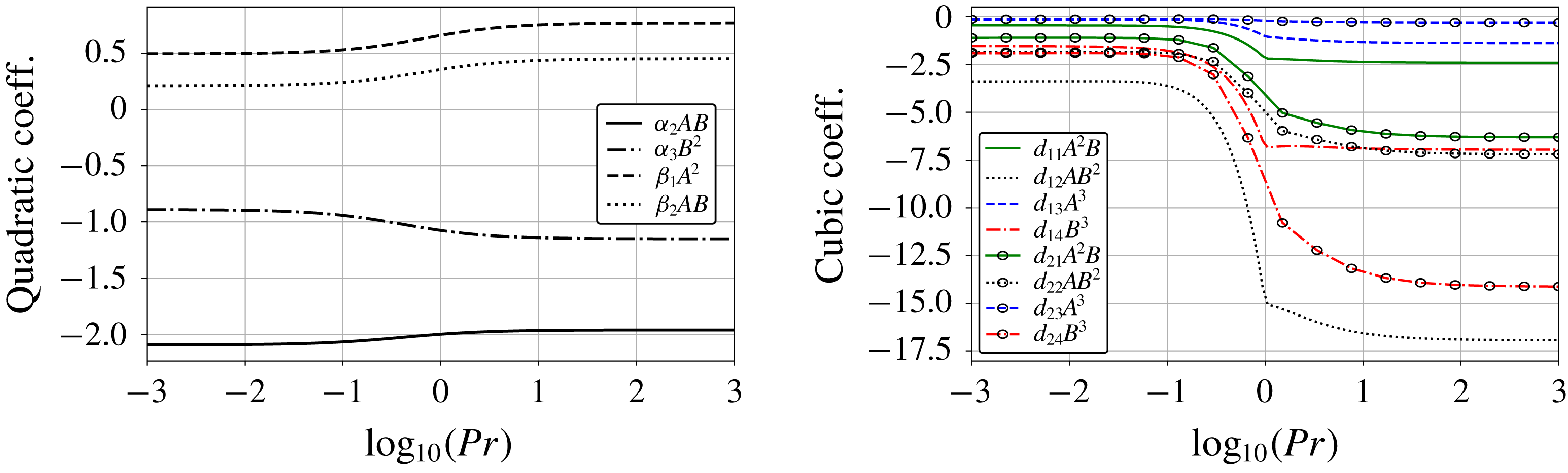
This interaction is governed by the equations
 $$\begin{eqnarray}\left.\begin{array}{@{}c@{}}{\dot{A}}=\unicode[STIX]{x1D707}_{1}A+\unicode[STIX]{x1D6FC}_{2}AB+\unicode[STIX]{x1D6FC}_{3}B^{2}+d_{11}A^{2}B+d_{12}AB^{2}+d_{13}A^{3}+d_{14}B^{3},\\ {\dot{B}}=\unicode[STIX]{x1D707}_{2}B+\unicode[STIX]{x1D6FD}_{1}A^{2}+\unicode[STIX]{x1D6FD}_{2}AB+d_{21}A^{2}B+d_{22}AB^{2}+d_{23}A^{3}+d_{24}B^{3},\end{array}\right\}\begin{array}{@{}l@{}}A\sim \ell \quad \text{even}\\ B\sim \ell \pm 2.\end{array}\end{eqnarray}$$
The quadratic coefficients
 $\unicode[STIX]{x1D6FC}_{i},\unicode[STIX]{x1D6FD}_{i}$
have opposite signs, and the cubic coefficients remain negative as shown in figure 11, so that (5.7) may have mixed mode solutions only. In contrast to the neighbouring mode interactions no pure mode solutions exist, as (5.7) no longer has symmetry.
Bifurcation diagram of the even–even interactions (a)
 $\ell =2,4$
and (b)
 $\ell =4,6$
with
 $Pr=10$
. Region
 $1$
contains two mixed modes
 $(A_{1},+B_{1}),(A_{2},-B_{2})$
; region
 $2$
two stable and unstable mixed modes; region
 $3$
a single stable fixed point; and region 4 two stable spirals
 $(-A_{1},B_{1}),(-A_{2},B_{2})$
. The 3-D stability of axisymmetric solutions at large
 $Pr$
is shown in colour inset (cf. § 7). (a) Within the red hatched region
 $(A,B)$
is stable, but below loses stability to
 $m=2,3$
. (b) Within the densely hatched region (left)
 $(A,B)$
is stable and in the lightly hatched region (right)
 $-(A,B)$
is stable. Below these regions the unstable azimuthal wavenumber
 $m$
varies.

Figure 12 shows the bifurcation diagram and figure 13 the corresponding phase plane for the even–even mode interaction. The absence of symmetry in (5.7) results in two distinct fixed points in each region of 12. In region
 $4$
where the
 $\ell$
mode dominates there are two stable spiral nodes. Transitioning to region
 $3$
via an unstable Hopf bifurcation there is a single stable fixed point. Transitioning into region
 $2$
and subsequently region
 $1$
where the
 $\ell +2$
mode dominates, an additional stable fixed point appears.
Phase-plane diagrams
 $(A,B)$
describing the even–even interaction for mode numbers
 $\ell =2,4$
and
 $Pr=10$
. In region 1 mixed modes
 $(A_{1},+B_{1}),(A_{2},-B_{2})$
exist; in region 2 two stable and unstable mixed modes; in region 3 a single stable mixed mode; while in region 4 two stable spiral nodes
 $(-A_{1},B_{1}),(A_{2},B_{2})$
are obtained.

6 Comparison with direct numerical simulation
Equations (4.29)–(4.33), derived using weakly nonlinear theory, apply rigorously only in an
 $O(\unicode[STIX]{x1D716})$
neighbourhood of the degenerate points
 $(d_{c},Ra_{c})$
seen in figure 4. For this reason it is reasonable to question their validity in the context of the full problem. We validate previous results by performing DNS of the full equations (2.6). The numerical code is spectral in
 $\unicode[STIX]{x1D703}$
and uses a second order finite difference discretisation radially. A second-order Crank–Nicolson Adams–Bashforth scheme is used for time stepping. A minimum resolution of
 $15$
polynomials in
 $\unicode[STIX]{x1D703}$
and
 $40$
grid points in
 $r$
was used in all computations. Specifying values of
 $(d,Ra)$
a full numerical simulation is run, whose mode amplitudes are computed from the inner products
 $$\begin{eqnarray}A_{num}(t)=\frac{\langle \unicode[STIX]{x1D74D}_{num},\unicode[STIX]{x1D74D}_{\ell }\rangle }{\langle \unicode[STIX]{x1D74D}_{\ell },\unicode[STIX]{x1D74D}_{\ell }\rangle },\quad B_{num}(t)=\frac{\langle \unicode[STIX]{x1D74D}_{num},\unicode[STIX]{x1D74D}_{n}\rangle }{\langle \unicode[STIX]{x1D74D}_{n},\unicode[STIX]{x1D74D}_{n}\rangle },\quad \text{where}~\langle f,g\rangle =\int _{r}\int _{\unicode[STIX]{x1D703}}\frac{f\,g}{\sin \unicode[STIX]{x1D703}}\,\text{d}r\,\text{d}\unicode[STIX]{x1D703}.\end{eqnarray}$$
Vectors
 $\unicode[STIX]{x1D74D}_{\ell },\unicode[STIX]{x1D74D}_{n}$
are the eigenfunctions (3.11) evaluated at the grid points of the numerical finite difference solution
 $\unicode[STIX]{x1D74D}_{num}$
. For comparison with weakly nonlinear theory, values for
 $\unicode[STIX]{x1D707},\unicode[STIX]{x1D6FF},\unicode[STIX]{x1D716}$
are specified and the solution determined by solving the relevant amplitude equations. Setting
 $\unicode[STIX]{x1D707}=\pm 1$
we obtain
 $$\begin{eqnarray}\unicode[STIX]{x1D716}=\frac{Ra-Ra_{c}}{Ra_{c}},\quad \unicode[STIX]{x1D6FF}=\frac{d-d_{c}}{\unicode[STIX]{x1D716}}.\end{eqnarray}$$
Simulating (4.29)–(4.33) with these values we obtain a solution
 $(A,B)$
, which is rescaled according to the original expansion (4.3). Amplitudes of the weakly nonlinear theory are obtained as
 $$\begin{eqnarray}A_{wkly}=\unicode[STIX]{x1D716}A,\quad B_{wkly}=\unicode[STIX]{x1D716}B.\end{eqnarray}$$
6.1 Neighbouring mode interactions
Numerical solutions
 $\unicode[STIX]{x1D713}(r,\unicode[STIX]{x1D703})$
in the neighbourhood of the
 $\ell =2,3$
degenerate point (
 $d_{c}=1.9883,Ra_{c}=857.53$
) for
 $Pr=1$
. (a) Corresponds to region
 $3$
of figure 7 for the
 $\ell =2$
mode
 $(d_{c},Ra=900.0)$
, (b) region
 $3$
for the mixed
 $(d=1.946,Ra=950.0)$
, (c) region
 $4$
the mixed
 $(d=1.9481,Ra=900.0)$
.

Comparison of DNS
 $(A,B)_{num}$
and weakly nonlinear
 $(A,B)_{wkly}$
solutions for the modes
 $\ell =2,3$
. The discrepancy between theory and simulation is attributed to the even
 $\ell =4$
mode contribution, found to be non-negligible in DNS, particularly for the mixed solutions in region 3 where both modes are linearly unstable. The odd mode component of mixed solutions maintains a larger amplitude.

The even–odd case is simulated for parameter values corresponding to regions
 $3$
and
 $4$
of figure 7 where both mixed and even solutions are found. This region is chosen in order to test the initial condition dependency predicted by theory. In the initial condition dependent region
 $3$
, even solutions are readily obtained from even initial conditions, as the linear stability of the even solutions tends to ensure that the solution remains even. Mixed solutions are not so easy to find, but can be located by continuation from the mixed solutions of region
 $4$
. The numerical values of each mode shown in table 1 confirm that odd modes maintain a larger amplitude in mixed mode solutions. Corresponding solutions of the flow field are shown in figure 14.
Numerical solutions
 $\unicode[STIX]{x1D713}(r,\unicode[STIX]{x1D703})$
in the neighbourhood of the
 $\ell =3,4$
degenerate point (
 $d_{c}=1.2291,Ra_{c}=2381.1$
) with
 $Pr=1$
. (a) Corresponds to region
 $3$
of figure 9 for the
 $n=4$
mode
 $(d=1.2291,Ra=2650.0)$
, (b) region
 $3$
for the mixed
 $(d=1.2674,Ra_{c})$
, (c) region
 $4$
for the mixed
 $(d=1.2674,Ra=2230.0)$
.

A similar procedure is adopted for the odd–even case to simulate mixed solutions in region
 $3$
of figure 9. Only in certain sections of region
 $3$
are even solutions found to be stable to odd mode perturbations. In addition to finding solutions corresponding to figure 9, the ratio of mixed mode amplitudes also matches well for even solutions in region
 $3$
and mixed solutions in region
 $4$
(see tables 1 and 2). For mixed solutions in region
 $3$
, however, the contribution of modes
 $\ell =2,4$
becomes non-negligible for the values of
 $\unicode[STIX]{x1D716}$
considered. The discrepancy between theory and DNS is attributed to the omission of these modes for the respective cases. Corresponding solutions of the flow field are shown in figure 15.
Comparison of DNS and weakly nonlinear solutions for the modes
 $\ell =3,4$
. The discrepancy between theory and simulation is attributed to the
 $\ell =2$
mode contribution, found to be non-negligible in DNS, particularly for the mixed solutions in region 3 where both modes are linearly unstable. The odd mode component of mixed solutions maintains a larger amplitude.

6.2 Non-neighbouring mode interactions
The even–even interaction described by (4.33) may seem of limited relevance, as solutions obtained for small
 $\unicode[STIX]{x1D716}$
are necessarily unstable to odd mode perturbations. A rigorous reduced-order model of this interaction point would therefore have to include the effect of unstable intermediate modes for example, the
 $\ell =3$
mode in the
 $(\ell =2,4)$
case. However, when we compute the stability of saturated solutions for large
 $\unicode[STIX]{x1D716}$
in § 7, we find that some even solutions are in fact stable to odd perturbations. Such interactions are also thought to exhibit strong resonances and be of physical significance in mantle convection (Chossat & Stewart Reference Chossat, Stewart and Yuen1992). We compare DNS runs with and without screening of the odd modes to determine their validity for the fully nonlinear problem.
Symmetric solutions
 $\unicode[STIX]{x1D713}(r,\unicode[STIX]{x1D703})$
near the
 $\ell =2,4$
degenerate point (
 $d_{c}=1.5807,Ra_{c}=1515.399$
) for
 $Pr=10$
. Panel (a) corresponds to region
 $1$
of figure 12 with
 $(d=1.5507,Ra=1591.392)$
, (b) region
 $3$
for
 $(d_{c},Ra=1591.392)$
, and (c) region
 $4$
for
 $(d=1.6132,Ra=1480)$
. In (a) and (c) only modes
 $\ell =4$
and
 $\ell =2$
respectively are linearly unstable.

Comparison of numerical and weakly nonlinear solutions for the modes
 $\ell =2,4$
. By removing all odd modes the dominance of the remaining modes is increased and an improved agreement between computation and theory is obtained.

Unsurprisingly, the screened simulations (figure 16) near the
 $\ell =2,4$
degenerate point are found to agree better with theory than those with odd modes. The numerical values are outlined in table 3. Given that the solution energy is quantised between fewer linearly unstable modes this improved agreement is anticipated.
For the same parameter values, unscreened simulations near the
 $\ell =2,4$
point lose stability to odd mode perturbations as expected, with significant components of modes
 $\ell =1,2,3,4$
remaining. Increasing the Rayleigh number beyond
 $Ra\approxeq 1.7Ra_{c}$
(measured from the
 $\ell =2,4$
degenerate point), stable mixed periodic solutions emerge for low
 $Pr$
. This is depicted in figure 17 where the amplitude of each mode is plotted as a function of time. Granted that no oscillatory solutions are found for two mode interactions we enquire: Why are odd mode components necessary to maintain a regular oscillation? And why is the oscillation period of even modes approximately twice that of odd modes? We stress that these time-periodic solutions emerge for
 $\unicode[STIX]{x1D716}\sim O(1),Pr\ll 1$
and are, strictly speaking, beyond the scope of weakly nonlinear theory. Nonetheless using the structure of (1.1) it is possible to explain their oscillation signature.
DNS oscillation signature for the periodic solutions near the even–even and odd–odd degeneracies with
 $Pr=0.05$
. Solutions are simulated at (a)
 $Ra_{c}=440.852,\unicode[STIX]{x1D716}=5.85$
, (b)
 $Ra_{c}=1515.41,\unicode[STIX]{x1D716}=0.847$
, (c)
 $Ra_{c}=3425.94,\unicode[STIX]{x1D716}=0.4594$
. Notably the Rayleigh number required to sustain oscillations increases as
 $\ell ,n$
decrease. Even modes oscillate out of phase with equal period, while the odd mode oscillates with double the period of even modes. As the mode numbers increase additional modes contribute and the signal becomes increasingly modulated. Animations corresponding to panels (a), (b), (c) may be found online as Movie 1, Movie 2, Movie 3, respectively at https://doi.org/10.1017/jfm.2019.440.

6.3 Oscillation signature
A distinctive feature of the time-periodic solutions shown in figure 17 is that even and odd modes oscillate with approximately a
 $2:1$
frequency ratio. Also notable is that the time signature for smaller
 $d$
becomes increasingly modulated when compared with that of lower mode numbers. Running DNS near each degeneracy with odd modes suppressed we find that the time periodic solutions presented in figure 17 no longer persist. This suggests the bifurcation to time-periodic solutions at low
 $Pr$
is an odd mode instability.
We attribute the
 $2:1$
resonance to a double-Hopf bifurcation whose weakly nonlinear behaviour may be described locally by a complex analogue of (5.5) cf. (Knobloch & Proctor Reference Knobloch and Proctor1988; Proctor & Jones Reference Proctor and Jones1988). Thus by dictating the nonlinear terms permissible in (5.5) the eigenfunctions constrain the phase of even and odd modes in standing wave solutions. Near the
 $\ell =1,3$
degeneracy, the set of contributing modes is small so that few harmonics are generated. At higher degeneracies, more modes contribute generating additional harmonics which modulate the oscillation signature observed in figure 17.
7 Stability of axisymmetric solutions to azimuthal perturbations
Due to the degeneracy of the linear eigenvalue problem (Busse Reference Busse1975) one cannot determine whether the preferred motion is axisymmetric or non-axisymmetric without considering the nonlinear terms. Given that the analysis of the fully three-dimensional problem is both more complicated and involved, only the axisymmetric problem has so far been investigated in this paper. The validity of solutions presented for the full problem is now investigated by computing their stability to non-axisymmetric perturbations. Following Zebib et al. (Reference Zebib, Schubert and Straus1980, Reference Zebib, Schubert, Dein and Paliwal1983), who numerically investigated the case with stress-free boundary conditions, we simplify the problem by considering the limit
 $Pr\rightarrow \infty$
. In addition to this calculation being simpler, we anticipate that the flow is most likely to remain axisymmetric for large
 $Pr$
, as for low
 $Pr$
advection terms in the momentum equation become destabilising (Jones & Moore Reference Jones and Moore1978).
The equations governing the three-dimensional problem for
 $Pr\rightarrow \infty$
with homogeneous no-slip boundary conditions are
 $$\begin{eqnarray}\left.\begin{array}{@{}c@{}}Ra\unicode[STIX]{x1D735}\times (\boldsymbol{r}g(r)T)+\unicode[STIX]{x1D735}\times \unicode[STIX]{x1D6FB}^{2}\boldsymbol{u}=0,\\ \displaystyle \frac{\unicode[STIX]{x2202}T}{\unicode[STIX]{x2202}t}+\boldsymbol{u}\boldsymbol{\cdot }\unicode[STIX]{x1D735}(T+T_{0}(r))=\unicode[STIX]{x1D6FB}^{2}T,\quad \unicode[STIX]{x1D735}\boldsymbol{\cdot }\boldsymbol{u}=0.\end{array}\right\}\end{eqnarray}$$
The solenoidal velocity field
 $\boldsymbol{u}$
can be expressed in terms of its poloidal and toroidal components
 $$\begin{eqnarray}\boldsymbol{u}=\unicode[STIX]{x1D735}\times \unicode[STIX]{x1D735}\times \left(\frac{\unicode[STIX]{x1D6F7}}{r}\boldsymbol{r}\right)+\unicode[STIX]{x1D735}\times \left(\frac{\unicode[STIX]{x1D6F9}}{r}\boldsymbol{r}\right),\end{eqnarray}$$
which automatically satisfy continuity. In the limit
 $Pr\rightarrow \infty$
, however, the flow may be shown to be purely poloidal,
 $\unicode[STIX]{x1D6F9}\rightarrow 0$
(Zebib et al.
Reference Zebib, Schubert and Straus1980), so that by substituting (7.2) into (7.1) and operating on the momentum equation with
 $\boldsymbol{r}\boldsymbol{\cdot }\unicode[STIX]{x1D735}\times$
, one can express (7.1) in terms of
 $\unicode[STIX]{x1D6F7}$
and
 $T$
only. This allows the problem to be recast as
 $$\begin{eqnarray}\left(\begin{array}{@{}cc@{}}0 & 0\\ 0 & 1\end{array}\right)\left(\begin{array}{@{}c@{}}\unicode[STIX]{x1D6F7}_{t}\\ T_{t}\end{array}\right)=\left(\begin{array}{@{}cc@{}}\unicode[STIX]{x1D6FB}^{2}\unicode[STIX]{x1D6FB}^{2}(r^{-1}) & -Ra\,g(r)\\ -(T_{0}^{\prime }(r)/r^{2})L^{2} & \unicode[STIX]{x1D6FB}^{2}\end{array}\right)\left(\begin{array}{@{}c@{}}\unicode[STIX]{x1D6F7}\\ T\end{array}\right)-\left(\begin{array}{@{}c@{}}0\\ \boldsymbol{u}\boldsymbol{\cdot }\unicode[STIX]{x1D735}T\end{array}\right),\end{eqnarray}$$
where the velocity vector
 $\boldsymbol{u}$
and the operator
 $L^{2}$
are given by
 $$\begin{eqnarray}\boldsymbol{u}=\left(\frac{L^{2}\unicode[STIX]{x1D6F7}}{r^{2}},\frac{1}{r}\frac{\unicode[STIX]{x2202}^{2}\unicode[STIX]{x1D6F7}}{\unicode[STIX]{x2202}r\unicode[STIX]{x2202}\unicode[STIX]{x1D711}},\frac{1}{r\sin \unicode[STIX]{x1D703}}\frac{\unicode[STIX]{x2202}^{2}\unicode[STIX]{x1D6F7}}{\unicode[STIX]{x2202}r\unicode[STIX]{x2202}\unicode[STIX]{x1D711}}\right),\quad L^{2}\equiv -\frac{1}{\sin \unicode[STIX]{x1D703}}\frac{\unicode[STIX]{x2202}}{\unicode[STIX]{x2202}\unicode[STIX]{x1D703}}\sin \unicode[STIX]{x1D703}\frac{\unicode[STIX]{x2202}}{\unicode[STIX]{x2202}\unicode[STIX]{x1D703}}-\frac{1}{\sin ^{2}\unicode[STIX]{x1D703}}\frac{\unicode[STIX]{x2202}^{2}}{\unicode[STIX]{x2202}\unicode[STIX]{x1D711}^{2}}.\end{eqnarray}$$
The scalar
 $\unicode[STIX]{x1D6F7}$
is related to the Stokes streamfunction by
 $\unicode[STIX]{x1D713}=-\text{sin}\,\unicode[STIX]{x1D703}(\unicode[STIX]{x2202}\unicode[STIX]{x1D6F7}/\unicode[STIX]{x2202}\unicode[STIX]{x1D703})$
. To compute the stability of an axisymmetric steady state
 $(\unicode[STIX]{x1D6F7},T)^{\text{T}}$
we add a non-axisymmetric perturbation
 $(\unicode[STIX]{x1D716}\unicode[STIX]{x1D6F7}^{\prime },\unicode[STIX]{x1D716}T^{\prime })^{\text{T}}$
and retaining terms of
 $O(\unicode[STIX]{x1D716})$
obtain the linear system
 $$\begin{eqnarray}\unicode[STIX]{x1D706}{\mathcal{M}}\boldsymbol{X}^{\prime }={\mathcal{L}}\boldsymbol{X}^{\prime }-\left(\begin{array}{@{}cc@{}}0 & 0\\ N_{1}(T) & N_{2}(\unicode[STIX]{x1D6F7})\end{array}\right)\boldsymbol{X}^{\prime },\quad \text{where}~\boldsymbol{X}^{\prime }=(\unicode[STIX]{x1D6F7}^{\prime },T^{\prime })^{\text{T}}.\end{eqnarray}$$
The matrix operators
 ${\mathcal{M}},{\mathcal{L}}$
are those of (7.3) and the terms
 $N_{1}(T)$
and
 $N_{2}(\unicode[STIX]{x1D6F7})$
come from the linearisation of
 $\boldsymbol{u}\boldsymbol{\cdot }\unicode[STIX]{x1D735}T$
. In writing (7.5) we have assumed that
 $\boldsymbol{X}^{\prime }$
has exponential time dependency. To compute the growth rate
 $\unicode[STIX]{x1D706}\in \mathbb{R}$
we represent the numerically determined axisymmetric state by a finite sum of Legendre polynomials
 $$\begin{eqnarray}\unicode[STIX]{x1D6F7}\simeq \mathop{\sum }_{p=1}^{N_{\unicode[STIX]{x1D703}}}\unicode[STIX]{x1D6F7}_{p}(r)P_{p}(\cos \unicode[STIX]{x1D703}),\quad T\simeq \mathop{\sum }_{p=0}^{N_{\unicode[STIX]{x1D703}}}T_{p}(r)P_{p}(\cos \unicode[STIX]{x1D703}),\end{eqnarray}$$
and the perturbation by a finite sum of associated Legendre polynomials
 $$\begin{eqnarray}\unicode[STIX]{x1D6F7}^{\prime }\simeq \mathop{\sum }_{\ell =m}^{N_{\unicode[STIX]{x1D703}}}\unicode[STIX]{x1D6F7}_{\ell m}^{\prime }(r)P_{\ell }^{m}(\cos \unicode[STIX]{x1D703})\text{e}^{\text{i}m\unicode[STIX]{x1D711}},\quad T^{\prime }\simeq \mathop{\sum }_{\ell =m}^{N_{\unicode[STIX]{x1D703}}}T_{\ell m}^{\prime }(r)P_{\ell }^{m}(\cos \unicode[STIX]{x1D703})\text{e}^{\text{i}m\unicode[STIX]{x1D711}}.\end{eqnarray}$$
Representation in this manner allows the
 $\unicode[STIX]{x1D703}$
-dependency of (7.5) to be integrated out, yielding a system of
 $N_{\unicode[STIX]{x1D703}}$
coupled ODEs dependent on the radial coordinate
 $r$
and azimuthal wavenumber
 $m$
only. Discretising the radial direction using second-order finite differences, the growth rate
 $\unicode[STIX]{x1D706}$
is computed for a range of
 $Ra$
and different
 $m$
. The results of this computation are summarised in tables 4 and 5 and have been included as neutral stability curves
 $\unicode[STIX]{x1D706}(\unicode[STIX]{x1D6FF},\unicode[STIX]{x1D707},m)=0$
in the bifurcations diagrams presented in § 5 figures 6, 9 and 12. For ease of comparison with these figures the parameters
 $$\begin{eqnarray}\unicode[STIX]{x1D707}=(Ra-Ra_{c})/Ra_{c},\quad \unicode[STIX]{x1D6FF}=d-d_{c}\end{eqnarray}$$
are used. As before,
 $(d_{c},Ra_{c})$
represents the coordinates of a given degenerate point.
Three-dimensional stability at large
 $Pr$
and
 $\unicode[STIX]{x1D6FF}=0$
of axisymmetric solutions to azimuthal perturbations of wavenumber
 $m$
at each
 $(\ell ,\ell +1)$
degeneracy. In all cases the
 $Ra$
required for 3-D stability is measured from the degenerate point
 $(d_{c},Ra_{c})$
specific to each case. The stability of solutions is denoted
 $U=\text{unstable for }\unicode[STIX]{x1D706}>0$
,
 $S=\text{stable for }\unicode[STIX]{x1D706}<0$
or
 $N=\text{neutral}$
in the special case where the
 $m=1$
mode is neutrally stable. Higher wavenumbers
 $m>4$
were found to be stable for the range of
 $Ra$
considered.

Three-dimensional stability at large
 $Pr$
and
 $\unicode[STIX]{x1D6FF}=0$
of axisymmetric solutions at even
 $(\ell ,\ell +2)$
degeneracies to azimuthal perturbations of wavenumber
 $m$
. Higher wavenumbers
 $m>4$
were found to be stable for the range of
 $Ra$
considered.

The results are broadly similar to those of Zebib et al. (Reference Zebib, Schubert and Straus1980, Reference Zebib, Schubert, Dein and Paliwal1983) who considered the case of stress-free boundaries. In general our calculations indicate that just above the critical
 $Ra_{c}$
axisymmetric solutions are unstable to some azimuthal wavenumbers, but once established at larger
 $Ra$
we find that solutions stabilise. Therefore in this regime the axisymmetric flows are stable solutions of the full 3-D system (7.1), although they need not be the preferred state for arbitrary initial conditions. Because of the reflectional symmetry of mixed solutions, it is only necessary to consider three solution types in tables 4 and 5. An azimuthal wavenumber
 $m$
is denoted by
 $U$
for unstable if
 $\unicode[STIX]{x1D706}>0$
, S for stable if
 $\unicode[STIX]{x1D706}<0$
and
 $N$
for neutrally stable if
 $\unicode[STIX]{x1D706}=0$
.
7.1 Odd–even and even–odd interactions
The stability of solutions for different
 $(\unicode[STIX]{x1D6FF},\unicode[STIX]{x1D707})$
is computed and the region of parameter space for which the axisymmetric solutions are stable is included in figures 6 and 9. Specifically we find that near the
 $\ell =(1,2)$
degenerate point, even solutions
 $(0,\pm B)$
are stable in regions 3 and 6 of figure 9, while mixed solutions
 $(\pm A,B)$
are stable in region 4 only. Near the
 $\ell =(2,3)$
degenerate point, even solutions
 $(-A,0)$
are stable only for large
 $\unicode[STIX]{x1D6FF},\unicode[STIX]{x1D707}$
, as shown in figure 6. Stable mixed solutions are found for
 $\unicode[STIX]{x1D6FF}<0.22$
, but above this threshold are destabilised by
 $m=2$
. Near the
 $\ell =(3,4)$
degenerate point, stable solutions of both even and mixed form are found. For
 $\unicode[STIX]{x1D6FF}>0$
the mixed solutions are stable, while for
 $\unicode[STIX]{x1D6FF}<0.2$
stable even mode solutions are found as shown in figure 9. Notably, the stability behaviour of different even solutions near the same degeneracy can vary. It was shown by Zebib et al. (Reference Zebib, Schubert and Straus1980, Reference Zebib, Schubert, Dein and Paliwal1983) for the case of stress-free boundaries, that the heat transfer achieved by each of these solutions differs as
 $\unicode[STIX]{x1D707}$
is increased from the bifurcation point. Our numerical simulations identify similar behaviour for the even mode cases. Results for
 $\unicode[STIX]{x1D6FF}=0$
are summarised in table 4 to indicate the behaviour of different azimuthal wavenumbers.
7.2 Even–even interactions
Despite the presence of linearly unstable odd modes near even–even degeneracies, stable even solutions of the full problem may also be found. Near the
 $\ell =(2,4)$
degeneracy solutions are stable to axisymmetric odd mode perturbations for
 $\unicode[STIX]{x1D707}>0.87$
and to all non-axisymmetric perturbations for
 $\unicode[STIX]{x1D707}>1.01$
. These thresholds are however larger than those of neighbouring
 $\ell ,\ell \pm 1$
degeneracies. Near the
 $\ell =(4,6)$
degeneracy solutions are found to be stable above a threshold whose unstable wavenumber
 $m$
varies with
 $\unicode[STIX]{x1D6FF}$
as shown in figure 12. Notably, the threshold for 3-D stability at the
 $\ell =(4,6)$
degeneracy is lower than that of the
 $\ell =(2,4)$
case. Results for
 $\unicode[STIX]{x1D6FF}=0$
are summarised in table 5 to indicate the behaviour of different azimuthal wavenumbers.
8 Discussion
Equations (4.29)–(4.33) are derived using weakly nonlinear theory and apply, strictly, only within a small region of the degenerate points. Nevertheless, using DNS and 3-D stability calculations we have demonstrated their extended value, in particular the insight they provide into the form of the dominant nonlinearities and the role of
 $Pr$
. The latter is a numerically challenging task granted the large diffusion times for both small and large
 $Pr$
. The physical implications of these equations are now considered.
The spatial resonances between odd and even modes are found to be central in the description of spherical convection. Contributing quadratic terms to the amplitude equations they limit both the range of possible fixed points and the relative frequencies of odd and even modes in periodic solutions. Only even modes can have pure mode solutions, while odd modes can exist only as the larger component of mixed mode solutions. Mapping out the parameter space near degenerate points it is found that stable solutions may be initial condition dependent, and that hysteresis exists between pure and mixed mode states. This behaviour has also been reported by Kidachi (Reference Kidachi1982) and Knobloch & Guckenheimer (Reference Knobloch and Guckenheimer1983) for planar geometries. While these results are easily verified using full numerical simulation, the range of possible solutions and their stability is not readily apparent without the aid of amplitude equations.
A surprising result is the presence of standing wave solutions for
 $Pr\ll 1$
in which the even and odd components of solutions oscillate in a
 $2:1$
frequency ratio. Notably, this relation appears general to all standing wave solutions and persists for large
 $Ra$
provided
 $d\geqslant 1$
. While these solutions are likely to become unstable to non-axisymmetric perturbations, we suspect that this relation will hold for standing wave solutions in a fully 3-D spherical annulus. This is on the basis that equations derived by Friedrich & Haken (Reference Friedrich and Haken1986) and Beltrame & Chossat (Reference Beltrame and Chossat2015) to describe the
 $(1,2)$
and
 $(3,4)$
mode interactions in a fully 3-D domain possess a structure identical to (5.1).
Investigating the stability of axisymmetric states calculated for three-dimensional perturbations, we found that slightly above the onset of convection, axisymmetric solutions are stable solutions of the full problem for large
 $Pr$
. In particular, even axisymmetric solutions near even–even degeneracies, despite being linearly unstable at onset, are found to stabilise. It is possible that for arbitrary initial conditions, a large amplitude non-axisymmetric state might be preferred.
While the approach adopted in this paper has used significant simplifications, it appears a useful reduction, as it predicts the amplitude of the flow using just two coupled ODEs. Compared to the large dimension of systems obtained when studying the 3-D problem either numerically, or by analogous model reduction methods, this is a vast simplification. We would finally like to emphasise that while the results presented focus on small
 $(\ell ,n)$
, the theory derived applies generally to any combination of two degenerate modes. We anticipate the greatest relevance for wide spherical shells,
 $d>1$
, as the degenerate points are widely spaced for the small mode numbers typical of that regime.
Supplementary movies
Supplementary movies are available at https://doi.org/10.1017/jfm.2019.440.
Appendix A. Self-adjointness of the operator
${\mathcal{L}}$

For a vector
 $\unicode[STIX]{x1D753}$
and operator
 ${\mathcal{L}}$
as outlined
 $$\begin{eqnarray}\unicode[STIX]{x1D753}=\left(\begin{array}{@{}c@{}}\unicode[STIX]{x1D713}(r,\unicode[STIX]{x1D703})\\ T(r,\unicode[STIX]{x1D703})\end{array}\right),\quad {\mathcal{L}}=\left(\begin{array}{@{}cc@{}}D^{2}D^{2} & Ra_{c}g(r)\sin \unicode[STIX]{x1D703}\displaystyle \frac{\unicode[STIX]{x2202}}{\unicode[STIX]{x2202}\unicode[STIX]{x1D703}}\\ -\displaystyle \frac{T_{0}^{\prime }}{r}\frac{1}{\sin \unicode[STIX]{x1D703}}\frac{\unicode[STIX]{x2202}}{\unicode[STIX]{x2202}\unicode[STIX]{x1D703}} & \hat{D}^{2}\end{array}\right),\end{eqnarray}$$
an inner product may be found such that
 $$\begin{eqnarray}\langle \unicode[STIX]{x1D753}^{+},{\mathcal{L}}\unicode[STIX]{x1D753}\rangle =\langle {\mathcal{L}}\unicode[STIX]{x1D753}^{+},\unicode[STIX]{x1D753}\rangle .\end{eqnarray}$$
Operators
 $D^{2}$
and
 $\hat{D}^{2}$
are defined as
 $$\begin{eqnarray}D^{2}=\frac{\unicode[STIX]{x2202}^{2}}{\unicode[STIX]{x2202}r^{2}}+\frac{\sin \unicode[STIX]{x1D703}}{r^{2}}\frac{\unicode[STIX]{x2202}}{\unicode[STIX]{x2202}\unicode[STIX]{x1D703}}\left(\frac{1}{\sin \unicode[STIX]{x1D703}}\frac{\unicode[STIX]{x2202}}{\unicode[STIX]{x2202}\unicode[STIX]{x1D703}}\right),\quad \hat{D}^{2}=\frac{\unicode[STIX]{x2202}^{2}}{\unicode[STIX]{x2202}r^{2}}+\frac{1}{r^{2}\sin \unicode[STIX]{x1D703}}\frac{\unicode[STIX]{x2202}}{\unicode[STIX]{x2202}\unicode[STIX]{x1D703}}\left(\sin \unicode[STIX]{x1D703}\frac{\unicode[STIX]{x2202}}{\unicode[STIX]{x2202}\unicode[STIX]{x1D703}}\right).\end{eqnarray}$$
Assuming homogeneous boundary conditions (2.9) a sufficient condition for this system to be self-adjoint requires that the functional form of the temperature gradient and gravity field
 $g(r)$
satisfy
 $$\begin{eqnarray}\frac{\text{d}}{\text{d}r}\frac{g(r)r}{T_{0}^{\prime }}=0.\end{eqnarray}$$
The relevant inner product or volume integral is defined as
 $$\begin{eqnarray}\left\langle \left(\begin{array}{@{}c@{}}\displaystyle \frac{A_{T}\unicode[STIX]{x1D713}^{+}(r,\unicode[STIX]{x1D703})}{Ra_{c}r^{2}\sin ^{2}\unicode[STIX]{x1D703}}\\ \displaystyle \frac{T^{+}(r,\unicode[STIX]{x1D703})}{r^{2}}\end{array}\right),\left(\begin{array}{@{}cc@{}}D^{2}D^{2} & Ra_{c}g(r)\sin \unicode[STIX]{x1D703}\displaystyle \frac{\unicode[STIX]{x2202}}{\unicode[STIX]{x2202}\unicode[STIX]{x1D703}}\\ -\displaystyle \frac{T_{0}^{\prime }}{r}\frac{1}{\sin \unicode[STIX]{x1D703}}\frac{\unicode[STIX]{x2202}}{\unicode[STIX]{x2202}\unicode[STIX]{x1D703}} & \hat{D}^{2}\end{array}\right)\left(\begin{array}{@{}c@{}}\unicode[STIX]{x1D713}(r,\unicode[STIX]{x1D703})\\ T(r,\unicode[STIX]{x1D703})\end{array}\right)\right\rangle =\langle \unicode[STIX]{x1D753}^{+},{\mathcal{L}}\unicode[STIX]{x1D753}\rangle ,\end{eqnarray}$$
where the additional factors included are chosen to satisfy (A 2). Provided
 $T_{0}^{\prime }/r=A_{T}g(r)$
this can be expanded as a volume integral with
 $g(r)$
factorised so that one obtains
 $$\begin{eqnarray}\displaystyle & & \displaystyle \int _{\unicode[STIX]{x1D703}}\int _{r}\left\{\frac{A_{T}\unicode[STIX]{x1D713}^{+}}{Ra_{c}r^{2}\sin ^{2}\unicode[STIX]{x1D703}}D^{2}D^{2}\unicode[STIX]{x1D713}+\frac{A_{T}g(r)}{r^{2}}\left(\unicode[STIX]{x1D713}^{+}\frac{1}{\sin \unicode[STIX]{x1D703}}\frac{\unicode[STIX]{x2202}T}{\unicode[STIX]{x2202}\unicode[STIX]{x1D703}}-T^{+}\frac{1}{\sin \unicode[STIX]{x1D703}}\frac{\unicode[STIX]{x2202}\unicode[STIX]{x1D713}}{\unicode[STIX]{x2202}\unicode[STIX]{x1D703}}\right)\right.\nonumber\\ \displaystyle & & \displaystyle \quad +\left.\frac{T^{+}}{r^{2}}\hat{D}^{2}T\right\}r^{2}\sin \unicode[STIX]{x1D703}\,\text{d}r\,\text{d}\unicode[STIX]{x1D703}.\end{eqnarray}$$
As the Stokes operator
 $D^{2}$
and the operator
 $\hat{D}^{2}$
may be related to the Laplacian (which for homogeneous boundary conditions is self-adjoint) using
 $$\begin{eqnarray}\frac{1}{r\sin \unicode[STIX]{x1D703}}D^{2}\unicode[STIX]{x1D713}=\left(\unicode[STIX]{x1D6FB}^{2}-\frac{1}{r^{2}\sin ^{2}\unicode[STIX]{x1D703}}\right)\frac{\unicode[STIX]{x1D713}}{r\sin \unicode[STIX]{x1D703}},\quad \frac{1}{r}\hat{D}^{2}T=\unicode[STIX]{x1D6FB}^{2}\frac{T}{r},\end{eqnarray}$$
the first and fourth term of (A 6) automatically satisfy (A 2). Considering the second and third terms, we multiply through by factors
 $r^{2}\sin ^{2}\unicode[STIX]{x1D703}$
to yield
 $$\begin{eqnarray}\int _{r}\int _{\unicode[STIX]{x1D703}}A_{T}g(r)\left(\unicode[STIX]{x1D713}^{+}\frac{\unicode[STIX]{x2202}T}{\unicode[STIX]{x2202}\unicode[STIX]{x1D703}}-T^{+}\frac{\unicode[STIX]{x2202}\unicode[STIX]{x1D713}}{\unicode[STIX]{x2202}\unicode[STIX]{x1D703}}\right)\text{d}r\,\text{d}\unicode[STIX]{x1D703}.\end{eqnarray}$$
Integrating by parts with respect to
 $\unicode[STIX]{x1D703}$
we obtain
 $$\begin{eqnarray}\int _{r}A_{T}g(r)\left\{\unicode[STIX]{x1D713}^{+}T|_{\unicode[STIX]{x1D703}=0,\unicode[STIX]{x1D70B}}-\int _{\unicode[STIX]{x1D703}}T\frac{\unicode[STIX]{x2202}\unicode[STIX]{x1D713}^{+}}{\unicode[STIX]{x2202}\unicode[STIX]{x1D703}}\,\text{d}\unicode[STIX]{x1D703}-T^{+}\unicode[STIX]{x1D713}|_{\unicode[STIX]{x1D703}=0,\unicode[STIX]{x1D70B}}+\int _{\unicode[STIX]{x1D703}}\frac{\unicode[STIX]{x2202}T^{+}}{\unicode[STIX]{x2202}\unicode[STIX]{x1D703}}\unicode[STIX]{x1D713}\,\text{d}\unicode[STIX]{x1D703}\right\}\text{d}r.\end{eqnarray}$$
Applying the boundary conditions at
 $\unicode[STIX]{x1D703}=0,\unicode[STIX]{x1D70B}$
terms outside the integral vanish yielding the desired result. Factorising
 $r^{2}\sin \unicode[STIX]{x1D703}$
terms from this expression we may rewrite the expression as
 $$\begin{eqnarray}\int _{r}\int _{\unicode[STIX]{x1D703}}\frac{A_{T}g(r)}{r^{2}}\left\{-\frac{T}{\sin \unicode[STIX]{x1D703}}\frac{\unicode[STIX]{x2202}\unicode[STIX]{x1D713}^{+}}{\unicode[STIX]{x2202}\unicode[STIX]{x1D703}}+\frac{1}{\sin \unicode[STIX]{x1D703}}\frac{\unicode[STIX]{x2202}T^{+}}{\unicode[STIX]{x2202}\unicode[STIX]{x1D703}}\unicode[STIX]{x1D713}\right\}r^{2}\sin \unicode[STIX]{x1D703}\,\text{d}r\,\text{d}\unicode[STIX]{x1D703},\end{eqnarray}$$
so that these terms also satisfy (A 2).



