2 The model

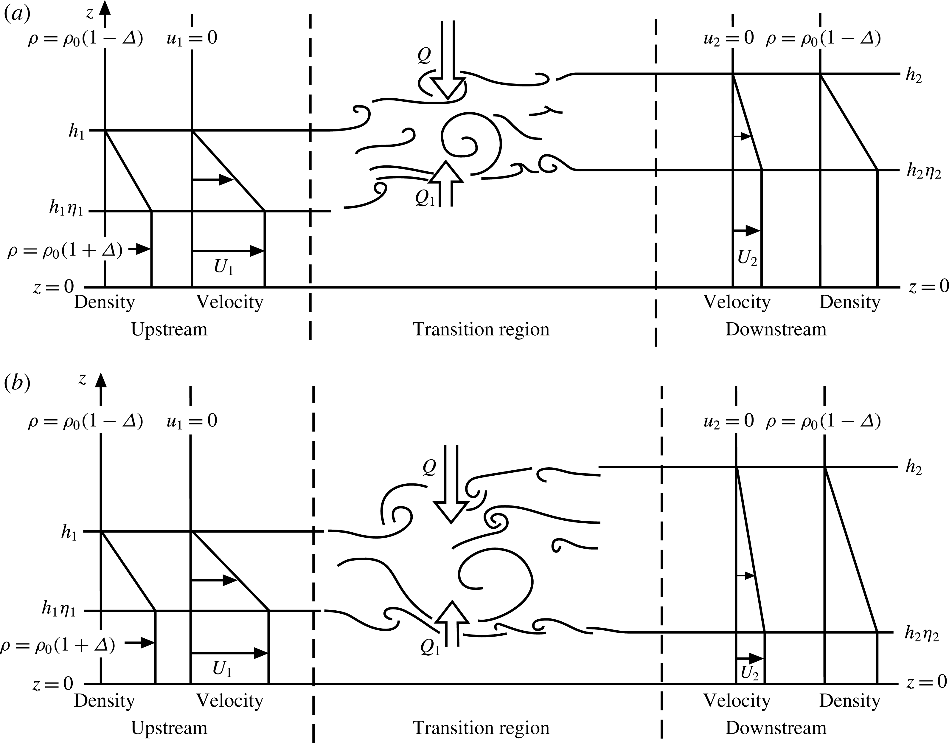
A theoretical model of a stationary turbulent internal hydraulic jump in a non-rotating system was devised by Thorpe & Li (Reference Thorpe and Li2014, hereafter TL) and is illustrated in figure 1. A stratified layer in which the jump occurs flows over a rigid horizontal boundary at $z=0$ and beneath a uniform stationary fluid of infinite depth. Unlike the majority of models of such jumps, which assume that the flow consists of two discrete uniform layers upstream of the hydraulic transition (reviewed, for example, by Baines (Reference Baines2016) and Ogden & Helfich (Reference Ogden and Helfich2016)), TL adopt continuous profiles of velocity and density both upstream and downstream of the transition. The velocities in the model are given by

(2.1) $$\begin{eqnarray}u_{i}(z)=U_{i}F_{i}(z/h_{i}),\end{eqnarray}$$

where $i=1$ indicates a steady flow approaching a jump (‘upstream’) and $i=2$ indicates a steady flow beyond the jump (‘downstream’) when turbulence generated within the region of the transition has collapsed, and $h_{i}$ is the thickness of the flowing layers. The (positive) functions $F_{i}$ are selected as ‘ $\unicode[STIX]{x1D702}$ profiles’; for a given value $\unicode[STIX]{x1D702}_{i}$ and with $y=z/h_{i}$ ,

(2.2) $$\begin{eqnarray}F_{i}(y)=\left\{\begin{array}{@{}ll@{}}1,\quad & \text{if }0\leqslant y\leqslant \unicode[STIX]{x1D702}_{i}\leqslant 1\text{ (a uniform lower layer)},\\ (1-y)/(1-\unicode[STIX]{x1D702}_{i}),\quad & \text{if }\unicode[STIX]{x1D702}_{i}\leqslant y\leqslant 1\text{ (an interfacial layer)},\\ 0,\quad & \text{if }y\geqslant 1\text{ (a uniform and stationary upper layer)}.\end{array}\right.\end{eqnarray}$$

The $\unicode[STIX]{x1D702}$ profiles provide examples of flows ranging from a uniform gradient extending from $z=0$ to $z=h_{i}$ when $\unicode[STIX]{x1D702}_{i}=0$ to a two-layer structure with discontinuity at $z=h_{i}$ when $\unicode[STIX]{x1D702}_{i}=1$ .

Figure 1.

Sketches showing the model representation of a turbulent hydraulic jump or transition in a stratified shear flow over a plane boundary at $z=0$ : (a) a mode 1 transition and (b) a transition of mode 2. Here $Q$ and $Q_{1}$ represent the fluxes of volume of density $\unicode[STIX]{x1D70C}_{0}(1-\unicode[STIX]{x1D6E5})$ from above and of density $\unicode[STIX]{x1D70C}_{0}(1+\unicode[STIX]{x1D6E5})$ from below into the transition zone. (From Thorpe & Li (Reference Thorpe and Li2014); their figure 1.)

The density is chosen with a profile similar to the velocity:

(2.3) $$\begin{eqnarray}\unicode[STIX]{x1D70C}_{i}(z)=\unicode[STIX]{x1D70C}_{0}[1-\unicode[STIX]{x1D6E5}+2\unicode[STIX]{x1D6E5}F_{i}(z/h_{i})].\end{eqnarray}$$

The reference density, $\unicode[STIX]{x1D70C}_{0}$ , and the measure of density variation, $\unicode[STIX]{x1D6E5}$ (and the velocity measures, $U_{i}$ ), are all positive. The density at the boundary, $z=0$ , is $\unicode[STIX]{x1D70C}_{0}(1+\unicode[STIX]{x1D6E5})$ in the upstream flow and also in the downstream flow. (This requirement of equal densities at $z=0$ can be relaxed to allow mixing in the transition to extend through the lower layer down to the seabed, so reducing the density in the downstream flow at $z=0$ and introducing a measure, $\unicode[STIX]{x1D6FF}$ , of the density change, as described by Thorpe (Reference Thorpe2010) and TL.) The density gradients, $\text{d}\unicode[STIX]{x1D70C}_{i}/\text{d}z$ , are zero except in the interfacial layer, where they equal $-2\unicode[STIX]{x1D6E5}\unicode[STIX]{x1D70C}_{0}/[h_{i}(1-\unicode[STIX]{x1D702}_{i})]$ . Above $z=h_{i}$ the density is equal to $\unicode[STIX]{x1D70C}_{0}(1-\unicode[STIX]{x1D6E5})$ and, since the density is uniform, no internal waves can propagate upwards from the transition region (but see appendix C). It is assumed that the transition is not undular; no allowance is made for mixing and energy loss in a train of stationary waves downstream of a jump. The downstream profiles defined by $U_{2}$ , $h_{2}$ and $\unicode[STIX]{x1D702}_{2}$ depend on the turbulent mixing in the jump but are made to be consistent with their upstream values, $U_{1}$ , $h_{1}$ and $\unicode[STIX]{x1D702}_{1}$ , according to the laws of conservation of volume, mass and momentum fluxes.

The $\unicode[STIX]{x1D702}$ profiles at locations upstream and downstream of perceived hydraulic jumps are fitted to the data as explained in appendix A to obtain values of $\unicode[STIX]{x1D702}_{i}$ , $U_{i}$ , $h_{i}$ and $2\unicode[STIX]{x1D6E5}\unicode[STIX]{x1D70C}_{0}$ . The gradient Richardson number in the interfacial layer $(\unicode[STIX]{x1D702}_{i}h_{i}<z<h_{i})$ is

(2.4) $$\begin{eqnarray}\mathit{Ri}_{i}=2g\unicode[STIX]{x1D6E5}h_{i}(1-\unicode[STIX]{x1D702}_{i})/U_{i}^{2}.\end{eqnarray}$$

Closure is obtained by assuming that the downstream interfacial Richardson number, $\mathit{Ri}_{2}$ , equals $1/3$ . This value is chosen because by the Miles–Howard theorem it ensures that the downstream flow is stable. Furthermore, it is well within the bounds of uncertainty of the final values, $\mathit{Ri}_{F}$ , of Richardson numbers in laboratory and numerical studies of decaying turbulence following Kelvin–Helmholtz instability (KHI) in a stratified interfacial layer (e.g. Thorpe Reference Thorpe1973; Smyth, Moum & Caldwell Reference Smyth, Moum and Caldwell2001). It should, however, be noted that whether there is a similar limiting Richardson number following the collapse of turbulence initiated in a hydraulic jump is not known, although a value of approximately $1/3$ is indeed found downstream of the jumps analysed in § 3. The upstream flow is characterized by $\unicode[STIX]{x1D702}_{1}$ and a Froude number, Fr, defined as

(2.5) $$\begin{eqnarray}\mathit{Fr}=U_{1}^{2}/(g\unicode[STIX]{x1D6E5}h_{1})=2(1-\unicode[STIX]{x1D702}_{1})/\mathit{Ri}_{1}.\end{eqnarray}$$

Figure 2 summarizes the analysis of three factors important in internal hydraulic jumps: wave propagation, consistency with the conservation laws, and the stability of the upstream and downstream flows. It shows the character of flows satisfying the conservation laws and the possibility of transitions at points in the ( $\unicode[STIX]{x1D702}_{1},Fr$ ) plane defining the upstream flow. A necessary condition for a steady stationary jump is that no waves can propagate upstream to alter the flow in which the jump occurs. The bold lines of figure 2(a,b) are derived by Thorpe (Reference Thorpe2010, see his § 4.2) and indicate limiting values for this condition to apply. They mark the maximum value of Fr for given $\unicode[STIX]{x1D702}_{1}$ at which waves can propagate in the upstream direction; at greater values of Fr (when jumps can be stationary) there are no upstream-travelling waves. When $\unicode[STIX]{x1D702}_{1}<2/3$ , the limiting Froude number equals $8(1-\unicode[STIX]{x1D702}_{1})$ and (2.5) implies that $\mathit{Ri}_{1}=1/4$ . (The condition $\mathit{Ri}_{1}=1/4$ is satisfied on the dashed line and on its continuation to $\mathit{Fr}=8$ at $\unicode[STIX]{x1D702}_{1}=0$ in figure 2 a,b.) Figure 2(b), found following TL, also shows where finite-amplitude jumps consistent with the conservation laws may be possible in given upstream flows, i.e. at points in the ( $\unicode[STIX]{x1D702}_{1},Fr$ ) plane. To the right of the bold line marking the limiting Fr, the plane is divided into three regions, A, B and C. No jumps are possible in region A. Just one solution of the conservation equations for a flow downstream of a jump is possible in region C (meaning that only one type of jump or mode of transition can occur). Two solutions exist in region B; one of two jumps are possible but only when $\unicode[STIX]{x1D702}_{1}$ exceeds 0.74 and Fr is sufficiently large. Jumps occur in the regions B and C where the upstream flow with corresponding $\unicode[STIX]{x1D702}_{1}$ and Fr is described as ‘supercritical’ to the formation of hydraulic jumps. Jumps are not supported in the remaining regions of the ( $Fr,\unicode[STIX]{x1D702}_{1}$ ) plane; these flows are ‘subcritical’. The smallest Fr at which a jump can occur is 2.2 when $\unicode[STIX]{x1D702}_{1}=0.74$ , at the junction of regions B and C and the bold line. The single roots in region C generally correspond to mode 2 jumps (figure 1 b) in which the interfacial layer in the upstream flow, $\unicode[STIX]{x1D702}_{1}h_{1}<z<h_{1}$ , expands both upwards and downwards; values of $h_{2}$ exceed $h_{1}$ but $\unicode[STIX]{x1D702}_{1}h_{1}>\unicode[STIX]{x1D702}_{2}h_{2}$ , so that the upper isopycnals rise and the lower descend. The double roots of region B are either of mode 2 jumps or those of mode 1, in which all isopycnals rise through the transition as illustrated in figure 1(a).

Figure 2.

A summary of the stability of a flow and hydraulic jumps in the ( $\unicode[STIX]{x1D702}_{1},Fr$ ) plane. (a) Internal waves can propagate upstream in the hatched region, and consequently no stationary hydraulic jumps are formed here. One has $\mathit{Ri}=1/4$ on the line joining ( $\unicode[STIX]{x1D702}_{1}=0$ ,  $Fr=8$ ) to ( $\unicode[STIX]{x1D702}_{1}=1$ ,  $Fr=0$ ), with smaller values of Ri to its right. (b) The region $\mathit{Ri}<1/4$ is divided as follows: A, in which no jumps may occur; B, in which jumps of modes 1 and 2 are possible; and C, in which only one jump, generally of mode 2, is possible. Flows in B and C are supercritical and the remaining area of the ( $\unicode[STIX]{x1D702}_{1},Fr$ ) plane is subcritical. In D, $\mathit{Ri}<1/4$ and the flow is unstable to KHI but, because waves can propagate upstream (as shown in panel (a)), no stationary jumps can occur. (c) The hatched region is where the flow is stable to KHI. Its boundary (thick line) is the stability boundary separating stable flow (to the left) from unstable flow (to the right). One has $\mathit{Ri}<1/4$ in the stable region E at small $\unicode[STIX]{x1D702}_{1}$ to the right of the stability boundary where (as shown in panel (b)) hydraulic jumps may occur. The dot-dashed line corresponds to $\mathit{Ri}=1/3$ .

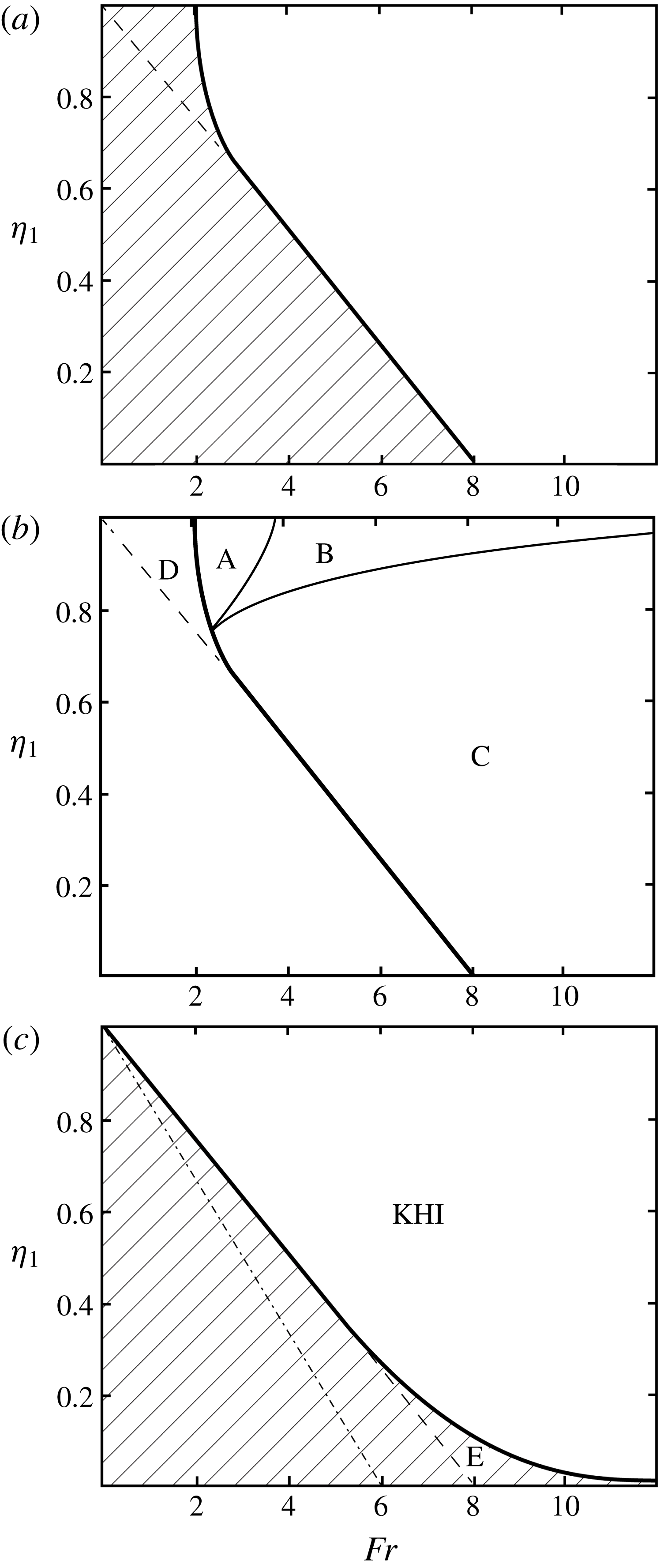
The stability of the upstream flow was examined by TL (their § 2.2) and is summarized in figure 2(c). The hatched region shows where KHI is not possible in the upstream flow, i.e. where the Taylor–Goldstein equation describing the stability of small perturbations to the flow has no exponentially growing solutions. KHI may occur in the remaining region of the ( $\unicode[STIX]{x1D702}_{1},Fr$ ) plane. A value $\mathit{Ri}_{1}=1/3$ corresponds to the dot-dashed line, $\mathit{Fr}=6(1-\unicode[STIX]{x1D702}_{1})$ . Points on this line are to the left of, and outside, the supercritical regions B and C of figure 2(b) in which hydraulic jumps are possible: it follows that a steady downstream flow with Richardson number $\mathit{Ri}_{2}=1/3$ is therefore stable both to KHI and to a possible hydraulic transition whatever the value $\unicode[STIX]{x1D702}_{2}$ . To be consistent with the model’s assumption that $\mathit{Ri}_{2}=1/3$ , a measured downstream Froude number should lie on (or at least be close to) the dotted line and be approximately equal to $6(1-\unicode[STIX]{x1D702}_{2})$ . Although, by comparing figure 2(b,c), it is evident that KHI is possible where jumps may occur in all of region B and most of C, there is a small region marked E in figure 2(c), part of C, where jumps are possible but KHI is not. (The flow with small values of $\unicode[STIX]{x1D702}_{1}$ is stabilized by the presence of the rigid boundary at $z=0$ , reducing the critical Richardson number to values below $1/4$ .) The possibility of KHI where jumps occur in regions B and C implies that (unless the flow is in the region E) it might be difficult, if not impossible, when comparing model predictions to observations to distinguish between hydraulic transitions and those caused by KHI; the occurrence of turbulence and an associated change in flow profiles may be a consequence of a hydraulic transition or of KHI, and in this sense the two are synonymous. (It will, however, be shown in § 3 that in at least two cases the nature of the hydraulic transition is quite distinct from KHI.) In regions A and D of figure 2(b), the upstream flow is liable to KHI but not to a hydraulic jump, in D because upstream waves are possible (figure 2 a) and in A because no hydraulic jump solutions can be found; for flows in region A, small-amplitude KHI disturbances may grow, but no finite-amplitude hydraulic transition is possible.

There is one factor that may distinguish hydraulic jumps from KHI. Where they occur, the turbulent hydraulic jumps are stationary, their position fixed where the flow becomes supercritical, e.g. downstream of sills or constrictions in the width of channels. The conditions favouring the onset of KHI may similarly be determined by the topography, e.g. by its enhancement of shear. It is, however, a property of KHI that the disturbances following instability and developing into billows and subsequently turbulence propagate downstream at a speed within the range of the flow speeds, i.e. so that a critical level exists. The billows propagate at a speed between that of the upper layer (zero in the model) and that of the lower layer, $U_{1}$ , possibly causing the critical position from which they develop, i.e. where the flow becomes subject to KHI (and possibly supercritical), to pulsate slightly in its downstream location.

As explained further in § 3 (and shown later in figure 6), the TL model provides prediction of other quantities related to transitions. The theory does not establish, however, the physical processes leading to the onset of turbulence in the transition. These might include an overturning billow-like structure or rotor (Ogden & Helfich Reference Ogden and Helfich2016; e.g. their figure 4d of an internal bore) or KHI. Nor does the theoretical model describe the nature of the flow within the turbulent transition (although it has been supposed to have a character sufficiently far downstream where turbulence has collapsed similar to that following KHI, with $\mathit{Ri}_{2}=1/3$ ). Much about its structure is, however, revealed by observations described in § 3. The model does not predict the values of $\unicode[STIX]{x1D702}$ or $\mathit{Fr}$ within the turbulent transition region itself, but these are determined from the observations. Some information is, however, available from the model about the mean rate of dissipation of turbulent kinetic energy as explained later, and estimates may be made of the vertical fluxes within the transition (Thorpe Reference Thorpe2010).

Figure 3.

Contours of potential temperature ( $^{\circ }\text{C}$ ) and stippled regions in which the rate of dissipation of turbulent kinetic energy per unit mass computed using Thorpe scales exceeds $10^{-7}~\text{W}~\text{kg}^{-1}$ in a section through the Samoan Passage made while steaming at low speed in tow-yo mode (from Alford et al. (Reference Alford, Girton, Voet, Carter, Mickett and Klymak2013), figure 3c). The bottom topography is shown in black. The two sections, 19–25 km and 3–12 km (i.e. $x=19$ –25 and 3–12), selected for analysis in §§ 3.2 and 3.3, respectively, are marked on the horizontal distance axis.

Observations are used in §§ 3–5 to examine the predictions (and test the validity) of the theoretical model. Assumptions and approximations made in applying the theoretical model to observations are reviewed in appendix B. One of these is that, rather than the uniform density of the $\unicode[STIX]{x1D702}$ profiles, the observed density profiles may have a nearly constant gradient above the flowing layer near the seabed (e.g. as seen later in profiles in figure 4 a). It is shown in appendix C that this appears unlikely to allow upward radiation of internal waves with energy and momentum loss from a transition region.

3 The Samoan Passage

3.1 The observations

Alford et al. (Reference Alford, Girton, Voet, Carter, Mickett and Klymak2013) examined the dense deep northerly flow through the Samoan Passage. They made detailed ‘tow-yo’ measurements with a conductivity–temperature–depth (CTD) probe and a lowered acoustic Doppler current profiler (LADCP) to obtain profiles of potential density (sigma4, referenced to 4000 m) and velocity in a region of mean depth of approximately 5100 m. The ‘tow-yo’ cycled between 40 m off the bottom and 4200 m depth, making profiles with a derived 1 m vertical resolution approximately 250 m apart, and thus inclined at a mean angle to the horizontal of approximately $74^{\circ }$ . Potential temperature and dissipation data over a major sill near $8^{\circ }$  S are displayed in figure 3(c) in Alford et al.’s paper and are reproduced here in figure 3. Being at low latitude, the effects of the Earth’s rotation are likely to be relatively small. This section shows locations designated by their position, $x$ (in kilometres), from 0 to 31.5. It passes in a northerly direction from just upstream (south) of the sill. Adjacent to the seabed an approximately 250 m thick layer of relatively dense water flows northwards at ${\sim}0.4~\text{m}~\text{s}^{-1}$ . It is capped by an interfacial layer in which the velocity and potential density decrease upwards. Above this, the flow is relatively small. The analysis made here is of two subsections of the data where hydraulic transitions appear likely. Section 3.2 describes $x=19$ to 25, presented first because (as it appears from figure 3) it is found to contain a single ‘cleanly defined’ hydraulic jump and consequently sets a standard for later analysis. Section 3.3 is from $x=3$ to 12 where a jump may also occur.

Figure 4.

Profiles of (a)  $\unicode[STIX]{x1D6F4}$ , the potential density, measured in $\text{kg}~\text{m}^{-3}$ , minus $1045.9~\text{kg}~\text{m}^{-3}$ , and (b) northward velocity, $u$ , in $\text{m}~\text{s}^{-1}$ , in the Samoan Passage at roughly 1 km intervals from approximately $x=19$ to $x=25$ . (The actual positions, the mean locations of the two-yo profiles, are $x=19.1$ , 20.1, 21, 22, 23.1, 24.1 and 25.2.) Successive profiles are displaced to the right by (a)  $0.2~\text{kg}~\text{m}^{-3}$ and (b)  $0.15~\text{m}~\text{s}^{-1}$ . The water depth is indicated by horizontal bars beneath each profile. The position of $u=0$ for each profile is marked at the top of (b) by vertical arrows. The features marked A to D in (a) are discussed in the text.

Additional measurements in the Samoan Passage are described by Voet et al. (Reference Voet, Girton, Alford, Carter, Klymak and Mickett2015, Reference Voet, Alford, Girton, Carter, Mickett and Klymak2016).

3.2 The tow-yo section from 19 to 25 km

Profiles of potential density and northwards velocity at 1 km spacing in the section of increasing depths from $x=19$ to $x=25$ are shown in figures 4(a) and 4(b), respectively. Table 1 shows the results of fitting the $\unicode[STIX]{x1D702}$ profiles to these data as described in appendix A. Here $\unicode[STIX]{x1D702}$ (with no subscript) is derived from the best fit of an $\unicode[STIX]{x1D702}$ profile to the observations at a position, $x$ . The mean thickness, $\unicode[STIX]{x1D702}h$ , of the lower layer is 256 m and its mean northward speed is $0.43~\text{m}~\text{s}^{-1}$ . The mean thickness of the interfacial layer is 274 m. With the estimated values of Fr and $\unicode[STIX]{x1D702}$ , figure 2 (with $\unicode[STIX]{x1D702}_{1}=\unicode[STIX]{x1D702}$ ) is used to determine whether or not the flow at various positions, $x$ , can support a hydraulic jump. Points in the ( $Fr,\unicode[STIX]{x1D702}$ ) plane denoted by their position, $x$ , are shown in figure 5(a), which is divided as in figure 2. At $x=19$ , the Froude number, $\mathit{Fr}=2.1$ and $\unicode[STIX]{x1D702}=0.64$ , and (from figure 2 b) the flow is subcritical (i.e. no hydraulic jump is possible). At $x=20$ , $\mathit{Fr}=4.7$ and $\unicode[STIX]{x1D702}=0.64$ and, as shown by the location of the point in figure 5(a), according to the model the flow is supercritical with (figure 2 b) a single solution for the downstream flow. The density profile contains few regions of static instability and there is a relatively low dissipation rate (figure 3).

Figure 5.

Values of $\unicode[STIX]{x1D702}$ and Fr at numbered kilometre locations in the Samoan Passage (a)  $x=19$ –25 and (b)  $x=3$ –12. Points to the right of the bold line are supercritical, those to the left subcritical. The uncertainties in observed values of $\unicode[STIX]{x1D702}$ and Fr are shown by error bars. The dot-dashed line corresponds to an interfacial gradient Richardson number of  $1/3$ .

Figure 6.

The model’s predictions of (a) the downstream profile parameter, $\unicode[STIX]{x1D702}_{2}$ , (b) the ratio of flowing layer thickness, $q=h_{2}/h_{1}$ , and (c) the non-dimensional energy loss, $E_{n}$ , in the ( $\unicode[STIX]{x1D702}_{1},Fr$ ) plane. Values of (upstream) $\unicode[STIX]{x1D702}_{1}$ and Fr are indicated at labelled locations, $x=4.8$ and 20 in the Samoan Passage where, according to the model, the flow becomes supercritical.

Table 1.

Values derived from fitting $\unicode[STIX]{x1D702}$ profiles to data at locations of $x=19$ to 25 in the Samoan Passage. The possible errors in the estimates of $\unicode[STIX]{x1D702}$ and Fr (and of $h$ and Ri at $x=22$ and 23) are indicated by ‘ $\pm$ ’ or a range of values. Locations where the range of possible values crosses the subcritical–supercritical boundary are labelled ‘uncertain’.

Figure 6 (reproduced from TL’s figure 5) shows contours of various downstream quantities derived from the model corresponding to upstream values, $\unicode[STIX]{x1D702}_{1}$ and Fr. The predicted downstream values (at a location where $\mathit{Ri}\sim 1/3$ ) that correspond to upstream values $\unicode[STIX]{x1D702}_{1}$ and Fr at $x=20$ are $\unicode[STIX]{x1D702}_{2}=0.47$ (figure 6 a) and $q=h_{2}/h_{1}=1.29$ (figure 6 b). The latter has $q>1$ and implies that the thickness of the overall flowing layer at the downstream location should exceed that upstream or, since at $x=20$ the layer thickness is $h_{1}=426~\text{m}$ (table 1), the predicted downstream value is $h_{2}=549~\text{m}$ . Moreover, the predicted downstream thickness of the lower layer, $\unicode[STIX]{x1D702}_{2}h_{2}$ , is 258 m, i.e. the thickness of the uniform layer below the interfacial layer should be less than that upstream, $\unicode[STIX]{x1D702}_{1}h_{1}=271~\text{m}$ . Since the upper edge of the interfacial layer is predicted to increase in height above the bottom and the lower edge to decrease, a mode 2 transition from upstream to downstream of the transition is expected as noted in § 2. But, to comply with the model, does the flow attain an approximately steady subcritical state with $\mathit{Ri}_{2}\approx 1/3$ at some $x>20$ ?

Although there is a well-defined shear and density interface between 4670 and 4790 m depth at $x=21$ , above it the density profile has a large region of static instability with variable shear at depths of 4530–4700 m, marked ‘A’ in figure 4(a), and this $x$ location (the parameters of the interfacial region also implying in figure 5(a) that the flow is supercritical) is presumably within a hydraulic jump downstream of $x=20$ following its supercritical state. At $x=22$ there is a near-uniform layer from 4520 to 4750 m, marked ‘B’ in figure 4(a), containing a 60 m high region of static instability. At $x=23$ , there is what appears to be an 80 m deep layer of residual overturn, marked ‘C’, near 4650 m. Evidence of this mixing region persists at $x=24$ , marked ‘D’. The presence of the inversions (statically unstable regions) is reflected by the large uncertainty in Fr shown in table 1 and figure 5(a) at $x=22$ and 23, and consequently the sub- or supercritical state of the flow is not definitely known at $x=22$ , although the latter is favoured. However, at $x=24$ the flow becomes subcritical (although the interfaces in both density and velocity are somewhat irregular, possibly layered) with $\mathit{Ri}=0.33~({\approx}1/3)$ and a Froude number that approaches the dot-dashed line in figure 2(c), reproduced in figure 5(a), as required in the model flow downstream of KHI.

The features of the jump described in the last paragraph are illustrated in more detail in the potential density contours of figure 7. The mixing region is outlined by an oval-shaped curve to indicate its location and approximate dimensions. It is characterized by relatively uniform density but with frequent inversions. It begins near $x=20$ , the position where the flow is first predicted to be supercritical. The mixing region appears initially near 4600 m depth, approximately 410 m off the bottom, splitting into two the upstream stratified interfacial layer between 4530 and 4650 m. The potential density of the fluid where the mixed layer first appears is slightly less than the mean potential density in this interfacial layer. At $x=22$ the layer develops into a vertically near-uniform region containing frequent density inversions extending from 4480 to 4770 m depth. At $x=23$ , the centre of the mixing region is at 4650 m, approximately 485 m off the bottom. The density of the oval-shaped mixing region increases with $x$ as more dense water is entrained from the bottom layer. Overall the layer of mixing resembles a mid-water (i.e. separated by approximately 200 m from the bottom) 3.7 km long rotor-like structure following the gradual bottom slope, although no significant sustained flow in the upstream direction was recorded that might confirm the circulatory flow of a rotor. At its maximum the mixing layer is approximately 390 m in height, and its aspect ratio – height divided by length – is approximately 0.08. The velocity field is more uncertain and less firmly structured than the density, but the oval layer appears to have a generally weak flow above its stratified base below which the near-bed northerly flow continues at approximately $0.4~\text{m}~\text{s}^{-1}$ . The mixing layer forming the hydraulic jump has a form reminiscent of a steady spilling surface-wave breaker (e.g. Rapp & Melville (Reference Rapp and Melville1990)), like that downstream of a weir led by a ‘toe’ near $x=20$ , $z=4600~\text{m}$ . There is no evidence that it is initiated by an overturn caused by convective instability (as in a plunging surface-wave breaker) or by KH billows, characterized, for example, by ‘braids’, high-gradient regions between periodic billows, although the uniformity of the layer is sustained by static instability and convection. Its form is similar to that produced by breaking forced internal waves in the atmosphere above mountain ridges, modelled by Afanasyev & Peltier (Reference Afanasyev and Peltier1998, see especially their figure 12d) and by Yakovenko, Thomas & Castro (Reference Yakovenko, Thomas and Castro2011).

Figure 7.

Contours of potential density at intervals of $5\times 10^{-3}~\text{kg}~\text{m}^{-3}$ between $x=19.1$ and $x=24.1$ and depths ranging from 4400 to 4900 m in the Samoan Passage. The mean horizontal locations of vertical profiles made by the tow-yo are indicated by dots on the $x$ -axis. The flow becomes supercritical at $x\approx 20$ . The approximate position of the mixing region associated with the hydraulic jump is indicated by the oval-shaped curve. The step-like structure of the unsmoothed contours sloping downwards from $x=19.1$ , $z=4680~\text{m}$ is probably unreal, a consequence of interpolation by the computer package used to construct the contours as a narrow density interface moves downwards as $x$ increases.

The values of $\unicode[STIX]{x1D702}$ and $h$ at $x=24$ are 0.33 and 561 m, respectively, compared to the model’s predicted values of 0.47 and 549 m, respectively, for a jump produced by the flow at $x=20$ . The lower layer thickness at $x=24$ is 186 m, less than the predicted 258 m, but at least showing that the transition is of mode 2, as predicted. In view of the assumptions made in the theoretical model, of the uncertainty in fitting the $\unicode[STIX]{x1D702}$ profiles to data (reflected in the error bars of figure 5 a), of whether the profiles at $x=20$ represent the flow conditions immediately before the transition, and of the unaccounted-for variations in bottom topography shown in figure 3 over the horizontal extent of the transition layer shown in figure 7, it is not surprising that the predicted values differ somewhat from the observed. The density within the interfacial layer is irregular and ‘step-like’ at $x=25$ (figure 4 a). At this location, however, the northward velocity of the flow above the interfacial layer is approximately $0.1~\text{m}~\text{s}^{-1}$ , violating the model’s assumption of zero flow.

Contours of a non-dimensional energy loss in the jump, $E_{n}$ , in ( $Fr,\unicode[STIX]{x1D702}_{1}$ ) space, estimated by TL (their equation (4.3)), are given by figure 6(c). The value of $E_{n}$ is related to the mean rate of dissipation of turbulent kinetic energy per unit mass in the hydraulic jump, $\unicode[STIX]{x1D700}$ , by

(3.1) $$\begin{eqnarray}\unicode[STIX]{x1D700}=E_{n}U_{1}^{3}(1+3\unicode[STIX]{x1D702}_{1})/\{4L_{j}[(1-\unicode[STIX]{x1D702}_{1})+q(1-\unicode[STIX]{x1D702}_{2})]\},\end{eqnarray}$$

where $L_{j}$ is the horizontal extent of the transition region associated with the hydraulic jump, $q=h_{2}/h_{1}$ , and $U_{1}$ ( ${\approx}0.43~\text{m}~\text{s}^{-1}$ ) is the speed of the lower layer upstream of the jump. Using the upstream values of $\unicode[STIX]{x1D702}_{1}$ and Fr at $x=20$ , figure 6(c) gives $E_{n}\approx 0.035$ . Selecting the downstream value of $\unicode[STIX]{x1D702}_{2}$ as that at $x=24$ , and choosing $L_{j}=4~\text{km}$ (the separation distance between the upstream and downstream locations) gives a mean value, $\unicode[STIX]{x1D700}=4.1\times 10^{-7}~\text{W}~\text{kg}^{-1}$ . This is comparable to the values observed and given in Alford et al.’s figures 2 and 3(c), the latter reproduced here in figure 3. A further comparison of theory and data is made in appendix D: the approximate time required for turbulence to collapse is consistent with the observations of the length of the active mixing region estimated to be approximately $6U_{1}N^{-1}$ , where $N$ is the mean buoyancy frequency of the stratified region surrounding the upstream interfacial layer.

In summary, a transition begins at $x=20$ , the location where, according to the model, the flow becomes supercritical, and it takes the form of an elongated mixing layer. If this is a rotor, it is similar to those found in numerical studies of moving bores by Ogden & Helfich (Reference Ogden and Helfich2016). It is separated from the seabed by a relatively strong downslope bottom flow, and thus differs from the near-boundary rotors found in large internal waves in the lee of mountains described by Scorer (Reference Scorer1955, Reference Scorer1972, e.g. his Reference Scorer1972 figure 5.7i) and Doyle & Durran (Reference Doyle and Durran2007). No KH billows or braids are apparent in the tow-yo profiles immediately downstream of $x=20$ .

3.3 The tow-yo section from 3 to 12 km

Table 2 and figure 5(b) show the results of fitting the $\unicode[STIX]{x1D702}$ profiles to data in $3\leqslant x\leqslant 12$ . The mean thicknesses, the averages of $\unicode[STIX]{x1D702}h$ and $h$ of the other flowing layers between $x=3$ and $x=12$ , are 283 and 484 m, respectively, and the mean northward speed of the dense lower layer is $0.30~\text{m}~\text{s}^{-1}$ . However, at $x=7$ , the flow is unusually small, less than $0.05~\text{m}~\text{s}^{-1}$ , throughout the depth range sampled by the tow-yo. Although the density profile was ‘normal’, with a well-defined interfacial layer between depths of approximately 4300 and 4700 m, no northward-going lower layer appears in the velocity profile. We have no simple explanation for this and it was not possible to fit consistent $\unicode[STIX]{x1D702}$ profiles to both velocity and density.

Table 2.

Values derived from fitting $\unicode[STIX]{x1D702}$ profiles to data at locations of $x=3$ to 12 in the Samoan Passage. The uncertainty in the estimates of $\unicode[STIX]{x1D702}$ and Fr are indicated by ‘ $\pm$ ’. At $x=7$ (marked $\ast$ ), the flow is small, less than $0.1~\text{m}~\text{s}^{-1}$ , perhaps being blocked, and it was not possible to fit consistent $\unicode[STIX]{x1D702}$ profiles to both velocity and density. At $x=9$ the flow is marginal (i.e. on or very close to the supercritical–subcritical boundary in figure 4 b) although unstable to KHI.

According to the model the flow becomes supercritical at $x=4.8$ , returning to subcritical at $x=5.8$ . As shown in the contours of potential density in figure 8 a 100 m high structure with numerous density inversions outlined by the oval-shaped curve appears in the flow at $x=4.8$ . Its density is approximately equal to the mean of that in the upstream interfacial layer and it divides this layer into two. This mixing region extends approximately 1 km downstream, ending at $x\approx 5.8$ , the location at which the flow returns to a subcritical state. The aspect ratio of the mixing region is approximately 0.1 compared with 0.08 for the transition at $x=20$ shown in figure 7. Its length as predicted in appendix D is $6U_{1}N^{-1}\approx 1.5~\text{km}$ rather than the 1 km observed. Other mixing layers appear beyond $x=5.8$ , e.g. near $x=6.1$ , $z=4680~\text{m}$ , where, according to the model, the flow is subcritical but downstream of substantial increases in water depth.

Figure 8.

Contours of potential density at intervals of $5\times 10^{-3}~\text{kg}~\text{m}^{-3}$ through the hydraulic jump between $x=4$ and $x=7$ below 4300 m depth in the Samoan Passage. The mean horizontal locations of vertical profiles made by the tow-yo and the depth of the seabed are indicated by the dots. Tow-yo profiles extend only to approximately 40 m from the seabed so no data are available closer to the seabed. The flow becomes supercritical at $x\approx 4.8$ . The approximate position of the oval-shaped mixing region associated with the hydraulic jump is outlined.

Using the values of $\unicode[STIX]{x1D702}$ and Fr at $x=4.8$ as those upstream of a transition, figure 6(a) predicts $\unicode[STIX]{x1D702}_{2}\approx 0.57$ downstream. This compares fairly well with the observed value, 0.53, at the subcritical downstream end of the mixed structure at $x=5.8$ . The Richardson number at $x=5.8$ is, however, 0.48, indicating a stable flow, but greater than the value, $\mathit{Ri}_{2}=0.33$ , adopted in the model. The value of $E_{n}$ determined from figure 6(c) at $x=4.8$ is approximately 0.018. The mean value of $\unicode[STIX]{x1D700}$ in the 1 km between $x=4.8$ and 5.8 derived using (3.1) is approximately $1.0\times 10^{\text{-6}}~\text{W}~\text{kg}^{-1}$ , in order-of-magnitude accord with the values shown in figure 3. Although smaller than the feature associated with the hydraulic jump at $x=20$ , the mixed structure shares many of its general characteristics, including its being separated from the seabed by the near-bottom northerly flow of dense water and by an absence of any clear evidence of KH billows or braids.

4 The Red Sea Outflow

A different Froude number, described as a ‘bulk Froude number’ and denoted here by $\mathit{Fr}_{P}$ , is used by Peters et al. (Reference Peters, Johns, Bower and Fratantoni2005) in the analysis of data from the Red Sea Outflow in the Gulf of Aden, a near-bottom flow with velocity and density structure similar to the profiles considered in the Samoan Passage. In terms of the notation of § 2, Peters et al. define $\mathit{Fr}_{P}$ ‘following discussion with Price 2003 (personal communication)’ by

(4.1) $$\begin{eqnarray}\displaystyle \mathit{Fr}_{P}^{2} & = & \displaystyle (U_{1}/2)^{2}/\{g\unicode[STIX]{x1D6E5}[\unicode[STIX]{x1D702}_{1}h_{1}+h_{1}(1-\unicode[STIX]{x1D702}_{1})/2]\},\nonumber\\ \displaystyle & = & \displaystyle U_{1}^{2}/[2g\unicode[STIX]{x1D6E5}h_{1}(1+\unicode[STIX]{x1D702}_{1})],\end{eqnarray}$$

or, in terms of Fr given by (2.5) and the local value, $\unicode[STIX]{x1D702}_{1}$ ,

(4.2) $$\begin{eqnarray}\mathit{Fr}_{P}^{2}=\mathit{Fr}/[2(1+\unicode[STIX]{x1D702}_{1})].\end{eqnarray}$$

The critical curves in the ( $\unicode[STIX]{x1D702}_{1},Fr$ ) plane shown in figure 2 are translated to the ( $\unicode[STIX]{x1D702}_{1},Fr_{P}$ ) plane in figure 9. The thick line represents the lowest values of $\mathit{Fr}_{P}$ at which, according to the model described in § 2, a hydraulic transition can occur for given $\unicode[STIX]{x1D702}_{1}$ ; values of the minimum $\mathit{Fr}_{P}$ vary with $\unicode[STIX]{x1D702}_{1}$ . The smallest $\mathit{Fr}_{P}$ at which transition can occur is 0.80 at $\unicode[STIX]{x1D702}_{1}=0.74$ . The minimum (or critical) $\mathit{Fr}_{P}$ is equal to unity only when $\unicode[STIX]{x1D702}_{1}=0.6$ .

Figure 9.

The critical curves of figure 2 translated to the $(\unicode[STIX]{x1D702}_{1},\mathit{Fr}_{P})$ plane. Regions A–E correspond to those in figure 2(b,c). The thick line represents the lowest values of $\mathit{Fr}_{P}$ at which a hydraulic transition can occur for given $\unicode[STIX]{x1D702}_{1}$ . In (a) points are taken from Peters & Johns (Reference Peters and Johns2005) in the two channels, NC and SC, of the Red Sea Outflow. In (b) points are taken from Gasser et al. (Reference Gasser, Pelegi, Nash, Peters and Garcia-Lafuente2011) and Nash et al. (Reference Nash, Peters, Kelly, Pelegri, Emelianov and Gasser2012) at stations UTS and DTS in the Mediterranean Outflow. The dot-dashed line corresponds to an interfacial gradient Richardson number of  $1/3$ .

The Red Sea Outflow exits the Red Sea through the Strait of Bab el Mandeb and passes down two channels in the Gulf of Aden between $12^{\circ }\,\text{N}$ and $12^{\circ }30^{\prime }\,\text{N}$ , the northern and southern channels denoted by Peters et al. (Reference Peters, Johns, Bower and Fratantoni2005) as NC and SC, respectively. The outflow, confined to the channels, is conceived by Peters & Johns (Reference Peters and Johns2005) and Peters et al. (Reference Peters, Johns, Bower and Fratantoni2005) in terms of gradually entraining plumes of dense water rather than gravity currents and in which the spread is dominated by localized hydraulic jumps. Measurements are made using a package combining an LADCP and CTD. During the period of stronger flow in observations made in winter, values of $\mathit{Fr}_{P}$ estimated by Peters & Johns (Reference Peters and Johns2005) have locally maximum values of approximately 0.93 and 0.97 at down-channel distances in the NC of approximately 70 and 120 km, respectively, from the Strait of Bab al Mandeb, and 0.88 at approximately 60 km in the SC. At all three locations, the rate of dissipation of turbulent kinetic energy, estimated using an assumed proportionality between the Ozmidov and Thorpe length scales, is also maximal, suggesting the possible presence of hydraulic jumps. At these locations the value $\unicode[STIX]{x1D702}_{1}$ , taken here as the ratio of the bottom layer to the total thickness of the flowing layer ( $H_{b}/H_{p}$ in the notation of Peters & Johns (Reference Peters and Johns2005)) is approximately 0.30 and 0.27 in the NC, and 0.42 in the SC. The corresponding points in the ( $Fr_{P},\unicode[STIX]{x1D702}_{1}$ ) plane are shown in figure 9(a) and indicate that, although the values of $\mathit{Fr}_{P}$ exceed the minimum for hydraulic jumps to occur, the flows should be subcritical, stable to hydraulic jumps at the estimated $\unicode[STIX]{x1D702}_{1}$ . Values are, however, uncertain. Peters & Johns (Reference Peters and Johns2005) and Peters et al. (Reference Peters, Johns, Bower and Fratantoni2005) take the depth of the lower layer ( $\unicode[STIX]{x1D702}h$ , or $H_{b}$ in their notation) as the height above the seabed at which the downstream velocity is a maximum, less than the estimate of $\unicode[STIX]{x1D702}_{1}h$ determined as in appendix A. The total thickness of the flowing layer ( $H_{p}$ in their notation) is taken in a less precise way, depending on the speed or direction of the velocity, or on the salinity. The value $\unicode[STIX]{x1D702}_{1}=H_{b}/H_{p}$ is likely to be less than that found in appendix A, and $\mathit{Fr}_{P}$ may consequently be overestimated. There is no clear evidence from observations or theory of the presence of hydraulic jumps in the Red Sea Outflow. Rather, the spreading of the outflow down the channels in the Gulf of Aden appears to be dominated by a more gradual process of turbulent entrainment as concluded by the two sets of authors.

5 The Mediterranean Outflow

Gasser et al. (Reference Gasser, Pelegi, Nash, Peters and Garcia-Lafuente2011) and Nash et al. (Reference Nash, Peters, Kelly, Pelegri, Emelianov and Gasser2012) report observations using moorings and tow-yos in the Mediterranean Outflow in the Gulf of Cadiz 70 km west of the Strait of Gibraltar and to the west of the Espartel Sill, the most western sill of the Strait. At this location the dense outflow is confined to a westward-flowing layer of water, some 150 m thick and of relatively high salinity, moving westward over the seabed at approximately $1.2~\text{m}~\text{s}^{-1}$ . Profiles of density and velocity are derived from the surface to the bottom with 1 km horizontal resolution. Flow in the layer overlying the outflow is of order $0.2~\text{m}~\text{s}^{-1}$ to the east. Gasser et al. (Reference Gasser, Pelegi, Nash, Peters and Garcia-Lafuente2011) show roughly 10 km long downstream tow-yo sections of salinity, downstream velocity and gradient Richardson number at four stages of the $M_{2}$ tidal cycle. Nash et al. (Reference Nash, Peters, Kelly, Pelegri, Emelianov and Gasser2012) present a tow-yo section of downstream velocity and $\log \unicode[STIX]{x1D700}$ at the same time as that of the low tidal flow section presented by Gasser et al., and focus attention on two stations in the section, separated by approximately 3.5 km, UTS (upstream at $6^{\circ }19.23^{\prime }\,\text{W}$ , $35^{\circ }47.04^{\prime }\,\text{N}$ , where the water depth is approximately 417 m) and DTS (downstream at $6^{\circ }21.00^{\prime }\,\text{W}$ , $35^{\circ }46.51^{\prime }\text{N}$ , in 454 m).

Following Peters et al. (Reference Peters, Johns, Bower and Fratantoni2005), Nash et al. (Reference Nash, Peters, Kelly, Pelegri, Emelianov and Gasser2012) use the bulk Froude number, $\mathit{Fr}_{P}$ , in their analysis, but assume, without formal justification, that transition occurs at $\mathit{Fr}_{P}=1$ . At UTS, 90 % of the estimates of $\mathit{Fr}_{P}$ lie between 0.70 and 0.92 (with a mean of 0.81). The mean dissipation, $\unicode[STIX]{x1D700}$ , in the outflowing layer is approximately $1\times 10^{-6}~\text{W}~\text{kg}^{-1}$ . The value of $\unicode[STIX]{x1D702}$ estimated from the profiles given by Gasser et al. (Reference Gasser, Pelegi, Nash, Peters and Garcia-Lafuente2011) and Nash et al. (Reference Nash, Peters, Kelly, Pelegri, Emelianov and Gasser2012) is $0.45\pm 0.03$ . Respective points are shown in figure 9(b). They indicate that, according to the model, the flow is subcritical and stable to a hydraulic transition at UTS.

Approximately 1–2 km west of UTS Nash et al. (Reference Nash, Peters, Kelly, Pelegri, Emelianov and Gasser2012, their figure 3b,c) find a notable increase in the high-frequency displacement of isopycnals, an increase in interface thickness and a rise in $\unicode[STIX]{x1D700}$ to a mean value of approximately $1\times 10^{-5}~\text{W}~\text{kg}^{-1}$ in the outflow, suggesting that a mode 2 transition has occurred. Further downstream at DTS the mean $\mathit{Fr}_{P}=0.99$ and 90 % of the estimates of $\mathit{Fr}_{P}$ lie between 0.63 and 1.45, 45 % having $\mathit{Fr}_{P}>1$ , and $\unicode[STIX]{x1D702}$ is equal to $0.39\pm 0.03$ . As shown in figure 9(b), the upper values of these estimates of $\mathit{Fr}_{P}$ and $\unicode[STIX]{x1D702}$ imply that a hydraulic jump is possible. It is likely, however, that conditions for a jump have been reached upstream of DTS and that DTS lies within the transitional region, this accounting for the relatively large variations in isopycnal depths and in $\mathit{Fr}_{P}$ or $\mathit{Fr}$ . Similarly large variations in $\mathit{Fr}$ are observed downstream of the hydraulic jump at $x=20$ –21 in the Samoan Passage (figure 5 a). (Taking the upper values at DTS, $\mathit{Fr}_{P}\approx 1.45$ and $\unicode[STIX]{x1D702}\approx 0.4$ , we find $\mathit{Fr}=5.85$ from (4.2) while figure 6 gives $\unicode[STIX]{x1D702}_{2}\approx 0.3$ , $q\approx 0.8$ and $E_{n}\approx 0.05$ . Taking $L_{j}$ equal to the distance between the two stations, i.e. 3.5 km, and using (3.1), gives $\unicode[STIX]{x1D700}\approx 1.2\times 10^{-5}~\text{W}~\text{kg}^{-1}$ , consistent with the observed dissipation rate at DTS.) Nash et al. (Reference Nash, Peters, Kelly, Pelegri, Emelianov and Gasser2012) use the Taylor–Goldstein equation to examine the stability of the flow at DTS to KHI. The gradient Richardson number of the flow near the centre of the interface above the flowing layer is less than $1/4$ , and the flow is found to be unstable to KHI, consistent with the larger values of $\mathit{Fr}_{P}$ being in region C of figure 9(b). Downstream (to the west) of DTS the depth of the seabed increases sharply to approximately 500 m, resulting in an increase of $\unicode[STIX]{x1D702}$ to approximately 0.5, a flow that exhibits 30–50 m overturns and $\unicode[STIX]{x1D700}$ exceeding $10^{-5}~\text{W}~\text{kg}^{-1}$ , again suggestive of a hydraulic jump.