1 Introduction
Shear-induced diffusion underpins the mixing of grains in a variety of geophysical and industrial granular flows. When intergranular cohesive forces are small or null, the shear-induced diffusivity
 $D$
can be expressed in terms of the grain size
 $d$
and the mean grain velocity fluctuation
 $\unicode[STIX]{x1D6FF}v$
(Zik & Stavans Reference Zik and Stavans1991; Natarajan, Hunt & Taylor Reference Natarajan, Hunt and Taylor1995; Hsiau et al.
Reference Hsiau, Lu, Chou and Yang2008; Kharel & Rognon Reference Kharel and Rognon2017):
 $$\begin{eqnarray}D\propto d\unicode[STIX]{x1D6FF}v.\end{eqnarray}$$
This scaling is consistent with an elementary grain trajectory following a random walk of step
 $d$
and frequency
 $\unicode[STIX]{x1D6FF}v/d$
. In confined flows where the solid fraction is fixed, velocity fluctuations depend on the shear rate
 $\dot{\unicode[STIX]{x1D6FE}}$
(Losert et al.
Reference Losert, Bocquet, Lubensky and Gollub2000; Pouliquen & Chevoir Reference Pouliquen and Chevoir2002; Mueth Reference Mueth2003), the grains’ size, and a function of the solid fraction
 $f(\unicode[STIX]{x1D719})$
(Campbell Reference Campbell1997; Hsiau & Shieh Reference Hsiau and Shieh2000; Gross, Krüger & Varnik Reference Gross, Krüger and Varnik2015):
 $\unicode[STIX]{x1D6FF}v\propto \dot{\unicode[STIX]{x1D6FE}}df(\unicode[STIX]{x1D719})$
. The diffusivity can be then be expressed as:
 $D=d^{2}\dot{\unicode[STIX]{x1D6FE}}f(\unicode[STIX]{x1D719})$
(Natarajan et al.
Reference Natarajan, Hunt and Taylor1995; Utter & Behringer Reference Utter and Behringer2004; Hsiau et al.
Reference Hsiau, Lu, Chou and Yang2008). In contrast, in flows where normal stresses are fixed and dilatancy is possible, velocity fluctuations can be expressed as a function of the inertial number
 ${\mathcal{I}}$
(defined in § 2) (Da Cruz et al.
Reference Da Cruz, Emam, Prochnow, Roux and Chevoir2005; DeGiuli, McElwaine & Wyart Reference DeGiuli, McElwaine and Wyart2016):
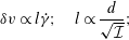 $$\begin{eqnarray}\unicode[STIX]{x1D6FF}v\propto l\dot{\unicode[STIX]{x1D6FE}};\quad l\propto \frac{d}{\sqrt{{\mathcal{I}}}};\end{eqnarray}$$
where
 $l$
is the typical cluster size of grains forming in the flow (Kharel & Rognon Reference Kharel and Rognon2017). Accordingly, the shear-induced diffusivity of cohesionless granular flow is given by:
 $$\begin{eqnarray}D\propto d^{2}\frac{\dot{\unicode[STIX]{x1D6FE}}}{\sqrt{{\mathcal{I}}}}.\end{eqnarray}$$
The effect of cohesion on shear-induced diffusivity in dense granular flows is poorly documented. What is known is that cohesion induces the formation of large clusters within the flows, which can be long-lived (Rognon et al.
Reference Rognon, Roux, Naaim and Chevoir2008). However, the effect of these clusters on the diffusivity has not been established. Open questions include: (i) does the scaling (1.1) hold in the presence of cohesion; (ii) how does cohesion influence the velocity fluctuation
 $\unicode[STIX]{x1D6FF}v$
and the scaling (1.2); and ultimately (iii) can the diffusivity scaling (1.3) be extended to cohesive grains?
The aim of this paper is to address these questions. Our approach consists of (i) measuring the grain diffusivity in simulated flows for different inertial numbers and different levels of cohesion and (ii) assessing and possibly extending the above scalings established for cohesionless grains to account for cohesion.
2 Measuring self-diffusivity in granular flows
According to (1.3), shear-induced diffusivity is expected to depend on the shear rate and possibly on the inertial number
 ${\mathcal{I}}$
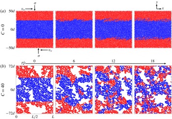
. We therefore opted to measure it in a flow geometry where these two quantities are homogeneous and can be tuned. Figure 1 illustrates this geometry, which is a plane shear with a prescribed shear rate
 $\dot{\unicode[STIX]{x1D6FE}}$
and normal stress
 $\unicode[STIX]{x1D70E}$
. A bi-periodic domain with Lees–Edwards-type boundary conditions is used to avoid walls and the shear heterogeneity they may induce. There is no gravity. Flows are simulated using a discrete element method, with specifics given in appendix A.
Simulated systems are bi-dimensional and contain
 $10^{4}$
elastic cylinders with mean grain diameter
 $d$
, depth
 $d$
and mean grain mass
 $m$
. These cylinders interact with their neighbours via elastic, dissipative, and frictional contacts, as well as a constant cohesive force of magnitude
 $f_{0}$
. This cohesive force acts on every contact, is normal to the contact, and is null when grains do not touch.
We characterise the flows and the intensity of cohesion using two non-dimensional numbers: the inertial number
 ${\mathcal{I}}$
(MiDi Reference MiDi2004; Da Cruz et al.
Reference Da Cruz, Emam, Prochnow, Roux and Chevoir2005) and the cohesion number
 $C$
(Gilabert, Roux & Castellanos Reference Gilabert, Roux and Castellanos2007; Rognon et al.
Reference Rognon, Roux, Naaim and Chevoir2008; Khamseh, Roux & Chevoir Reference Khamseh, Roux and Chevoir2015), defined as:
 $$\begin{eqnarray}{\mathcal{I}}=\dot{\unicode[STIX]{x1D6FE}}t_{i};\quad t_{i}=\sqrt{\frac{m}{\unicode[STIX]{x1D70E}d}};\quad C=\frac{f_{0}}{\unicode[STIX]{x1D70E}d^{2}}.\end{eqnarray}$$
The inertial number compares the shear time
 $\dot{\unicode[STIX]{x1D6FE}}^{-1}$
to the inertial time
 $t_{i}$
, which reflects a typical rearrangement time of an inertial grain driven by the normal stress
 $\unicode[STIX]{x1D70E}$
. The cohesion number compares the magnitude of the contact cohesion force to the force scale
 $\unicode[STIX]{x1D70E}d^{2}$
associated to the normal stress.
Grain mixing during shear (
 ${\mathcal{I}}=0.05$
) without cohesion (a) and with cohesion (b,
 $C=40$
). Snapshots are taken during the flow. Initially, grains located in the centre of the system are coloured in blue, and the rest in red. Grains keep their initial colour throughout the flow to help visualising the mixing process. Supplementary movies 1–4 available online at https://doi.org/10.1017/jfm.2018.861 show more examples of mixing at different inertial and cohesion numbers.

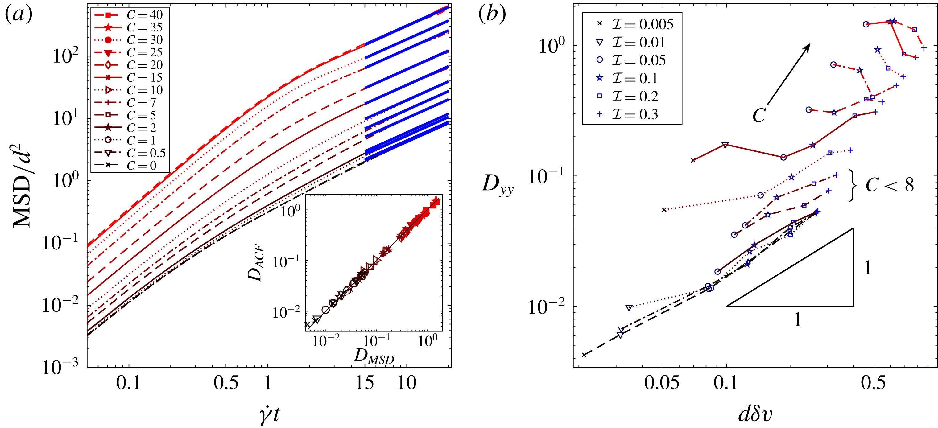
Coefficient of diffusion measured in plane shear flows at various
 ${\mathcal{I}}$
and
 $C$
. (a) Examples of MSD (
 ${\mathcal{I}}=0.1$
, different cohesion); the corresponding diffusivity is measured by fitting (2.2) (solid blue lines represent best fits). Inset: equivalence of the diffusivities (in units
 $d^{2}t_{i}$
) measured with the Einstein formula (
 $D_{MSD}$
, from (2.2)) with the Green–Kubo formula (
 $D_{ACF}$
, from (2.3)). The black line represents the identity function. (b) Measured diffusivity against velocity fluctuations (both in units
 $d^{2}t_{i}$
) at different
 ${\mathcal{I}}$
over level curves of cohesion. Linear relations exist only for
 $C<8$
. Legend for the lines is in (a).

We simulated a series of flows at different values of inertial numbers in the range
 $5\times 10^{-3}\leqslant {\mathcal{I}}\leqslant 0.3$
, which corresponds to the dense flow regime for cohesionless grains (MiDi Reference MiDi2004; Da Cruz et al.
Reference Da Cruz, Emam, Prochnow, Roux and Chevoir2005), and for different values of the cohesion number in the range
 $0\leqslant C\leqslant 40$
.
Each test involves initially seeding grains in a loose configuration without any contacts, and then applying the shear rate and normal stress until a steady state is reached. We observed that persistent shear bands could develop, especially at high values of
 $C$
and low values of
 ${\mathcal{I}}$
. Appendix A details how these shear bands were detected. In the following, flows featuring shear bands have been excluded from the analysis as the local shear rates and inertial numbers are then heterogeneous. The analysis focuses on flows that have reached a homogeneous steady state. In these flows, grain trajectories and velocities are recorded during a period of
 $t_{max}=22/\dot{\unicode[STIX]{x1D6FE}}$
, or 22 shear deformations.
The diffusivity of grains in the
 $y$
-direction – transverse to the shear – is measured from grain trajectories and velocities using two well-established methods.
The first method is based on Einstein’s theory that relates the diffusivity to the ensemble average
 $\langle \cdots \rangle$
of the mean squared displacement (MSD) of grains in the transverse direction
 $\unicode[STIX]{x0394}y^{2}$
(Natarajan et al.
Reference Natarajan, Hunt and Taylor1995; Dufty, Brey & Lutsko Reference Dufty, Brey and Lutsko2002; Sierou & Brady Reference Sierou and Brady2004):
 $$\begin{eqnarray}\langle \unicode[STIX]{x0394}y^{2}(t)\rangle =2tD_{yy}(t);\quad \unicode[STIX]{x0394}y(t)=y(t+t_{0})-y(t_{0}).\end{eqnarray}$$
The diffusivity is given by the long-term limit
 $D=\lim _{t\rightarrow \infty }D_{yy}(t)$
, although it is sufficient to consider
 $D_{yy}(t)$
at a finite time, provided it is linear in
 $t$
. We used the time invariance of our steady flows to compute the ensemble average robustly. For each lag time
 $0\leqslant t\leqslant 20\dot{\unicode[STIX]{x1D6FE}}$
, the diffusivity was computed not only over all the grains but also over every possible starting time, as detailed in appendix B. Figure 2 shows that the measured mean square displacement first exhibits a superdiffusive behaviour at short time scales (
 $\langle \unicode[STIX]{x0394}y^{2}(t)\rangle \propto t^{\unicode[STIX]{x1D6FD}}$
with
 $\unicode[STIX]{x1D6FD}>1$
), and then converges towards a normal-diffusive behaviour as per (2.2). Accordingly, diffusivities were extracted by fitting long-term MSD to (2.2), as illustrated in figure 2.
The second method is based on Green–Kubo’s formula that relates the diffusivity to velocity fluctuations of the grains and their time correlation. It can be derived from Einstein’s formula (2.2) by expressing grain displacements as a function of their velocity
 $v_{y}(t)$
as
 $\unicode[STIX]{x0394}y(t)=\int _{0}^{t}v_{y}(\unicode[STIX]{x1D70F})\,\text{d}\unicode[STIX]{x1D70F}$
and introducing the normalised velocity autocorrelation function
 $\unicode[STIX]{x1D713}(\unicode[STIX]{x1D70F})=\langle v_{y}(\unicode[STIX]{x1D70F})v_{y}(0)\rangle /\langle v_{y}^{2}(0)\rangle$
. This leads to
 $D_{yy}(t)=\unicode[STIX]{x1D6FF}v^{2}\int _{0}^{t}(1-(\unicode[STIX]{x1D70F}/t))\unicode[STIX]{x1D713}(\unicode[STIX]{x1D70F})\,\text{d}\unicode[STIX]{x1D70F}$
, with
 $\unicode[STIX]{x1D6FF}v^{2}\equiv \langle v_{y}^{2}(0)\rangle =\langle v_{y}^{2}\rangle -\langle v_{y}\rangle ^{2}$
. The Green–Kubo relation we use results from the limit of
 $t\rightarrow \infty$
. The diffusivity is then expressed as:
 $$\begin{eqnarray}D=\unicode[STIX]{x1D6FF}v^{2}\unicode[STIX]{x1D6F9};\quad \unicode[STIX]{x1D6F9}=\int _{0}^{\infty }\unicode[STIX]{x1D713}(\unicode[STIX]{x1D70F})\,\text{d}\unicode[STIX]{x1D70F};\end{eqnarray}$$
where
 $\unicode[STIX]{x1D6F9}$
is called the memory or Lagrangian time, and measures the typical correlation time of the velocity fluctuations. Appendix C details how this correlation is measured in our simulations.
In principle, both formulations (2.2) and (2.3) are equivalent as
 $t\rightarrow \infty$
. In the context of diluted granular flows, this has been observed in Campbell (Reference Campbell1997) and Utter & Behringer (Reference Utter and Behringer2004). Figure 2(a) inset compares the diffusivities measured with both methods for all inertial and cohesion numbers, and confirms this equivalence. Together with the linear tails in figure 2(a), this demonstrates that
 $t_{max}$
is large enough for both methods to converge to a well-defined normal diffusion coefficient.
3 Scalings
Figure 2(b) shows all the diffusivities measured in flows with different inertial and cohesion numbers, and compares them to the velocity fluctuations
 $\unicode[STIX]{x1D6FF}v$
. The first observation is that, for a similar inertial number, the diffusivity of cohesive grains can be up to two orders of magnitude larger than that of cohesionless grains. The second observation is that the scaling (1.1) of the diffusivity with the velocity fluctuation is valid for cohesionless and weakly cohesive grains, but is no longer valid for higher levels of cohesion (
 $C\gtrsim 8$
). The following two subsections will discuss the origin of this behaviour in terms of velocity fluctuations and of their memory time.
3.1 Velocity fluctuations
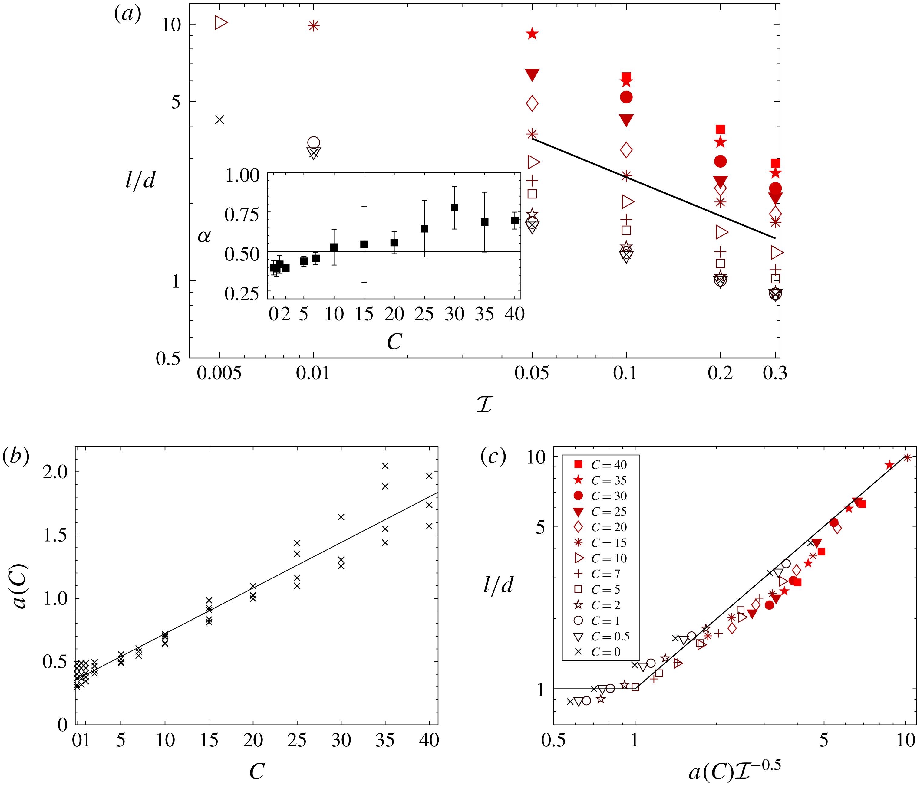
Figure 3(a) shows the velocity fluctuations measured in all flows at different inertial and cohesion numbers. The metric used is the dimensionless velocity fluctuation, which can be expressed in terms of a dimensionless length
 $\ell$
as:
 $$\begin{eqnarray}\frac{l}{d}=\frac{\unicode[STIX]{x1D6FF}v}{\dot{\unicode[STIX]{x1D6FE}}d}.\end{eqnarray}$$
Dependence of velocity fluctuations on inertial number and cohesion. (a) Non-dimensional velocity fluctuations (defined in (3.1)) measured in flows at different inertial and cohesion numbers; the solid line represents
 $l/d\propto {\mathcal{I}}^{-0.5}$
; symbols code is given in (c). Inset: Power-law coefficient in
 $l/d\propto {\mathcal{I}}^{-\unicode[STIX]{x1D6FC}}$
for each level of cohesion; error bars represent the standard error of the fit. (b) Parameter
 $a(C)$
obtained by fitting the measured velocity fluctuations in (a) by (3.2); the line represents the best linear fit of
 $a(C)$
, as per (3.3). (c) Comparison of the measured velocity fluctuations to the proposed model defined by (3.2) and (3.3); the line represents the function defined by
 $y=x$
for
 $x>1$
and
 $y=1$
otherwise.
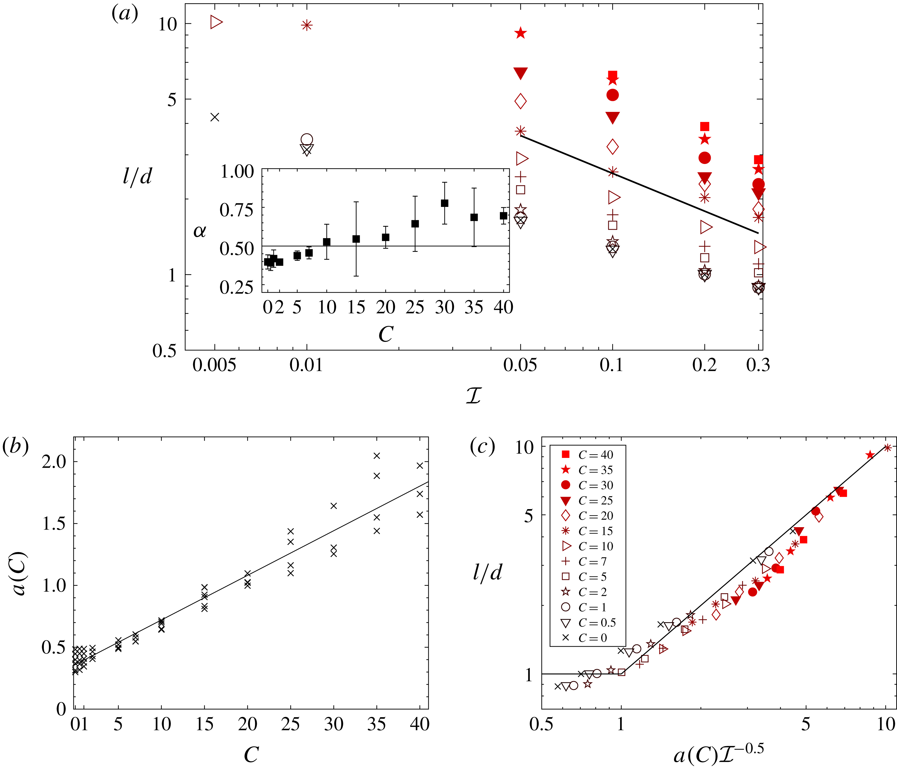
It appears that, for each level of cohesion, a power law governs inertial effects on this length:
 $l/d\sim {\mathcal{I}}^{-\unicode[STIX]{x1D6FC}}$
. Without cohesion, the power is approximately
 $\unicode[STIX]{x1D6FC}=0.5$
, which is consistent with results in DeGiuli et al. (Reference DeGiuli, McElwaine and Wyart2016) for this range of inertial number and interparticle friction. Best fits of the power
 $\unicode[STIX]{x1D6FC}$
shown on figure 3(a) inset evidence a slight increase with the level of cohesion. However, a constant value of
 $\unicode[STIX]{x1D6FC}(C)=0.5$
provides a reasonable approximation. Utilising this power constant, our data presented in figure 3(b,c) suggest that the velocity fluctuations in cohesive and cohesionless granular flows can be captured by the following empirical formulae:
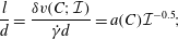 $$\begin{eqnarray}\displaystyle & \displaystyle \frac{l}{d}=\frac{\unicode[STIX]{x1D6FF}v(C;{\mathcal{I}})}{\dot{\unicode[STIX]{x1D6FE}}d}=a(C){\mathcal{I}}^{-0.5}; & \displaystyle\end{eqnarray}$$
 $$\begin{eqnarray}\displaystyle & \displaystyle a(C)\approx 0.35+0.04C. & \displaystyle\end{eqnarray}$$
Figure 3(c) shows that this formula captures the measured velocity fluctuations while
 $a(C){\mathcal{I}}^{-0.5}>1$
. For smaller values, the measured lever length reaches a minimum of
 $l=d$
.
The increasing nature of
 $a(C)$
indicates that cohesion produces larger velocity fluctuations for any given inertial number, which contributes to enhancing diffusion, as per the Green–Kubo formula. However, this does not explain the breakdown of the scaling (1.1) between diffusivity and velocity fluctuations that is observed at high cohesion (
 $C\gtrsim 8$
).
3.2 Memory time
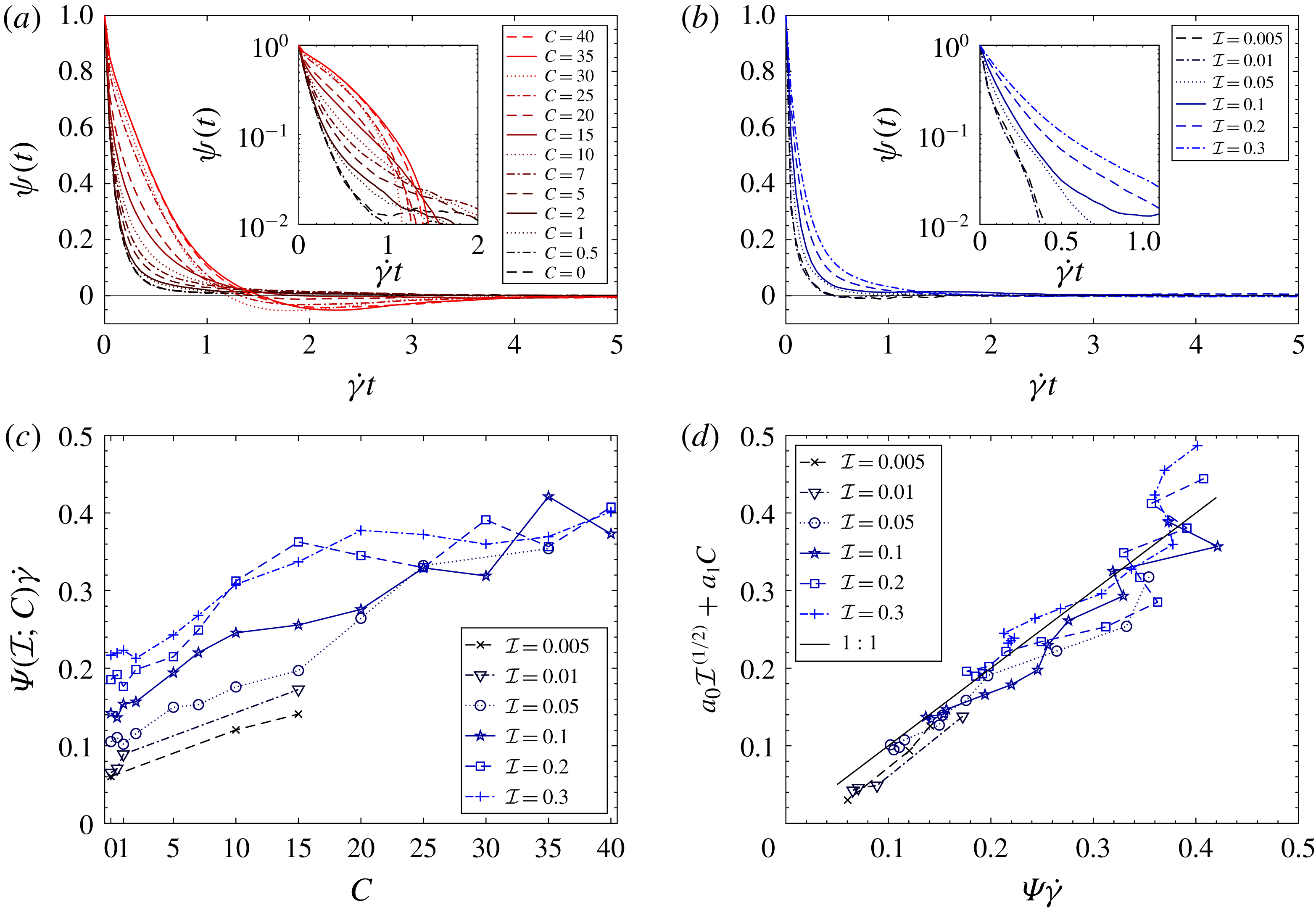
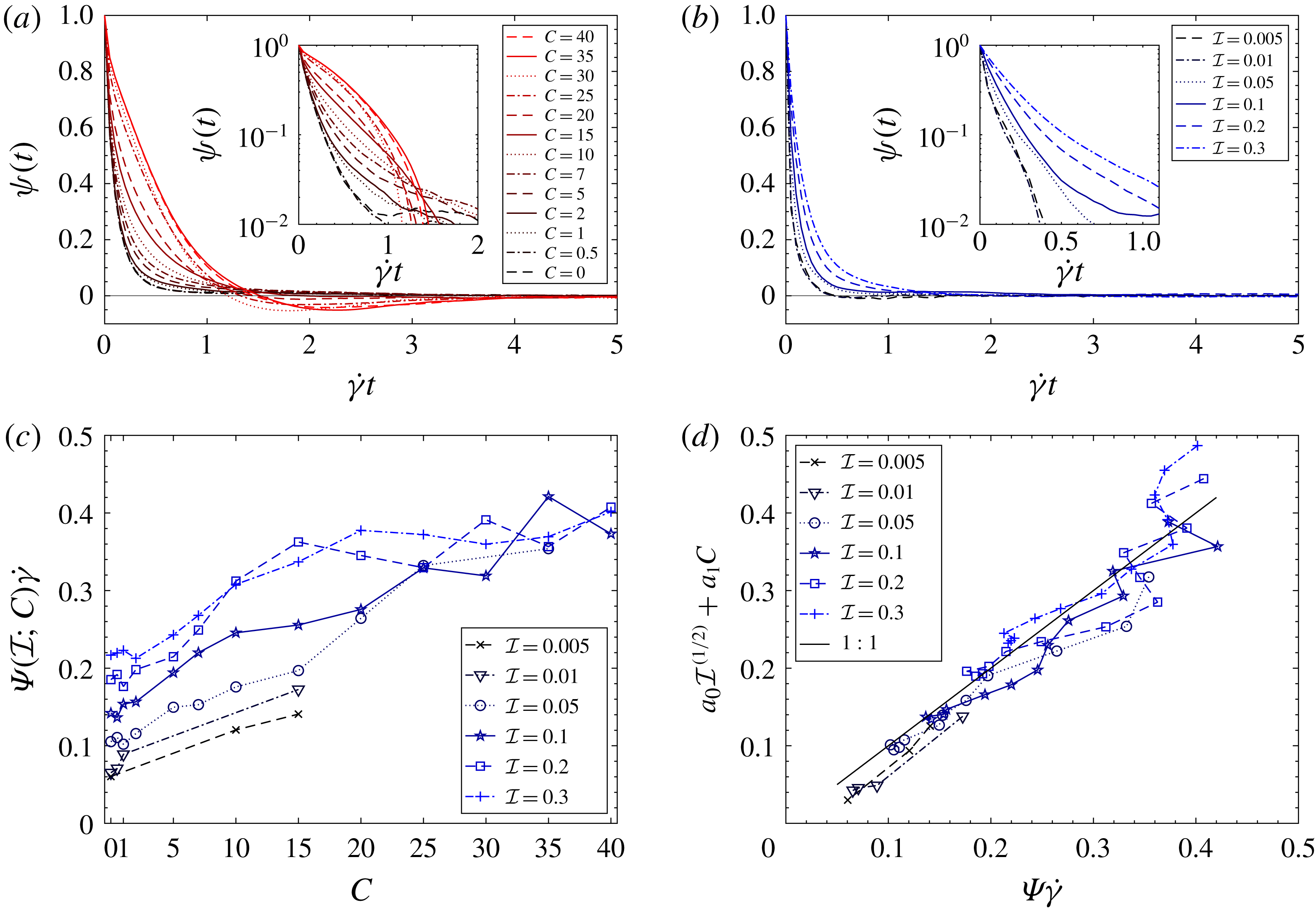
Figure 4(a,b) shows the velocity fluctuations correlation function
 $\unicode[STIX]{x1D713}(t)$
measured in cohesive and cohesionless flows. Without cohesion, this function drops towards zero in a time scale that is much smaller than the shear time
 $\dot{\unicode[STIX]{x1D6FE}}^{-1}$
. It never becomes negative. With cohesion, the initial decay of
 $\unicode[STIX]{x1D713}(t)$
is longer. At with high cohesion and inertial number, the correlation becomes negative, with a minimum reached at approximately
 $t\dot{\unicode[STIX]{x1D6FE}}=2$
, before converging towards zero. In a first approximation, the initial decay of the correlation function is seemingly exponential.
Figure 4(c) shows the corresponding normalised velocity fluctuation memory times
 $\unicode[STIX]{x1D6F9}\dot{\unicode[STIX]{x1D6FE}}$
, defined in (2.3). This memory time appears to increase both with
 ${\mathcal{I}}$
and
 $C$
, from minimum values of 0.06 up to maximum values of about 0.40. The negative velocity autocorrelation observed in figure 4(a) contributes to a plateau along
 ${\mathcal{I}}=0.3$
.
This is consistent with the existence of long-lived clusters which, thanks to cohesion, may persist for long period of times – possibly longer than a shear deformation
 $\dot{\unicode[STIX]{x1D6FE}}$
. As far as grain mixing is concerned, an optimal cluster persistence would be half a rotation. Clusters living longer will bring grains back closer to their initial position (Griffani et al.
Reference Griffani, Rognon, Metzger and Einav2013). This effect is evidenced in negative values of the velocity correlations observed in figure 4(a,b) at high cohesion.
We propose the following empirical scaling for the memory time, that accounts for an increase with cohesion:
 $$\begin{eqnarray}\unicode[STIX]{x1D6F9}\dot{\unicode[STIX]{x1D6FE}}\approx a_{0}{\mathcal{I}}^{1/2}+a_{1}C.\end{eqnarray}$$
Figure 4(d) compares the measured memory time to this model with
 $a_{0}=0.42\pm 0.02$
and
 $a_{1}=0.0064\pm 0.0004$
(standard errors), and evidences a reasonable match, with some deviations. We attribute this scattering to the finite size of the system and the finite duration of the simulations. This results in a limited number of large and long-lived clusters forming over the course of the simulation, and a statistical uncertainty associated with the ensemble average. We note that (3.4) predicts a divergence in
 $\unicode[STIX]{x1D6F9}$
when the shear rate tends to 0. This is consistent with stationary configurations having infinite memory time.
Memory time of velocity fluctuations. (a) Velocity autocorrelation function
 $\unicode[STIX]{x1D713}(t)$
for
 ${\mathcal{I}}=0.1$
with different
 $C$
. (b)
 $\unicode[STIX]{x1D713}(t)$
for
 $C=0$
with different
 ${\mathcal{I}}$
. Insets in (a,b) show semi-log plots of the initial decay of
 $\unicode[STIX]{x1D713}(t)$
. (c) Particle memory time (defined in (2.3)) for all plane shear flows with differing inertial and cohesion numbers. (d) Measured memory times compared to the empirical model in (3.4). The goodness of fit is
 $r^{2}=0.89$
.
3.3 Cluster-led random walks
We now seek to interpret the measured shear-induced diffusivity in terms of cluster length and persistence time. In this aim, we use Einstein’s framework that relates the diffusivity to an elementary random walk of step size
 $\ell _{r}$
and frequency
 $t_{r}^{-1}$
, as
 $D\propto \ell _{r}^{2}/t_{r}$
. The question is to establish how clusters affect these length and time scales.
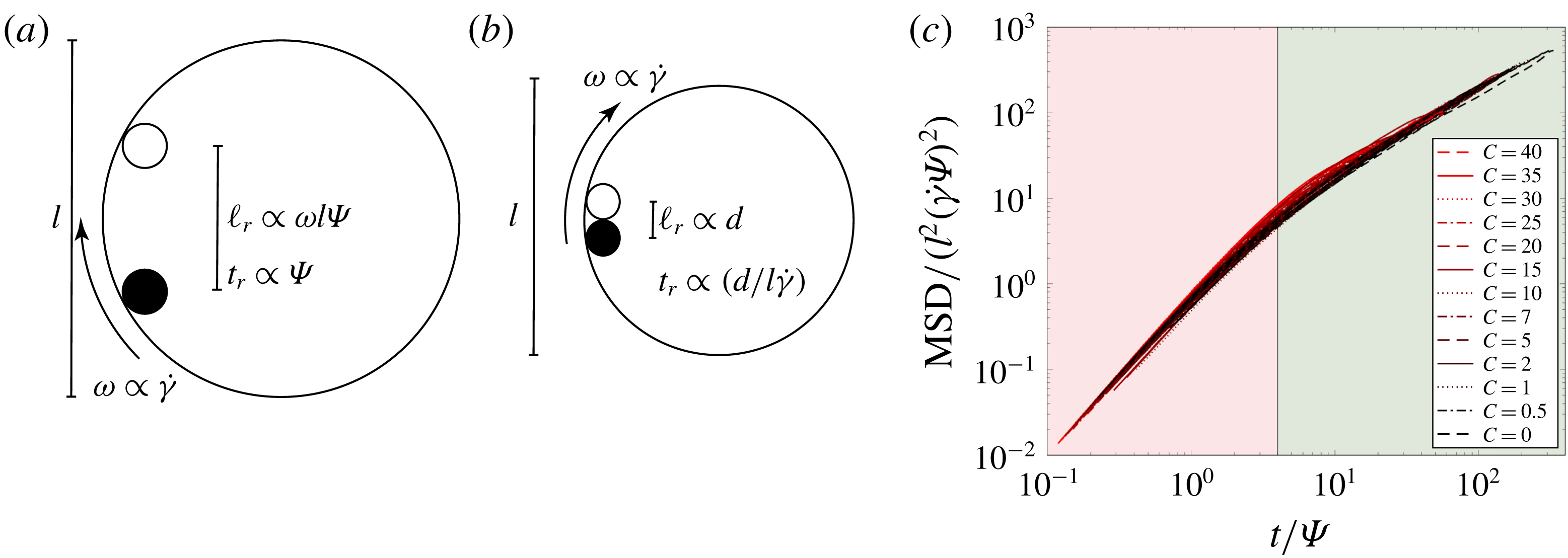
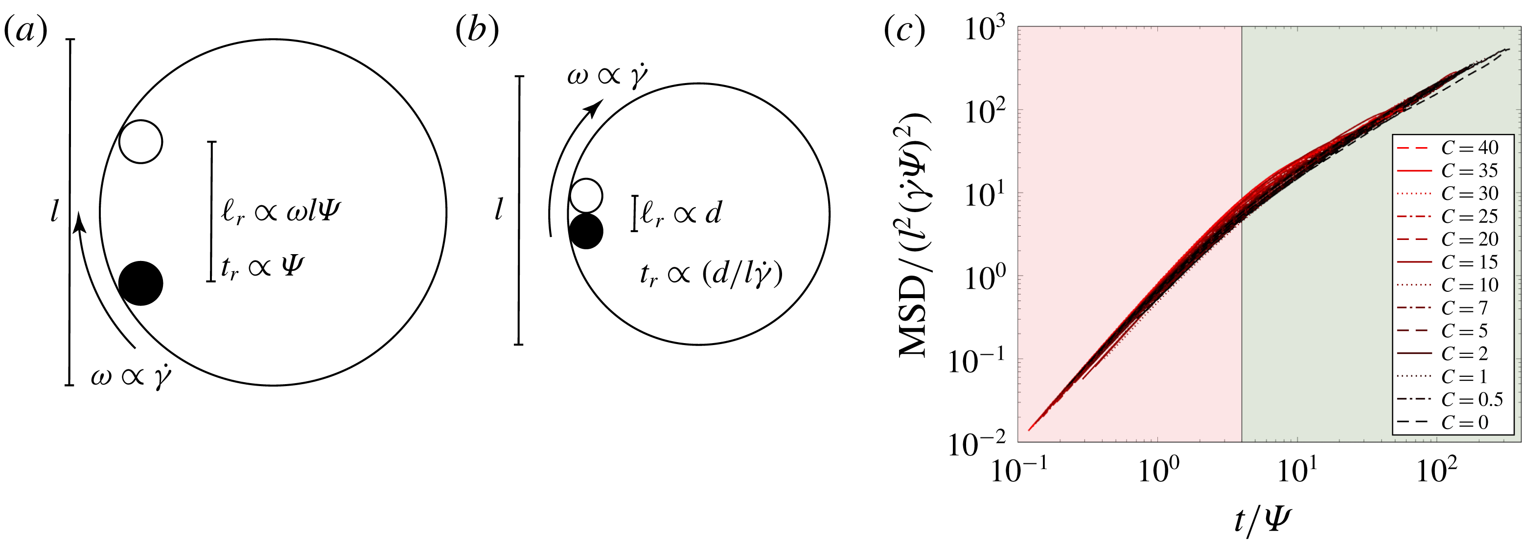
With cohesion (a), larger and more persistent clusters diffuse particles on longer distances (
 $\ell _{r}$
) with lower frequency (
 $t_{r}^{-1}$
) compared to smaller, short-lived, cohesionless clusters (b). (c) MSDs (same data as on figure 2
a) normalised by the effective cluster size, as a function of time normalised by the cluster persistence time
 $\unicode[STIX]{x1D6F9}$
(different
 ${\mathcal{I}}$
, different cohesion). Pink and green backgrounds indicate the superdiffusive and normal-diffusive regimes, respectively.
We consider rigid clusters of grains of size
 $l$
, rotation speed
 $\unicode[STIX]{x1D714}\propto \dot{\unicode[STIX]{x1D6FE}}$
, and persistence time
 $\unicode[STIX]{x1D6F9}$
, as depicted in figure 5(a). Over its lifetime, such a cluster would move the grains at its periphery by a step size
 $\ell _{r}\propto \unicode[STIX]{x1D714}l\unicode[STIX]{x1D6F9}$
or, more generally (such as for long-lasting clusters where
 $\unicode[STIX]{x1D6F9}>1/\dot{\unicode[STIX]{x1D6FE}}$
) some fixed step size
 $\ell _{r}(\unicode[STIX]{x1D714};l;\unicode[STIX]{x1D6F9})$
. Then, another cluster would form at a different and random location, moving again these grains in a different and random direction. This produces a random walk of step size
 $\ell _{r}\propto \unicode[STIX]{x1D714}l\unicode[STIX]{x1D6F9}$
and frequency
 $t_{r}^{-1}\propto \unicode[STIX]{x1D6F9}^{-1}$
. The resulting diffusivity of this cluster-led random walk is then expressed in terms of cluster size
 $l$
and lifetime
 $\unicode[STIX]{x1D6F9}$
as:
 $$\begin{eqnarray}D\propto \dot{\unicode[STIX]{x1D6FE}}^{2}l^{2}\unicode[STIX]{x1D6F9}.\end{eqnarray}$$
Under the current models for
 $l$
and
 $\unicode[STIX]{x1D6F9}$
, equation (3.5) reduces to the known cohesionless diffusion scaling in (1.3). This is done by utilising the length scale
 $l^{2}=d^{2}/{\mathcal{I}}$
from (1.2) and the cohesionless version of (3.4):
 $\unicode[STIX]{x1D6F9}\propto {\mathcal{I}}^{1/2}/\dot{\unicode[STIX]{x1D6FE}}$
. Figure 5(b) depicts the corresponding reduced random walk.
Figure 5(c) confirms the relevance of this process to granular shear-induced diffusivity. It shows a linear scaling between the MSDs rescaled by the cluster length
 $\ell _{r}^{2}=l^{2}(\dot{\unicode[STIX]{x1D6FE}}\unicode[STIX]{x1D6F9})^{2}$
with time rescaled by
 $\unicode[STIX]{x1D6F9}$
in the normal-diffusive regime, which indicates a diffusivity scaling similar to (3.5). Further still, this figure shows a full collapse of both the superdiffusive and normal-diffusive regimes. It demonstrates a diffusion regime transition happening after a period of time in the order of the cluster lifetime,
 $t\propto \unicode[STIX]{x1D6F9}$
, which produces a MSD scaling like
 $\ell _{r}^{2}$
. This is consistent with a cluster-induced advective motion of grains on a distance
 $\ell _{r}$
, as an elementary random step.
4 Conclusion
This study shows that cohesive forces can strongly affect shear-induced diffusion in dense granular flows. In the explored range of inertial and cohesion numbers, cohesion can increase the diffusivity by up to two orders of magnitude.
We attribute this increase to two drivers related to the existence of large and long-lived cohesive clusters: their size and their persistence time. Cohesion is found to increase both of these quantities. As a consequence, at high cohesion, the scalings (1.1)–(1.3) are no longer valid. Instead, we propose a general relationship between diffusivity and cluster size and lifetime (3.5), that is valid for both cohesive and cohesionless grains.
While this study focuses on homogeneous and bi-dimensional flows, we expect this relationship to be valid in heterogeneous and three-dimensional flows featuring clusters. However, the cluster size and life time in these configurations remain to be established. Nonetheless, our results suggest that similar shear-induced diffusion behaviours may be expected with other particulate fluids where flow structures underpin diffusive processes. These include foams, emulsions, suspensions and colloids in presence of cohesive forces. They also pave the way for further analysis of transport properties such as diffusion of momentum (or viscosity) in these materials.
Supplementary movies
Supplementary movies are available at https://doi.org/10.1017/jfm.2018.861.
Appendix A
The system contains
 $n=10^{4}$
cylinders with diameters randomly drawn from
 ${\mathcal{U}}(0.8d,1.2d)$
, corresponding to a mean grain diameter
 $d$
and mean grain mass
 $m$
. The top and bottom boundaries (
 $y=\pm L_{y}/2$
) move in the
 $x$
-direction according to the desired shear rate
 $\dot{\unicode[STIX]{x1D6FE}}$
so that walls maintain
 $v_{w}=\pm (L_{y}/2)\dot{\unicode[STIX]{x1D6FE}}$
. The system width
 $L_{x}=\sqrt{n}d=100d$
is fixed. The system’s vertical stress is subjected to a viscous boundary dynamic
 $\dot{L}_{y}=((\unicode[STIX]{x1D70E}/P)-1)d\dot{\unicode[STIX]{x1D6FE}}/20$
to maintain
 $\unicode[STIX]{x1D70E}\approx P$
.
Grains with an overlap
 $\unicode[STIX]{x1D6FF}_{ij}=d_{i}/2+d_{j}/2-|\unicode[STIX]{x0394}\boldsymbol{x}_{ij}|$
interact through elastic, frictional, dissipative, and cohesive contact forces. A Heaviside function
 $\unicode[STIX]{x1D6E9}(\unicode[STIX]{x1D6FF}_{ij})$
with magnitude
 $f_{0}$
governs the cohesive normal forces between particles. Many contact models exist for cohesion; however, provided that they have an identical maximum cohesive force
 $\max (f_{0})$
, comparisons between various capillary force models show negligible difference in macroscopic flow behaviours (Richefeu et al.
Reference Richefeu, El Youssoufi, Peyroux and Bohatier2005; Rognon et al.
Reference Rognon, Roux, Wolf, Naaïm and Chevoir2006; Luding Reference Luding2008).
An elastic modulus
 $E=1000P$
dictates the elastic repulsive force
 $F_{El}=Ed\unicode[STIX]{x1D6FF}_{ij}$
. The viscous normal force is
 $F_{Vis}=\unicode[STIX]{x1D702}dV_{ij}$
, with fixed viscosity
 $\unicode[STIX]{x1D702}$
and where
 $dV_{ij}$
is the intergranular velocity differential. The tangential frictional force between grains is
 $F_{T}=\min (Ed\dot{u}\unicode[STIX]{x0394}t,\unicode[STIX]{x1D707}_{p}F_{El})$
, where
 $\dot{u}$
is the relative tangential velocity at the point of contact and
 $\unicode[STIX]{x1D707}_{p}=0.5$
is the interparticle friction. In total, the contact force is given by:
 $$\begin{eqnarray}\boldsymbol{F}_{ij}=\hat{\boldsymbol{n}}_{ij}^{N}(F_{El}+F_{Vis}+f_{0})+\hat{\boldsymbol{n}}_{ij}^{\text{T}}(F_{T}).\end{eqnarray}$$
The characteristic elastic collision time sets the simulation time step at
 $\unicode[STIX]{x0394}t=(1/20)\sqrt{m/Ed}$
.
Steady flow regimes are identified by checking that a constant volume fraction and a constant stress tensor mean is reached. Spatial shear homogeneity in this regime is assessed using a method introduced in Khamseh et al. (Reference Khamseh, Roux and Chevoir2015) and DeGiuli et al. (Reference DeGiuli, McElwaine and Wyart2016). The method consists of detecting stationary shear bands by measuring by how much the time-averaged velocity profiles
 $\bar{v}(y)$
deviates from a linear profile, using the quantity:
 $\unicode[STIX]{x1D6E5}=(12/\dot{\unicode[STIX]{x1D6FE}}^{2}H^{2})1/H\int _{-H/2}^{H/2}(\bar{v}(y)-\dot{\unicode[STIX]{x1D6FE}}y)^{2}\,\text{d}y$
.
 $\unicode[STIX]{x1D6E5}=1$
corresponds to a pure shear band and
 $\unicode[STIX]{x1D6E5}=0$
to a homogeneous shear. We consider flows to be homogeneous when
 $\unicode[STIX]{x1D6E5}<0.25$
.
Appendix B
Mean square displacements are computed over a range of starting times
 $t_{0}^{k}\in [0,t_{Max}]$
with
 $k\in [1,N]$
provided that
 $\unicode[STIX]{x1D70F}+t_{0}^{k}\leqslant t_{Max}$
. Lags are spaced every
 $\unicode[STIX]{x0394}\unicode[STIX]{x1D70F}=20/\dot{\unicode[STIX]{x1D6FE}}$
.
 $$\begin{eqnarray}\langle \unicode[STIX]{x0394}y^{2}(\unicode[STIX]{x1D70F})\rangle =\langle [y_{g}(\unicode[STIX]{x1D70F})-y_{g}(0)]^{2}\rangle =\frac{1}{n(N-k)}\mathop{\sum }_{g=1}^{n}\mathop{\sum }_{k=1}^{N-k}[y_{g}(t_{0}^{k}+\unicode[STIX]{x1D70F})-y_{g}(t_{0}^{k})]^{2}.\end{eqnarray}$$
Monitoring of grains passing over the boundaries allows recording of non-periodic (Euclidean) transverse displacements. Long-term normal diffusion coefficients are extracted using (2.2) for
 $5\leqslant \unicode[STIX]{x1D70F}\dot{\unicode[STIX]{x1D6FE}}\leqslant 20$
, provided the goodness of fit exceeded
 $r^{2}>0.98$
.
Appendix C
The normalised velocity autocorrelation in the transverse direction was computed for a range of delays
 $\unicode[STIX]{x1D70F}\in [0,t_{Max})$
. The ensemble average accounted for every grain and a range starting times
 $t_{0}^{k}\in [0,t_{Max}]$
using:
 $$\begin{eqnarray}\unicode[STIX]{x1D713}(\unicode[STIX]{x1D70F})=\frac{\langle v(0)\cdot v(\unicode[STIX]{x1D70F})\rangle }{\langle v(0)\cdot v(0)\rangle }=\frac{1}{n}\mathop{\sum }_{g=1}^{n}\frac{\displaystyle \mathop{\sum }_{k=1}^{N}[v_{g}(t_{0}^{k})\cdot v_{g}(t_{0}^{k}+\unicode[STIX]{x1D70F})]}{\displaystyle \mathop{\sum }_{k=1}^{N}[v_{g}(t_{0}^{k})\cdot v_{g}(t_{0}^{k})]};\end{eqnarray}$$
where
 $v_{g}(t)$
is the instantaneous transverse velocity (fluctuation) of grain
 $g$
at time
 $t$
with system drift removed (
 $\sum _{g=1}^{n}v_{g}$
). For numerical efficiency the autocorrelation was computed using the discrete Fourier transform
 ${\mathcal{F}}$
via the Wiener–Khinchin theorem
 $\sum _{k=1}^{N}[v_{g}(t_{0}^{k})\cdot v_{g}(t_{0}^{k}+\unicode[STIX]{x1D70F})]={\mathcal{F}}^{-1}[|{\mathcal{F}}(v_{g})|^{2}](\unicode[STIX]{x1D70F})$
.