



1. Introduction
The coupon collector’s problem (CCP) has a long history, dating back to de Moivre, Laplace, and Euler; see, for example, Sections 291, 448–461, 632–638, 775–781, 864, 910, and 971 of [Reference Todhunter37] for a detailed exposition of the early history of the CCP. The CCP has many applications (see, e.g., [Reference Boneh and Hofri8]), and it is of ongoing interest, as witnessed by the recent papers [Reference Aki and Hirano1–Reference Angus4, Reference Berenbrink, Sauerwald, Ngo and Springer6,Reference Berenbrink, Elsässer, Friedetzky, Nagel, Sauerwald, Murlak, Sankowski and Springer7, Reference Brown and Ross9–Reference Doumas and Papanicolaou13, Reference Falgas-Ravry, Larsson and Markström15–Reference Glavaš and Mladenović18, Reference Ilienko20–Reference May27, Reference Neal29–Reference Ross and Wu32, Reference Shank and Yang34, Reference Smythe35, Reference Xu and Tang38].
In the classical CCP there are n distinct types of coupon, and coupons are collected one at a time, independently of each other, with each type being equally probable. In this setting, let
 $W_{n,c}$
denote the number of coupons that must be sampled until each type has been sampled at least c times, where
 $c \ge 1$
is a fixed number.
In what follows we will adopt a conceptually equivalent interpretation, inasmuch as the n types of coupons represent n different cells, which are numbered from 1 to n, and the sampling of a type of coupon corresponds to the placement of a particle into a cell. In this setting, Erdös and Rényi [Reference Erdös and Rényi14] showed that, for each
 $x \in \mathbb{R}$
,
 \begin{equation}\lim_{n \to \infty} \mathbb{P} \left( W_{n,c} \le n \big{\{} \log n \! + \! (c\! -\! 1) \log \log n \! - \! \log(c\! -\! 1)! \! + \! x\big{\}} \right) = \exp\left(-\textrm{e}^{-x}\right).\end{equation}
In other words,
 $W_{n,c}/n - \log n - (c - 1) \log \log n + \log(c - 1)!$
has a Gumbel limit distribution as
 $n \to \infty$
.
This paper deals with the CCP with group drawings, which means that at each stage of the ‘placement process’, s particles are placed into s different cells, which is henceforth called an s-placement. A standard application is the collection of pictures of soccer players, where you can buy packages with
 $s=5$
or
 $s=6$
different pictures out of a total of several hundred pictures. The classical assumption in this more general setting is that each of the
 $\left(\begin{array}{c}n \\[-5pt] s \end{array}\right)$
s-placements, which are subsets of size s out of the n cells, has the same probability. In what follows, the random variable of interest is
 $W_{n,s,c}$
, which is the number of s-placements necessary to have at least c particles in each cell. In other words,
 $W_{n,s,c}$
is the waiting time to see each type of coupon at least c times. Under this assumption, [Reference Stadje36], among other things, derived the probability distribution of
 $W_{n,s,1}$
.
Suppressing the dependence on c, s, and k, define, for each
 $k \ge 1$
and
 $j \in \{1,\ldots,n\}$
,
 $A_{n,j}$
to be the event that, after k s-placements, cell j contains at most
 $c-1$
particles, and let
 \begin{eqnarray}Z_{n,s,c}(k) \;:\!=\; \sum_{j=1}^n {\bf 1}\{A_{n,j}\}\end{eqnarray}
denote the number of cells that contain at most
 $c-1$
particles after k s-placements, where
 ${\bf 1}\{ \cdot \}$
denotes the indicator function.
For fixed
 $x \in \mathbb{R}$
, let
 \begin{equation}k_{n,s,c}(x) = \Big{\lfloor} \frac{n}{s}\left(\log n+(c-1)\log\log n-\log(c-1)!+x \right) \Big{\rfloor}, \qquad n > 1,\end{equation}
where
 $\lfloor \cdot \rfloor$
denotes the floor function. In the special case
 $c=1$
, [Reference Mikhailov28, Theorem 2] yields
 \begin{equation}Z_{n,s,1}(k_{n,s,1}(x)) \stackrel{ \mathcal{ D}}{\longrightarrow} \textrm{Po}(\textrm{e}^{-x}), \qquad x \in \mathbb{R},\end{equation}
where
 $\stackrel{\mbox{D}}{\longrightarrow}$
denotes convergence in distribution, and
 $\textrm{Po}(\lambda)$
,
 $\lambda >0$
, is the Poisson distribution with parameter
 $\lambda$
. Notice that this result gives (1) in the special case
 $c=1$
, since
 $Z_{n,s,1}(k_{n,s,1}(x))=0$
if, and only if,
 $W_{n,1} \le n(x+ \log n)$
.
In this paper we first generalize (4) to the case
 $c>1$
in Section 2. In Section 3, we consider the special case
 $c=1$
, but relax the condition of a uniform distribution over all s-placements and consider, as
 $n \to \infty$
, a sequence of distributions over all s-placements that approach the uniform distribution at the rate
 $O(1/\log n)$
. For the sake of readability, parts of the proofs are deferred to Section 4.
2. A Poisson limit for the number of cells having at most
 $c-1$
particles

In this section we generalize (4) to the case
 $c>1$
and (1) to the case
 $s>1$
. Our main result is as follows.
Theorem 1. Under the condition that each s-placement is equally probable, we have
 $Z_{n,s,c}(k_{n,s,c}(x)) \stackrel{\mbox{D}}{\longrightarrow} Z$
as
 $n \to \infty$
,
 $x \in \mathbb{R}$
, where
 $k_{n,s,c}(x)$
is defined in (3), and Z has the Poisson distribution
 $\textrm{Po}(\textrm{e}^{-x})$
.
Since
 $W_{n,s,c} \le k_{n,s,c}(x)$
if and only if
 $Z_{n,s,c}(k_{n,s,c}(x)) =0$
, Theorem 1 yields the following corollary.
Corollary 1. For each
 $x \in \mathbb{R}$
, we have
 \begin{equation*}\lim_{n\to \infty} \mathbb{P}\left(W_{n,s,c} \le \frac{n}{s}\Big{\{} \log n + (c-1)\log \log n - \log (c-1)! + x \Big{\}} \right) = \exp\left(-\textrm{e}^{-x}\right).\end{equation*}
Notice that Corollary 1 indeed generalizes both (1) and (4). We mention that (1) may also be obtained from [Reference Ilienko20] (see Remark 4.3 there).
2.1. Proof of Theorem 1
Put
 $k_n = k_{n,s,c}(x)$
, and assume n to be sufficiently large in order to have
 $k_n \ge 1$
. For
 $\ell \in \{0,\ldots,c-1\}$
, let
 $A_{n,j}^{(\ell)}$
be the event that cell j contains
 $\ell$
particles after
 $k_n$
s-placements, and define
 $Z_{n,s,c}^{(\ell)}(k_n)\;:\!=\;\sum_{\ell=0}^{c-1}{\bf 1}\{A_{n,j}^{(\ell)}\}$
. Then,
 $Z_{n,s,c}(k)$
figuring in (2), with k replaced with
 $k_n$
, takes the form
 $Z_{n,s,c}(k_n)=\sum_{\ell=0}^{c-1}Z_{n,s,c}^{(\ell)}(k_n)$
. By the definition of
 $k_n$
, straightforward calculations yield
 \begin{equation*}\mathbb{E} Z_{n,s,c}^{(\ell)}(k_n) = n\mathbb{P}\big(A_{n,1}^{(\ell )}\big) = n \binom{k_n}{\ell} \left(\frac{s}{n}\right)^\ell \left(1- \frac{s}{n}\right)^{k_n-\ell} = O\left((\log n)^{\ell-(c-1)}\right).\end{equation*}
Invoking Markov’s inequality, we have
 $Z_{n,s,c}^{(\ell)}(k)\stackrel{\mbox{P}}{\longrightarrow} 0$
as
 $n \to \infty$
if
 $\ell \le c-2$
. Thus, putting
 $Z_n \;:\!=\; Z_{n,s,c}^{(c-1)}(k_{n,s,c}(x))$
, it remains to prove that
 $Z_n \stackrel{\mbox{D}}{\longrightarrow} Z$
as
 $n \to \infty$
.
The proof uses the method of moments. The distribution of Z is uniquely determined by the sequence
 $({\mathbb{E}}(Z^r))_{r\ge 1}$
, and we have
 ${\mathbb{E}}(Z^r) = \sum_{\ell =0}^r \big{\{} \substack{r \\ i} \big{\}} {\mathbb{E}}( Z^{\underline{i }})$
, where, in a general notation,
 $t^{\underline{i}}= t(t-1)\cdots (t-i+1)$
denotes the ith descending factorial of
 $t \in \mathbb{R}$
, and
 $\big{\{} \substack{r \\ i} \big{\}} $
,
 $i =0,\ldots,r$
, are the Stirling numbers of the second kind (see [Reference Graham, Knuth and Patashnik19, p. 262]). Since
 ${\mathbb{E}}(Z^{\underline{r}}) = \lambda^r$
, where
 $\lambda = \textrm{e}^{-x}$
, and since the events
 $A_{n,j}^{(c-1)}$
,
 $1 \le j \le n$
, are exchangeable, we have
 $ {\mathbb{E}}(Z_n^{\underline{r}}) = n^{\underline{r}} \, {\mathbb{P}}\big(A^{(c-1)}_{n,1}\cap \cdots \cap A^{(c-1)}_{n,r}\big)$
. In view of
 $n^{\underline{r}}/n^r \to 1$
as
 $n \to \infty$
, it thus remains to prove that
 \begin{equation}\lim_{n\to \infty} n^r \, {\mathbb{P}}\Big(A^{(c-1)}_{n,1}\cap \cdots \cap A^{(c-1)}_{n,r}\Big) = \lambda^r\end{equation}
for each
 $r \ge 1$
. To this end, let
 $N_{n,j}$
be the number of particles in cell j after
 $k_n$
s-placements, whence
 \begin{equation}{\mathbb{P}}\big(A_{n,1}^{(c-1)}\cap \cdots \cap A^{(c-1)}_{n,r}\big) = {\mathbb{P}}(N_{n,1} = c-1,\ldots, N_{n,r} = c-1).\end{equation}
Notice that if
 $r \ge 2$
, more than one of the cells
 $1,\ldots,r$
may receive a particle in each s-placement. We will see, however, that this event will be asymptotically negligible. For this purpose, let
 $B_i$
denote the number of all
 $k_n$
s-placements in which exactly i of the cells
 $1,\ldots,r$
receive a particle, where
 $i \in \{1,\ldots,r\}$
, and put
 $B\;:\!=\; (B_1,\ldots,B_r)$
. Setting
 $N_j \;:\!=\; N_{n,j}$
and
 $b\;:\!=\;(b_1,\ldots,b_r)$
, we then have
 \begin{align} {\mathbb{P}}(N_1 &= c-1,\ldots, N_r = c-1)\nonumber \\ & = \sum_{b_1 \ge 0} \cdots \sum_{b_r \ge 0} {\mathbb{P}}(N_1 = c-1,\ldots,N_r = c-1,B = b) {\bf 1} \left\{\sum_{j=1}^r jb_j = r(c-1)\right\}. \end{align}
Notice that, under the condition
 $s<r$
,
 ${\mathbb{P}}(N_1 = c-1,\ldots,N_r = c-1,B = b)$
can only be positive if
 $b_{s+1}= \cdots = b_r=0$
. The abovementioned asymptotic negligibility is a consequence of the following result, the proof of which is given in Section 4.
Lemma 1.
 ${\mathbb{P}}(N_1 = c-1,\ldots,N_r = c-1,B = b) = \displaystyle{O\big({n^{-r-\sum_{i=2}^r (i-1)b_i}}\big) }$
.
We now put
 ${\mathcal{S}}_{n,r,s} \;:\!=\; \mathbb{P}\left(N_{1}=c-1,\ldots ,N_{r}=c-1,B_1=r(c-1),B_2=\cdots =B_r=0\right)$
. In view of (5)–(7) and Lemma 1, we obviously have to show that
 \begin{equation}\lim_{n \to \infty} n^r {\mathcal{S}}_{n,r,s} =\lambda^r.\end{equation}
Similar to the reasoning given in the proof of Lemma 1, it follows that
 \begin{equation*} {\mathcal{S}}_{n,r,s} =\dfrac{k_n!}{(c-1)!^r (k_n-r(c-1))!} \left[\frac{\binom{n-r}{s-1}}{\binom{n}{s}}\right]^{r(c-1)} \left[\frac{\binom{n-r}{s}}{\binom{n}{s}}\right]^{k_n-r(c-1)}.\end{equation*}
Now,
 $k_n!/(k_n-r(c-1))! = k_n^{r(c-1)}(1+o(1))$
and
 $\binom{n -r}{s-1}/\binom{n}{s} = (s/n)(1+o(1))$
. Moreover,
 \begin{equation*}\frac{\binom{n-r}{s}}{\binom{n}{s}}=\prod_{i=0}^{r-1}\left(1-\frac{s}{n-i}\right),\end{equation*}
and we obtain
 \begin{equation*} {\mathcal{S}}_{n,r,s} = \left(\frac{k_n s}{n}\right)^{r(c-1)} \left[\prod_{i=0}^{r-1} \left(1-\frac{s}{n-i}\right)\right]^{k_n-r(c-1)} \frac{(1+o(1))}{(c-1)!^r}.\end{equation*}
We now take the logarithm of
 ${\mathcal{S}}_{n,r,s}$
. By the definition of
 $k_n$
, straightforward calculations yield
 \begin{equation*}r(c-1)\log\left( \frac{k_n s}{n}\right) = r(c-1) \log \log n +o(1).\end{equation*}
Since
 $\log t \le t-1$
,
 $t >0$
, we further have
 \begin{eqnarray} (k_n \! - \! r(c-1)) \textstyle{\sum_{i=0}^{r-1}\log\left(1 \! - \! \frac{s}{n-i}\right)} & \le & -(k_n - r(c-1)) \textstyle{\sum_{i=0}^{r-1}\frac{s}{n-i}}\\ & \le & -(k_n - r(c-1))\cdot \frac{rs}{n} \nonumber\\ & = & -rx-r\log n-r(c-1)\log\log n+r\log(c-1)! + o(1).\nonumber \end{eqnarray}
Upon exponentiating, it thus follows that
 \begin{equation*} n^r {\mathcal{S}}_{n,r,s} \le \textrm{e}^{-rx+o(1)}(c-1)!^r \exp\left[(\log\log n)\left(r(c-1)-r(c-1)\right)\right]\frac{1}{(c-1)!^r}.\end{equation*}
We obtain
 \begin{equation}\limsup_{n \to \infty} n^r {\mathcal{S}}_{n,r,s} \le \textrm{e}^{-rx} = \lambda^r.\end{equation}
In the same way, using the inequality
 $\log t \ge 1-1/t$
,
 $t >0$
, to bound the left-hand side of (9) from below, it follows that
 $\liminf_{n \to \infty} n^r {\mathcal{S}}_{n,r,s} \ge \textrm{e}^{-rx} = \lambda^r$
. The details are omitted. Together with (10), (8) follows, and the proof is completed.
3. A Poisson limit in the case
$\textbf{{c}}\;\textbf{=1}$
and nonuniform distributions

In this section we consider the waiting time until each cell has received at least one particle, but allow for small deviations from the uniform distribution over all subsets of size s of the n cells. For the special case
 $s=1$
, this case has been treated by [Reference Neal29]. To have a somewhat more compact notation, we put
 $[n]\;:\!=\; \{1,\ldots, n\}$
and let
 $[n]_s$
denote the system of all subsets of size s of [n]. For
 $\mathcal{I} \in [n]_s$
, we write
 $p_{n,\mathcal{I}}$
for the probability that each of the cells
 $i \in \mathcal{I}$
receives a particle in an s-placement. Our model is
 \begin{equation}p_{n,\mathcal{I}} = \dfrac{1}{\binom{n}{s}}\left(1+\dfrac{\Delta_{n,\mathcal{I}}}{\log n}\right),\end{equation}
where
 $\sum_{\mathcal{I} \in [n]_s} \Delta_{n,\mathcal{I}} =0$
and
 \begin{equation}\max_{\mathcal{I} \in [n]_s}|\Delta_{n,\mathcal{I}}| \le M\end{equation}
for some universal constant
 $M\in (0,\infty)$
. Thus, the deviation from a uniform distribution over
 $[n]_s$
is of order
 $1/\log n$
. To state the main theorem of this section, let, for
 $h \in \{1,\ldots,s\}$
and
 $\{i_1,\ldots,i_h\}\subset [n]$
,
 \begin{equation}\overline{\Delta}_{n,i_1,\ldots,i_h} \;:\!=\; \frac{1}{\binom{n-h}{s-h}} \sum_{\mathcal{I}\subset [n]_s: \mathcal{I}\supset \{i_1,\ldots,i_h\}} \Delta_{n,\mathcal{I}}\end{equation}
denote the average deviation from the uniform distribution over all s-placements
 $\mathcal{I}$
that occupy the cells
 $i_1,\ldots,i_h$
. Notice that
 $\Delta_{n,\mathcal{I}} = \overline{\Delta}_{n,i_1,\ldots,i_h}$
if
 $s=h$
. With
 $Z_{n,s,c}$
defined in (2) and
 $k_{n,s,c}(x)$
given in (3), we have the following result.
Theorem 2. Under the assumptions made above and the condition
 \begin{equation}\lim_{n\to \infty} \frac{1}{n} \sum_{i=1}^{n}\exp\left(-\frac{x+\log n}{\log n}\cdot \overline{\Delta}_{n,i} \right)=:c(x)
< \infty\text{, }\end{equation}
 $Z_{n,s,1}(k_{n,s,1}(x)) \stackrel{\mbox{D}}{\longrightarrow} Z$
as
 $n \to \infty$
,
 $x \in \mathbb{R}$
, where Z has the Poisson distribution
 $\textrm{Po}(\lambda)$
,
 $\lambda = \textrm{e}^{-x}c(x)$
.
Corollary 2. For the waiting time
 $W_{n,s,1}$
until each cell contains at least one particle we have, under the model (11),
 \begin{equation}\lim_{n\to\infty}\mathbb{P}\left( W_{n,s,1} \le \frac{n}{s}\big{\{} x + \log n\big{\}} \right) = G\left(x-\log c(x)\right)\text{,}\end{equation}
where
 $G(x) = \exp(-\textrm{e}^{-x})$
is the distribution function of the Gumbel distribution.
Before we give a proof of Theorem 2, we present two examples for the model (11).
Example 1. Suppose that the set [n] of cells is divided into
 $\ell$
pairwise disjoint blocks
 $B_{n,1}, \ldots, B_{n,\ell}$
, such that
 $[n] = B_{n,1}\cup \cdots \cup B_{n,\ell}$
and
 $\rho_{n,j} \;:\!=\; |B_{n,j}| \ge s$
,
 $j=1,\ldots,\ell$
, where
 $|B|$
denotes the number of elements of a finite set B. Without loss of generality we let
 $B_{n,1} = \{1,\ldots,\rho_{n,1}\}$
,
 $B_{n,2}= \{\rho_{n,1}+1,\ldots,\rho_{n,1}+\rho_{n,2}\}$
, etc.
We assume that the proportions of the blocks stabilize as
 $n \to \infty$
, i.e. we have
 \begin{equation}\lim_{n\to \infty} \frac{\rho_{n,j}}{n} = p_j, \qquad j=1,\ldots,\ell ,\end{equation}
(say), where
 $p_j>0$
for each j and
 $p_1+ \cdots + p_\ell =1$
. Furthermore, let
 $w_n\;:\!=\;(w_{n,1},\ldots,w_{n,\ell})$
be a sequence of ‘weight vectors’ in
 $\mathbb{R}^\ell$
such that
 $w_n \to w\;:\!=\;(w_1,\ldots,w_\ell)$
as
 $n \to \infty$
. We assume that
 \begin{equation}\sum_{j=1}^\ell \rho_{n,j} w_{n,j} =0\end{equation}
for each n, which implies
 $\sum_{j=1}^\ell p_jw_j =0$
. In other words, the vectors
 $p=(p_1,\ldots,p_\ell)$
and w are orthogonal. For
 $\mathcal{I} \in [n]_s$
, let
 $\Delta_{n,\mathcal{I}} \;:\!=\; \sum_{j=1}^\ell w_{n,j} |\mathcal{I}\cap B_{n,j}|$
. Notice that, in view of
 \begin{equation*}\sum_{\mathcal{I}\in [n]_s} \Delta_{n,\mathcal{I}} = \sum_{j=1}^{\ell}w_{n,j} \sum_{\mathcal{I}\in [n]_s}|\mathcal{I}\cap B_{n,j}| = \sum_{j=1}^{\ell}w_{n,j}\binom{n-1}{s-1} \rho_{n,j}\end{equation*}
and (17), we have
 $\sum_{\mathcal{I} \in [n]_s} \Delta_{n,\mathcal{I}} =0$
. To determine c(x) figuring in (14), notice that, by symmetry,
 $\overline{\Delta}_{n,i}$
is constant over i within each of the blocks, and hence the left-hand side of (14) (without the limit) takes the form
 \begin{equation*}\sum_{j=1}^\ell \frac{\rho_{n,j}}{n} \exp\left(-\frac{x+\log n}{\log n}\cdot \overline{\Delta}_{n,j_1} \right),\end{equation*}
where
 $j_1$
denotes the first element of block
 $B_{n,j}$
. Without loss of generality we choose the first block and notice that
 \begin{equation*}\overline{\Delta}_{n,1} = \dfrac{1}{\binom{n-1}{s-1}}\sum_{k=1}^{\ell}w_{n,k}\sum_{\mathcal{I}\in [n]_s: \mathcal{I}\ni 1}|\mathcal{I}\cap B_{n,k}|.\end{equation*}
We now consider the cases
 $k=1$
and
 $k>1$
separately. If we distinguish cases according to
 $m \;:\!=\; |\mathcal{I}\cap B_{n,1}|$
, it follows that
 \begin{equation*}\sum_{\mathcal{I}\in [n]_s: \mathcal{I}\ni 1}|\mathcal{I}\cap B_{n,1}| = \sum_{m =1}^s m \binom{\rho_{n,1}-1}{m -1} \binom{n-\rho_{n,1}}{s-m}= \binom{n-1}{s-1}\left( 1 + (s-1)\frac{\rho_{n,1}}{n}\right).\end{equation*}
Likewise, if
 $k>1$
we have
 \begin{equation*}\sum_{\mathcal{I}\in [n]_s: \mathcal{I}\ni 1}|\mathcal{I}\cap B_{n,k}| = \sum_{i =0}^{s-1} i \binom{\rho_{n,k}}{i} \binom{n-\rho_{n,k}-1}{s-i-1} =\binom{n-1}{s-1} \frac{(s-1)\rho_{n,k}}{n-1}.\end{equation*}
Summarizing, it follows that
 \begin{equation*}\overline{\Delta}_{n,1} = w_{n,1}\left(1+ \frac{(s-1)\rho_{n,1}}{n}\right) + \sum_{k=2}^\ell w_{n,k} \frac{(s-1)\rho_{n,k}}{n}\end{equation*}
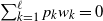
and thus, in view of (16),
 $w_{n,j} \to w_j$
, and
 $\sum_{k=1}^\ell p_kw_k=0$
, we deduce that
 $\lim_{n\to \infty} \overline{\Delta}_{n,1} = w_1$
. Since
 $(x+\log n)/\log n \to 1$
as
 $n \to \infty$
, we obtain
 $c(x) = \sum_{j=1}^\ell p_j \textrm{e}^{-w_j}$
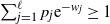
, independently of x. Notice that
 $\sum_{j=1}^\ell p_j \textrm{e}^{-w_j} \ge 1$
, and thus
 $\log c(x) \ge 0$
. This means that, at least under the sequence of alternative distributions to uniformity studied in this example, the limit distribution of
 $W_{n,s,1}$
is stochastically greater than under the assumption of a uniform distribution of all subsets of size s of [n].
Example 2. In the special case
 $s=1$
, a natural class of examples for the deviation (11) from the uniform distribution is given by
 \begin{equation*}p_{n,j} \;:\!=\; p_{n,\{j\}} = \frac{1}{n} \left( 1+ \frac{1}{\log n} \cdot n \int_{(j-1)/n}^{j/n} m(t) \, \textrm{d}t\right),\end{equation*}
where
 $m \colon [0,1] \rightarrow \mathbb{R}$
is a continuous function satisfying
 $\int_0^1 m(t) \, \textrm{d}t=0$
. Here, by the mean value theorem, we have
 $\Delta_{n,j} = \Delta_{n,\{j\}} = m(t_{n,j})$
, where
 $(j-1)/n \le t_{n,j} \le j/n$
. Since
 $\overline{\Delta}_{n,\{j\}} = \Delta_{n,j}$
, the function c(x) figuring in (14) is given by
 $c(x) = J_m \;:\!=\; \int_0^1 \textrm{e}^{-m(t)} \, \textrm{d}t$
, independent of x. Hence, we have (15), where
 $\log c(x) = \log J_m \ge 0$
by Jensen’s inequality.
Remark 1. In the special case
 $s=1$
, Theorem 2 may be derived from [Reference Neal29, Theorem 2.1]. Putting
 $p_{n,i} = p_{n,\{i\}}$
, [Reference Neal29, Theorem 2.1] requires the existence of sequences
 $(a_n)$
and
 $(b_n)$
such that
 $a_n/b_n \to 0$
as
 $n \to \infty$
and
 \begin{equation}\sum_{i=1}^n \exp\big(-p_{n,i}(b_n+xa_n)\big) \to g(x) \ \text{as} \ n \to \infty \qquad (x \in \mathbb{R}),\end{equation}
where
 $g(\cdot)$
is a nonincreasing function with
 $g(x) \to \infty$
as
 $x \to - \infty$
and
 $g(x) \to 0$
as
 $x \to \infty$
. Then,
 $(W_{n,1,1}-b_n)/a_n \stackrel{\mbox{D}}{\longrightarrow} Y $
as
 $n \to \infty$
, where Y has distribution function
 $\mathbb{P}(Y \le x) = \textrm{e}^{-g(x)}$
,
 $x \in \mathbb{R}$
.
For the special choice
 $a_n = n$
,
 $b_n = n \log n$
, and
 $p_{n,i} = (1+ \Delta_{n,i}/\log n)/n$
, we have
 \begin{equation*} \exp\big(-p_{n,i}(b_n+xa_n)\big) = \frac{1}{n}\textrm{e}^{-x}\exp\left(- \frac{x +\log n}{\log n}\Delta_{n,i}\right).\end{equation*}
Hence, (14) implies (18), where
 $g(x) = c(x)\textrm{e}^{-x}$
.
3.1. Proof of Theorem 2
For the sake of brevity, put
 $Z_n = Z_{n,s,1}(k_{n,s,1}(x))$
and
 $k_n = k_{n,s,1}(x)$
. Just as in the proof of Theorem 1, we employ the method of moments. The reasoning, however, is more delicate since the events
 $A_{n,1}, \ldots, A_{n,n}$
figuring in (2) are no longer exchangeable. Notice that in this section
 $A_{n,j}$
is the event that cell j has not been occupied after
 $k_n$
s-placements. The rth factorial moment of
 $Z_n$
is given by
 $\mathbb{E}(Z_{n}^{\underline{r}}) = r! \sum_{1\le i_1<\cdots < i_r\le n} \mathbb{P} (A_{n,i_1}\cap\cdots \cap A_{n,i_{r}})$
, and hence we have to prove
 \begin{equation}\lim_{n\to \infty} \sum_{1\le i_1<\cdots
< i_r\le n} \mathbb{P} (A_{n,i_1}\cap\cdots \cap A_{n,i_{r}}) = \frac{\textrm{e}^{-rx}c(x)^r}{r!}, \qquad r \ge 1.\end{equation}
To obtain suitable bounds for
 $\mathbb{P} (A_{n,i_1}\cap\cdots \cap A_{n,i_{r}})$
, we put
 \begin{equation}\alpha_{n,r}\;:\!=\;{\frac{s}{n}\left(r+\frac{r M}{\log n}\right)},\end{equation}
where M is given in (12). Moreover, let
 $R_{n,1} \;:\!=\; \overline{R}_{n,1} \;:\!=\;0$
and, for
 $r \ge 2$
and
 $h\in \{2,\ldots ,r\}$
with
 $\overline{\Delta}_{n,i_1,\ldots,i_r}$
given in (13), set
 \begin{align} R_{n,r} & \;:\!=\; \sum_{h=2}^{r}(-1)^{h-1} \mathbf{s}_{n,h} \left( {\binom{r}{h}} +\frac{1}{\log n} \sum_{1\le \ell_1< \cdots
< \ell_h\le r} \overline{\Delta}_{n,i_{\ell_1},\ldots,i_{\ell_h}}\right),\end{align}
 \begin{align} \!\!\!\!\!\overline{R}_{n,r} & \;:\!=\; \sum_{h=2}^{r} \mathbf{s}_{n,h} \left( {\binom{r}{h}} + {\frac{M}{\log n}\binom{r}{h}} \right),\;\;\;\;\;\;\;\;\;\;\;\;\;\;\;\;\;\;\;\;\;\;\;\;\;\;\;\;\;\;\;\;\;\;\;\;\;\;\;\;\;\;\;\;\;\;\;\;\;\;\;\;\;\;\;\;\;\end{align}
where
 \begin{equation}\mathbf{s}_{n,h}\;:\!=\;\frac{n}{s}\cdot \dfrac{\binom{n-h}{s-h}}{\binom{n}{s}}=\dfrac{(s-1)\cdots (s-h+1)}{(n-1)\cdots (n-h+1)}.\end{equation}
Furthermore, if
 $r \ge 2$
we define
 \begin{align} \beta_{n,r} & \;:\!=\; \sum_{h=2}^{r}\left( \mathbf{s}_{n,h} {\binom{r}{h}} (x+\log n)+ \mathbf{s}_{n,h} {\frac{x+\log n}{\log n}} \sum_{1\le \ell_1< \cdots
< \ell_h\le r} \overline{\Delta}_{n,i_{\ell_1},\ldots,i_{\ell_h}}\right), \end{align}
 \begin{align} \!\!\!\!\!\!\!\gamma_{n,r} & \;:\!=\; \exp\left( - {\frac{\alpha_{n,r}^{+}}{1-\alpha_{n,r}^{+}}} \left( rx+r\log n+ {\frac{x+\log n}{\log n}} r M \right) \right),\;\;\;\;\;\;\;\;\;\;\;\;\;\;\;\;\;\;\;\;\;\;\;\;\;\;\;\;\;\;\;\;\end{align}
where
 \begin{equation}\alpha_{n,r}^{+}\;:\!=\; {\frac{s}{n}\left(r+\frac{r M}{\log n}+ \overline{R}_{n,r} \right)}.\end{equation}
Finally, we put
 $\beta_{n,1}\;:\!=\;0$
and
 $\alpha_{n,1}^+\;:\!=\;\alpha_{n,1}$
. The following lemma states bounds on
 $\mathbb{P} (A_{n,i_1}\cap\cdots \cap A_{n,i_{r}})$
. Its proof is given in Section 4.
Lemma 2. We have
 \begin{align*}\mathbb{P} (A_{n,i_1} \cap \cdots \cap A_{n,i_{r}}) & \le \dfrac{\textrm{e}^{-rx}}{n^r}\cdot \exp\left( -\dfrac{x+\log n}{\log n}\sum_{\ell=1}^{r} \overline{\Delta}_{n,i_\ell} \right) \cdot \textrm{e}^{\alpha_{n,r}+\beta_{n,r}} , \\\mathbb{P} (A_{n,i_1} \cap \cdots \cap A_{n,i_{r}}) & \ge \dfrac{\textrm{e}^{-rx}}{n^r}\cdot \exp \left( -\frac{x+\log n}{\log n}\sum_{\ell=1}^{r} \overline{\Delta}_{n,i_\ell} \right)\cdot \gamma_{n,r}\cdot \textrm{e}^{-(x+\log n)\overline{R}_{n,r}} \\ & \quad \cdot\exp\left( - {\frac{\alpha_{n,r}^{+}}{1-\alpha_{n,r}^{+}}} (x+\log n) \overline{R}_{n,r} \right).\end{align*}
We first show (19) for
 $r=1$
. Since
 $\beta_{n,1} = 0 = \overline{R}_{n,1}$
, Lemma 2 yields
 \begin{eqnarray*}\sum_{i=1}^n \mathbb{P} (A_{n,i}) & \le & \textrm{e}^{-x} \frac{1}{n}\sum_{i=1}^n \exp\left( -\dfrac{x+\log n}{\log n}\sum_{\ell=1}^{r} \overline{\Delta}_{n,i_\ell} \right) \cdot \textrm{e}^{\alpha_{n,1}}, \\\sum_{i=1}^n \mathbb{P} (A_{n,i}) & \ge & \textrm{e}^{-x} \frac{1}{n}\sum_{i=1}^n \exp\left( -\dfrac{x+\log n}{\log n}\sum_{\ell=1}^{r} \overline{\Delta}_{n,i_\ell} \right) \cdot \gamma_{n,1}.\end{eqnarray*}
In view of condition (14) and the fact that
 $\alpha_{n,1} \to 0$
and
 $\gamma_{n,1} \to 1$
as
 $n \to \infty$
, (19) follows for
 $r=1$
. For
 $r \ge 2$
, Lemma 2 gives
 \begin{equation*} \sum_{1\le i_1<\cdots < i_r\le n} \! \! \! \! \! \mathbb{P} (A_{n,i_1}\cap\cdots \cap A_{n,i_{r}}) \le \dfrac{\textrm{e}^{-rx}}{n^r}\cdot \textrm{e}^{\alpha_{n,r}+\beta_{n,r}} \!\!\!\!\!\! \sum_{1\le i_1<\cdots
< i_r\le n} \!\! \! \! \exp\left(-\dfrac{x\! +\! \log n}{\log n}\sum_{\ell=1}^{r}\overline{\Delta}_{n,i_\ell}\right).\end{equation*}
Now,
 $\alpha_{n,r} \to 0$
as
 $n \to \infty$
, and straightforward algebra shows that also
 $\beta_{n,r} \to 0$
as
 $n \to \infty$
. Hence,
 \begin{multline} \limsup_{n\to \infty} \sum_{1\le i_1<\cdots < i_r\le n} \! \! \! \mathbb{P} (A_{n,i_1}\cap\cdots \cap A_{n,i_{r}})\\ \le \textrm{e}^{-rx} \limsup_{n\to \infty} \frac{1}{n^r}\sum_{1\le i_1<\cdots
< i_r\le n} \!\! \! \! \exp\left(-\dfrac{x\! +\! \log n}{\log n}\sum_{\ell=1}^{r}\overline{\Delta}_{n,i_\ell}\right). \end{multline}
In the same way, we can use the second inequality of Lemma 2. Together with
 $\gamma_{n,r} \to 1$
,
 $\log n \overline{R}_{n,r} \to 0$
, and
 $\alpha_{n,r}^{+} \to 0$
, where
 $\gamma_{n,r}$
,
 $\overline{R}_{n,r}$
, and
 $\alpha_{n,r}^{+}$
are defined in (25), (22), and (26), respectively, we obtain the reverse inequality in (27), with each
 $\limsup$
replaced by
 $\liminf$
. We will now show that
 \begin{equation} \lim_{n\to \infty} \frac{1}{n^r}\sum_{1\le i_1<\cdots
< i_r\le n} \!\! \! \! \exp\left(-\dfrac{x\! +\! \log n}{\log n}\sum_{\ell=1}^{r}\overline{\Delta}_{n,i_\ell}\right) = \frac{c(x)^r}{r!}, \end{equation}
which completes the proof. To this end, notice that the sum figuring in (28) equals
 \begin{equation*} \frac{1}{r!}\sum_{i_1=1}^{n}\cdots \sum_{i_r=1}^{n} \exp\left(-\frac{x+\log n}{\log n}\sum_{\ell=1}^{r} \overline{\Delta}_{n,i_\ell}\right) - \frac{1}{r!}\sum_{I} \exp\left(-\frac{x+\log n}{\log n}\sum_{\ell=1}^{r}\overline{\Delta}_{n,i_\ell} \right), \end{equation*}
where
 $\sum_I$
denotes summation over all
 $(i_1,\ldots,i_r) \in \{1,\ldots,n\}^r$
such that the cardinality of
 $\{i_1,\ldots,i_r\}$
is at most
 $r-1$
. Since this sum is of order
 $O(n^{r-1})$
, the assertion follows from (14).
4. Proofs of auxiliary results
Proof of Lemma 1. Put
 $b_+ \;:\!=\; b_1+ \cdots + b_r$
, and recall that
 $r(c-1) = \sum_{j=1}^r jb_j$
. For each s-placement, the probability of occupying exactly i of the cells
 $1,\ldots,r$
with a particle is given by
 $\binom{n-r}{s-i}/\binom{n}{s}$
, and the probability of not occupying any of these cells is
 $\binom{n-r}{s}/\binom{n}{s}$
. By the independence of events related to different s-placements, and counting cases, we obtain
 \begin{multline} \mathbb{P}(N_1 = c - 1,\ldots ,N_r = c - 1,B = b) =\\ \prod_{i=1}^{r}\left[\frac{\binom{n-r}{s-i}}{\binom{n}{s}}\right]^{b_i} \left[\frac{\binom{n-r}{s}}{\binom{n}{s}}\right]^{k_n-b_+} \! \! \! \! \!\frac{k_n!}{b_1!\cdots b_r!(k_n\! -\! b_+)!}. \end{multline}
Now,
 $\binom{n-r}{s-i}/\binom{n}{s} = O(n^{-i})$
as
 $n \to \infty$
, and thus the product over i figuring on the right-hand side of (29) is of order
 $O(n^{-\sum_{i=1}^r ib_i})$
. Taking logarithms and using
 $\log t \le t-1$
,
 $t>0$
, and the definition of
 $k_n$
, some calculations yield
 \begin{equation*}\left[\frac{\binom{n-r}{s}}{\binom{n}{s}}\right]^{k_n-b_+} = O\left(n^{-r} (\log n)^{-r(c-1)}\right).\end{equation*}
In view of
 \begin{equation*} \frac{k_n!}{b_1!\cdots b_r!(k_n-b_+)!}= \frac{k_n^{b_+}(1+o(1))}{b_1!\cdots b_r!}=O\left(n^{b_+}(\log n)^{{b}_+ }\right),\end{equation*}
 $-r -\sum_{i=1}^r ib_i + b_+ = -r - \sum_{i=2}^r (i-1)b_i$
, and
 $b_+ - r(c-1) \le 0$
, the assertion follows.
Proof of Lemma 2. By independence and the inclusion–exclusion principle,
 \begin{equation*} \mathbb{P} (A_{n,i_1} \cap\cdots \cap A_{n,i_{r}}) = \left[1-\sum_{h=1}^{r}\sum_{1\le \ell_1<\cdots <\ell_h\le r }(-1)^{h-1}P_{n,i_{\ell_1},\ldots ,i_{\ell_h}}\right]^{k_n},\end{equation*}
 \begin{align*} P_{n,i_{\ell_1},\ldots ,i_{\ell_h}} & = \sum_{\mathcal{I}\subset [n]_s: \mathcal{I} \supset \{i_{\ell_1},\ldots ,i_{\ell_h}\}} p_{n,\mathcal{I}} = \sum_{\mathcal{I}\subset [n]_s: \mathcal{I} \supset \{i_{\ell_1},\ldots ,i_{\ell_h}\}} \dfrac{1}{\binom{n}{s}} \left( 1+ \frac{\Delta_{n,\mathcal{I}}}{\log n}\right) \\ & = \dfrac{\binom{n-h}{s-h}}{\binom{n}{s}} \left( 1+ \frac{\overline{\Delta}_{n,i_{\ell_1},\ldots ,i_{\ell_h}}}{\log n}\right).\end{align*}
Hence,
 \begin{equation*} \mathbb{P} (A_{n,i_1}\! \cap\cdots \! \cap A_{n,i_{r}}) = \left[ \!1-\left(\sum_{h=1}^{r}(-1)^{h-1}\dfrac{\binom{n-h}{s-h}}{\binom{n}{s}}\left(\!\binom{r}{h}+\frac{1}{\log n} \sum_{1\le \ell_1< \cdots
< \ell_h \le r}\right)\!\right)\right]^{k_n}\!.\end{equation*}
From (21) and the inequality
 $\log t \le t-1$
,
 $t >0$
, we obtain
 \begin{eqnarray} \log \mathbb{P} (A_{n,i_1}\! \cap\cdots \! \cap A_{n,i_{r}}) & \;=\; & k_n \log\left(1-\frac{s}{n}\left(r+\frac{1}{\log n} \sum_{\ell=1}^{r} \overline{\Delta}_{n,i_\ell}+R_{n,r}\right)\right)\end{eqnarray}
 \begin{eqnarray} & \le & - \frac{k_n s}{n}\left(r+\frac{1}{\log n} \sum_{\ell=1}^{r}\overline{\Delta}_{n,i_\ell}+R_{n,r}\right) \nonumber \\ & = & - \dfrac{k_n s}{n}\left(r+\frac{1}{\log n}\sum_{\ell=1}^{r}\overline{\Delta}_{n,i_\ell}\right)- \frac{k_n s}{n} R_{n,r}.\end{eqnarray}
Using (12) and (20), the first summand of (31) is bounded from above by
 \begin{equation*} - \dfrac{k_n s}{n}\left(\! r+\frac{1}{\log n}\sum\limits_{\ell=1}^{r}\overline{\Delta}_{n,i_\ell}\! \right) \le -rx-r\log n-\frac{x+\log n}{\log n} \sum_{\ell=1}^{r} \overline{\Delta}_{n,i_\ell} + \alpha_{n,r}.\end{equation*}
For the second summand we have
 \begin{equation*}- \frac{k_n s}{n} R_{n,r} \le k_n \sum_{h=2}^{r}\dfrac{\binom{n-h}{s-h}}{\binom{n}{s}}\Bigg(\binom{r}{h}+\frac{1}{\log n}\sum_{1 \le \ell_1 < \cdots
< \ell_h \le r} \overline{\Delta}_{i_{\ell_1}, \ldots, i_{\ell_h}}\Big)\Bigg).\end{equation*}
Moreover, with
 $\mathbf{s}_{n,h}$
defined in (23), it follows that
 \begin{align*} & k_n \dfrac{\binom{n-h}{s-h}}{\binom{n}{s}}\left(\binom{r}{h} +\frac{1}{\log n} \sum_{1 \le \ell_1< \cdots < \ell_h \le r}\overline{\Delta}_{i_{\ell_1}, \ldots, i_{\ell_h}} \right) \\ & \qquad\qquad\qquad\quad \le \mathbf{s}_{n,h} \binom{r}{h}(x+\log n)+ \mathbf{s}_{n,h} \dfrac{x+\log n}{\log n} \sum_{1 \le \ell_1< \cdots
< \ell_h \le r}\overline{\Delta}_{i_{\ell_1}, \ldots, i_{\ell_h}}.\end{align*}
Thus,
 $-k_nsR_{n,r}/n \le \beta_{n,r}$
, where
 $\beta_{n,r}$
is defined in (24), and the upper bound of Lemma 2 follows. The lower bound is obtained if we apply the inequality
 $\log t \ge 1-1/t$
,
 $t >0$
, to the right-hand side of (30) and proceed similarly. The details are omitted.
Remark 2. In the special case
 $s=1$
, the method of moments can be dispensed with and proofs can be simplified by using the Stein–Chen method and coupling; see, e.g., the proof of [Reference Neal29, Theorem 2.1]. In the setting of Section 3, a suitable coupling would arise if we throw each of the particles which have fallen into cell j independently of each other into one of the other cells, according to the probability
 $p_{n,i}/(1-p_{n,j})$
,
 $i\neq j$
(see, e.g., [Reference Barbour and Holst5, Section 3 and Theorem 2.3]). Such a coupling, however, is not possible if
 $s >1$
since, with each s-placement, s different cells are occupied, and the removal of each particle of cell j would mean adding
 $s-1$
further particles in order to be able to start an s-placement according to the conditional distribution of (11) given that cell j must not be occupied.
Remark 3. This paper is based on part of the first author’s doctoral dissertation [Reference Schilling33], written under the supervision of the second author.
Acknowledgements
The authors would like to thank the anonymous referee and the editor for helpful remarks that improved the presentation.


