The Chairman (Mr A. H. Watson, F.F.A.): Our presenter today is Dr George Streftaris. He is an associate professor at Heriot-Watt University. He studied statistics and actuarial science at the University of Piraeus in Greece. He subsequently obtained an MSc in statistics and operational research from the University of Essex, and a PhD in statistics from the University of Edinburgh. He has also co-authored a number of papers published in international journals in the areas of statistics, operational research and actuarial science.

I am pleased to say that two of his co-authors are also here: Professor Howard Waters of Heriot-Watt University and Dr Erengul Dodd of Southampton University.

Dr G. Streftaris: Thank you, Mr Watson. The third co-author, Andrew Stott, is also here.

All of this work is joint work with Dr Dodd (née Ozkok), Professor Waters, Mr Stott and Professor Wilkie.

This work originated back in 2008 when Professor Waters had some ideas about developing a PhD project on critical illness. Dr Dodd came along to do the PhD, which was supervised by Professor Waters, Professor Wilkie and me. Then in 2011, just after Dr Dodd had finished her PhD, the Actuarial Profession invited proposals for research on related topics.

I am going to give you a brief introduction to critical illness insurance. Then I will talk about the data that we have and the modelling that we have done, and the problems that came up when we started looking at the data. I will go on to talk about modelling the claim delay distribution. I will explain in a few minutes what I mean by the claim delay.

The main aim of this work was to come up with estimates of critical illness diagnosis rates and critical illness pricing. We wanted to incorporate uncertainty.

A critical illness policy is usually a fixed term policy, ceasing at the age of 65. It pays a fixed sum of money on the diagnosis of one of a list of specified illnesses. One of the key points is the diagnosis of the illness.

There are two main types of benefit: full acceleration and stand-alone. The difference between them is that the full acceleration policies include life insurance, and therefore include death as a cause of claim, whereas the stand-alone policies do not.

Critical illness typically covers illnesses such as cancer, heart attack and stroke.

The data that we have for this project goes back to 1999. We have 7 years of data from 1999 to 2005 inclusive. For each year we have the in-force policies at the end of the year, the exposure and details on the claims for those years. The source of the data was the Continuous Mortality Investigation (CMI).

Those 7 years gave us about 18 million policy years of exposure and about 19,000 claims in total. Together with the policies and the claims, we have details on specific risk factors – risk factors that we think might influence and impact the critical illness claims. We have age and sex of the policyholder, smoker status, the duration of the policy, the route through which the policy was sold, the amount of the benefit, the policy type (single or joint life), the year of the settlement of the claim and the cause of the claim, which is mainly the illness that was associated with the claim.

In the claims data, 49% referred to cancer. The next biggest causes of claim were death, heart attack, stroke and multiple sclerosis. Other diseases – total and permanent disability (TPD), coronary artery bypass graft, kidney failure, organ transplant and other causes – have been put together in one category.

In terms of gender, about 57% of the claims corresponded to male policyholders and about 43% of them were females. About 74% of them were non-smokers.

The primary aim of the work was to estimate and smooth critical illness diagnosis rates. We wanted to take into account possible risk factors, as expressed using co-variates.

The diagnosis of the illness is the important point here. This is the insured event. There is usually a considerable delay between the time of the diagnosis of the illness and the time of the settlement of the claim. That is an important timing development. It is a “waiting time” between diagnosis and settlement of the claim.

In the data that we received, the problem was that the diagnosis date was not recorded in about 18% of the cases. We need that data in order to do any modelling, because it tells us that the insurance company will have to pay at some point in the future. We need to come up with a statistical model to estimate the waiting time. We also want to know if that delay depends on the various risk factors.

Another problem was that the exposure data corresponded to claims settled, not to claims diagnosed. That goes back to the same issue of having to estimate the time of diagnosis.

If we can estimate the critical illness diagnosis rates we can use that estimate for pricing, and in that pricing we want to take into account uncertainty. These are not events that happen deterministically, these are events that happen with some probability. So, we want to take uncertainty into account as much as we can.

The first part of my talk will deal with the modelling of the delay between diagnosis and settlement of a claim.

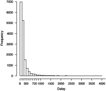
In the data the observed delay had a mean of 185 days, a little more than 6 months, and a standard deviation of 263 days. We want to fit a model to the data. We have fitted what we call a “claim delay distribution”. It gives you the probability that a claim which is diagnosed at age x, for a cause j, with risk factors θ, will be settled within a certain time of, say, u years.

Once we fit this distribution to the delay data, we can estimate the missing date of diagnosis. How can we do that? If we know the date of the settlement, then the date of diagnosis will be the date of settlement minus a point in time where the diagnosis happened and we could use the median of that distribution at that point in time. As we will see later on, we could use other measures or estimates of that distribution, but let us start with the median.

This will give you a value, a point estimate, of the date of diagnosis or of the waiting period between diagnosis and settlement of the claim. In Bayesian statistical modelling we have the entire distribution of the waiting time, so we can estimate other characteristics of our distribution, such as other percentiles.

We can use the claim delay distribution to adjust the exposure. We need to adjust the exposure for settlement and diagnosis of events.

We have also used office-specific growth rates in the modelling. This is to account for different companies changing in size, that is, changes in the number of policies that they sell throughout the 7 years for which we have data.

Figure 1 refers to the observed delay between diagnosis and settlement of the claim. It is a histogram of the data of that delay. As I said, the mean is about 185 days. You can see that it has a huge tail to the right. That delay, in practice, as has happened with the data, can be very long.

Figure 1

Claim settlement delay (days)

So far we have considered a model without taking into account any of the co-variates, the risk factors.

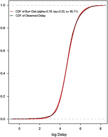
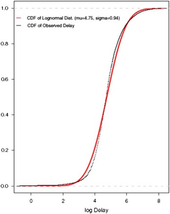
The black line is the observed distribution of the data. The red lines superimposed on it are two different distributions. Figure 2 is the Burr distribution and Figure 3 is a lognormal distribution fitted to the data without taking anything else into account.

Figure 2

Burr distribution fitted to settlement delay data

Figure 3

Lognormal distribution fitted to settlement delay data

It looks like the Burr distribution is giving a better fit to the data. Keep in mind that we have a lot of data here. We need to look into the details.

That was the result of fitting a model without taking into account any of the risk factors that I mentioned earlier.

Now I will show you how you can use what we call a linear model, or a model that looks like a generalised linear model (GLM), to take into account the different risk factors. I am going to show you four different models, referring to four different distributions, for the data.

Starting with a lognormal distribution and a translated gamma distribution, the probability functions take into account the risk factors. The mean of the delay now depends directly on the risk factors: age, sex, policy duration, type of policy and so on. It is straightforward to do this for a lognormal distribution using the GLM setting. We can also do it for a transformed gamma distribution and other distributions like the Burr distribution and the generalised beta distribution of the second kind.

I do not want to say any more at this stage about the probability functions. The key point is that we include all the co-variates – the risk factors – and the mean of the distribution depends on those risk factors.

We used Bayesian statistics to fit the models. We also used Markov chain Monte Carlo methods to fit the data. Without going into the details, I will give you a relative measure about how the models fit the data. This is a relative measure because we compare fit using the deviance information criterion. The smaller number means the better the fit of the distribution of the model to the data.

The generalised beta of the second kind gives the best fit to the data, followed by the Burr distribution, a three-parameter distribution, transformed gamma and the lognormal.

The generalised beta has four parameters and the Burr distribution has three parameters, the same as the transformed gamma. The lognormal has two parameters.

This measure takes into account the number of parameters. The larger the number of parameters, the more complex it is to fit the model.

The generalised beta distribution fits the data best but the lognormal is the easiest to use. That is important if you want to put this into practice.

Next is a comparison between the lognormal distribution and the Burr distribution.

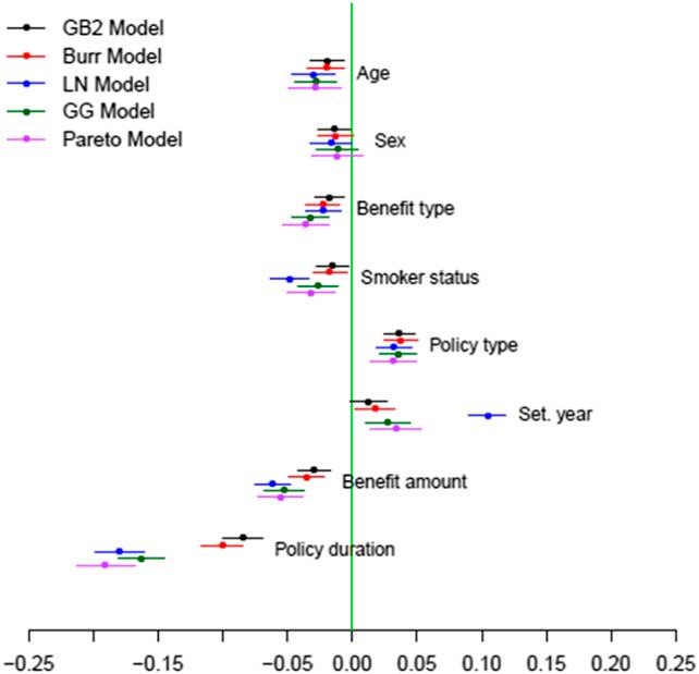
We are still looking at the delay distribution, the delay between diagnosis and settlement of the claim. We have the different risk factors in Figure 4. Each cluster of bars corresponds to different distributions that we have fitted. There are five here, one more than before. That is the Pareto distribution. Each bar corresponds to a 95% credible interval. It tells you about the uncertainty of the estimate of the coefficient of the age as a risk factor. The bullet in the middle of each interval is a mean of that estimate. That quantifies the uncertainty of those estimates.

Figure 4

Risk factor estimates

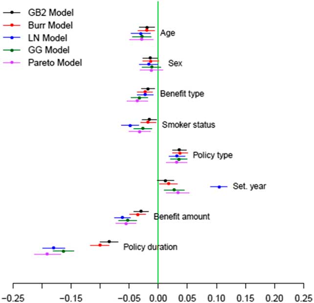
The green line in the middle of the plot is zero. If an interval is not crossed by the zero line, then this parameter plays a significant role to the delay distribution.

You can see that age is significant. The benefit type also has a significant effect. Most of the risk factors here have a significant effect.

We can see how differently these models perform in estimating those risk factors. For most of the risk factors you can see that the estimates are packed close together with a couple of exceptions, policy duration and settlement year, where you have a difference, when, for example, you fit a lognormal distribution. Generally, they do not give very different results from what we can see in the graph.

For example, benefit amount has a significant impact on the delay between the diagnosis and the settlement of the claim. I can see from this graph that it has a negative impact. That means that for the larger benefit amounts, the waiting time between diagnosis and settlement is shorter. It is the same with the policy duration. For younger policies, the waiting times are shorter.

Why do insurance companies settle higher claims faster? I do not have the answer to that, but that is what the data shows (Figure 5).

Figure 5

Illness coefficient estimates

This is the same graph but for the different illnesses that we are considering. Again, we have some that have a significant effect, for example, cancer and death. These have a negative impact on the length of the delay. In other words, claims on death are settled faster than other claims.

This may have a more obvious interpretation in terms of diagnosis of an event. It is much easier, obviously, to diagnose death than to diagnose, for example, permanent disability, which has a positive effect, or multiple sclerosis. These are illnesses that are much harder to diagnose, which also has an impact on how quickly these claims are settled.

Now consider a baseline scenario. This is a full accelerated policy on a joint life with a benefit amount of £50,000 sold by one particular office. The duration of the policy is 4 years. The claim was made on cancer.

Using the model we have fitted in this case – I think that this is based on the Burr model – the expected delay was 174 days with a 95% credible interval between 167 and 182 days.

I am now going to change each characteristic of the baseline case in turn. In the first one I am changing the benefit amount from £50,000 up to a quarter of a million pounds. The delay goes down significantly from 174 to 156 days on average with a credible interval of 146–166, which is significantly different from the previous interval.

From the reference scenario, I now change the duration of the policy from 4 years to 1 year. The waiting time for settlement goes up to 195 days. If you then change from cancer to death, it goes from 174 down to 112 days. On the other hand, if you change the cause of the claim from cancer to TPD, the average delay goes up to 217 days.

That gives you a numerical feel of how this model can predict the delay with different characteristics.

Let us now move on to estimation of the diagnosis rates. What I want to do here is estimate the intensity rate for a claim at age x, cause j and characteristic θ. This is a Poisson mortality model. The number of deaths have a Poisson distribution with a parameter that is given by the intensity rate times the exposure. This interval is the exposure.

What we are doing here is adjusting the exposure by using the probability that a claim is diagnosed and settled within the time window at which we are looking.

If you want to see how this would work in some sort of Markov-type model, we have two states. We have policyholders moving from the healthy state to the state of an insured event, which could be any illness or death. You can also distinguish between full accelerated and stand-alone policies – stand-alone policies are those that do not include death – by just splitting this state into two different states, diagnosed with an illness or death.

I want to estimate the intensity rate, the claim rate, λ. I am going to use what we call a Gompertz–Makeham–Cox-type model. We want to take into account age and all the different characteristics that we had before.

A Cox-type model has an additional term by comparison to a Gompertz–Makeham model. As it happens, with the data that we have, this term disappears from the model for all causes except death.

We can fit this model using usual statistical techniques. We can also then perform some variable selection to choose which of the risk factors are more important for claim rates.

Let us concentrate on the model that includes all causes. For this model, if we wanted to look at all possible diseases, then the important factors are age, the office through which the policy was sold, smoker status, and an interaction between age and smoking, which made sense in this case, and the policy duration. These are the most important risk factors for the rates.

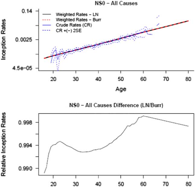
If you fit the two models corresponding to two different delay distributions – Figure 6 shows a Burr and a lognormal distribution for the delay – the claim rates are the function of age with age going from 20 up to roughly 80 on this first graph.

Figure 6

Claim rates for non-smokers, Pol Durn 0, all causes: Burr versus lognormal (LN)

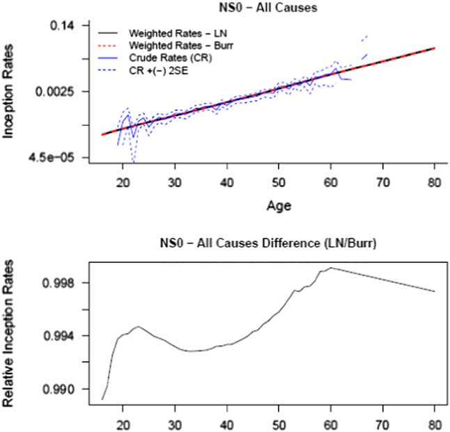
The blue lines are the crude rates, the observed rates. They jump around quite a lot. The black line corresponds to the model that uses the lognormal delay distribution. The red line corresponds to the model using the Burr delay distribution.

It is difficult to distinguish between the two lines, meaning that the two delay distributions give almost identical results in this case. That is important. On the second graph I have the relative rates. That is a ratio of the rate using the lognormal distribution divided by the rate using a Burr distribution. If the two rates were exactly the same, that ratio would always be equal to 1. There is only a 1% difference between the two models. These rates correspond to non-smokers with duration 0 and for all causes.

The rates for smokers are higher, as you might expect. Again, you cannot distinguish between the two distributions.

We have also looked at the sensitivity of this modelling to different estimates, using different point estimates of the delay distribution.

We have used the median of the delay distribution to estimate the waiting time, which works well, but we could use other percentiles of the distribution.

For example, if someone wanted to be conservative about the estimation, they might choose to use a 95^th percentile or even a 97.5^th percentile.

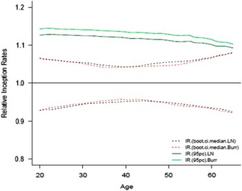
Figure 7 shows a line for different ages. The line at one is a relative rate. I have the rate that you can calculate if you use the median of the distribution divided by the rate that you obtain if you use any other percentile of the distribution. Obviously, for the median you get the line at one. We also have 95% bands around this line when you use the median of the delay distribution. The red one is the Burr, and the black one is the lognormal, as before.

Figure 7

Sensitivity to diagnosis estimates

If you use any other estimate up to the 95^th percentile, if you use any other point estimate of the delay distribution, the estimated claim rate will always be within this 95% interval.

The point estimate of the delay distribution is very small. The two green lines show what happens if you choose the 97.5^th percentile of the lognormal distribution to estimate the delay between diagnosis and settlement. This is when things start getting out of the 95% band of the estimation that we have here. It is quite robust.

I will now move on to pricing. What I have talked about until now is how we can use statistical modelling and Bayesian modelling to estimate the claim rate, and take into account uncertainty in the models and parameters. We can do the same for pricing. We can estimate the price that these policies need to be set at and can also include uncertainty.

We can calculate the net premium. This is an annual premium paid at constant rate on an n-year term. This will be given by this mathematical expression in Figure 8.

Figure 8

Annual premium estimation

You obviously need the benefit amount. This quantity involves the survival probability for a policyholder at age x. The λ is the same λ as the one that we estimated previously, the claim rate.

This probability will be known using life tables, λ we have estimated in the model already. For certain causes, certain characteristics, you can give a value to this net premium. That will be a single point estimate. But then I have a distribution for λ. We can derive the distribution for λ because we know about the uncertainty around it, using sophisticated methodology. If we know the distribution of λ then we can come up with the distribution of the net premium.

Let me give you some prices. Again, I am comparing two of the distributions for the claim delay: the lognormal and the Burr distribution. These prices are for a policyholder aged 40 with a policy duration 0. They refer to all causes with a benefit amount of £100,000 and an interest rate of 3%.

For a term of 25 years, the point estimate of the price is a net annual premium of £374 using the lognormal distribution for a non-smoker, with a corresponding confidence interval.

If you use a Burr distribution for the delay, the pricing goes slightly up from £374 to £382. There is a huge overlap in the confidence intervals of the two. That means that there is no significant change in the price that the policyholder will have to pay if you use one or the other distribution for a non-smoker.

The difference comes in when we consider smokers. Then the price goes from £374 to £714 with a lognormal distribution. There are similar numbers with a Burr distribution. These are now significantly different prices (Figure 9).

Figure 9

Premium pricing – comparisons

The graphs give you a summary of those prices. On the x axis you have the term of the policy. I am showing you how the price changes with respect to the term of the policy. The black line is using the lognormal model, the red line is using the Burr model and the dotted lines are 95% intervals around the point estimates.

The main message again, looking at non-smokers, is that there is a big overlap between the two intervals, meaning that there is no statistical difference between the price of the two models.

The difference comes when you consider smokers. These two graphs are not on the same scale. If I had them on the same scale you would see that the curves on the right would be well above the ones on the left. One goes up to £800, the other goes up to £400. There are significantly higher prices for smokers in this case.

You can have a model that considers all the different illnesses separately. Using such a model, you can come up with a claim rate or a price if you only wanted to know about premium rates for cancer. But that does not make sense. The way that critical illness works in the UK is that the critical illness will cover all of these illnesses. You cannot buy a policy that covers only cancer.

Insurance companies will sell policies that cover all of these illnesses. But perhaps not all of them – it has changed in recent years. Until very recently, it was quite common for a number of those companies not to include TPD. We want to see what happens if you take this out. You can do that if you consider all the causes separately and then take the TPD out of the equation.

The prices are slightly lower than the previous prices, meaning that for a product that would not include TPD, policyholders would pay slightly less – but not significantly less.

If you use one or the other of the two distributions that we have considered for the delay period, it will not make a significant difference in the premiums.

To summarise some of the points that I have tried to make here, I have spent some time talking about the delay between diagnosis and settlement in critical illness insurance. This delay time is important, especially if you think about claims that have occurred but are not settled yet, and the impact that this might have for reserves. We have developed a statistical model for that and fitted the model using a Bayesian methodology. This has allowed us to take into account the uncertainty in these models, the data and the parameters, and also to estimate non-recorded diagnosis dates.

We have used different distributions. The generalised beta distribution of the second kind gave the best fit to the data. The Burr distribution gave a very good fit. The lognormal distribution gave a reasonable fit and it is much simpler to use.

Based on that, we estimated smoothed critical illness rates. We included parameter and model uncertainty.

One of the main messages is that the claim delay distribution is model sensitive. But, if you are then thinking about claim rates and premiums, whether or not you use a Burr distribution or a generalised beta distribution of the second kind or the other two or three distributions that we have tested already does not make a difference. It is not statistically significant.

The Chairman: Thank you. We will now move on to the discussion part of the meeting.

Prof A. J. G. Cairns, F.F.A.: Thank you, Dr Streftaris, for an interesting and clear presentation. I have a couple of questions or points.

Towards the end you had the disaggregated estimates by individual causes. Did you do all of those separately and then add them to see whether you achieved the same results as if you were modelling all the causes at once?

Dr Streftaris: Yes, we did that. We obtained the estimates including all causes, and then using separate causes and adding up the different estimates. We did not check for confidence intervals, but for the point estimates we were very close to what you obtain with the two approaches.

Prof Cairns: Have I understood correctly that this is about the waiting distribution, which is always an important and challenging part of the exercise? In setting premium rates, I would guess that the waiting time is probably not going to make much of a difference. Perhaps I might be wrong on that count.

Where it does matter is how you estimate parameters for the actual diagnosis of other illnesses. That fed into the exposures. You were talking about the setting of the “incurred but not settled” reserves at the end. Are those the areas that are important versus the waiting time not being so important for premium setting?

Dr Streftaris: Yes, that is correct. We expected that to be the case. We expected that the claim delay distributions would play a bigger role in the first part of what I presented when we were talking about the impact of the delay on the “incurred but not reported” reserves, and so on.

However, an important aspect of this work was the missing diagnosis dates. For those, we had about 18% of the dates missing, I think. In an extreme case, where a huge percentage of diagnosis dates would be missing from the data, then we would have expected that distribution to play a bigger role also in the estimates of the claim rates and the premiums. This is because if you need to adjust the exposure, it depends more on the claim delay distribution if you do not know when the diagnosis happened.

As it is, we did know when the diagnosis happened in about 80% of the cases. That is one reason why the effect of that claim delay distribution was limited in the estimates of the claim rates and in the pricing.

But, you are right; you expect the contribution of that distribution in pricing to be smaller than in other aspects of this work.

Mr R. R. Ainslie, F.F.A: As an actuary, I think one moral of the story is, if you are a critical illness practitioner, you should be spending more time with your claims team, encouraging them to record diagnosis dates so you are not in the position of having to make a guess as to when this might have happened; 20% of claims without a diagnosis date is a remarkably high number when you think about it and the importance of this contract in financial services.

If you have not worked in critical illness insurance, you might be surprised to see that there are delays between settlement and diagnosis of up to half a year, which does seem somewhat shocking. You would think that if you had had a heart attack, the benefit would be paid out straightaway. But the reality for claims professionals is that they have to look at and check various things, including non-disclosure and whether a particular definition been satisfied?

With that in mind, especially with the work on non-disclosure, and the amount of time claims managers spend checking back through records, I was surprised to see that policy duration was only a significant factor, it seemed, for two or three of the illnesses.

Across all claims you would expect to examine a new claim more thoroughly as a claims manager than one which had been on the books for 10 years, hence I might have expected more of a duration-related effect.

Dr Streftaris: That is a good point. Policy duration was, if we look at the model that included all causes, a significant factor.

If you look at different causes separately, there are also issues about how much data you have for each separate cause, and so on. So things might be slightly distorted if you are looking at specific causes.

I agree that if you look at the delay being long between diagnosis and settlement, you do need to take into account things that you mentioned such as disclosure issues. Also, some of the illnesses are much easier to diagnose than others.

The medical profession has to come into this as well and confirm an illness. There is a question about when an illness really starts, because that is the diagnosis date. If we are talking about disability, multiple sclerosis or even cancer in some cases, that is not an easy question to answer. There is a delay definitely between diagnosis and settlement.

I am not claiming that this delay is a fault of the insurance companies. I am saying that the specifics of this insurance product are such that those claim delays will exist. So, it is good to be able to model that delay.

Mr J. Taylor, F.F.A: I am interested in the possibility of decomposing the delay into the gap between medical diagnosis and claim being submitted through them to settlement. I wonder whether you have sufficient data to do that and whether it would yield any insight.

For example, you showed that higher benefit claims were settled more quickly. I wonder if that is symptomatic of higher net worth consumers using advisers who then submit prompt claims, rather than, say, insurance companies settling more quickly.

Dr Streftaris: That is interesting. We have not looked at that point in detail. We have a date of diagnosis, or we do not have a date of diagnosis. Also, we consider the date of notification, the date of admission before settlement. There is a timeline for a claim from the time it is diagnosed until settlement.

We have some information on other events, perhaps not the one you mentioned about medical notification, and so on. We did have some information on that but we have not modelled it.

Professor Waters or Dr Dodd will perhaps correct me if this is not true, but I do not think we had enough data to be able to model them. It was not a primary aim to look at that when we started this work. However, it can definitely decompose into different intervals.

Mr J. K. Wilson, F.I.A.: I wondered, when you produced the incidence rates, did you do any comparison against the rates introduced by the CMI? They have produced an insurer’s life table. I do not think the data period exactly matches. I think it is between 2002 and 2006.

Dr Streftaris: Yes, we have done some comparisons. One of the reasons why I was presenting the Burr distribution here, together with a lognormal, rather than the best fit distribution, the generalised beta of the second kind, was because the Actuarial Profession has published some results using the Burr distribution.

Our results are quite similar to the results that the Institute and Faculty has published. One difference is that the work that has been published in Actuarial Profession working papers does not go into the same detail as the work that ours has in terms of the different factors, or at least not putting all of them in a coherent model.

Prof H. R. Waters, F.F.A.: Just a couple of points. The missing dates of diagnosis – about 20%: I think that percentage is going down over time and perhaps the quality of data is improving.

Policy duration was mentioned. One of the factors here was when we looked at individual causes, policy duration mattered for the delay for TPD and for multiple sclerosis only.

For those two illnesses, the standard definition from the ABI says 6 months of continuous symptoms. So, a diagnosis at the beginning, 6 months of continuous symptoms and a diagnosis confirmed at the end. We assumed the insurance company would put the date of diagnosis at the end of that 6-month period.

Automatically that means that you have very few claims for those causes of duration 0.

Mr Taylor mentioned the different dates. The data showed, in ideal cases, the date of diagnosis, the date of notification to the insurance company, the date that the insurance company admitted that the claim was valid and then the date that the claim was settled.

Typically, there was a short delay between admission and settlement. The insurance company would pay up quickly after they had admitted it. The data was far from complete. We had date of settlement for more or less everything. The insurance companies were keen to record when they had paid money.

But the insured event is diagnosis. That was what we needed and that was a problem.

We did have this other data but it was patchy. We could have used it. It would have been a different modelling exercise if we had done that.

Mr K. J. Tindall, F.F.A.: I think that the data you are using is 10–15-years-old. What is the applicability of your results to now, given the data is somewhat out-of-date?

In my mind, the ability to diagnose will have changed. But does that affect the claim delay or does that affect the quantum of the premium that we would charge? You may know more diseases exist as opposed to making notification any quicker.

Maybe some insurers are moving towards online notification to reduce the claim delay. Do you think that that will have any impact on your results?

Were there any risk factors for which you would have liked to have had data that would have improved your model? For example, marital status potentially could be a risk factor. Would marital status have sped up the notification process and the payment process? I am not sure.

Dr Streftaris: You are right. The data goes back some time ago. I accept that things have been changing, and are changing, in terms of how quickly insurance companies react and respond to these claims.

The data that we have goes up to 2005. I know that the Institute and Faculty, or the CMI, has collected more recent data, up to 2012. We have been in talks with them to get hold of the data and update our results.

We expect changes will have happened since the period to which our data refers. You mentioned improvements in diagnosis of illnesses. That definitely will have an impact, mainly on the delay distribution rather than the pricing. We want to consider more recent data and see how these will change our estimates.

Also, you mentioned online notification. I believe that will have an impact. This also part answers your last question about what other risk factors we would like to have. This might then be another co-variate. How the claim is made or is notified, if it is made online, through a letter or other routes. That might be something that affects these delays. That is something, if we had that information, we could have taken into account.

The trouble here is that we do not choose which risk factors, which co-variates, what information, we can use. This was already collected when we obtained the data. It is a rather sensitive matter of having the data available. It is not as easy as you might think.

Mr Ainslie: Just to pick up on that as a discussion point, I think that you would intuitively expect to see a significant difference between the period that the data refers to and the current period over the last 2 or 3 years for claims, primarily because of the impact of the agreement between the ABI and the Financial Ombudsman Service.

That has fundamentally changed the way that insurance companies face up to disputed claims. We have seen over that period that the number of claims that has been declined has reduced markedly. You have a different mix of types of claims being paid now as there were back, say, in 1998 and 1999.

The second major factor that you would see in the difference between then and now is perhaps not so much the online notification, which intuitively should not make that much of a difference, but settling claims more rapidly. Insurance companies are making far more effort perhaps to pay the money out before, for example, legal title has been fully established.

That is one of the main reasons why death claims are so greatly delayed: establishing to whom the money should legally go.

The Chairman: It remains for me to express my thanks to all of you who have participated in this evening’s discussion. I would particularly like to thank our speaker and I ask you to show your appreciation.