1. Introduction
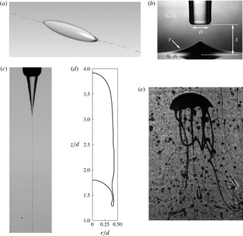
There are many types of flows in which the interface between two immiscible fluids sheds small drops with length scales much smaller than those characterizing the parent fluid mass. An early and famous example is the flow observed by Taylor (Reference Taylor1934) in his four-roller mill in which, under certain conditions, a drop in a hyperbolic flow field was seen to emit threads which eventually broke up into much smaller drops with a diameter of the order of 1 % of that of the original drop. This so-called ‘tip-streaming’ phenomenon was later found to be strongly favoured by surfactants and electric fields and has been extensively investigated; see e.g. Sherwood (Reference Sherwood1984), de Bruijn (Reference de Bruijn1993), Eggleton, Tsai & Stebe (Reference Eggleton, Tsai and Stebe2001), Mulligan & Rothstein (Reference Mulligan and Rothstein2011), Collins et al. (Reference Collins, Krishnaraj, Harris and Basaran2013). An example from Adami, Hu & Adams (Reference Adami, Hu and Adams2010) is shown in figure 1(a).
Examples of fluid–fluid flows giving rise to small structures detached or about to detach. (a) Tip-streaming from a drop in simple shear flow in the presence of surfactants (from Adami et al.
Reference Adami, Hu and Adams2010). (b) Cusp-like structure on the plane interface separating heavy mineral oil (above) and a water–glycerin mixture when the oil is selectively withdrawn; the tube inner diameter is 16 mm (from Cohen & Nagel Reference Cohen and Nagel2002). (c) Water drops generated within a faster co-flowing stream of a silicon oil (viscosity
 $0.1~\text{N}~\text{s}~\text{m}^{-2}$
); the outer diameter of the tube is
 $200~{\rm\mu}\text{m}$
and the capillary number based on the outer fluid velocity and properties is 1.12 (from Gordillo, Sevilla & Campo-Cortes Reference Gordillo, Sevilla and Campo-Cortes2014). (d) Skirt-like appendage at the bottom of an axisymmetric gas bubble rising in a tube; the Morton number is
 $3.6\times 10^{-4}$
and the Eötvös number is 300 (from Lu & Prosperetti Reference Lu and Prosperetti2009). (e) Oil filaments trailing a surfactant-covered oil drop rising in water; the drop width is about 3 mm (J. Katz, private communication).

Another instance of the same phenomenon, illustrated in figure 1(b), is the cusp-like structure forming on the plane interface separating two immiscible liquids when the upper one is selectively withdrawn by a tube; see e.g. Cohen & Nagel (Reference Cohen and Nagel2002), Blanchette & Zhang (Reference Blanchette and Zhang2009).
Yet another instance occurs when a liquid jet enters a coaxially and more rapidly flowing immiscible liquid. In suitable conditions the tip of the jet becomes pointed until a very thin filament, which ultimately breaks up into small drops, issues from it; an example from Gordillo et al. (Reference Gordillo, Sevilla and Campo-Cortes2014) is shown in figure 1(c). This arrangement, referred to as flow focusing, has recently become the object of intense research in view of its importance for many microfluidic applications; see e.g. Basaran (Reference Basaran2002), Anna, Bontoux & Stone (Reference Anna, Bontoux and Stone2003), Barrero & Loscertales (Reference Barrero and Loscertales2007), Marín, Campo-Cortés & Gordillo (Reference Marín, Campo-Cortés and Gordillo2009), Jeong et al. (Reference Jeong, Lim, Choi, Kim, Lee, Kim, Lee, Kim, Yi and Yang2012).
A related example is the well-known phenomenon of ‘skirts’ that are sometimes found issuing from the rim of drops or bubbles moving in a host liquid under the action of buoyancy; see e.g. Thomson & Newall (Reference Thomson and Newall1885), Bhaga & Weber (Reference Bhaga and Weber1981). The skirt may either remain attached or separate and subsequently break up; a numerical simulation of the two-dimensional analogue of incipient skirt formation is shown later in figure 23. These thin structures can also form in a confined flow at the micro-scale (see e.g. Mulligan & Rothstein Reference Mulligan and Rothstein2011) or at larger scales such as behind Taylor bubbles; the latter situation is shown in figure 1(d) from Lu & Prosperetti (Reference Lu and Prosperetti2009).
As shown in figure 1(a), surfactants have a dramatic effect on the formation of filaments and shedding of drops. A striking example is provided by figure 1(e), in which thin filaments are seen to detach from a surfactant-covered oil drop rising in water (J. Katz, private communication; see also Gopalan & Katz Reference Gopalan and Katz2010). This particular study is part of an effort to understand the action of surface-active dispersants on oil spills in the ocean, as extensively carried out, for example, on the damaged Macondo well on the occasion of the 2010 Deepwater Horizon accident. This practice is intended to exploit the fragmentation process to reduce the size of the oil globules released in the water column. It is thought that the resulting improved mixing would lessen the potential for contamination of shoreline habitats and coastal ecosystems and, at the same time, accelerate the rate of biodegradation (see e.g. OSCA 2011).
In the present paper we point out that these diverse phenomena are the result of a generic instability that affects the interface separating two immiscible fluids near points (or lines) where the vorticity vanishes. A schematic explanation of the mechanism for this instability is provided in figure 2, which shows the typical structure of the flow in the neighbourhood of such a point. Under the action of the fluid motion, a small perturbation on the interface is forced to grow both by the kinematic compression due to the converging velocity field, and by the dynamic effects of the viscous shear stress exerted by the fluid into which it protrudes, together with the surrounding pressure field. The mechanism opposing the growth of the instability is the action of surface tension, which is strongly inhibited by the presence of surfactants. The kinematic aspect of this instability is well known, for example, in the context of spherical flows, as in the case of a collapsing bubble (see e.g. Plesset Reference Plesset1954; Hao & Prosperetti Reference Hao and Prosperetti1999). If the flow is directed away from the zero-vorticity point, on the other hand, the kinematic effect stabilizes the interface, as shown, for example, by Frankel & Weihs (Reference Frankel and Weihs1985), who studied the stability of a stretching jet.
Qualitative explanation of the instability object of the present study. The flow near the zero vorticity point
 $O$
can be convergent or divergent. In the former case, illustrated here, a local perturbation can grow due to kinematic compression and viscous stresses. If surfactants are present, they are carried by the flow toward the zero-vorticity point and weaken the action of surface tension, which is the only physical mechanism countering the instability.

There are many other instances, of course, in which the formation of small drops or bubbles is the result of a different mechanism, such as viscous shear in a stratified flow, splashing or the capillary break-up of the stem connecting the two parts of a drop which is about to split. The considerations that follow have no bearing on such cases.
We start with a study of the unperturbed base flow near a zero-vorticity point in the two-dimensional case. It will be argued that the results of this analysis also have a bearing on the three-dimensional flow in the neighbourhood of a line along which the vorticity tangent to the interface vanishes. The analysis of the general three-dimensional situation cannot be carried to the same level of detail, but sufficient arguments are provided in appendix B to show that an instability of a similar nature can be expected here too and, in particular, near a point on the axis of symmetry in three dimensions as in figure 1(a–c).
We then carry out an approximate linearized stability analysis near the two-dimensional zero-vorticity point, which is later on supported and illustrated by numerical computations. We briefly show the effect of surfactants, both soluble and insoluble, and conclude with a numerical illustration of how the idealized flow structure near the zero-vorticity point is embedded into two actual flows, a flow-focusing-like system of coaxial jets and the development of a skirt behind a translating drop.
2. Mathematical model
We consider a two-dimensional version of the problem in which two semi-infinite fluids are separated by an interface specified as
 $$\begin{eqnarray}S(x,y,t)\equiv y-{\it\eta}(x,t)=0.\end{eqnarray}$$
The undisturbed interface is at
 $y=0$
and
 ${\it\eta}$
represents its deformation. The two fluids are incompressible, so that their velocity fields,
 $\boldsymbol{u}$
, are solenoidal:
 $$\begin{eqnarray}\boldsymbol{{\rm\nabla}}\boldsymbol{\cdot }\boldsymbol{u}=0.\end{eqnarray}$$
Since we are interested in the small-scale local flow in the neighbourhood of a specific point on the interface, we are justified in neglecting body forces so that the momentum equation reduces to
 $$\begin{eqnarray}\partial _{t}\boldsymbol{u}+\boldsymbol{u}\boldsymbol{\cdot }\boldsymbol{{\rm\nabla}}\boldsymbol{u}=-\frac{1}{{\it\rho}}\boldsymbol{{\rm\nabla}}p+{\it\nu}{\rm\nabla}^{2}\boldsymbol{u},\end{eqnarray}$$
in which
 ${\it\rho}$
and
 $p$
are the density and pressure and
 ${\it\nu}={\it\mu}/{\it\rho}$
is the kinematic viscosity defined by the ratio of the dynamic viscosity
 ${\it\mu}$
to the density.
The kinematic condition requires that, on
 $S=0$
, both velocity fields satisfy
 $$\begin{eqnarray}-\partial _{t}{\it\eta}+\boldsymbol{u}\boldsymbol{\cdot }\boldsymbol{{\rm\nabla}}S=0.\end{eqnarray}$$
The condition on the normal stresses is
 $$\begin{eqnarray}-p_{u}+p_{l}+\boldsymbol{n}\boldsymbol{\cdot }{\bf\tau}_{u}\boldsymbol{\cdot }\boldsymbol{n}-\boldsymbol{n}\boldsymbol{\cdot }{\bf\tau}_{l}\boldsymbol{\cdot }\boldsymbol{n}={\it\sigma}\boldsymbol{{\rm\nabla}}\boldsymbol{\cdot }\boldsymbol{n},\end{eqnarray}$$
where
 ${\bf\tau}$
is the viscous stress and
 ${\it\sigma}$
the surface tension coefficient; here and for the rest of the paper the subscripts
 $u$
and
 $l$
refer to the upper and lower fluid, respectively. As long as we do not consider surfactants, the tangential stresses must be continuous at the interface; continuity of the tangential velocity is also imposed.
3. Local analysis
We begin by carrying out a linearized stability analysis of the surfactant-free case in the neighbourhood of a two-dimensional zero-vorticity point on a flat interface separating two incompressible fluids. We assume that this point is at rest, if necessary by carrying out a Galilean transformation. Since vorticity vanishes, the transformation is purely translatory, and apparent forces that it might introduce can be accounted for by a modified pressure. This procedure is exact only when the two fluids have equal densities, but the error may be expected to be small in the case of liquid–liquid systems in view of the small density differences between many common liquids, such as oil and water, and of the small accelerations typically encountered in the flows of present concern. We also assume that the unperturbed flow is steady. Velocities are small near the stagnation point and therefore, for simplicity, we neglect the non-linear term in the Navier–Stokes equation (2.3). A numerical example in which this approximation is not adopted is presented at the end of § 4, where it is found that the error incurred is small. We first derive expressions for the local structure of the undisturbed flow near the zero-vorticity point, and then carry out the perturbation analysis.
3.1. Base flow
Let
 ${\it\Psi}_{u,l}$
be the stream functions describing the undisturbed flow in the upper and lower fluids, respectively, and expand them in a Taylor series near the origin. After imposing the continuity of velocity and of the tangential stress across the undisturbed plane surface
 $y=0$
separating the two fluids, we find
 $$\begin{eqnarray}\displaystyle & {\it\Psi}_{u}(x,y)=-Axy+{\textstyle \frac{1}{6}}By^{3}+{\textstyle \frac{1}{2}}Cx^{2}y+{\textstyle \frac{1}{2}}Dxy^{2}+\cdots \,, & \displaystyle\end{eqnarray}$$
 $$\begin{eqnarray}\displaystyle & {\it\Psi}_{l}(x,y)=-Axy+{\textstyle \frac{1}{6}}[{\it\mu}B+3({\it\mu}-1)C]y^{3}+{\textstyle \frac{1}{2}}Cx^{2}y+{\textstyle \frac{1}{2}}{\it\mu}Dxy^{2}+\cdots \,, & \displaystyle\end{eqnarray}$$
 $$\begin{eqnarray}{\it\mu}=\frac{{\it\mu}_{u}}{{\it\mu}_{l}},\end{eqnarray}$$
and
 $$\begin{eqnarray}A=-\partial _{x}\partial _{y}{\it\Psi}_{u},\quad B=\partial _{y}^{3}{\it\Psi}_{u},\quad C=\partial _{x}^{2}\partial _{y}{\it\Psi}_{u},\quad D=\partial _{x}\partial _{y}^{2}{\it\Psi}_{u},\end{eqnarray}$$
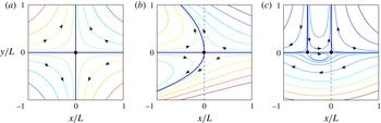
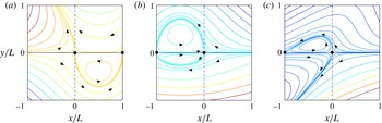
all evaluated at the origin. Equations (3.1) and (3.2) are the most general form of the stream functions near a two-dimensional zero-vorticity point at rest on a plane interface, taken as the origin. Several examples of streamlines corresponding to different values of the parameters are shown in figures 3 and 4 and additional details on the flow are provided in appendix A.
Examples of streamlines of the base flow
 ${\it\mu}_{u}/{\it\mu}_{l}=3$
and
 $A>0$
: (a)
 $B=C=D=0$
; (b)
 $B<0$
and
 $C=D=0$
; (c)
 $C<0$
and
 $B=D=0$
. The zero-vorticity stagnation point is marked by a dot at the origin. In (c) the black square marks the second stagnation point that exists in this case; vorticity at this point (which is stable as the flow is directed away from it) does not vanish.

Examples of streamlines of the base flow
 ${\it\mu}_{u}/{\it\mu}_{l}=3$
and
 $A>0$
,
 $B=-3A/L$
: (a)
 $C=2A/L$
and
 $D=0$
; (b)
 $C=-2A/L$
and
 $D=0$
; (c)
 $C=-2A/L$
and
 $D=3A/L$
.

The upper-fluid horizontal,
 $U_{u}$
, and vertical,
 $V_{u}$
, velocity components are
 $$\begin{eqnarray}U_{u}=-Ax+{\textstyle \frac{1}{2}}By^{2}+{\textstyle \frac{1}{2}}Cx^{2}+Dxy,\quad V_{u}=Ay-Cxy-{\textstyle \frac{1}{2}}Dy^{2},\end{eqnarray}$$
and the corresponding lower-fluid ones are
 $$\begin{eqnarray}U_{l}=-Ax+{\textstyle \frac{1}{2}}({\it\mu}B+3({\it\mu}-1)C)y^{2}+{\textstyle \frac{1}{2}}Cx^{2}+{\it\mu}Dxy,\quad V_{l}=Ay-Cxy-{\textstyle \frac{1}{2}}{\it\mu}Dy^{2}.\end{eqnarray}$$
The root of the instability is contained in the first terms of
 $U_{u,l}$
when
 $A>0$
, which are the two-dimensional analogue, for example, of the hyperbolic flow of Taylor’s four-roller mill (see (3.9) below).
The unperturbed pressure,
 $P_{u}$
, and vorticity,
 $Z_{u}$
, fields in the upper fluid are
 $$\begin{eqnarray}P_{u}={\it\mu}_{u}[(B+C)x-Dy],\quad Z_{u}=-Dx-(B+C)y,\end{eqnarray}$$
while, in the lower fluid,
 $$\begin{eqnarray}\displaystyle & P_{l}=-2({\it\mu}_{u}-{\it\mu}_{l})A+[{\it\mu}_{u}B+(3{\it\mu}_{u}-2{\it\mu}_{l})C]x-{\it\mu}_{u}Dy, & \displaystyle\end{eqnarray}$$
 $$\begin{eqnarray}\displaystyle & Z_{l}=-{\it\mu}Dx-[{\it\mu}B+(3{\it\mu}-2)C]y. & \displaystyle\end{eqnarray}$$
As shown in appendix B, for a three-dimensional flow symmetric around an axis through a point normal to the interface, the velocity components near that point are given by
 $$\begin{eqnarray}U_{r}\simeq -{\textstyle \frac{1}{2}}Ar,\quad U_{z}=Az,\end{eqnarray}$$
where
 $U_{r}$
and
 $U_{z}$
are the radial and normal velocity components in a meridian plane. This flow, which is relevant to figure 1(a–c), is clearly very similar to that depicted in figure 3(a), and therefore qualitatively similar conclusions to those to be drawn here may be expected to apply to this case as well.
For more general three-dimensional situations it is not possible to carry out as exhaustive an analysis as that above. Some partial results, given in appendix B, show that, near a three-dimensional zero-vorticity point, flows with a structure similar to (3.9) and to that found in two dimensions can also exist. Given that, as illustrated in figure 2, the instability is rooted in the convergent kinematics of the base flow, these results support the applicability of the present interpretation to three-dimensional flows as well. If, instead of a point, the vorticity tangent to the interface vanishes along a smooth line, as in figure 1(d,e), the flow can be approximated by a two-dimensional flow similar to that described earlier in a plane normal to the line, up to distances that are small compared with the inverse curvature and torsion of the line. An example is the flow that develops on the lower side of a rising bubble or drop when the outer flow separates (see § 6 and figure 23 below). An instability similar to that described in the analysis that follows may therefore be expected in this case as well, as suggested by figure 1(d,e).
3.2. Linearization
Linearization of the kinematic condition (2.1) gives
 $$\begin{eqnarray}\partial _{t}{\it\eta}+U_{u,l}(x,0)\partial _{x}{\it\eta}=v_{u,l}|_{y=0},\end{eqnarray}$$
where
 $v_{u,l}$
is the perturbation velocity in the
 $y$
direction in the upper and lower fluid, respectively. The continuity of tangential velocities stipulates that
 $$\begin{eqnarray}[u_{l}-u_{u}]_{y=0}=(1-{\it\mu})Dx{\it\eta},\end{eqnarray}$$
where
 $u_{u,l}$
is the perturbation velocity in the
 $x$
direction. Continuity of tangential stresses requires that
 $$\begin{eqnarray}[{\it\tau}_{l,xy}-{\it\tau}_{u,xy}]_{y=0}=4({\it\mu}_{l}-{\it\mu}_{u})(-A+Cx)\partial _{x}{\it\eta}+4({\it\mu}_{l}-{\it\mu}_{u})C{\it\eta},\end{eqnarray}$$
where
 ${\it\tau}_{xy}={\it\mu}[\partial _{y}u+\partial _{x}v]$
, while the jump in normal stresses is given by
 $$\begin{eqnarray}[\,p_{l}-p_{u}+{\it\tau}_{uyy}-{\it\tau}_{l,yy}]_{y=0}=-{\it\sigma}\partial _{x}^{2}{\it\eta}.\end{eqnarray}$$
The presence of the independent variable
 $x$
in some terms of these equations prevents a simple solution to the problem. However, in the immediate neighbourhood of the origin,
 $x$
is small, so these terms are small and we are justified in dropping them; their effect will be investigated numerically in the next section.
3.3. Solution
The removal of terms explicitly dependent on
 $x$
permits us to look for solutions of the perturbation problem depending on
 $x$
and time, proportional to
 $\text{e}^{\text{i}(kx-{\it\omega}t)}$
. Thus, the perturbation vorticity equation
 $$\begin{eqnarray}\partial _{t}{\it\zeta}={\it\nu}{\rm\nabla}^{2}{\it\zeta}\end{eqnarray}$$
takes the form
 $$\begin{eqnarray}\partial _{y}^{2}{\it\zeta}_{u,l}-(k^{2}-{\it\lambda}_{u,l}^{2}){\it\zeta}_{u,l}=0,\quad \text{with}~{\it\lambda}_{u,l}^{2}=\frac{\text{i}{\it\omega}}{{\it\nu}_{u,l}}.\end{eqnarray}$$
Upon integration of
 ${\rm\nabla}^{2}{\it\psi}=-{\it\zeta}$
subject to the appropriate boundary conditions at infinity, with
 ${\it\psi}$
the perturbation stream function, we find
 $$\begin{eqnarray}{\it\psi}_{u}=\frac{1}{2k}\left[{\it\alpha}_{u}(x,t)\text{e}^{-ky}+\frac{2k}{{\it\lambda}_{u}^{2}}\,{\it\zeta}_{u}^{0}\text{e}^{-\sqrt{k^{2}-{\it\lambda}_{u}^{2}}y}\right],\end{eqnarray}$$
and
 $$\begin{eqnarray}{\it\psi}_{l}=\frac{1}{2k}\left[{\it\alpha}_{l}(x,t)\text{e}^{ky}+\frac{2k}{{\it\lambda}_{l}^{2}}\,{\it\zeta}_{l}^{0}\text{e}^{\sqrt{k^{2}-{\it\lambda}_{l}^{2}}y}\right].\end{eqnarray}$$
Here
 ${\it\alpha}_{u,l}$
and
 ${\it\zeta}_{u,l}^{0}$
are integration constants (in the sense that they are independent of
 $y$
although they contain the factor
 $\text{e}^{\text{i}(kx-{\it\omega}t)}$
), with the last pair being the perturbation vorticity at the interface. The corresponding perturbation velocity components and pressure in the upper fluid are
 $$\begin{eqnarray}\displaystyle & \displaystyle u_{u}=\frac{1}{2k}\left[-k{\it\alpha}_{u}\text{e}^{-ky}-\frac{2k}{{\it\lambda}_{u}^{2}}\sqrt{k^{2}-{\it\lambda}_{u}^{2}}\,{\it\zeta}_{u}^{0}\text{e}^{-\sqrt{k^{2}-{\it\lambda}_{u}^{2}}y}\right], & \displaystyle\end{eqnarray}$$
 $$\begin{eqnarray}\displaystyle & \displaystyle v_{u}=-\frac{\text{i}}{2}\left[{\it\alpha}_{u}\text{e}^{-ky}+\frac{2k}{{\it\lambda}_{u}^{2}}\,{\it\zeta}_{u}^{0}\text{e}^{-\sqrt{k^{2}-{\it\lambda}_{u}^{2}}y}\right], & \displaystyle\end{eqnarray}$$
 $$\begin{eqnarray}\displaystyle & \displaystyle p_{u}=\text{i}\frac{{\it\mu}_{u}{\it\lambda}_{u}^{2}}{2k}{\it\alpha}_{u}\text{e}^{-ky}, & \displaystyle\end{eqnarray}$$
 $$\begin{eqnarray}\displaystyle & \displaystyle u_{l}=\frac{1}{2k}\left[k{\it\alpha}_{l}\text{e}^{ky}+\frac{2k}{{\it\lambda}_{l}^{2}}\,\sqrt{k^{2}-{\it\lambda}_{l}^{2}}\,{\it\zeta}_{l}^{0}\text{e}^{\sqrt{k^{2}-{\it\lambda}_{l}^{2}}y}\right], & \displaystyle\end{eqnarray}$$
 $$\begin{eqnarray}\displaystyle & \displaystyle v_{l}=-\frac{\text{i}}{2}\left[{\it\alpha}_{l}\text{e}^{ky}+\frac{2k}{{\it\lambda}_{l}^{2}}\,{\it\zeta}_{l}^{0}\text{e}^{\sqrt{k^{2}-{\it\lambda}_{l}^{2}}y}\right], & \displaystyle\end{eqnarray}$$
 $$\begin{eqnarray}\displaystyle & \displaystyle p_{l}=-\text{i}{\it\mu}_{l}\frac{{\it\lambda}_{l}^{2}}{2k}{\it\alpha}_{l}\text{e}^{ky}. & \displaystyle\end{eqnarray}$$
For both fluids the kinematic condition (3.10) simplifies to
 $(-A-\text{i}{\it\omega}){\it\eta}+\text{i}k{\it\psi}=0$
, from which
 $$\begin{eqnarray}\frac{\text{i}}{2}\left({\it\alpha}_{u}+\frac{2k}{{\it\lambda}_{u}^{2}}\,{\it\zeta}_{u}^{0}\right)=(\text{i}{\it\omega}+A){\it\eta},\quad \frac{\text{i}}{2}\left({\it\alpha}_{l}+\frac{2k}{{\it\lambda}_{l}^{2}}\,{\it\zeta}_{l}^{0}\right)=(\text{i}{\it\omega}+A){\it\eta},\end{eqnarray}$$
which permit us to express
 ${\it\alpha}_{u,l}$
in terms of
 ${\it\zeta}_{l,u}^{0}$
:
 $$\begin{eqnarray}{\it\alpha}_{u,l}=2({\it\omega}-\text{i}A)-\frac{k}{{\it\lambda}_{u,l}^{2}}{\it\zeta}_{u,l}^{0}.\end{eqnarray}$$
With this step, the condition of continuity of the tangential velocity becomes
 $$\begin{eqnarray}2({\it\omega}-A\text{i}){\it\eta}+\frac{\sqrt{k^{2}-{\it\lambda}_{l}^{2}}-k}{{\it\lambda}_{l}^{2}}\,{\it\zeta}_{l}^{0}+\frac{\sqrt{k^{2}-{\it\lambda}_{u}^{2}}-k}{{\it\lambda}_{u}^{2}}\,{\it\zeta}_{u}^{0}=0,\end{eqnarray}$$
and that for the tangential stress
 $$\begin{eqnarray}{\it\mu}_{u}{\it\zeta}_{u}^{0}-{\it\mu}_{l}{\it\zeta}_{l}^{0}=2({\it\mu}_{l}-{\it\mu}_{u})(-\text{i}kA+2C-k{\it\omega}){\it\eta}.\end{eqnarray}$$
Finally, the normal stress condition becomes
 $$\begin{eqnarray}\displaystyle & & \displaystyle \left[-{\it\sigma}k^{2}+2\text{i}{\it\mu}_{l}\left(k-\frac{{\it\lambda}_{l}^{2}}{2k}\right)({\it\omega}-A\text{i})+2\text{i}{\it\mu}_{u}\left(k-\frac{{\it\lambda}_{u}^{2}}{2k}\right)({\it\omega}-A\text{i})\right]{\it\eta}\nonumber\\ \displaystyle & & \displaystyle \quad +\,\text{i}{\it\mu}_{l}\left[1-\frac{2k}{{\it\lambda}_{l}^{2}}\left(k-\sqrt{k^{2}-{\it\lambda}_{l}^{2}}\right)\right]{\it\zeta}_{l}^{0}+\text{i}{\it\mu}_{u}\left[1-\frac{2k}{{\it\lambda}_{u}^{2}}\left(k-\sqrt{k^{2}-{\it\lambda}_{u}^{2}}\right)\right]{\it\zeta}_{u}^{0}=0.\nonumber\\ \displaystyle & & \displaystyle\end{eqnarray}$$
3.4. Characteristic equation
The condition for the existence of a non-zero solution to the homogeneous algebraic system (3.26), (3.27) and (3.28) gives the characteristic equation
 $$\begin{eqnarray}c_{1}({\it\omega}^{2}-{\it\omega}_{0}^{2})-\text{i}c_{2}{\it\omega}+4c_{3}=0,\end{eqnarray}$$
in which
 $$\begin{eqnarray}{\it\omega}_{0}^{2}=\frac{{\it\sigma}}{{\it\rho}_{l}+{\it\rho}_{u}}k^{3}\end{eqnarray}$$
is the angular frequency for capillary waves at the interface of two inviscid fluids, and
 $$\begin{eqnarray}\displaystyle & \displaystyle c_{1}=\frac{{\it\rho}_{u}+{\it\rho}_{l}}{k^{2}{\it\mu}_{l}}(R_{u}+{\it\mu}R_{l}), & \displaystyle\end{eqnarray}$$
 $$\begin{eqnarray}\displaystyle & \displaystyle c_{2}=\frac{{\it\rho}_{u}+{\it\rho}_{l}}{k^{2}{\it\mu}_{l}}(R_{u}+{\it\mu}R_{l})A-4[{\it\mu}+(1-{\it\mu})R_{u}][1-(1-{\it\mu})R_{l}], & \displaystyle\end{eqnarray}$$
 $$\begin{eqnarray}\displaystyle & \displaystyle c_{3}=[{\it\mu}+(1-{\it\mu})^{2}R_{u}R_{l}]A-\text{i}\frac{1-{\it\mu}}{k}[R_{u}-{\it\mu}R_{l}-2(1-{\it\mu})R_{u}R_{l}]C, & \displaystyle\end{eqnarray}$$
 $$\begin{eqnarray}R_{u,l}=k\frac{k-\sqrt{k^{2}-{\it\lambda}_{u,l}^{2}}}{{\it\lambda}_{u,l}^{2}}.\end{eqnarray}$$
It is readily checked that, if
 ${\it\mu}_{u}={\it\mu}_{l}$
, the characteristic equation (3.29) is invariant under the interchange of
 ${\it\rho}_{u}$
and
 ${\it\rho}_{l}$
and similarly, if
 ${\it\rho}_{u}={\it\rho}_{l}$
, it is invariant under the interchange of
 ${\it\mu}_{u}$
and
 ${\it\mu}_{l}$
. It may also be noted that the characteristic equation does not depend on the parameters
 $B$
and
 $D$
of the base flow. The latter is absent due to the small-
 $x$
approximation, on the basis of which we have set the right-hand side of (3.11) to 0. However, the parameter
 $B$
drops out naturally.
3.4.1. Numerical results for the characteristic equation
Given the assumed time dependence, the condition for instability of the interface is that
 $\text{Im}\,{\it\omega}>0$
. For large
 $k$
, it is easy to see that
 ${\it\omega}\simeq -\text{i}{\it\sigma}k/[2({\it\mu}_{l}+{\it\mu}_{u})]$
, so the interface is stable. In the opposite limit of small
 $k$
, we find the two roots
 $$\begin{eqnarray}{\it\omega}\simeq \text{i}A\quad \text{and}\quad {\it\omega}\simeq 0,\end{eqnarray}$$
so the interface is unstable for positive
 $A$
, i.e. when the flow is converging toward the origin (see (3.5) and (3.6)). Conversely, stretching of the interface, which occurs for
 $A<0$
, has a stabilizing effect. The qualitative nature of this instability has been explained in the Introduction and illustrated in figure 2.
The root
 ${\it\omega}$
of the characteristic equation depends on the eight dimensional parameters
 ${\it\sigma}$
,
 ${\it\rho}_{l}$
,
 ${\it\rho}_{u}$
,
 ${\it\mu}_{l}$
,
 ${\it\mu}_{u}$
,
 $k$
,
 $A$
and
 $C$
, from which one can construct five dimensionless groups. We focus on the imaginary part of
 ${\it\omega}$
, which determines the stability properties of the flow, and choose to present the results in the form
 $$\begin{eqnarray}\frac{\text{Im}\,{\it\omega}}{A}=f(\mathit{Oh},{\it\Gamma},{\it\rho},{\it\mu},C_{\ast }),\end{eqnarray}$$
where
 $$\begin{eqnarray}\mathit{Oh}=({\it\mu}_{l}+{\it\mu}_{u})\sqrt{\frac{k}{({\it\rho}_{l}+{\it\rho}_{u}){\it\sigma}}},\quad {\it\Gamma}=\frac{1}{{\it\sigma}}\sqrt{\frac{({\it\mu}_{l}+{\it\mu}_{u})^{3}A}{{\it\rho}_{l}+{\it\rho}_{u}}},\quad C_{\ast }=C\sqrt{\frac{{\it\mu}_{l}+{\it\mu}_{u}}{({\it\rho}_{l}+{\it\rho}_{u})A^{3}}},\end{eqnarray}$$
 $$\begin{eqnarray}{\it\rho}=\frac{{\it\rho}_{u}}{{\it\rho}_{l}},\quad {\it\mu}=\frac{{\it\mu}_{u}}{{\it\mu}_{l}}.\end{eqnarray}$$
The Ohnesorge number
 $\mathit{Oh}$
can be interpreted as the ratio of the characteristic time for viscous damping to the period of capillary waves with wave number
 $k$
, and is used here as a measure of the wave number of the perturbation. Since
 $A=-\partial U/\partial x$
, the parameter
 ${\it\Gamma}$
, which depends only on
 $A$
and the properties of the two fluids, can be seen as the square root of a dimensionless viscous stress associated with the unperturbed flow. Noting that
 $U_{{\it\sigma}}={\it\sigma}/({\it\mu}_{l}+{\it\mu}_{u})$
can be interpreted as the velocity for which viscous stresses and surface tension balance over a given length, we may also write
 ${\it\Gamma}=\sqrt{({\it\mu}_{l}+{\it\mu}_{u})A/[({\it\rho}_{l}+{\it\rho}_{u})U_{{\it\sigma}}^{2}]}$
.
Other familiar dimensionless quantities are the Reynolds, Weber and capillary numbers, which can all be expressed in terms of the dimensionless quantities defined in (3.37):
 $$\begin{eqnarray}\displaystyle \mathit{Re}=\frac{({\it\rho}_{l}+{\it\rho}_{u})A}{({\it\mu}_{l}+{\it\mu}_{u})k^{2}}=\frac{{\it\Gamma}^{2}}{\mathit{Oh}^{4}},\quad \mathit{We}=\frac{({\it\rho}_{l}+{\it\rho}_{u})A^{2}}{{\it\sigma}k^{3}}=\frac{{\it\Gamma}^{4}}{\mathit{Oh}^{6}},\quad \mathit{Ca}=\frac{({\it\mu}_{l}+{\it\mu}_{u})A}{k{\it\sigma}}=\frac{{\it\Gamma}^{2}}{\mathit{Oh}^{2}}. & & \displaystyle \nonumber\\ \displaystyle & & \displaystyle\end{eqnarray}$$
It can be seen that these quantities are constructed in the standard way using as velocity scale the ratio
 $A/k$
, which is of the order of the undisturbed velocity difference between two points separated by one wavelength of the perturbation. Presentation of the results in terms of
 ${\it\Gamma}$
rather than
 $\mathit{Re}$
or
 $\mathit{We}$
is however preferable, as the wave number is only present in the Ohnesorge number, which facilitates an understanding of its effects.
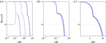
The characteristic equation (3.29) can be solved numerically by the Newton–Raphson method. Some results obtained in this way are shown for a few values of the parameters in figures 5 and 6 for
 ${\it\mu}_{l}={\it\mu}_{u}$
. Figure 5 shows graphs of
 $\text{Im}\,{\it\omega}/A$
versus
 $\mathit{Oh}$
for different values of
 ${\it\rho}_{u}/{\it\rho}_{l}$
and
 ${\it\Gamma}$
with
 $C_{\ast }=0$
. In figure 5(a)
 ${\it\rho}_{u}/{\it\rho}_{l}=1$
, while
 ${\it\Gamma}$
increases by two orders of magnitude from left to right. As
 $\mathit{Oh}\rightarrow 0$
(and
 $k\rightarrow 0$
),
 ${\it\omega}$
is purely imaginary with two roots tending to 1 and 0, respectively, in agreement with (3.35). As
 $\mathit{Oh}\rightarrow \infty$
(and
 $k\rightarrow \infty$
), on the other hand,
 $\text{Im}\,{\it\omega}$
becomes negative, corresponding to a stable interface. Thus, as expected, there is a range of sufficiently small wave numbers where the action of surface tension is insufficient to stabilize the interface. The point of discontinuity of the tangent in figure 5 (and later in figure 7) corresponds to the confluence of a pair of purely imaginary roots into a complex one so that, to the left of this point, the instability is monotonic while, to the right, it is oscillatory; in figure 5 we show both branches to the left of this point of discontinuity only for the smallest value of
 ${\it\Gamma}$
(dash-dot line) so as not to encumber the figures.
Dependence of
 $\text{Im}\,{\it\omega}/A$
on the Ohnesorge number
 $\mathit{Oh}$
for various values of
 ${\it\Gamma}$
and
 ${\it\rho}={\it\rho}_{u}/{\it\rho}_{l}$
with
 $C=0$
and
 ${\it\mu}_{u}/{\it\mu}_{l}=1$
. (a)
 ${\it\rho}=1$
and
 ${\it\Gamma}=2.83\times 10^{-4}$
(dash-dot),
 $2.83\times 10^{-3}$
(dash),
 $2.83\times 10^{-2}$
(solid); the confluence of the two branches shown for the leftmost curve occurs in all cases but has been omitted from the other curves in order not to encumber the figures. (b)
 ${\it\Gamma}=2.83\times 10^{-4}$
and
 ${\it\rho}=0.01$
(solid), 0.1 (dash), 1 (dash-dot). (c)
 ${\it\Gamma}=0.1$
and
 ${\it\rho}=0.01$
(solid), 0.1 (dash), 1 (dash-dot).

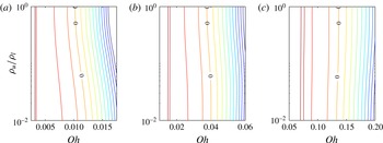
Contour plots of
 $\text{Im}\,{\it\omega}/A$
for
 $C=0$
and
 ${\it\mu}_{u}/{\it\mu}_{l}=1$
: (a)
 ${\it\Gamma}=2.83\times 10^{-4}$
; (b)
 ${\it\Gamma}=2.83\times 10^{-3}$
; (c)
 ${\it\Gamma}=2.83\times 10^{-2}$
. The interface is unstable, i.e.
 $\text{Im}\,{\it\omega}>0$
, to the left of the line marked 0 and stable to the right. The iso-lines are separated by equal increments of 0.2.

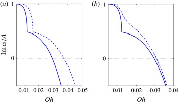
Illustration of the dependence of
 $\text{Im}\,{\it\omega}/A$
on the Ohnesorge number
 $\mathit{Oh}$
, viscosity and
 $C_{\ast }$
. (a)
 ${\it\rho}_{u}/{\it\rho}_{l}=1$
and
 $C_{\ast }=0$
; solid line,
 ${\it\mu}_{u}/{\it\mu}_{l}=0.5$
,
 ${\it\Gamma}=1.84\times 10^{-3}$
; dashed line,
 ${\it\mu}_{u}/{\it\mu}_{l}=1$
,
 ${\it\Gamma}=2.83\times 10^{-3}$
(same case as shown by the dashed line in figure 5
a); dash-dot line,
 ${\it\mu}_{u}/{\it\mu}_{l}=2$
,
 ${\it\Gamma}=5.20\times 10^{-3}$
. (b)
 ${\it\rho}_{u}/{\it\rho}_{l}=1$
,
 ${\it\mu}_{u}/{\it\mu}_{l}=0.5$
and
 ${\it\Gamma}=1.84\times 10^{-3}$
; solid line,
 $C_{\ast }=0$
; dash-dot line,
 $C_{\ast }=20$
.

These and some of the later figures show that the strongest instability is found to occur for
 $k\rightarrow 0$
. In considering this prediction one should not lose sight of the fact that ours is a local analysis. The geometry of every specific system will be able to accommodate only perturbations up to some maximum wavelength, and the predicted instability cannot occur if this natural cutoff length is shorter than the shortest unstable wavelength. We give a specific example of this argument in § 6 in the case of co-flowing jets.
The increase of the parameter
 ${\it\Gamma}$
can be interpreted as due to the increase of the velocity gradient
 $A$
, and is seen to increase the range of unstable wave numbers. Alternatively, increasing
 ${\it\Gamma}$
can be seen as a decrease of surface tension or an increase of viscosity, both of which also have a destabilizing effect, the former due to the decrease of the restoring force and the latter due to the increased amount of fluid dragged along by the interfacial perturbation. In figure 5(b)
 ${\it\Gamma}=2.83\times 10^{-4}$
and in figure 5(c)
 ${\it\Gamma}=0.1$
, while
 ${\it\rho}_{u}/{\it\rho}_{l}$
increases from 0.01 to 1. The effect of density is relatively small, corresponding to the small effect that inertia forces have in the situation considered, where viscosity and surface tension are dominant factors.
Figure 6(a)–(c) show lines of constant
 $\text{Im}\,{\it\omega}/A$
in the
 $(\mathit{Oh},{\it\rho})$
plane for values of
 ${\it\Gamma}$
spanning two orders of magnitude; the neutral stability curve
 $\text{Im}\,{\it\omega}=0$
is marked by zeros and the instability region is to the left of this curve. As noted above, for
 ${\it\mu}_{l}={\it\mu}_{u}$
as here, the results are symmetric upon interchange of
 ${\it\rho}_{u}$
and
 ${\it\rho}_{l}$
, so we only show the range
 $10^{-2}\leqslant {\it\rho}_{u}/{\it\rho}_{l}\leqslant 1$
. For small
 ${\it\Gamma}$
, i.e. essentially when viscous effects are small, increasing the density of one fluid is seen to have a stabilizing effect as the neutral curve moves toward smaller
 $\mathit{Oh}$
, i.e. toward longer waves or larger strain. The effect however reverses as
 ${\it\Gamma}$
is increased, reflecting the shift in the balance between the inertial and the viscous forces determining the instability.
Figures 7(a) and 7(b) show the effects of
 ${\it\mu}_{l}/{\it\mu}_{u}$
and
 $C_{\ast }$
on the imaginary part of the root of the characteristic equation (3.29) for
 ${\it\rho}_{u}/{\it\rho}_{l}=1$
. As noted earlier, in this case the results are invariant upon interchanging
 ${\it\mu}_{l}$
and
 ${\it\mu}_{u}$
. With
 $C_{\ast }=0$
, decreasing the viscosity of one fluid makes that fluid more mobile and increases the range of unstable wave numbers (figure 7
a). The two lines in figure 7(b) correspond to
 $C_{\ast }=0$
(solid) and
 $C_{\ast }=20$
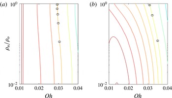
. Figure 8 is similar to figure 6 and compares the effect of the density ratio for these two values of
 $C_{\ast }$
.
Contour plots of
 $\text{Im}\,{\it\omega}/A$
for (a)
 $C_{\ast }=0$
and (b)
 $C_{\ast }=20$
with
 ${\it\rho}_{u}/{\it\rho}_{l}=1$
,
 ${\it\mu}_{u}/{\it\mu}_{l}=0.5$
,
 ${\it\Gamma}=1.84\times 10^{-3}$
. The interface is unstable, i.e.
 $\text{Im}\,{\it\omega}>0$
, to the left of the line marked 0 and stable to the right. The iso-lines are separated by equal increments of 0.2.

4. Numerical simulation
We now show the results of some numerical simulations of the two-dimensional problem, which provide a more complete picture of the phenomenon of interest here. A brief description of the numerical method is provided in appendix C.
The computational domain extends over the square
 $-L<x,y<L$
. The edges of the computational domain are far enough from the region where the disturbance develops that velocity boundary conditions corresponding to the undisturbed flow given by (3.5) and (3.6) can be used. To adhere as closely as possible to the linear framework, the convection terms in the Navier–Stokes equations are omitted at first. An example illustrating the significance of these terms is presented at the end of this section. In the analysis described in the previous section, we have also dropped terms responsible for the appearance of the variable
 $x$
in some of the boundary conditions of § 3.2. The corresponding physical effects – the continuity of the tangential velocity and stress – are however implicit in the mathematical model used in the computation and cannot be removed. In particular, the compression of the interface inherent in the kinematic condition (3.10) and (3.11) is present in the simulation, with consequences that will be commented upon later when we discuss the results of the simulations shown in figure 11.
In order to compare the numerical results with the local linear analysis of the previous section, we start by considering an initial perturbation of the form
 $$\begin{eqnarray}{\it\eta}(x,t=0)=\frac{1}{2}{\it\eta}_{0}\left(1+\tanh \frac{a^{2}-x^{2}/L^{2}}{d}\right)\cos kx,\end{eqnarray}$$
which localizes a sinusoidal perturbation near the origin, and focus on the time dependence of
 ${\it\eta}(x=0,t)$
. Two examples with
 ${\it\eta}_{0}=0.01L$
,
 $k_{\ast }=kL=30$
,
 ${\it\rho}_{l}={\it\rho}_{u}$
,
 ${\it\mu}_{l}={\it\mu}_{u}$
,
 ${\it\Gamma}=1$
are shown in figure 9 with
 $a=0.4$
,
 $d=0.04$
and only the parameter
 $A$
non-zero. The dimensional value of
 $k$
used in the definitions (3.37) and (3.39) is taken as
 $k_{\ast }/L$
. We show results for two cases with
 $\mathit{Re}=9$
,
 $\mathit{Ca}=3$
, and
 $\mathit{Re}=10^{-4}$
,
 $\mathit{Ca}=0.01$
, which are predicted by the linear theory to be unstable and stable, respectively.
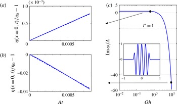
(a,b) Comparison between the analytical (dashed lines) and numerical (solid lines) interface perturbation amplitudes for an unstable (a) and stable case (b) with
 $\mathit{Oh}=0.577$
,
 $\mathit{Re}=9$
, and
 $\mathit{Oh}=10$
,
 $\mathit{Re}=10^{-4}$
, respectively. For both cases
 ${\it\Gamma}=1$
,
 ${\it\rho}_{u}/{\it\rho}_{l}=1$
and
 ${\it\mu}_{u}/{\it\mu}_{l}=1$
. (c) Graph of
 $\text{Im}\,{\it\omega}/A$
versus
 $\mathit{Oh}$
. The points corresponding to (a,b) are marked by black dots. The inset is a graph of the initial condition (4.1).

Figure 9(c) shows the ratio
 $\text{Im}\,{\it\omega}/A$
versus
 $\mathit{Oh}$
for
 ${\it\Gamma}=1$
; the inset is a graph of (4.1). Figure 9(a,b) shows
 ${\it\eta}(x=0,t)/{\it\eta}_{0}$
as calculated numerically and analytically corresponding to the two values of
 $\mathit{Oh}$
marked on the dispersion relation in figure 9(c). Here, as in the rest of this section, the non-dimensional time is defined as
 $\mathit{At}$
. Both the growth of the unstable case and the decay of the stable case are closely reproduced by the computation.
For the examples that follow, we take an initial interface shape given by
 $$\begin{eqnarray}{\it\eta}(x,t=0)={\it\eta}_{0}\exp \left(-{\textstyle \frac{1}{2}}k^{2}x^{2}\right),\end{eqnarray}$$
with
 ${\it\eta}_{0}/L=0.1$
and
 $k_{\ast }=kL=30$
, and vary the numerical values of the parameters
 $A,B,C$
and
 $D$
of the base flow. In presenting the results we use the same definitions of
 $\mathit{Ca}$
,
 $\mathit{Re}$
and
 $\mathit{We}$
as given in (3.37) and (3.39), replacing
 $k$
by
 $k_{\ast }/L$
.
We start with an example in which only
 $A$
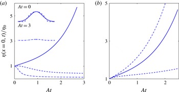
is non-zero and positive, which is already sufficient to capture the essence of the instability. Figure 10(a) shows the time evolution of the perturbation amplitude for fluids of equal density and viscosity,
 ${\it\rho}_{u}/{\it\rho}_{l}=1$
, and
 ${\it\mu}_{u}/{\it\mu}_{l}=1$
; the three lines are for
 $\mathit{Ca}=0.1$
, 0.4 and 1, all with
 $\mathit{Re}=1$
. The corresponding values of
 $\mathit{Oh}$
and
 ${\it\Gamma}$
are
 $\mathit{Oh}=0.316$
,
 ${\it\Gamma}=0.1$
;
 $\mathit{Oh}=0.632$
,
 ${\it\Gamma}=0.4$
;
 $\mathit{Oh}=1$
,
 ${\it\Gamma}=1$
. The stabilizing effect of surface tension is smallest for
 $\mathit{Ca}=1$
, and the disturbance grows. For
 $\mathit{Ca}=0.4$
, there is an initial growth followed by convergence to a steady state with an amplitude smaller than the initial one. We see here an important effect not captured by the linear stability analysis of the previous section, namely that, as the initial disturbance grows, the curvature at the tip increases, thus strengthening the restoring effect of surface tension. Thus, even in the strongly unstable case
 $\mathit{Ca}=1$
, upon close examination it is seen that the initial growth slows down before picking up again. For
 $\mathit{Ca}=0.1$
the initial growth is absent, and for large times the interface shape converges to a steady configuration with an amplitude smaller than for
 $\mathit{Ca}=0.4$
. For this last case we also tested the effect of the initial condition using, in addition to (4.2), also
 ${\it\eta}(x,0)={\it\eta}_{0}[1-3.832(x/L)^{2}]$
for
 $|x/L|\leqslant 1.958$
and
 ${\it\eta}(x,0)=0$
otherwise; the numerical parameters have been adjusted so that the area under the curves
 ${\it\eta}(x,0)$
is the same in both cases. The two initial shapes are shown in the top inset of the figure but their subsequent evolution is indistinguishable, as can be seen from the lower inset.
Time evolution of
 ${\it\eta}(0,t)/{\it\eta}_{0}$
with
 $\mathit{Re}=1$
and
 ${\it\rho}_{u}/{\it\rho}_{l}=1$
. (a)
 $\mathit{Ca}=0.1$
(dotted line),
 $\mathit{Ca}=0.4$
(dashed line) and
 $\mathit{Ca}=1$
(solid line), all for
 ${\it\mu}_{u}/{\it\mu}_{l}=1$
. The inset shows two initial configurations and the interface shape at
 $\mathit{At}=3$
, where the two results are indistinguishable, for
 $\mathit{Ca}=0.1$
; see text. (b) As in (a) with
 $\mathit{Ca}=1$
and
 ${\it\mu}=1/3$
(dashed line),
 ${\it\mu}=1$
(solid line), and
 ${\it\mu}=3$
(dash-dot line).

Figure 10(b) shows the effect of the viscosity ratio,
 ${\it\mu}_{u}/{\it\mu}_{l}=3$
(dash-dot line), 1 (solid line) and
 $1/3$
(dashed line), for
 $\mathit{Ca}=1$
and equal densities as before. The initial perturbation is directed into the upper fluid, but the results are also applicable to the downward directed case by simply switching the viscosity ratios. It is seen that growth is strongest when the perturbation is initially directed into the higher-viscosity fluid. This is a general result that we have encountered in all our simulations, irrespective of the density ratio.
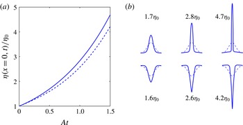
(a) Time evolution of
 ${\it\eta}(0,t)/{\it\eta}_{0}$
with
 $\mathit{Re}=10$
,
 $\mathit{Ca}=10$
,
 ${\it\rho}_{u}/{\it\rho}_{l}=0.5$
and
 ${\it\mu}_{u}/{\it\mu}_{l}=9$
. The solid and dashed lines are for initially upward or downward oriented perturbation, respectively. (b) Three snapshots of the interface configuration at
 $\mathit{At}=0.5$
, 1.0 and 1.5: top row, upward bump; bottom row, downward bump.

Figure 11(a) refers to a lighter, but more viscous, upper fluid,
 ${\it\rho}_{u}/{\it\rho}_{l}=0.5$
,
 ${\it\mu}_{u}/{\it\mu}_{l}=9$
, for
 $\mathit{Ca}=10$
(i.e.
 $\mathit{Oh}=1$
,
 ${\it\Gamma}=3.16$
) and upward- and downward-directed initial perturbations. Snapshots of the interface at the beginning (dashed line) and end of the computation are shown in figure 11(b). The destabilizing effect of the larger viscosity of the fluid into which the interface disturbance is initially directed is manifest in these graphs.
The analysis of § 3 predicts that the growth rate of the instability increases with the wavelength of the perturbation, which would lead one to expect a broadening of the initial perturbation, which is not observed in the interface shapes of figure 11(b) and the figures that follow. The reason is the compressive effect of the base flow, which is not present in the analysis due to the neglect of the right-hand side of (3.11), while it is implicit in the mathematical model used in the simulation, as already noted at the beginning of this section.
It will be recalled from § 3.1 that the main effect of the parameter
 $B$
on the base flow is to tilt the dividing line between the converging streams away from the vertical. However, it was shown in the previous section that the linear stability analysis is independent of
 $B$
. Thus, it may be expected that this parameter will not introduce major differences in the results. This expectation is confirmed in figure 12, in which
 $B=-3A/L$
,
 $\mathit{Re}=10$
,
 $\mathit{Ca}=10$
(i.e.
 $\mathit{Oh}=1$
,
 ${\it\Gamma}=3.16$
),
 ${\it\rho}_{u}/{\it\rho}_{l}=0.5$
and
 ${\it\mu}_{u}/{\it\mu}_{l}=3$
. The two panels of this figure refer to initial perturbations directed into the upper and lower fluids, and the lines show the initial perturbation at
 $t=0$
and at two later times. The insets place the last calculated shape in the context of the streamlines of the undisturbed flow. The perturbation is seen to bend to the left as it grows, closely following the direction of the dividing line of the unperturbed flow.
Snapshots of the surface shape at times
 $\mathit{At}=0$
, 0.5 and 1 for
 $B=-3A/L$
,
 $\mathit{Re}=10$
,
 $\mathit{Ca}=10$
,
 ${\it\rho}_{u}/{\it\rho}_{l}=0.5$
and
 ${\it\mu}_{u}/{\it\mu}_{l}=3$
. The insets show the last surface shape against the background of the streamlines of the undisturbed flow. (a) Upward surface perturbation; (b) downward surface perturbation.

A non-zero value of the parameter
 $C$
introduces a second stagnation point at
 $x=2A/C$
where vorticity does not vanish. For
 $D=0$
there are closed streamlines in the upper half-plane for
 $BC>0$
and in the lower half-plane for
 $|{\it\mu}B/[3({\it\mu}-1)]|<|C|$
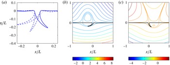
; when these inequalities are not satisfied, the streamlines are open. The case in which closed streamlines are present in both fluids is reminiscent of the situation encountered in the translation of a drop in an immiscible liquid (cf. figure 23); figures 13(c) and 14(c) illustrate examples of this situation.
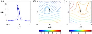
(a) Snapshots of the surface shape for an initially upward-oriented perturbation at
 $t=0$
(dotted line) and
 $\mathit{At}=1.0$
for
 $B=-3A/L$
,
 $\mathit{Re}=10$
,
 $\mathit{Ca}=10$
,
 ${\it\rho}_{u}/{\it\rho}_{l}=0.5$
, and
 ${\it\mu}_{u}/{\it\mu}_{l}=3$
. The three results for
 $C=0$
and
 $C=\pm 4A/L$
are barely distinguishable. (b) Last surface shape against the background of the streamlines of the undisturbed flow for
 $C=-4A/L$
. (c) Last surface shape against the background of the streamlines of the undisturbed flow for
 $C=4A/L$
.

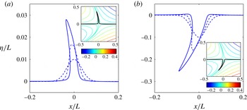
(a) Snapshots of the surface shape for an initially downward-oriented perturbation at
 $t=0$
(dotted line) and
 $\mathit{At}=1.0$
for
 $B=-3A/L$
,
 $\mathit{Re}=10$
,
 $\mathit{Ca}=10$
,
 ${\it\rho}_{u}/{\it\rho}_{l}=0.5$
, and
 ${\it\mu}_{u}/{\it\mu}_{l}=3$
. The dashed line is for
 $C=0$
, the dash-dot line for
 $C=-4A/L$
, and the solid line for
 $C=4A/L$
. (b) Last surface shape against the background of the streamlines of the undisturbed flow for
 $C=-4A/L$
. (c) Last surface shape against the background of the streamlines of the undisturbed flow for
 $C=4A/L$
.

Figure 13 shows results for
 ${\it\mu}_{u}/{\it\mu}_{l}=3$
,
 $B=-3A/L$
and
 $C=\pm 4A/L$
with an initially upward surface perturbation. The shape of the interface at the last computed time is shown in figure 13(a), and set against the undisturbed flow pattern for
 $C=-4A/L$
in figure 13(b) and against the undisturbed flow pattern for
 $C=4A/L$
and in figure 13(c). In both cases the perturbation exhibits a strong tendency to grow along the streamlines which separate the opposite incoming streams with a very small effect of the parameter
 $C$
. The additional stagnation points are at
 $x=\pm L/2$
, and apparently they are too far to have a significant influence on the development of the perturbation, which is dominated by
 $A$
and
 $B$
. The same tendency to follow the separatrix streamline is found when the initial perturbation is downward (see figure 14), to the left for
 $C=-4A/L$
and to the right for
 $C=4A/L$
.
As
 $|D|$
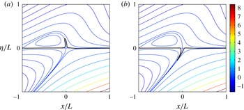
increases there is a tendency for closed streamlines to become open, as can be seen by comparing the streamline patterns of figure 15, for which
 $D=3A/L$
, with those of figure 14(c), in which the parameters have the same values except that
 $D=0$
. Qualitatively, the effect on the development of the perturbation is similar to that shown in figures 13 and 14, with the perturbation growing along the separatrix streamline as shown in the examples of figure 15.
Snapshots of the interface shape for
 $B=-3A/L$
,
 $C=-2A/L$
,
 $D=3A/L$
,
 $\mathit{Re}=10$
,
 $\mathit{Ca}=10$
,
 ${\it\rho}_{u}/{\it\rho}_{l}=0.5$
, and
 ${\it\mu}_{u}/{\it\mu}_{l}=3$
. (a) Initially upward perturbation at
 $\mathit{At}=1.0$
; (b) initially downward surface shape at
 $\mathit{At}=0.66$
. The streamlines in the background show the unperturbed flow.

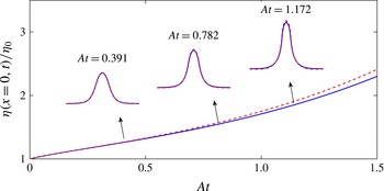
As a final point, since both the analysis and the simulations described thus far were conducted omitting convective effects, it is interesting to examine the significance of this approximation in at least one case. Some numerical results comparing the interface evolution with and without convection are shown in figure 16. This is the same as the cases
 $\mathit{Ca}=1$
of figure 10, i.e. only
 $A$
is non-zero,
 ${\it\rho}_{u}/{\it\rho}_{l}=1$
,
 ${\it\mu}_{u}/{\it\mu}_{l}=1$
and
 $\mathit{Re}=1$
, (i.e.
 $\mathit{Oh}=1$
,
 ${\it\Gamma}=1$
); the initial perturbation is given by (4.2) with
 ${\it\eta}_{0}=0.1$
and
 $\partial {\it\eta}/\partial t=0$
. It is seen here that convection is not a very significant effect compared with the compression of the interface and the non-linearity induced by the severe distortion of the interface. Of course, this conclusion will depend on the Reynolds number which, however, is usually not large when capillarity and viscosity are both significant, as in the examples shown in figure 1, among others.
Time evolution of
 ${\it\eta}(0,t)/{\it\eta}_{0}$
with non-zero
 $A$
,
 $\mathit{Re}=1$
,
 $\mathit{Ca}=1$
,
 ${\it\rho}_{u}/{\it\rho}_{l}=1$
, and
 ${\it\mu}_{u}/{\it\mu}_{l}=1$
. Solid lines, without convection effects; dashed lines, with convection effects. The corresponding interface shapes at
 $\mathit{At}=0.391$
,
 $\mathit{At}=0.782$
, and
 $\mathit{At}=1.172$
are also compared.

5. Surfactant effects
As a consequence of the flow directed toward the zero-vorticity point, a surface-active substance on the interface will tend to accumulate there. Since surface tension is the only force opposing the instability, the weakening of its action caused by the surfactant will have a destabilizing action. It is therefore of interest to show some numerical simulations demonstrating this effect.
We model the transport of the surfactant by the equation (see e.g. Stone Reference Stone1990)
 $$\begin{eqnarray}\frac{\partial {\it\Phi}}{\partial t}+\boldsymbol{{\rm\nabla}}_{s}\boldsymbol{\cdot }({\it\Phi}\boldsymbol{u}_{s})+(\boldsymbol{{\rm\nabla}}_{s}\boldsymbol{\cdot }\boldsymbol{n})(\boldsymbol{u}\boldsymbol{\cdot }\boldsymbol{n}){\it\Phi}=\frac{1}{\mathit{Pe}}{\rm\nabla}_{s}^{2}{\it\Phi}+\mathit{Bi}(1+k_{ad})\left(1-\frac{{\it\Phi}}{{\it\Phi}_{eq}}\right).\end{eqnarray}$$
Here
 ${\it\Phi}$
stands for the surfactant concentration normalized by the maximum possible value corresponding to a closely packed molecular arrangement, and
 ${\it\Phi}_{eq}$
is the normalized surfactant concentration in equilibrium with the bulk concentration in the liquid;
 $\boldsymbol{u}_{s}$
is the velocity tangent to the surface,
 $\boldsymbol{{\rm\nabla}}_{s}$
and
 ${\rm\nabla}_{s}^{2}$
are the surface divergence and Laplace operators and
 $\mathit{Pe}$
is the Péclet number. The last term on the right-hand side is a simple model of adsorption–desorption effects. The Biot number,
 $\mathit{Bi}$
, is the ratio of the characteristic desorption rate to the surface convection time scale
 $A$
. The adsorption parameter
 $k_{ad}$
is the product of the adsorption rate by the bulk-liquid concentration divided by the desorption rate (see e.g. Eggleton & Stebe Reference Eggleton and Stebe1998). The non-dimensional time is given by
 $\mathit{At}$
as before. We assume that surface tension depends on
 ${\it\Phi}$
according to
 $$\begin{eqnarray}\frac{{\it\sigma}}{{\it\sigma}_{0}}=1+{\it\zeta}\log \frac{1-{\it\Phi}}{1-{\it\Phi}_{eq}},\end{eqnarray}$$
where
 ${\it\zeta}$
is the elasticity number (see e.g. Eggleton & Stebe Reference Eggleton and Stebe1998);
 ${\it\sigma}_{0}$
is the value of the surface tension coefficient when
 ${\it\Phi}={\it\Phi}_{eq}$
. The calculations are started with the constant equilibrium value
 ${\it\Phi}={\it\Phi}_{eq}$
on the entire interface and the same initial shape (4.2) used earlier. The same non-dimensional parameters used earlier are used here, with
 ${\it\sigma}_{0}$
replacing
 ${\it\sigma}$
in the definitions (3.37) of
 $\mathit{Ca}$
and
 ${\it\Gamma}$
; we take
 ${\it\rho}_{l}={\it\rho}_{u}$
,
 ${\it\mu}_{l}={\it\mu}_{u}$
,
 $\mathit{Ca}=0.4$
and
 $\mathit{Re}=1$
(
 ${\it\Gamma}=0.4$
,
 $\mathit{Oh}=0.632$
,
 $\mathit{We}=0.4$
); only the parameter
 $A$
is non-zero in the examples of this section.
Our first example is with
 $\mathit{Bi}=0$
, i.e. with the neglect of adsorption–desorption effects, and
 ${\it\zeta}=0.5$
,
 ${\it\Phi}_{eq}=0.5$
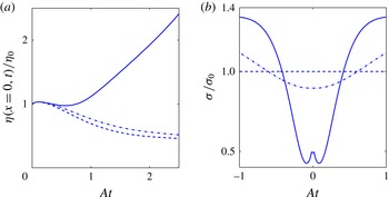
. Figure 17(a) compares the evolution of
 ${\it\eta}(x=0,t)/{\it\eta}_{0}$
for
 $\mathit{Pe}=0$
, 0.1 and 1 while figure 17(b) shows the distribution of the dimensionless surface tension coefficient (5.2) over the interface at the time
 $\mathit{At}=2.5$
. For
 $\mathit{Pe}=0$
, the surfactant diffusivity is very large and, accordingly, the surface tension, shown by the dashed line in figure 17(b), remains constant. The amplitude of the interfacial disturbance saturates to a constant value, as found earlier for the stable constant-surface-tension cases. A similar saturation takes place for
 $\mathit{Pe}=0.1$
(dash-dot line), although the final amplitude is somewhat larger than for
 $\mathit{Pe}=0$
. For this value of
 $\mathit{Pe}$
the surface tension coefficient is somewhat affected by convection, resulting in a smaller value near the stagnation region and a larger value elsewhere. When
 $\mathit{Pe}=1$
(solid line), all other parameters being equal, the stability threshold is exceeded and the amplitude grows. The surface tension is greatly reduced. The small local maximum near the apex of the perturbation is due to the relatively small convection in the immediate neighbourhood of
 $x=0$
(cf. (3.5) and (3.6)).
Effects of an insoluble surfactant (
 $\mathit{Bi}=0$
) for
 $\mathit{Pe}=0$
(dashed lines),
 $\mathit{Pe}=1$
(dash-dot lines) and
 $\mathit{Pe}=10$
(solid lines) with
 $\mathit{Re}=1$
,
 $\mathit{Ca}=0.4$
,
 ${\it\Gamma}=0.4$
,
 $\mathit{We}=0.4$
,
 ${\it\rho}_{u}/{\it\rho}_{l}=1$
,
 ${\it\mu}_{u}/{\it\mu}_{l}=1$
,
 ${\it\Phi}_{eq}=0.5$
. (a) Time evolution of
 ${\it\eta}(x=0,t)/{\it\eta}_{0}$
; (b) dimensionless surface tension coefficient at
 $\mathit{At}=2.5$
.

The effects of adsorption and desorption are illustrated in figure 18, in which we take
 $\mathit{Pe}\rightarrow \infty$
,
 $k_{ad}=0.33$
and, in descending order,
 $\mathit{Bi}=0$
, 0.1, 0.5 and 10; here
 ${\it\zeta}=0.25$
and
 ${\it\Phi}_{eq}=0.25$
. Figure 18(a) is the time dependence of the surface disturbance and figure 18(b) is the time dependence of the dimensionless surface tension coefficient at
 $x=0$
. When
 $\mathit{Bi}=0$
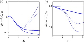
(dashed line), the surfactant does not diffuse into the surrounding liquid but remains on the interface. Initially, the surface tension is large enough to stabilize the interface due to the increasing curvature but, as the surfactant accumulates in the neighbourhood of the stagnation point, the local surface tension decreases and is unable to oppose the destabilizing action of the flow. As
 $\mathit{Bi}$
increases, desorption becomes possible as the surfactant accumulates. The growth rate of the disturbance starts to decrease and it eventually reverses, with a stable long-time configuration with an amplitude smaller than the initial one. The surface tension coefficient at
 $x=0$
, shown in figure 18(b), demonstrates the progressive depletion of the surfactant as
 $\mathit{Bi}$
increases.
Effects of a soluble surfactant with
 $\mathit{Pe}\rightarrow \infty$
,
 $k_{ad}=0.33$
and
 $\mathit{Bi}=0$
(dashed lines), 0.1 (dash-dot lines), 0.5 (solid lines with marks) and 10 (solid lines); here
 $\mathit{Ca}=0.4$
,
 $\mathit{Re}=1$
,
 ${\it\zeta}=0.25$
and
 ${\it\Phi}_{eq}=0.25$
. (a) Time evolution of
 ${\it\eta}(x=0,t)/{\it\eta}_{0}$
; (b) time evolution of the surface tension coefficient at
 $x=0$
.

6. Two actual flow examples
In conclusion it is of some interest to show how the local flow structures studied so far play in specific flows. For this purpose we consider two two-dimensional examples: a coaxial jet and a liquid drop rising by buoyancy. In both cases the liquids are immiscible.
Suryo & Basaran (Reference Suryo and Basaran2006) studied the axisymmetric drop formation from an inner liquid stream in a co-flowing outer fluid in the Stokes-flow regime. They parametrized their results in terms of the viscosity ratio
 ${\it\mu}={\it\mu}_{i}/{\it\mu}_{o}$
and of the ratio
 $Q_{r}=Q_{o}/Q_{i}$
of the outer stream flow rate
 $Q_{o}$
to the inner stream flow rate
 $Q_{i}$
. They found that in all cases inner fluid drops detach from a thin ligament and the drop size decreases with increasing
 $Q_{r}$
. As
 $Q_{r}$
increases, however, there is a marked qualitative change, with the base of the ligament turning from convex toward the outer fluid to concave and nearly cusp-like, with a corresponding qualitative change in the process of drop formation (see figure 3 in Suryo & Basaran Reference Suryo and Basaran2006). Corresponding to the transition to the near-cuspidal shape which, for
 ${\it\mu}_{o}={\it\mu}_{i}$
, occurred at about
 $Q_{r}=10$
, the ligament became significantly longer and thinner with a correspondingly dramatic decrease in the size of the detaching drops (see figure 1
c). We have carried out simulations of this process for the two-dimensional, rather than axisymmetric, case. Initially the free surface is taken to be flat at the outlet of the inner duct. The inflow velocity fields for the inner and outer ducts are parabolic and are made to gradually increase with time until the desired steady state value is reached at a dimensionless time
 $U_{i}t/d_{i}\simeq 0.067$
. Here
 $U_{i}$
is the mean velocity of the inner liquid, taken as reference velocity, and
 $d_{i}$
is the diameter (width) of the inner duct, taken as reference length; indices
 $i$
and
 $o$
refer to the inner and outer fluids, respectively. The total width of the computational domain is
 $d_{o}/d_{i}=2$
and the length is
 $8d_{i}$
. The thickness of the inner duct wall is negligible and no-slip conditions are applied on all solid surfaces. The interface is held pinned at the exit of the inner duct. The fluids have equal densities, while
 ${\it\mu}_{i}/{\it\mu}_{o}=0.25$
and the Reynolds and capillary numbers of the inner fluid are
 $\mathit{Re}_{i}=d_{i}U_{i}/{\it\nu}_{i}=0.0667$
and
 $\mathit{Ca}_{i}=U_{i}{\it\mu}_{i}/{\it\sigma}=0.00667$
.
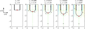
We consider two cases in detail. In the first one
 $Q_{r}=U_{o}/U_{i}=2$
, while the outer Reynolds and capillary numbers are
 $\mathit{Re}_{o}=(d_{o}-d_{i})U_{o}/{\it\nu}_{o}\simeq 0.133$
and
 $\mathit{Ca}_{o}=U_{o}{\it\mu}_{o}/{\it\sigma}\simeq 0.533$
. For the second case,
 $Q_{r}=U_{o}/U_{i}=60$
,
 $\mathit{Re}_{o}\simeq 7$
and
 $\mathit{Ca}_{o}\simeq 16$
. The results are shown in figures 19 and 20; the dimensionless time is defined as
 $t_{\ast }=U_{i}t/d_{i}$
and
 $d_{i}$
is used to non-dimensionalize the curvature
 ${\it\kappa}$
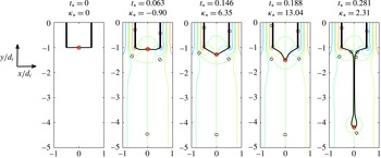
on the axis (plane) of symmetry. The figures show the interface by the solid black line and several iso-vorticity lines at successive instants of time. In the right half of the flow, the outer-fluid vorticity is positive near the outer wall and negative near the inner wall, which causes the appearance of a zero-vorticity line terminating in the outer fluid on the axis of symmetry; the situation in the left half is the mirror image. Another zero-vorticity line, due to the symmetry of the flow, runs along the axis of symmetry and crosses the interface between the two liquids. This is therefore a zero-vorticity surface point where the instability studied in this paper can set in under suitable conditions.
Stable two-dimensional coaxial flow with
 $U_{o}/U_{i}=2$
: snapshots of the interface with a few iso-vorticity contours at several instants. The red circle marks the position of the zero-vorticity point on the interface. Here
 ${\it\rho}_{i}/{\it\rho}_{o}=1$
,
 ${\it\mu}_{i}/{\it\mu}_{o}=0.25$
,
 $\mathit{Re}_{i}=d_{i}U_{i}/{\it\nu}_{i}\simeq 0.667$
,
 $\mathit{Ca}_{i}=U_{i}{\it\mu}_{i}/{\it\sigma}\simeq 0.00667$
,
 $\mathit{Re}_{o}=(d_{o}-d_{i})U_{o}/{\it\nu}_{o}\simeq 0.133$
,
 $\mathit{Ca}_{o}=U_{o}{\it\mu}_{o}/{\it\sigma}\simeq 0.533$
;
 ${\it\kappa}_{\ast }={\it\kappa}d_{i}$
is the dimensionless curvature of the interface on the axis (plane) of symmetry.

Unstable two-dimensional coaxial flow with
 $U_{o}/U_{i}=60$
: snapshots of the interface with a few iso-vorticity contours at several instants. The red circle marks the position of the zero-vorticity point on the interface. Here
 ${\it\rho}_{i}/{\it\rho}_{o}=1$
,
 ${\it\mu}_{i}/{\it\mu}_{o}=0.25$
,
 $\mathit{Re}_{i}=d_{i}U_{i}/{\it\nu}_{i}\simeq 0.667$
,
 $\mathit{Ca}_{i}=U_{i}{\it\mu}_{i}/{\it\sigma}\simeq 0.00667$
,
 $\mathit{Re}_{o}=(d_{o}-d_{i})U_{o}/{\it\nu}_{o}\simeq 7$
,
 $\mathit{Ca}_{o}=U_{o}{\it\mu}_{o}/{\it\sigma}\simeq 16$
;
 ${\it\kappa}_{\ast }={\it\kappa}d_{i}$
is the dimensionless curvature of the interface on the axis (plane) of symmetry.

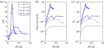
Figure 21(a) and (b) show the time evolution of the dimensionless curvature
 ${\it\kappa}d_{i}$
and interface velocity
 $V(x=0,t)/U_{i}$
for
 $Q_{r}=2,10,20$
and 60. The negative of the slope of the tangential velocity of the interface on the axis of symmetry is the parameter
 $A$
used in the analysis of § 3.1; the dimensionless value
 $Ad_{i}/U_{i}$
of this parameter is shown in figure 21(c) as a function of time for the same values of the velocity ratio; the other parameters
 $B$
etc. introduced in § 3.1 all vanish for this flow.
Time evolution of various interface quantities evaluated on the axis (plane) of symmetry for the coaxial jet problem with
 $U_{o}/U_{i}=2,10,20$
and 60. (a) Dimensionless interface curvature
 ${\it\kappa}d_{i}$
; (b) dimensionless interface velocity
 $V(x=0,t)/U_{i}$
; (c) dimensionless parameter
 $Ad_{i}/U_{i}$
characterizing the velocity gradient as defined in § 3.1.

Figures 19 and 21(a) show that the curvature of the interface in the case
 $Q_{o}/Q_{i}=2$
mildly increases to about 1.2, after which it starts to decreases due to the bulging out of the inner fluid drop; similar behaviour can be seen in figure 21(a) for
 $Q_{o}/Q_{i}=10$
. The interface behaviour for the high-velocity-ratio cases is quite different. Figure 20 shows the formation of a characteristic near-cusp with a very high curvature (see also figure 21
a). A long filament issues from this cusp, ultimately developing a small drop. These distinct behaviours are qualitatively the same as those reported by Suryo & Basaran (Reference Suryo and Basaran2006). In the highest-velocity case
 $Q_{r}=60$
, initially the stagnation pressure on the axis is so strong as to push the inner fluid back into the tube causing a negative curvature, which however becomes positive as more inner fluid is injected.
Although the time dependence of the flow and the progressively increasing curvature of the interface prevent a precise comparison with the results of the analysis of § 3, it is nonetheless interesting to show the predictions of that analysis for the growth rate versus the wave number for some values of the parameter
 $A_{\ast }$
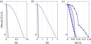
occurring in these simulations. Figure 22(a) shows the dimensionless growth rate
 $\text{Im}\,{\it\omega}d_{i}/U_{i}$
versus
 $kd_{i}$
at an early time,
 $t_{\ast }=0.012$
, when the curvature of the interface for the two cases of figures 19 and 20 is very small. In figure 22(b) the predictions of the analysis for the two cases are compared when the interface has reached the same curvature,
 ${\it\kappa}d_{i}\simeq 1.26$
, which is the maximum curvature of the low-velocity-ratio case; of course, this value of the curvature is reached at different times, as can be seen in figure 21(a). The values of
 $A$
in the small
 $Q_{r}$
and large
 $Q_{r}$
cases are quite different and so are the corresponding values of
 $\text{Im}\,{\it\omega}d_{i}/U_{i}$
. Replotting the same data as
 $(\text{Im}\,{\it\omega}d_{i}/U_{i})/A_{\ast }$
versus
 $kd_{i}/A_{\ast }$
does not result in a precise scaling but considerably reduces the difference between the curves as shown in figure 22(c). It can be seen here that, except for the smallest value
 $A_{\ast }=0.47$
, the wave number
 $k_{0}$
corresponding to a transition from unstable to stable behaviour is approximately
 $k_{0}d_{i}\sim 0.07A_{\ast }$
, corresponding to a perturbation wavelength
 ${\it\lambda}_{0}/d_{i}\sim 2{\rm\pi}/(0.07A_{\ast })\sim 70/A_{\ast }$
. The maximum value of
 $A_{\ast }$
for
 $Q_{r}=2$
is about 3.3, so
 ${\it\lambda}_{0}/d_{i}$
would equal approximately 20. The analogous estimate for
 $A_{\ast }=0.47$
would give
 ${\it\lambda}_{0}/d_{i}\sim 8.2$
. Clearly the size of the inner tube is not sufficient to accommodate unstable wavelengths, and the instability object of this paper cannot develop. For
 $Q_{r}=60$
, on the other hand, the value reached at the early time
 $U_{i}t/d_{i}=0.111$
(figure 21) is already about 52 and strongly increases at later times, so unstable wavelengths are possible in this case and the instability can develop, as indeed is found in the simulations of figure 20. Thus the theory predicts a range of unstable perturbations, the wavelength of which can be accommodated on the interface in the high-velocity case but not in the low-velocity one. As
 $A_{\ast }$
increases, shorter and shorter wavelengths become unstable and, correspondingly, the curvature of the jet tip increases. Figure 21(b) shows that the velocity of the jet tip also increases, in qualitative agreement with the theory of § 3 according to which
 $\text{Im}\,{\it\omega}$
is predicted to increase with
 $A$
, as can be seen in figure 5, for example. The result is the striking difference in the evolution of the interface, qualitatively similar to that found by Suryo & Basaran (Reference Suryo and Basaran2006).
Dimensionless solutions
 $\text{Im}\,{\it\omega}d_{i}/U_{i}$
of the characteristic equation (3.29) as functions of the dimensionless wave number
 $k_{\ast }=kd_{i}$
. (a)
 $Q_{r}=2$
with
 $A_{\ast }=0.47$
(solid line) and
 $Q_{r}=60$
with
 $A_{\ast }=12.01$
(dashed line) at
 $U_{i}t/d_{i}=0.012$
. (b) As in (a), at the instant when
 ${\it\kappa}_{\ast }={\it\kappa}d_{i}\simeq 1.26$
:
 $Q_{r}=2$
at
 $U_{i}t/d_{i}=0.313$
with
 $A_{\ast }=3.31$
(solid line), and
 $Q_{r}=60$
at
 $U_{i}t/d_{i}=0.111$
with
 $A_{\ast }=51.66$
(dashed line). (c) The same data as in (a) and (b) replotted in the form
 $(\text{Im}\,{\it\omega}d_{i}/U_{i})/A_{\ast }$
versus
 $k_{\ast }$
, for
 $A_{\ast }=0.47$
(line with triangles),
 $A_{\ast }=3.31$
(solid line),
 $A_{\ast }=12.01$
(dashed line) and
 $A_{\ast }=51.66$
(dash-dot line); results for the large value
 $A_{\ast }=200$
are also included to show the trend with increasing
 $A_{\ast }$
(line with circles).

As a second example, we consider a two-dimensional drop rising in a channel of diameter (width)
 $d_{c}$
. Initially the drop is an ellipse with a horizontal major axis, aspect ratio 0.6944 and area
 $({\rm\pi}/4)d_{d}^{2}$
, with
 $d_{d}=d_{c}/4$
centred at
 $y/d_{d}=-2$
. We also take
 ${\it\rho}_{d}/{\it\rho}_{o}=0.5$
,
 ${\it\mu}_{d}/{\it\mu}_{o}=0.1$
, with the index
 $d$
denoting the drop liquid and the index
 $o$
the host liquid. The Galilei number
 $\mathit{Ga}={\it\rho}_{o}\sqrt{gd_{d}^{3}(1-{\it\rho}_{d}/{\it\rho}_{o})}/{\it\mu}_{o}$
, where
 $g$
is the acceleration of gravity, equals 15.65. To limit the height of the computational domain, an inflow through the upper boundary with a Reynolds number
 $\mathit{Re}_{d}={\it\rho}_{o}d_{d}U_{in}/{\it\mu}_{o}$
equal to 5 is prescribed; outflow conditions are applied at the bottom of the computational domain, the height of which is
 $2d_{c}$
, while no-slip conditions are applied on the lateral boundaries; the dimensionless time is defined as
 $t_{\ast }=t\sqrt{g/d_{d}}$
.
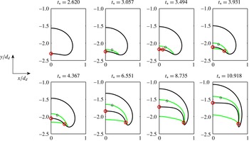
Initially the flow remains attached to the drop surface and the vorticity is negative throughout the right half of the drop shown in figure 23 (and positive in the other half, not shown). These two oppositely circulating regions generate a zero-vorticity point (red circle) at the position where the rear surface of the drop meets the axis (plane) of symmetry (the analogous point on the upper surface is not marked). With passing time the flow separates behind the drop and a recirculating region with negative vorticity forms there. Because of the continuity of velocity and tangential stress, this negative vorticity in the separation bubble causes the appearance of a positive vorticity near the back of the drop, while vorticity in the bulk of the drop remains negative to match the outer flow. Thus, inside the drop, a zero-vorticity line ending on the surface is generated. This line, which is shown in green in figure 23, is connected to a similar zero vorticity line in the liquid outside the drop. The zero-vorticity points on the surface are shown by red circles. The picture shown in figure 23 is not very precise, as the circulation behind the drop is very weak and the accuracy of the interpolation not very accurate. The difficulty is particularly acute at early times (first line of the figure), when the circulation just outside the drop is too weak to show and the position of the second zero-vorticity point cannot be established with good accuracy. The qualitative nature of this flow is nevertheless clear. In the neighbourhood of the point of intersection of the zero-vorticity lines with the interface, the flow is directed toward this point, which therefore is potentially subject to the instability studied in this paper. Indeed, as time passes, the interface develops an elongated structure in the neighbourhood of this point which eventually evolves into a skirt.
Two-dimensional liquid drop rising in an immiscible liquid: snapshots of the interface with the iso-vorticity lines
 ${\it\omega}=0$
, shown in grey (green online), at several instants; the circles (red online) indicate the approximate position of zero-vorticity points on the rear surface of the drop. Here
 ${\it\rho}_{d}/{\it\rho}_{o}=0.5$
and
 ${\it\mu}_{d}/{\it\mu}_{o}=0.1$
.

7. Summary and conclusions
Motivated by the similarities among several flows involving immiscible fluids in which small liquid masses detach from one of the fluids, some examples of which are shown in figure 1, we have attempted to develop a general understanding of processes of this type. Our results may be of interest in microfluidic applications, where situations of the type considered are frequently encountered, and may explain the mechanism by which very small oil drops in the ocean may detach from much larger oil masses.
Our analysis has centred on the flow in the neighbourhood of points (or lines) where the vorticity tangent to the interface vanishes. The flow can either converge or diverge toward such points on the two sides of the interface. In the former case, if strong enough, the associated compression of the interface can overcome the restraining effect of surface tension and lead to an instability by the mechanism sketched in figure 2. The effect is particularly strong in the presence of surfactants, which are swept by the flow toward the zero-vorticity point. We have carried out a linear stability analysis of the two-dimensional version of this situation, and we have complemented it with direct numerical simulations based on the incompressible Navier–Stokes equations. We have shown a few idealized examples illustrating the effect of the physical properties of the fluids and of surfactants, and we have concluded with two examples of more realistic flows – two coaxial jets and a rising drop – in which the instability mechanism operates.
We have also presented an abbreviated analysis of the three-dimensional case, which is more complex but suggests the existence of a similar mechanism. The results of this analysis offer a likely explanation, for example, of an observation reported by Gopalan & Katz (Reference Gopalan and Katz2010), who found oil filaments with a diameter of the order of
 $10{-}20~{\rm\mu}\text{m}$
detaching from points on the surface of millimetre-sized oil drops rising in water. The filaments detaching from the rim of the drop in figure 1(e) probably have the same origin, issuing from points where the surfactant concentration is particularly strong.
Acknowledgements
The authors are grateful to Professors K. Stebe (University of Pennsylvania), J. Katz (Johns Hopkins University) and H. Huang (York University) for useful discussions and advice. Thanks are also due to the authors of the images shown in figure 1 for granting permission to reproduce their material.
This research was made possible by a grant from BP/The Gulf of Mexico Research Initiative through the University of Texas Marine Science Institute (DROPPS consortium: ‘Dispersion Research on Oil: Physics and Plankton Studies’). The funders had no role in study design, data collection and analysis, decision to publish, or preparation of the manuscript.
Appendix A. Further details on the base flow
Here we give some more details on the nature of the base flow in the neighbourhood of a zero-vorticity point. The stream function in the upper fluid, given by (3.1), can be re-expressed as
 $$\begin{eqnarray}{\it\psi}_{u}=y\left[-Ax+{\textstyle \frac{1}{6}}By^{2}+{\textstyle \frac{1}{2}}Cx^{2}+{\textstyle \frac{1}{2}}Dxy+\cdots \,\right],\end{eqnarray}$$
and it therefore vanishes along the
 $x$
-axis
 $y=0$
, and along another curve through the origin given by
 $$\begin{eqnarray}{\textstyle \frac{1}{6}}By^{2}+{\textstyle \frac{1}{2}}Cx^{2}+{\textstyle \frac{1}{2}}Dxy-Ax=0.\end{eqnarray}$$
This is an ellipse, a hyperbola or a parabola depending on
 $$\begin{eqnarray}D^{2}-{\textstyle \frac{4}{3}}BC<0,\quad D^{2}-{\textstyle \frac{4}{3}}BC>0,\quad D^{2}-{\textstyle \frac{4}{3}}BC=0,\end{eqnarray}$$
respectively. The slope of this streamline is
 $$\begin{eqnarray}\frac{\text{d}y}{\text{d}x}=\frac{\displaystyle A-Cx-{\textstyle \frac{1}{2}}Dy}{\displaystyle {\textstyle \frac{1}{3}}By+{\textstyle \frac{1}{2}}Dx}.\end{eqnarray}$$
When
 $A\neq 0$
, it has a vertical tangent at the origin, and for
 $C\neq 0$
it also passes through the point
 $x=2A/C$
,
 $y=0$
where
 $\text{d}y/\text{d}x=-C/D$
; it is readily verified that this is a second stagnation point, although with a non-zero vorticity in general.
Upon solving (A 1) for
 $x$
, we find
 $$\begin{eqnarray}x=\frac{1}{C}\left[\left(A-\frac{1}{2}Dy\right)\pm \sqrt{\left(-A+\frac{1}{2}Dy\right)^{2}-2C\left(\frac{1}{6}By^{2}-\frac{{\it\psi}_{u}}{y}\right)}\right],\end{eqnarray}$$
which for very large
 $y$
becomes
 $$\begin{eqnarray}x\simeq \frac{y}{2C}\left[-D\pm \sqrt{D^{2}-\frac{4}{3}BC}\right]=\frac{y}{2}\left[-\frac{D}{C}\pm \sqrt{\left(\frac{D}{C}\right)^{2}-\frac{4B}{3C}}\right].\end{eqnarray}$$
The radicand is positive only when the last condition in (A 3) is satisfied and (A 6) gives the asymptotes of the hyperbola (or the axis of the parabola if the square root vanishes).
The stream function in the lower fluid may be written as
 $$\begin{eqnarray}{\it\Psi}_{l}(x,y)=y\left[-Ax+{\textstyle \frac{1}{6}}[{\it\mu}B+3({\it\mu}-1)C]y^{2}+{\textstyle \frac{1}{2}}Cx^{2}+{\textstyle \frac{1}{2}}{\it\mu}Dxy\right]+\cdots \,,\end{eqnarray}$$
so that, again,
 ${\it\Psi}_{l}=0$
on
 $y=0$
. The other streamline where
 ${\it\Psi}_{l}$
vanishes is found by setting the terms in the square brackets to zero and, again, it can be an ellipse, a hyperbola or a parabola depending on
 $$\begin{eqnarray}{\it\mu}^{2}D^{2}-{\textstyle \frac{4}{3}}[{\it\mu}B+3({\it\mu}-1)C]C<0,\quad {\it\mu}^{2}D^{2}-{\textstyle \frac{4}{3}}[{\it\mu}B+3({\it\mu}-1)C]C>0,\end{eqnarray}$$
 $$\begin{eqnarray}{\it\mu}^{2}D^{2}-{\textstyle \frac{4}{3}}[{\it\mu}B+3({\it\mu}-1)C]C=0.\end{eqnarray}$$
Appendix B. The base flow in three dimensions
Here we consider the three-dimensional flow near a zero-vorticity point on the interface separating two immiscible fluids. We assume the interface to be sufficiently smooth that it can be approximated by its tangent plane in the region of interest. At the point in question, which we take as the origin, the vorticity normal to the plane does not vanish in general, but we assume that it has been brought to zero by adopting a coordinate system rotating with the angular velocity of the fluid.
We proceed as in § 3 and carry out a Taylor series expansion of the velocity field near the origin. It is convenient to adopt cylindrical coordinates, and we use the symbols
 $U_{r},U_{{\it\theta}}$
and
 $U_{z}$
for the velocity components in the radial, angular and normal directions. We focus on the flow in the region
 $z\geqslant 0$
and write
 $$\begin{eqnarray}\displaystyle & U_{r}=u_{r}r+u_{z}z+{\textstyle \frac{1}{2}}u_{rr}r^{2}+{\textstyle \frac{1}{2}}u_{zz}z^{2}+u_{rz}rz+\cdots \,, & \displaystyle\end{eqnarray}$$
 $$\begin{eqnarray}\displaystyle & U_{{\it\theta}}=v_{r}r+v_{z}z+{\textstyle \frac{1}{2}}v_{rr}r^{2}+{\textstyle \frac{1}{2}}v_{zz}z^{2}+v_{rz}rz+\cdots \,, & \displaystyle\end{eqnarray}$$
 $$\begin{eqnarray}\displaystyle & U_{z}=w_{r}r+w_{z}z+{\textstyle \frac{1}{2}}w_{rr}r^{2}+{\textstyle \frac{1}{2}}w_{zz}z^{2}+w_{rz}rz+\cdots \,, & \displaystyle\end{eqnarray}$$
 $u_{r}$
etc. are all functions of the angular variable
 ${\it\theta}$
. The equation of continuity requires that
 $$\begin{eqnarray}\displaystyle & 2u_{r}+v_{r}^{\prime }+w_{z}=u_{z}+v_{z}^{\prime }=0, & \displaystyle\end{eqnarray}$$
 $$\begin{eqnarray}\displaystyle & {\textstyle \frac{3}{2}}u_{rr}+{\textstyle \frac{1}{2}}v_{rr}^{\prime }+w_{rz}=2u_{rz}+v_{rz}^{\prime }+w_{zz}=u_{zz}+v_{zz}^{\prime }=0, & \displaystyle\end{eqnarray}$$
 ${\it\theta}$
-derivative. The condition that the vorticity be bounded on the axis
 $r=0$
requires that
 $$\begin{eqnarray}u_{z}^{\prime }=v_{z}=w_{zz}^{\prime }=0,\quad w_{z}^{\prime }-v_{zz}=u_{zz}^{\prime }-v_{zz}=0,\end{eqnarray}$$
while vanishing of the vorticity at the origin is ensured if
 $$\begin{eqnarray}w_{r}^{\prime }-v_{rz}=u_{z}-w_{r}=2v_{r}-u_{r}^{\prime }=0.\end{eqnarray}$$
Accounting for the information contained in these constraints, the velocity field (B 1), (B 2) and (B 3) becomes
 $$\begin{eqnarray}\displaystyle & U_{r}=-{\textstyle \frac{1}{2}}(w_{z}^{0}-v_{r}^{\prime })r-{\textstyle \frac{2}{3}}\left(w_{rz}+{\textstyle \frac{1}{2}}v_{rr}^{\prime }\right)r^{2}+u_{rz}^{0}rz+\cdots \,, & \displaystyle\end{eqnarray}$$
 $$\begin{eqnarray}\displaystyle & U_{{\it\theta}}=v_{r}r+{\textstyle \frac{1}{2}}v_{rr}r^{2}+\cdots \,, & \displaystyle\end{eqnarray}$$
 $$\begin{eqnarray}\displaystyle & U_{z}=w_{z}^{0}z+{\textstyle \frac{1}{2}}w_{zz}^{0}z^{2}+w_{rz}rz+\cdots \,, & \displaystyle\end{eqnarray}$$
 $$\begin{eqnarray}P=P_{0}+{\it\mu}\left[-\frac{1}{2}u_{rr}-w_{rz}+\frac{3}{2}\int v_{rr}\,\text{d}{\it\theta}+\left(\frac{9}{2}u_{rr}+2w_{rz}+\frac{1}{2}u_{rr}^{\prime \prime }\right)r+w_{zz}^{0}z\right].\end{eqnarray}$$
The inflow through a circle of radius
 $R$
centred at the origin on the
 $z=0$
plane is given by
 $$\begin{eqnarray}q=-R\int _{0}^{2{\rm\pi}}U_{r}(R,{\it\theta},0)\,\text{d}{\it\theta}={\rm\pi}w_{z}^{0}R^{2}+\frac{2}{3}R^{3}\int _{0}^{2{\rm\pi}}w_{rz}({\it\theta})\,\text{d}{\it\theta},\end{eqnarray}$$
and will be positive near the origin, indicating an inflow, provided
 $w_{z}^{0}>0$
. For
 $q$
to be positive for any sufficiently small
 $R$
, it is necessary that at least some streamlines go through the origin. By continuity, this fluid flowing toward the origin must leave the plane in the upward direction, as indicated by the fact that
 $W_{z}$
is positive for positive
 $w_{z}^{0}$
, as shown by (B 10). The picture is therefore qualitatively similar to that shown in figure 3(a,b). This proves that the structure of the flow near the zero-vorticity point is such as to render possible the same instability mechanism found in two dimensions. The structure of the flow field in the upper fluid is reflected in that of the lower fluid due to the conditions of continuity of velocity and tangential stress as found in two dimensions.
In the axisymmetric case
 $v_{r}=v_{rr}=u_{rr}=w_{rz}=0$
, and the subscripted coefficients are all constants. Thus we have
 $$\begin{eqnarray}\displaystyle & U_{r}=-{\textstyle \frac{1}{2}}w_{z}^{0}r-{\textstyle \frac{1}{2}}w_{zz}^{0}rz+\cdots \,, & \displaystyle\end{eqnarray}$$
 $$\begin{eqnarray}\displaystyle & U_{z}=w_{z}^{0}z+{\textstyle \frac{1}{2}}w_{zz}^{0}z^{2}+\cdots \,. & \displaystyle\end{eqnarray}$$
 $(r_{0},z_{0})$
is given by
 $$\begin{eqnarray}\frac{1+(w_{zz}^{0}/2w_{z}^{0})z}{1+(w_{zz}^{0}/2w_{z}^{0})z_{0}}\frac{z}{z_{0}}=\left(\frac{r_{0}}{r}\right)^{2},\end{eqnarray}$$
or, very near the origin, by
 $z/z_{0}\simeq (r_{0}/r)^{2}$
.
More generally, very near the origin the streamlines are given by the two equations
 $$\begin{eqnarray}\frac{\text{d}r}{r\,\text{d}{\it\theta}}=\frac{\displaystyle -{\textstyle \frac{1}{2}}(w_{z}^{0}-v_{r}^{\prime })r}{v_{r}r},\quad \frac{\text{d}z}{r\,\text{d}{\it\theta}}=\frac{w_{z}^{0}z}{v_{r}r}.\end{eqnarray}$$
After differentiation of the first equation of (B 4), by the constancy of
 $w_{z}^{0}$
, the last equation of (B 7) gives
 $v_{r}^{\prime \prime }+4v_{r}=0$
, from which, upon suitably choosing the origin of the angular variable, we deduce that
 $$\begin{eqnarray}v_{r}=v^{0}\sin 2{\it\theta}=2v^{0}\frac{xy}{x^{2}+y^{2}},\end{eqnarray}$$
where
 $v^{0}$
can be assumed to be positive without loss of generality. With this result, integration of (B 16) is elementary. The result is best expressed in Cartesian coordinates, in which it takes the form
 $$\begin{eqnarray}\left|\frac{y}{y_{0}}\right|=\left|\frac{x}{x_{0}}\right|^{({\it\beta}+1)/({\it\beta}-1)},\quad \frac{z}{z_{0}}=\left|\frac{x}{x_{0}}\right|^{2{\it\beta}/({\it\beta}-1)},\end{eqnarray}$$
with
 ${\it\beta}=w_{z}^{0}/(2v^{0})$
.
Appendix C. Numerical method
The Navier–Stokes equations are solved by a front-tracking semi-implicit second-order projection method on a staggered grid (see e.g. Peskin Reference Peskin2002; Tryggvason, Scardovelli & Zaleski Reference Tryggvason, Scardovelli and Zaleski2011). The code was validated and grid convergence proved in earlier work (Lai, Tseng & Huang Reference Lai, Tseng and Huang2008).
The inner fluid is identified by the value 1 of the indicator function
 $H$
, while
 $H=0$
in the outer fluid (see e.g. Tryggvason et al.
Reference Tryggvason, Scardovelli and Zaleski2011). ‘One-fluid’ density and viscosity fields are defined as usual by
 $$\begin{eqnarray}{\it\rho}=H{\it\rho}_{i}+(1-H){\it\rho}_{o},\quad {\it\mu}=H{\it\mu}_{i}+(1-H){\it\mu}_{o}.\end{eqnarray}$$
Interface points are parametrized by a parameter
 ${\it\alpha}$
ranging from 0 to 1.
In the predictor step, the convective term is approximated by a second-order backward Euler extrapolation, while the current time level is used for the surface-tension term, denoted by
 $\boldsymbol{f}_{{\it\sigma}}$
:
 $$\begin{eqnarray}\displaystyle & & \displaystyle {\it\rho}^{n}\left[\frac{3\tilde{\boldsymbol{u}}-4\boldsymbol{u}^{n}+\boldsymbol{u}^{n-1}}{2{\rm\Delta}t}+2[(\boldsymbol{u}\boldsymbol{\cdot }\boldsymbol{{\rm\nabla}}^{h})\boldsymbol{u}]^{n}-[(\boldsymbol{u}\boldsymbol{\cdot }\boldsymbol{{\rm\nabla}}^{h})\boldsymbol{u}]^{n-1}\right]+\boldsymbol{{\rm\nabla}}^{h}p^{n}\nonumber\\ \displaystyle & & \displaystyle \quad =\frac{1}{\mathit{Re}}[\boldsymbol{{\rm\nabla}}^{h}\boldsymbol{\cdot }({\it\mu}^{n}\boldsymbol{{\rm\nabla}}^{h}\tilde{\boldsymbol{u}})+(\boldsymbol{{\rm\nabla}}^{h}\boldsymbol{\cdot }({\it\mu}\boldsymbol{{\rm\nabla}}^{h}\boldsymbol{u}^{\text{T}}))^{n}]+\frac{1}{\mathit{Re}\mathit{Ca}}\boldsymbol{f}_{{\it\sigma}}^{n}.\end{eqnarray}$$
The superscript
 $h$
denotes the operator discretized with second-order accuracy. In the projection step, a potential function
 ${\it\phi}$
corrects
 $\tilde{\boldsymbol{u}}$
to the final incompressible velocity field
 $\boldsymbol{u}^{n+1}$
:
 $$\begin{eqnarray}\boldsymbol{{\rm\nabla}}^{h}\boldsymbol{\cdot }\left(\frac{1}{{\it\rho}^{n}}\boldsymbol{{\rm\nabla}}^{h}{\it\phi}\right)=\frac{3}{2{\rm\Delta}t}\boldsymbol{{\rm\nabla}}^{h}\boldsymbol{\cdot }\tilde{\boldsymbol{u}},\end{eqnarray}$$
 $$\begin{eqnarray}\boldsymbol{u}^{n+1}=\tilde{\boldsymbol{u}}+\frac{2{\rm\Delta}t}{3{\it\rho}^{n}}\boldsymbol{{\rm\nabla}}^{h}{\it\phi},\quad \boldsymbol{{\rm\nabla}}^{h}p^{n+1}=\boldsymbol{{\rm\nabla}}p^{n}+\boldsymbol{{\rm\nabla}}{\it\phi}.\end{eqnarray}$$
The elliptic equations for
 $\tilde{\boldsymbol{u}}$
and
 ${\it\phi}$
are solved by a multigrid method.
The transfer of information from the fixed underlying Cartesian grid to the interface and vice versa is effected in the usual way by means of a regularized delta function (Peskin Reference Peskin2002). For example, the velocity
 $\boldsymbol{U}_{k}^{n+1}$
of the
 $k$
th marker point is given by
 $$\begin{eqnarray}\boldsymbol{U}_{k}^{n+1}=\mathop{\sum }_{\boldsymbol{x}}\boldsymbol{u}^{n+1}{\it\delta}_{h}(\boldsymbol{x}-\boldsymbol{X}_{k}^{n})h^{2},\end{eqnarray}$$
where the summation is extended to the five grid points lying in the support of
 ${\it\delta}_{h}$
. The action of surface tension is represented as
 $$\begin{eqnarray}\boldsymbol{f}_{{\it\sigma}}=\int _{0}^{1}\frac{\partial }{\partial {\it\alpha}}({\it\sigma}{\bf\tau}){\it\delta}(\boldsymbol{x}-\boldsymbol{X})\,\text{d}{\it\alpha},\end{eqnarray}$$
where
 ${\bf\tau}$
is the unit tangent oriented in the direction of increasing
 ${\it\alpha}$
.
The position of the marker points is updated explicitly by
 $\boldsymbol{X}_{k}^{n+1}=\boldsymbol{X}_{k}^{n}+{\rm\Delta}t\boldsymbol{U}_{k}^{n+1}$
, after which the metric factor is calculated from
 $$\begin{eqnarray}\left|\frac{\partial \boldsymbol{X}}{\partial {\it\alpha}}\right|_{k+1/2}^{n+1}\simeq \sqrt{\left(\frac{X_{k+1}^{n+1}-X_{k}^{n+1}}{{\rm\Delta}{\it\alpha}}\right)^{2}+\left(\frac{Y_{k+1}^{n+1}-Y_{k}^{n+1}}{{\rm\Delta}{\it\alpha}}\right)^{2}}.\end{eqnarray}$$
The knowledge of the updated interface position permits us to construct the new indicator function
 $H^{n+1}$
by solving
 $$\begin{eqnarray}\boldsymbol{{\rm\nabla}}^{h}\boldsymbol{\cdot }(\boldsymbol{{\rm\nabla}}^{h}H^{n+1})=\boldsymbol{{\rm\nabla}}^{h}\boldsymbol{\cdot }\left(\mathop{\sum }_{k}\left|\frac{\partial \boldsymbol{X}}{\partial {\it\alpha}}\right|_{k}^{n+1}{\it\delta}_{h}(\boldsymbol{x}-\boldsymbol{X}_{k}^{n+1}){\rm\Delta}{\it\alpha}\right).\end{eqnarray}$$
The value of vector quantities at nodes with an integer index is approximated by the average of their values at the neighbouring half-integer nodes.
For purposes of numerical integration it is convenient to rewrite the surfactant (5.1) in the form (see Lai et al. Reference Lai, Tseng and Huang2008)
 $$\begin{eqnarray}\frac{\text{d}}{\text{d}t}\left({\it\Phi}\left|\frac{\partial \boldsymbol{X}}{\partial {\it\alpha}}\right|\right)=\frac{1}{\mathit{Pe}}\frac{\partial }{\partial {\it\alpha}}\left(\left|\frac{\partial \boldsymbol{X}}{\partial {\it\alpha}}\right|^{-1}\frac{\partial {\it\Phi}}{\partial {\it\alpha}}\right)+S,\end{eqnarray}$$
where the source term is given by
 $S=\mathit{Bi}(1+k_{ad})(1-{\it\Phi}/{\it\Phi}_{eq})\partial \boldsymbol{X}/\partial {\it\alpha}$
. Temporal integration is effected by using
 $$\begin{eqnarray}\displaystyle & & \displaystyle \frac{1}{{\rm\Delta}t}\left[\left({\it\Phi}\left|\frac{\partial \boldsymbol{X}}{\partial {\it\alpha}}\right|\right)_{k+1/2}^{n+1}-\left({\it\Phi}\left|\frac{\partial \boldsymbol{X}}{\partial {\it\alpha}}\right|\right)_{k+1/2}^{n}\right]\nonumber\\ \displaystyle & & \displaystyle \quad =\frac{1}{\mathit{Pe}{\rm\Delta}{\it\alpha}}\left(\frac{{\it\Phi}_{k+3/2}^{n+1}-{\it\Phi}_{k+1/2}^{n+1}}{\displaystyle \left|\frac{\partial \boldsymbol{X}}{\partial {\it\alpha}}\right|_{k+1}^{n+1}{\rm\Delta}{\it\alpha}}-\frac{{\it\Phi}_{k+1/2}^{n+1}-{\it\Phi}_{k-1/2}^{n+1}}{\displaystyle \left|\frac{\partial \boldsymbol{X}}{\partial {\it\alpha}}\right|_{k}^{n+1}{\rm\Delta}{\it\alpha}}\right)+S_{k+1/2}^{n+1}.\end{eqnarray}$$