





1. Introduction
Prediction of laminar–turbulent transition (LTT) of flow over high-speed vehicles persists as an essential research topic due largely to its implications for engineering design. In addition to the several factors increase of heat transfer and skin-friction drag experienced by the vehicle when subjected to a turbulent boundary layer versus a laminar one, the transition process between the two states often results in large overshoots in both quantities (Hader & Fasel Reference Hader and Fasel2019). Accurate prediction of heat transfer rates is particularly important for blunt atmospheric (re-)entry vehicles with thermal protection systems (TPSs) on their surfaces designed to mitigate heating loads to the payload via surface ablation. Heat transfer rates at the surface dictate the rate of material loss due to ablation and, therefore, determine the TPS size and weight needed for vehicle survivability. The prediction of LTT in this case is challenging due in part to the small-scale (relative to the overall vehicle) surface roughness that can arise during surface ablation, which may be orderly or randomly distributed depending on the TPS material (see figure 2 in Hollis Reference Hollis2025). Consequently, direct numerical simulation (DNS) of the problem has remained prohibitively expensive, and the majority of research on roughness-induced LTT on blunt bodies has been experimental in nature.
Several roughness-induced transition correlations were proposed based on ballistic-range and wind-tunnel data for hypersonic blunt geometries, respective examples being Abbett et al. (Reference Abbett, Anderson, Cooper, Dahm, Kelly, Overly and Sandhu1975), Wool (Reference Wool1975) and Reda (Reference Reda1981). These and others were reviewed by Schneider (Reference Schneider2008). While representing the trends well within their respective data sets, the ballistic-range-based correlation broke down when applied to the wind-tunnel data, and vice versa (Hollis Reference Hollis2019). This incompatibility was later remedied (Hollis Reference Hollis2019). Hollis also performed extensive wind-tunnel testing on hemisphere geometries with distributed sand-grain roughness (Hollis Reference Hollis2017, Reference Hollis2019) and spherical and sphere–cone geometries with hexcomb patterned roughness (Hollis Reference Hollis2021). He formulated improved transition correlations (Hollis Reference Hollis2025) that can handle the resulting wide variety of data on roughness-induced transition on high-speed blunt bodies. These correlations, unfortunately, are purely empirical and lack a clear physical foundation.
Since the smooth-wall laminar boundary layers are generally eigenmode stable, Reshotko & Tumin (Reference Reshotko and Tumin2004) considered transient growth as the responsible flow instability for the case of distributed roughness over blunt bodies. The algebraic growth experienced by the coupling of highly oblique slightly damped boundary-layer modes was computed therein for a range of self-similar, axisymmetric stagnation point flows and shown to reproduce the trends of Abbett et al. (Reference Abbett, Anderson, Cooper, Dahm, Kelly, Overly and Sandhu1975), Wool (Reference Wool1975) and Reda (Reference Reda1981). The relations derived used assumptions of the velocity perturbations introduced by roughness scaling with roughness element height
 $k$
, and transition occurring when that input disturbance energy amplified via transient growth exceeds some constant. It appears that constant was determined by fitting the derived relation to the passive nosetip technology (PANT) wind-tunnel database. Velocity perturbations scaling with roughness element height is typically deemed valid in the limit of small roughness height (Choudhari Reference Choudhari1993). This does not seem to be the case for many of the correlated data where
 $k/\theta \gt 1$
,
 $\theta$
being the boundary-layer momentum thickness. In addition, transient growth alone as a linear mechanism cannot explain the constant that is needed to be exceeded for transition to occur. Despite this, the Reshotko & Tumin (RT) correlation is the only mechanism-based correlation for blunt body roughness-induced transition prediction. In fact, several experimental campaigns since the inception of the RT correlation have confirmed its predictability. For example, Leidy et al. (Reference Leidy, Reshotko, Siddiqui and Bowersox2018) used uniformly distributed sand grit of variable height applied to the surface of an Orion Crew Exploration Vehicle (CEV) model and found that the RT correlation predicted transition locations within
 $25\,\% $
of the experimentally determined values. Similar experiments performed by Radespiel et al. (Reference Radespiel, Ali, Muñoz, Bowersox, Leidy, Tanno, Kirk and Reshotko2019) in the Hypersonic Ludweig Tube Braunschweig found agreement within
 $20\,\% $
of the values predicted with the RT correlation as well.
Paredes et al. (Reference Paredes, Choudhari and Li2018) sought to re-examine some of the RT correlation’s underlying assumptions for the CEV geometry to see if it was somehow fortuitous in its success. Their improvements included allowing for non-parallel effects on disturbance growth, varying inflow/outflow optimisation locations, spanwise wavelength effects, surface curvature effects and full Navier–Stokes basic states. These inclusions improved the theoretical foundations of the correlations, however, they were seen to make only a small difference in the final correlation functional form. In a similar previous work, Paredes et al. (Reference Paredes, Choudhari and Li2017a
) computed the optimal disturbances for transient growth on a hypersonic hemisphere. Here, they highlight that optimising for mean kinetic energy gain rather than total disturbance energy (i.e. including thermodynamic fluctuations) resulted in a shift of optimal energy gain factors from occurring near the stagnation point to closer to the sonic line, where the basic state reaches its peak in wall-shear stress. This finding is thought to help explain some of the behaviour observed in experiments (Kaattari Reference Kaattari1978) of transition occurring close to the sonic point. There, as in Paredes et al. (Reference Paredes, Choudhari and Li2018), they note the low optimal amplification factors of roughly 10. Combining this knowledge with their previous work on the secondary instability of saturated optimal disturbances (Paredes et al. Reference Paredes, Choudhari and Li2017b
), they determined that the initial streamwise perturbation introduced by the roughness would need to be larger than 1 % of the boundary-layer edge velocity,
 $U_{e}$
, in order for transient growth to amplify the disturbances past the
 $16\,\% U_{e}$
amplitude needed for secondary instabilities to become unstable and transition the flow to turbulence. Such high initial disturbance amplitudes make a linear analysis questionable and the authors point to nonlinear effects as likely playing an important role.
Other numerical investigations of roughness-induced transition over high-speed blunt bodies simulated roughness patches. This drastically reduces the computational cost by focusing grid cells only around a limited streamwise extent of the overall domain. Such efforts by Hein et al. (Reference Hein, Theiss, Giovanni, Stemmer, Schilden, Schröder, Paredes, Choudhari, Li and Reshotko2019), wherein DNS was performed over a hemisphere with a patch of roughness, did not reveal evidence of modal or non-modal (i.e. transient growth) disturbances being amplified, therefore transition to turbulence was not observed. A series of investigations (Di Giovanni & Stemmer Reference Di Giovanni and Stemmer2018, Reference Di Giovanni and Stemmer2019; Ulrich & Stemmer Reference Ulrich and Stemmer2022, Reference Ulrich and Stemmer2023) analysed roughness patches in the supersonic region of flow over capsule-like geometries. Many interesting findings were discovered therein. However, since transition occurred in the wake downstream over the smooth wall, the implications of these studies for the case of fully distributed roughness over the entire surface where transition usually occurs in the subsonic region is not immediately clear. Another work (Schilden et al. Reference Schilden, Pogorelov, Herff and Schröder2020) simulated deterministic roughness patches on the same Apollo-like geometry examined by Radespiel et al. (Reference Radespiel, Ali, Muñoz, Bowersox, Leidy, Tanno, Kirk and Reshotko2019). While transient growth was shown in the patch wake, the gain,
 $G$
, achieved at
 $G=1.553$
versus
 $G=66.3$
promised by optimal transient growth theory at the fundamental roughness wavenumber was very suboptimal.
Given the inability of previous work to find a conclusive link between transient growth and roughness-induced transition over blunt bodies with fully distributed surface roughness, other instability mechanisms should be considered. Many previous works have shown mean flow three-dimensionality (e.g. ‘streaks’) to have a significant impact on boundary instabilities (Cossu & Brandt Reference Cossu and Brandt2004; Paredes et al. Reference Paredes, Choudhari and Li2019; Caillaud et al. Reference Caillaud, Lehnasch, Martini and Jordan2025). Modal primary instabilities like the Tollmien–Schlichting (T–S) waves of low-speed and Mack modes of high-speed boundary layers have not been considered for the hypersonic blunt body for several reasons, however. First, the smooth-wall laminar flow field over these blunt geometries is, generally, modally stable due to the favourable pressure gradient. Second, strong statements like, ‘The attempts to find a T–S explanation for three-dimensional roughness, both discrete and distributed, have failed’, made by Reshotko & Tumin (Reference Reshotko and Tumin2004) rule out T–S waves based on previous work in low-speed boundary layers (Reshotko Reference Reshotko1984; Morkovin Reference Morkovin1990). It was shown by Corke et al. (Reference Corke, Bar-Sever and Morkovin1986), however, that distributed sand-grain roughness on a flat plate can destabilise T–S waves. Since roughness heights were less than the boundary-layer thickness (i.e.
 $k/\delta \lt 1$
) in that work, it may be presumed that below some threshold roughness height the transition is indeed dominated by roughness-destabilised modal instabilities. Such an idea is corroborated by work done more recently (albeit with two-dimensional roughness) that showed significant destabilisation of modal instabilities by particular roughness configurations of height lower than the unperturbed boundary-layer thickness in both low-speed (Brehm & Fasel Reference Brehm and Fasel2013) and high-speed (Saikia & Brehm Reference Saikia and Brehm2025) boundary layers. Since the data correlated in (Hollis Reference Hollis2019) were for hypersonic hemispheres with distributed sand-grain roughness of size
 $k/\delta \lt 1$
, the present authors believe destabilisation of modal instabilities may be a critical, overlooked instability responsible for roughness-induced transition in this type of flow regime.
The present work seeks to provide new physical understanding of roughness-induced transition on hypersonic blunt bodies by performing the first DNS of a cylinder in Mach 6 free stream with sinusoidal-shaped roughness distributed over the entire surface. This builds on previous work done by the present authors (Braga et al. Reference Braga, Dungan, Brehm and Macdonald2024). We first present the governing equations, numerical approach used to solve them and simulation set-up in § 2. Next, the mean flow field obtained over the roughness is analysed in § 3, with careful attention being paid to the generation of streamwise streaks and their downstream development. Unsteadiness in the flow fields obtained from DNS is treated in § 4 and explained with linear stability calculations. Finally, concluding remarks are made and future work is proposed in § 5.
2. Computational approach
2.1. Governing equations
We consider a single component, ideal gas whose dynamics is governed by the compressible Navier–Stokes equations (CNSE). The CNSE written in conservative form for the Cartesian coordinate system are
 \begin{align} \frac {\partial\kern-1.5pt\boldsymbol{W}}{\partial t}+\frac {\partial\kern-1.5pt\boldsymbol{F}_{\!i}}{\partial x_{i}} + \frac {\boldsymbol{F}_{\!v_{i}}}{\partial x_{i}}=0, \end{align}
where
 $x_i = (x,y,z)$
and a sum over repeated indices is understood. The definitions of the conservative state vector
 $\boldsymbol{W}$
, inviscid flux vector
 $\boldsymbol{F}_{\!i}$
and viscous flux vector
 $\boldsymbol{F}_{\!v_{i}}$
are
 \begin{align} \boldsymbol{W} = \begin{bmatrix} \rho \\[4pt] \rho u_{\!j} \\[4pt] \rho E \end{bmatrix} ;\quad \boldsymbol{F}_{\!i} = \begin{bmatrix} \rho u_i \\[4pt] \rho u_i u_{\kern-1pt j} + P \delta _{\textit{ij}} \\[4pt] (\rho E+P) u_i \end{bmatrix} ;\quad \boldsymbol{F}_{\!v_{i}} = \begin{bmatrix} 0 \\[4pt] -\tau _{\textit{ij}} \\[4pt] q_i - \tau _{\textit{ij}} u_{\kern-1pt j} \end{bmatrix}. \end{align}
In (2.2)
 $\rho$
is the fluid density,
 $u_i=(u,v,w)$
are the velocity components in the Cartesian frame,
 $P$
is the thermodynamic pressure,
 $E=u_i u_i/2 + R_{\textit{gas}}T/(\gamma -1)$
is the specific total energy (kinetic plus internal) in the fluid,
 $q_i$
is the heat flux vector,
 $\tau _{\textit{ij}}$
is the stress tensor,
 $\gamma$
is the ratio of specific heats,
 $R_{\textit{gas}}$
is the specific gas constant and
 $\delta _{\textit{ij}}$
is the Kronecker delta. Fourier’s law is used to relate the heat flux vector to the temperature,
 $T$
, gradient through the conductivity coefficient,
 $\kappa$
, as:
 $q_i = -\kappa \partial T / \partial x_i$
. Additionally, the shear-stress tensor,
 $\tau _{\textit{ij}}$
, is related to the velocity gradients as
 \begin{align} \tau _{\textit{ij}} = \mu \left (\frac {\partial u_i}{\partial x_{\kern-1pt j}} + \frac {\partial u_{\kern-1pt j}}{\partial x_i}\right ) + \lambda \frac {\partial u_k}{\partial x_k} \delta _{\textit{ij}}. \end{align}
Stokes’ hypothesis is used to relate the second coefficient of viscosity,
 $\lambda$
, to the first,
 $\mu$
, as:
 $\lambda = -2/3\mu$
. Sutherland’s law is used to compute the first coefficient of viscosity as a function of temperature, then the conductivity coefficient is computed from the definition of the Prandtl number,
 $ \textit{Pr} = c_{\!p} \mu / \kappa$
, assuming a constant
 $ \textit{Pr}=0.71$
. Since air is the working fluid under consideration, we take the specific heat capacity at constant pressure as
 $c_{\!p}= {1005}\,\mathrm{J\,kg}^{-1}\mathrm{K}^{-1}$
and
 $R_{\textit{gas}}= {287.15}\,\mathrm{J\,kg}^{-1}\,\mathrm{K}^{-1}$
. The system of (2.2) is closed through the ideal gas equation of state
 \begin{align} P = \rho R_{\textit{gas}} T. \end{align}
Simulations performed by integrating the discretisation of (2.1)–(2.4) will be referred to as DNS.
To understand how instabilities arise in the DNS, we also consider infinitesimally small disturbances evolving through the time-averaged flow field. Such a dynamics of small disturbances in a compressible, single component, ideal gas is governed by the linear disturbance equations (LDE) written as follows:
 \begin{align} \frac {\partial \tilde {\boldsymbol{W}}}{\partial t}+\frac {\partial \tilde {\boldsymbol{F}}_{\!i}}{\partial x_{i}} + \frac {\tilde {\boldsymbol{F}}_{\!v_{i}}}{\partial x_{i}}=0, \\[-28pt] \nonumber \end{align}
 \begin{align} \tilde {\boldsymbol{W}} = \begin{bmatrix} \tilde {\rho } \\[4pt] \bar {\rho } \tilde {u}_{\!j} + \tilde {\rho } \bar {u}_{\!j}\\[4pt] \bar {\rho } \tilde {E} + \tilde {\rho } \bar {E} \end{bmatrix} ,\quad \tilde {\boldsymbol{F}}_{\!i} = \begin{bmatrix} \bar {\rho } \tilde {u}_i + \tilde {\rho } \bar {u}_i \\[4pt] \bar {\rho } \bar {u}_i \tilde {u}_{\kern-1pt j} + \bar {\rho } \tilde {u}_i \bar {u}_{\kern-1pt j} + \tilde {\rho } \bar {u}_i \bar {u}_{\kern-1pt j} + \tilde {P} \delta _{\textit{ij}} \\[4pt] (\bar {\rho } \bar {E}+\bar {P}) \tilde {u}_i + (\bar {\rho } \tilde {E}+\tilde {P}) \bar {u}_i \end{bmatrix} \quad \text{and} \\[-28pt] \nonumber \end{align}
 \begin{align} \tilde {\boldsymbol{F}}_{\!v_{i}} = \begin{bmatrix} 0 \\[4pt] -\bar {\mu } \tilde {\mathcal{T}}_{\textit{ij}} + -\tilde {\mu } \bar {\mathcal{T}}_{\textit{ij}} \\[4pt] -\bar {\mu }\bar {\mathcal{T}}_{\textit{ij}}\tilde {u}_{\kern-1pt j} - \bar {\mu }\tilde {\mathcal{T}}_{\textit{ij}}\bar {u}_{\kern-1pt j} - \tilde {\mu }\bar {\mathcal{T}}_{\textit{ij}}\bar {u}_{\kern-1pt j} - \bar {\kappa }\frac {\partial \tilde {T}}{\partial x_i} - \tilde {\kappa }\frac {\partial \bar {T}}{\partial x_i} \end{bmatrix}. \\[-12pt] \nonumber \end{align}
Equations (2.5)–(2.7) are the linearised version of (2.1). They are obtained the typical way via decomposing variables into a steady,
 $\bar {(.)}$
, and a fluctuating,
 $\tilde {(.)}$
, component, which is assumed to be much smaller, i.e.
 $\phi = \bar {\phi } + \epsilon \tilde {\phi }$
,
 $\epsilon \lt \lt 1$
. Then, the decomposition is substituted into (2.1), terms purely involving steady variables are subtracted out (i.e. they satisfy (2.1)), and terms of
 $O(\epsilon )$
are retained. Readers are directed to the work of Browne et al. (Reference Browne, Haas, Fasel and Brehm2022) for more details. Simulations integrating (2.5)–(2.7) will be referred to as ‘LDE’.
2.2. Numerical approach
The DNS and LDE simulations presented herein were performed with the CHAMPS solver from the University of Maryland. While the development of relevant aspects of the solver for this work has been detailed elsewhere (McQuaid et al. Reference McQuaid, Zibitsker, Martin and Brehm2021; Browne et al. Reference Browne, Haas, Fasel and Brehm2022; McQuaid & Brehm Reference McQuaid and Brehm2024), the numerical schemes used here will be briefly enumerated for completeness. For the DNS (i.e. solution of (2.1)), the inviscid flux vector was computed using a modified Steger–Warming formulation (McQuaid & Brehm Reference McQuaid and Brehm2024). A fifth-order accurate, weighted, essentially non-oscillatory (WENO) flux reconstruction (Brehm et al. Reference Brehm, Barad, Housman and Kiris2015) was used to obtain the inviscid flux on cell faces before differentiation. This high-order flux was blended with a first-order flux near the shock. This was needed to prevent the large aspect ratio cells near the shock from introducing spurious noise. The viscous fluxes were computed to second-order accuracy at cell faces before differentiation. The LDE were solved in a similar fashion in that fluxes were computed at cell faces before differentiation, but this time a linearised Rusanov inviscid flux scheme was deployed (see Browne et al. Reference Browne, Haas, Fasel and Brehm2022). Given the absence of strong shocks within the subdomain considered for the LDE, the optimal fifth-order WENO weights were used to reconstruct the inviscid fluxes at the faces before differentiation. Finally, linearised viscous fluxes were computed to second-order accuracy at the faces before differentiation.
While written in the Cartesian frame for brevity, the DNS and LDE equations were solved on body-conformal grids to facilitate clustering grid cells around the shock and roughness elements. After a careful grid convergence study (see Appendix B), the grids used here had
 $(n_{\xi },n_{\eta },n_z) = ({10400},{300},{120})$
cells in the streamwise, wall-normal and spanwise directions when both halves of the cylinder were simulated. Naturally, only half the streamwise points were used when only half the cylinder was simulated. This resulted in roughly 21 and 40 cells per roughness element in the streamwise and spanwise directions, respectively.
2.3. Disturbance generation
Numerical disturbances were introduced in several simulations to better explore the transition scenarios possible for each roughness configuration. A source term was added on the right-hand sides of (2.1) and (2.5) for DNS and LDE simulations, respectively, and took the form
 \begin{align} S(\xi ,\eta ,z,t) = A S_{\xi } S_{\eta } S_{z} S_{t}. \end{align}
Since the purpose of the disturbances differed between the two simulation approaches, so too did their defining shape functions. Applied to the wall-normal momentum equation in (2.5), the LDE utilised the functions
 \begin{align} S_{\xi } &= \sin \left (2\pi \frac {\xi -\xi _{0}}{\xi _{1}-\xi _{0}}\right )\!, & S_{\eta } &= \exp \left ({-\left (\frac {\eta -\eta _{1/2}}{\sigma _{\eta }}\right )^{2}}\right )\!, \\[-12pt] \nonumber \end{align}
 \begin{align} S_{z} &= \sin \left (m\beta _{k}\frac {z-z_0}{z_1-z_0} + \phi _z\right )\!, & S_{t} &= \exp \left ({-\left (\frac {t-t_{1/2}}{\sqrt {2}\sigma _{t}}\right )^{2}}\right )\!. \\[10pt] \nonumber \end{align}
The ‘0’ and ‘1’ subscripts refer to the beginning and end of the forcing interval in that cylindrical coordinate direction, respectively. The ‘
 $1/2$
’ subscript used in the Gaussian functions is the mid-point of the interval. Everywhere outside the interval we set
 $S(\xi ,\eta ,z,t)=0$
. Note that the
 $\phi _z=\pi$
phase shift was needed in the case of spanwise uniform forcing with
 $m=0$
but was otherwise null, where
 $m$
is a multiplier applied to introduce harmonic/sub-harmonic disturbances of the roughness spanwise wavenumber. More details on the set of parameters chosen for the LDE simulations are provided in § 4.2. As will be shown later, the aligned roughness case resulted in a more stable mean flow than the other two roughness patterns. Therefore, forcing was added to this case to enable LTT and provide another case for comparison. To make the comparison as fair as possible, the disturbances introduced attempted to mimic the background noise (characterised in § 4.4) present in the other two DNS. We took an approach similar to Hader & Fasel (Reference Hader and Fasel2018) where grid cells are randomly perturbed to introduce a broad spectrum of disturbances. In this case, perturbations were added to the continuity equation in (2.1) over 20 cells in the streamwise direction starting from
 $\varTheta \approx 6^{\circ }$
and 60 cells in the wall-normal direction located near the upper part of the boundary layer. A single random number was drawn from a uniform distribution each simulation time step and rescaled to be between −1 and 1. The random number was then rescaled by a factor
 $10^{6}$
and applied uniformly in the spanwise direction. The amplitude chosen aimed to place the LTT location close to those of the staggered and random case.
2.4. Flow conditions and geometry
The present work models a
 ${0.1524}\,\mathrm{m}$
diameter cylinder in Mach 6 flow. The geometry and flow conditions are selected based on the experimental test campaign from Hollis (Reference Hollis2017), which investigated the effects of distributed surface roughness on boundary-layer transition and turbulent heating for a
 ${0.1524}\,\mathrm{m}$
diameter hemisphere with a range of roughness heights and free-stream Reynolds numbers. The present work only considers run 38 from test 6975, corresponding to the 80-mesh (nominal sand-grain surface roughness element diameter of
 ${0.18}\,\mathrm{mm}$
), at high free-stream unit Reynolds number (
 $Re_\infty = 2.74 \times 10^{7}\, \mathrm{m}^{-1}$
). This roughness condition is selected as the primary focus because it corresponds to a moderately dense roughness distribution and the roughness–Reynolds-number combination led to transitional flow. A cylindrical geometry was selected to ensure periodicity in the spanwise direction while exploring the impact of phasing of fixed-dimension roughness elements on LTT.
Schematic of cylinder geometry and roughness configurations. Only 24 and 9 out of 220 roughness element rows in the streamwise direction are shown for clarity in the perspective and close up views of the roughness patterns, respectively.

The free-stream conditions are as follows: Mach number
 $M_\infty =5.98$
, temperature
 $T_\infty = 58.6\,\mathrm{K}$
and density
 $\rho _\infty = 1.243 \times 10^{-1}\,\mathrm{kg\,m}^{-3}$
. At the surface of the cylinder the boundary is isothermal with
 $T_w= 300\,\mathrm{K}$
, in addition to no slip and no penetration at the wall. The boundary conditions are consistent with test 6975 from Hollis (Reference Hollis2017). The free-stream conditions are prescribed via a supersonic inflow upstream from the bow shock. The cylinder grid is modelled using a symmetry plane at the centreline (if only half of the cylinder is modelled) and periodic boundary conditions at the spanwise bounds of the domain. The spanwise width of the domain is three nominal roughness element diameters. The domain is truncated with a supersonic outflow 60
 ${}^{\circ }$
from the stagnation line, after both the fluid speed in the shock layer and at the boundary-layer edge become supersonic. A schematic of the cylinder geometry is provided in figure 1. The origin of the cylinder is centred at the Cartesian coordinates
 $x={0}\;\text{m}$
,
 $y={0}\;\text{m}$
with the angle from the stagnation line (i.e. from the symmetry plane) defined as
 $\varTheta =\tan ^{-1}(y/(-x))$
. The radius of the smooth cylinder is
 $R_{cyl}={0.0762}\;\text{m}$
, where
 $R=\sqrt {x^2+y^2}$
. In body-fitted coordinates, the streamwise, wall-parallel direction is
 $\xi =R_{cyl}\varTheta$
, and the wall-normal direction is
 $\eta =R-R_{cyl}$
.
From the Hollis (Reference Hollis2017) experimental test campaign, the distributed roughness is introduced by coating the hemispherical models in precision-manufactured spherical glass particles. Due to imperfections in the manufacturing process, the surface is not perfectly covered with uniform hemispheres and the cusps between adjacent roughness elements are smoothed. Therefore, in the present work roughness is introduced to the computational mesh by displacing the volume mesh cell centroids with a sinusoidal distribution. The grid displacement at the cylinder’s surface is prescribed to achieve a maximum amplitude of
 $A=0.09\,\textrm {mm}$
in the wall-normal direction (half the nominal spherical glass particle diameter). Likewise, the wavelength of the sinusoidal roughness distribution is
 $\lambda _k=0.18\,\textrm {mm}$
, again corresponding to the nominal diameter of the spherical glass particles. Strips of roughness elements are placed in streamwise rows from
 $\varTheta =0^{\circ }$
until
 $\varTheta =30^{\circ }$
(i.e. from stagnation to well past the expected location of LTT), spanning the width of the cylinder. Three different phasing approaches for the spanwise organisation of the roughness elements are considered. (i) Staggered (Stg.) phasing: the first distribution staggers the roughness elements to be 180
 ${}^{\circ }$
out of phase, leading to a peak–trough–peak pattern in the streamwise direction. (ii) Random (Rnd.) phasing: the second orientation randomly distributes the roughness elements across the span. (iii) Aligned (Alig.) phasing: the final spanwise organisation aligns the roughness elements for each streamwise row such that all the peaks and troughs align (0
 ${}^{\circ }$
spanwise row-to-row phase shift). The idealised sinusoidal surface roughness profile is provided by (2.11). In the idealised sinusoidal configuration,
 $\Delta R$
is the distance in the wall-normal (
 $\eta$
) direction to perturb the computational surface grid,
 $A_{k} = \lambda _k/2$
is the amplitude,
 $\kappa _k = 2\pi /\lambda _k$
is the roughness wavenumber,
 $\lambda _k$
is the roughness wavelength,
 $z$
is the spanwise coordinate,
 $\xi$
is the arc length in the streamwise direction and
 $\phi$
is the spanwise phasing. Depending on the configuration, the phase is specified according to (2.12), (2.13) or (2.14), for the staggered, random and aligned cases, respectively. For the random phasing, a random variable is drawn from the continuous uniform distribution on the interval
 $[-\pi ,\pi ]$
. The roughness parameters, following Kadivar et al. (Reference Kadivar, Tormey and McGranaghan2021), are tabulated in table 1 and figure 1 also illustrates the three phasing approaches. Additional computational grid details are provided in Appendix B
 \begin{align} \Delta R(\xi ,z) &= \frac {A_{k}}{4}\left (1-\cos \left (\kappa _kz+\phi \right )\right )\left (1-\cos \left (\kappa _k\xi \right )\right ) , \\[-12pt] \nonumber \end{align}
 \begin{align} \phi _{\textit{staggered}}(\xi ) &= \begin{cases} \pi , & \text{if } {\boldsymbol {mod}}\left (\left \lfloor \frac {\xi }{\lambda _k}\right \rfloor ,2\right )=0,\\ 0, & \text{otherwise}, \end{cases} \\[-12pt] \nonumber \end{align}
 \begin{align} \phi _{\textit{random}}(\xi ) &= \pi \epsilon _{\kern-1pt j}, \; \epsilon _{\kern-1pt j} \sim U(-1,1),\;j={\left \lfloor \frac {\xi }{\lambda _k} \right \rfloor },\; j\in \mathbb{Z} , \\[-12pt] \nonumber \end{align}
 \begin{align} \phi _{\textit{aligned}}(\xi ) &= \pi . \\[10pt] \nonumber \end{align}
We should note that the time average presented for the random roughness case is an average for the one realisation of the randomised row-to-row phases simulated here, not an average over the ensemble of possible configurations attainable with 220 rows of elements with randomised phases.
Roughness parameters. Physical heights are shown in normalised form with respect to the amplitude
 $A_{k}=\lambda _k/2$
and measured from the originally smooth surface
 $R_{cyl}$
. The roughness parameters are identical for all phasing configurations.

Table 1. Long description
The table lists roughness parameters with their mathematical descriptions and values. Panel A describes Surface mean height as the fraction with numerator 1 and denominator L times Z times L subscript xi of the integral of delta R with respect to z and xi, with a value of A subscript k divided by 4.0. Panel B describes Peak-to-valley height as the maximum of delta R minus R subscript m, with a value of A subscript k. Panel C describes Arithmetic mean deviation as the fraction with numerator 1 and denominator L times Z times L subscript xi of the integral of the absolute value of delta R minus R subscript m with respect to z and xi, with a value of A subscript k divided by 4.3. Panel D describes Root mean square as the square root of the fraction with numerator 1 and denominator L times Z times L subscript xi of the integral of delta R minus R subscript m squared with respect to z and xi, with a value of A subscript k divided by 3.6. Panel E describes Skewness as the fraction with numerator 1 and denominator R subscript RMS cubed times L times Z times L subscript xi of the integral of delta R minus R subscript m cubed with respect to z and xi, with a value of 1.6. Panel F describes Kurtosis as the fraction with numerator 1 and denominator R subscript RMS to the power of 4 times L times Z times L subscript xi of the integral of delta R minus R subscript m to the power of 4 with respect to z and xi, with a value of 3.0. Panel G describes Effective slope as the fraction with numerator 1 and denominator L times Z times L subscript xi of the integral of the absolute value of the partial derivative of delta R with respect to xi with respect to z and xi, with a value of 0.5.
3. Mean flow analysis
An analysis of the mean flow field is performed first as it serves as the foundation for the unsteady dynamics dictating LTT, at least when perturbations remain ‘small’. Among other aspects, three-dimensional roughness elements introduce large variations in mean flow quantities in the spanwise direction. These gradients are known to play an important role in the dynamics of secondary instabilities (Andersson et al. Reference Andersson, Brandt, Bottaro and Henningson2001; Paredes et al. Reference Paredes, Choudhari and Li2019; Caillaud et al. Reference Caillaud, Lehnasch, Martini and Jordan2025). With this in mind, we visualise the spanwise variations with streamwise mass flux,
 $\rho U$
, cross-planes in figure 2. Even a brief glance at the contour planes reveals striking differences between the three roughness configurations considered. Beginning with the staggered case in the left column, 6 distinct peaks across the span are present and arise due to the consistent alternation of the roughness element rows by
 $180^{\circ }$
. Following the planes downstream (from top of left column down in figure 2), one can see how the local minima in mass flux (hereafter referred to as ‘streaks’) assume the spanwise position of the element peaks in the previous plane. These local minima pass unobstructed through the next row as the underlying roughness element phase shifts by
 $180^{\circ }$
and generates three streaks following that spanwise location. The process repeats row-to-row downstream, hence, the 6 streak count. Alternatively, the aligned case possesses null phase shift from row to row (right column in figure 2). Thus, the local mass-flux minima reoccur in the same relative spanwise location (again, following element peaks) and only three streaks are generated. In addition, the consistent phasing appears to elevate low mass-flux fluid high into the boundary layer (relative to the staggered case), perhaps by flow deflection by the roughness elements or lift-up due to streamwise vorticity.
Contour plots of time-averaged, streamwise mass flux,
 $\rho U$
, obtained from the DNS of each roughness configuration. Angle from stagnation,
 $\varTheta$
, increases from top to bottom, and is constant for each row. Contour levels are the same for all plots.

The underlying symmetry of the staggered and aligned configurations is broken in the random case (middle column in figure 2). Local minima do follow element peaks like the other two cases (e.g.
 $\varTheta =11.56^{\circ } \rightarrow 11.64^{\circ }$
), but they occur irregularly and interact with the streaks produced upstream. Interestingly, the first plane (
 $\varTheta =11.50^{\circ }$
) appears to have only three mass-flux minima. After passing over the roughness element peak at
 $z=0.25\,\textrm {mm}$
in the
 $\varTheta =11.56^{\circ }$
plane, the middle minimum is shifted slightly to the left. It is then able to pass largely unobstructed past the element peak at
 $z=0.3\,\textrm {mm}$
in the
 $\varTheta =11.70^{\circ }$
plane. This phase shift, while not
 $180^{\circ }$
, is enough to produce 6 discernible peaks, much like the staggered case. In this way, the random case at times behaves much like the aligned (as the
 $\varTheta =11.50^{\circ }$
plane illustrates), but then at others behaves more like the staggered case. The decision is made by the underlying roughness pattern and how closely the elements from row to row are aligned, staggered or de-tuned from either. The result is a more complicated mean flow field not described by simple integer streak counts like the other two roughness configurations.
We confirm the above trends mathematically by computing the integral of the individual Fourier coefficients describing the streamwise mass-flux planes located in the troughs in figure 2, namely at
 $\varTheta =\{11.50^{\circ }, 11.64^{\circ },11.77^{\circ }\}$
. These integrals, defined as
 \begin{align} \mathrm{I}(\widehat {\rho U}(\beta ))=\int _{0}^{\infty } |\widehat {\rho U}(\beta )|/(\rho U)_e \,{\rm d}\eta , \end{align}
are made dimensionless with the displacement thickness,
 $\delta ^{*}$
, to appreciate the relative contribution of each Fourier component. The trends described above are corroborated in figure 3, where panel (a) for the staggered case shows more contribution from the
 $2\beta _{k}$
component than
 $1\beta _{k}$
due to the constant
 $180^{\circ }$
row-to-row phase shifting. Also, panel (c) for the aligned case shows most amplitude for
 $1\beta _{k}$
, the roughness fundamental wavenumber. The shifting from
 $1\beta _{k}$
dominance at
 $\varTheta =11.50^{\circ }$
towards
 $2\beta _{k}$
as
 $\varTheta =11.77^{\circ }$
is approached is also seen for the random case in panel (b). Also noteworthy for this case are the elevated contributions from off-fundamental roughness wavenumber harmonics. This showcases the more ‘complex’ nature of the mean flow since more Fourier modes are needed to describe the distribution. We also point out the relative magnitude of the integrated components compared with the displacement thickness. With most components over
 $10\,\% $
of the total displacement thickness, we demonstrate the nonlinearity of the streak development.
Wall-normal integrated spanwise harmonics of time-averaged streamwise mass flux (see (3.1)) at select planes for staggered (a), random (b) and aligned (c) roughness configurations.

To get a better sense of the development of the boundary layer in those regions not shown in figure 2, profiles taken normal to the cylinder’s surface were used to obtain a boundary-layer thickness using the
 $99.5\,\% $
free-stream stagnation enthalpy,
 $h_{0,\infty }$
, criterion. The extracted profiles (as in Saikia & Brehm Reference Saikia and Brehm2025) were then spanwise and streamwise averaged (over a roughness element wavelength) to provide smooth distributions and are shown in figure 4(a). First, all roughness configurations display a thicker boundary layer than the smooth-wall solution. The offset is very nearly two and four times the mean surface height,
 $R_{m}=k/4$
(see table 1), for the staggered and aligned cases, respectively. The boundary-layer thickness in the random case is bounded by the other two cases over the streamwise extent shown and tends more towards the staggered case farther downstream. These outward shifts of the mean flow profiles are expected (Gaster Reference Gaster2016). Knowing the local boundary-layer thickness is useful in estimating what frequencies could be expected should there be any unstable boundary modes.
Using the dispersion relation
 $f=c/\lambda$
, a common estimation (Chang Reference Chang2004) of the local disturbance phase speed of
 $0.5 U_{e}$
, and assuming that the wavelength is in the range
 $(2-10)\delta _{99.5\,\% h_{0,\infty }}$
, the range of frequencies for each case has been estimated and is tabulated in table 2. Even though the boundary layer is relatively thin (fractions of a millimetre), the slow edge velocity mandates a frequency range generally in the range
 $f\approx [10,100]$
kHz. It is worth noting the nearly constant boundary-layer height that is present for the smooth wall and maintained in the rough-wall solutions. Substantial growth for particular frequencies tuned to the boundary-layer height could be expected as a result.
Frequency estimates in the range
 $\varTheta =[5^{\circ },15^{\circ }]$
assuming
 $c_{r}\approx 0.5U_{e}$
.

Table 2. Long description
A table comparing frequency estimates for different roughness types and wavelengths. The table has four rows and three columns. The columns are labeled with roughness types and corresponding wavelength ranges. The rows are labeled with different roughness types: Stg, Rnd, and Alig. The values in the table are frequency ranges in kHz. Row 1: Roughness type, lambda = 2 delta 99.5 percent h 0 infinity, lambda = 10 delta 99.5 percent h 0 infinity. Row 2: Stg, f is between 42 and 110 kHz, f is between 8 and 23 kHz. Row 3: Rnd, f is between 39 and 110 kHz, f is between 8 and 23 kHz. Row 4: Alig, f is between 36 and 100 kHz, f is between 7 and 20 kHz.
Development of DNS time-averaged flow field in terms of (a)
 $99.5\,\% h_{0,\infty }$
boundary-layer thickness, and similarity variable-transformed profiles of normalised (b) streamwise velocity and (c) temperature. Line colours denoting roughness pattern in (a) are maintained in (b) and (c).

Those mean flow velocity and temperature profiles used to search for
 $99.5\,\% h_{0,\infty }$
are plotted in figures 4(b) and 4(c) under the stagnation flow similarity variable transformation (see Appendix C). Each case exhibits a remarkably good collapse under the similarity variables, indicating the flow in the presence of roughness still develops in a self-similar manner. Added to each plot is the smooth-wall similarity solution shifted by
 $\Delta \eta _{\textit{sim}}$
for each roughness case to match the outer velocity boundary-layer shape. Interestingly, a non-uniform
 $\Delta \eta _{\textit{sim}}$
was required for each case, namely
 $\Delta \eta _{\textit{sim}}=\{1.3,1.0,2.3\}$
for Stg., Rnd. and Alig., respectively. Also, the thermal boundary layer,
 $T(\eta )/T_{e}$
, would require a slightly larger shift for outer profile matching. The random roughness possesses a thinner profile than the staggered (when plotted under similarity variables) lower in the boundary layer, but a shallower approach to unity towards the upper boundary-layer edge. This helps explain why a smaller
 $\Delta \eta _{\textit{sim}}$
is required, yet
 $\delta _{99.5\,\% h_{0,\infty }}$
is larger. Despite these idiosyncrasies, the fact that all configurations simulated still possess self-similarity gives hope of finding approximate methods for incorporating distributed roughness effects into self-similar solutions for use with lower-order stability tools like linear stability theory (LST) to rapidly predict LTT on blunt bodies in a physics-based manner. This idea of course relies on knowledge that LST performed on spatially averaged profiles provides satisfactory agreement with results of DNS or LDE simulations, something to be explored later in § 4.2.
Development of normalised DNS streamwise velocity streak amplitude in terms of (a) angle from stagnation point, (b) wall-normal profiles and (c)
 $\eta =0.1$
mm plane just above roughness for staggered (top), random (middle) and aligned (bottom) configurations. Line colours denoting roughness configuration in (a) are maintained in (b).

The spanwise averaging used to obtain the profiles in figure 4 was then used to define a spanwise perturbation in the mean flow quantities, i.e. a ‘streak’, denoted with a
 $\tilde {(.)}$
. These are computed with the formula for any mean quantity,
 $\bar {Q}(x,y,z)$
as
 \begin{align} \tilde {Q}(\xi ,\eta ,z)=\bar {Q}(\xi ,\eta ,z)- \bar {Q}_{z}(\xi ,\eta ), \end{align}
where
 $\bar {Q}_{z}(\xi ,\eta )$
is the spanwise-averaged mean flow quantity. Computing this for the streamwise velocity,
 $U$
, one can then compute the streak amplitude in common use in the literature (Andersson et al. Reference Andersson, Brandt, Bottaro and Henningson2001; Cossu & Brandt Reference Cossu and Brandt2004; Paredes et al. Reference Paredes, Choudhari and Li2017b
; Caillaud et al. Reference Caillaud, Lehnasch, Martini and Jordan2025) as
 \begin{align} As_{u}(\xi ) = \frac {1}{2}\left (\max _{\eta ,z} \tilde {U}(\xi ,\eta ,z)-\min _{\eta ,z} \tilde {U}(\xi ,\eta ,z)\right )\!. \end{align}
To mitigate increases in streak amplitude due purely to the accelerating external flow, the streak amplitude is presented as normalised by the local edge velocity,
 $U_{e}$
. The result, after roughness wavelength averaging in the streamwise direction, is presented in figure 5(a). It should first be noted that, with the above definition, the streak amplitude decays more slowly than the edge velocity as the stagnation line is approached and an increase in the ratio is observed. A breakdown criterion based purely on streak amplitude relative to local edge velocity may therefore not be helpful since it would predict two locations where, for example,
 $As_{u}/U_{e}=10\,\% $
is reached. Beyond this initial region of decay near the stagnation line, the streak amplitude begins to increase, and at nearly linear rates for the staggered and aligned cases. Generally, the aligned case has higher streak amplitudes, followed by staggered and finally by random, although this case surpasses the staggered sporadically. Quantitatively, all cases exhibit less than a factor 2 relative growth of streaks over the regions of increase (
 $\varTheta \approx [5^{\circ },15^{\circ }]$
). This is much less than the factor 10 found by Paredes et al. (Reference Paredes, Choudhari and Li2017a
) for a smooth-wall hypersonic hemisphere using optimal transient growth theory.
Figure 5(b) shows the distribution of the streak amplitude before the wall-normal maximum was sought and provides a sense of the streak shape in that coordinate direction. Beginning with the aligned case in panel (c), one can see how the wall-normal maximum switches from being located at approximately
 $\eta =0.15$
mm at
 $\varTheta =4^{\circ }$
, to around
 $\eta =0.075$
mm at
 $\varTheta =8^{\circ }$
and
 $\varTheta =12^{\circ }$
. Recall that the roughness height
 $k$
is 0.09 mm. It is near this height that the profiles examined for the staggered and random cases exhibit their wall-normal maximum. A second, smaller peak higher in the boundary layer around
 $\eta =0.2$
mm is visible for the staggered case (
 $\varTheta =4^{\circ }$
) and seen to decay quickly in the profiles further downstream. The random case also has this secondary peak, but it decays more slowly and is spread more evenly through the outer boundary layer. This broader shape bears a stronger resemblance to the aligned case. It is thus most likely that this outer peak is being tracked in the streak amplitudes reported in figure 5(a) for those locations close to the stagnation point before switching to the peak that occurs close to the roughness element height, which exhibits relative growth downstream.
What is lost in the roughness wavelength streamwise averaging of the profiles is regained in figure 5(c), where a constant
 $\eta =0.1$
mm plane is taken through the volume near the streak maximum (see figure 5
b). In this way, the streamwise development of the streaks can be appreciated. Beginning with the staggered configuration in the top panel, one can clearly see streak amplitudes peaking in the mid-wake following element peaks (shown with red dotted circles in figure 5). These peaks decay slightly before impinging the next in-phase row of elements where the process repeats. The aligned case (bottom panel) has even less streamwise extent for the steaks to develop, yet their peak extends more fully from element peak to peak. This explains why the streak amplitude came out larger, on average, for the aligned case than the staggered. The occurrence of sporadic peaks seen in figure 5(a) for the random case becomes clear after referencing the middle panel of figure 5(c). Interestingly, one can see the strongest streaks occur whenever the phase shift between element rows is most nearly
 $180^{\circ }$
, i.e. staggered. See, for example,
 $\varTheta \approx 11.85^{\circ }$
. In fact, the strongest streaks shown in the figure occur when a null phase shift from row to row is followed immediately by a
 $180^{\circ }$
phase shift (see
 $\varTheta \approx 12.3\rightarrow 12.5^{\circ }$
). In this scenario, the two extremes of row phase shifting work together to produce strong streaks. This happens rarely, however, and the result is generally weaker, more sporadic streaks than either the staggered or aligned roughness configurations.
Iso-surfaces of streamwise vorticity of the time-averaged flow field for the staggered (left), random (middle) and aligned (right) roughness configurations in the range
 $\varTheta =[11.5^{\circ },11.9^{\circ }]$
. Vorticity contour planes are provided as a back plane where lines of constant streamwise mass flux
 $\rho U$
are overlaid.

To help us understand how the streaks are being produced, we next show perspective views of iso-surfaces of streamwise vorticity
 $\omega _{\xi }$
for all three roughness configurations in the range of locations
 $\varTheta =[11.5^{\circ },11.9^{\circ }]$
in figure 6. Included in the back plane is an
 $\eta -z$
plane coloured by streamwise vorticity and lined by fractions of streamwise mass flux (analogous to figure 2). As shown in figure 6(a), staggering the elements results in clean counter-rotating vortex pairs (CVPs) wrapping around the sides of each roughness element. Their positive (clockwise looking downstream) and negative (counter-clockwise looking downstream) rotation coincides with the right and left flanks of low mass-flux streaks shown in the back plane, respectively. This illustrates the lift-up mechanism working to help generate the streak profile by pulling low-speed fluid upward and pushing high-speed fluid downward. The CVPs decay slightly as they pass through the alley of the next row but then are re-energised by the following in-phase elements. The aligned roughness configuration in figure 6(c) shows similar behaviour in that CVP are produced, however, the proximity of another in-phase row of elements close behind seems to deflect the CVPs upward. This consistent dynamic, row after row, results in the accumulation of vorticity above the elements and helps explain the relatively tall streak profiles seen previously. Again, the back plane visualises the lift-up mechanism aiding in generation of the mass-flux streaks. The randomised roughness arrangement in figure 6(b) exhibits mixed behaviour. Referring briefly back to the middle panel of figure 5(c),
 $\varTheta =11.5^{\circ }$
is located in between element rows that are very nearly aligned. This is why on the up-slope on the first row visualised there is a vertical stacking of
 $\pm \omega _{\xi }$
as in the aligned case. Moving past this first row, one can see there is a slight phase shift to the next row and it is enough to show (at this iso-surface level) positive
 $\omega _{\xi }$
convecting off the tip of the elements. The final row shown in the figure has an even larger relative phase shift, and CVPs more similar to the staggered case can be seen. Note the non-uniformity in the span at this location. The right most CVP is strongest, indicating some bias in the accumulation of vorticity despite the row phases being selected randomly. It should be pointed out that different levels of vorticity were needed in each case to most clearly illustrate the dynamics just described, as indicated in the
 $\omega _{\xi }$
legend in each subplot in figure 6.
Given that transient growth theory provides the only existing physics-based model for LTT on hypersonic blunt bodies, we next compare the present results with predictions from this theory. While figures 5(c) and 6 show characteristics of transient growth in the wake of the roughness elements, namely decaying vorticity giving rise to velocity streaks, the reality is more complicated than can be predicted by linear transient growth calculations. The first issue is the nonlinearity of the streak developments. Our results show streak amplitudes in the three roughness arrangements at all times remaining above
 $8\,\% U_{e}$
(see figure 5
a), which are sufficiently high that nonlinear effects must be accounted for (Paredes et al. Reference Paredes, Choudhari and Li2017b
). In addition, the close proximity of subsequent roughness elements results in the relative phasing of roughness elements rows having a significant influence on the streaks’ development. Denissen & White (Reference Denissen and White2009) demonstrated that linear stability analysis could reconstruct the downstream development of transient growth induced by a single spanwise array of roughness elements in an incompressible flat-plate boundary layer, but only from approximately 35 boundary-layer thicknesses downstream of the roughness. In contrast, the present roughness configurations generally have streamwise spacings of less than two boundary-layer thicknesses, placing successive roughness elements well within this recovery distance.
Furthermore, roughness-induced transient growth has been shown to yield amplification factors several orders of magnitude lower than those predicted by optimal transient growth analyses. For example, Choudhari & Fischer (Reference Choudhari and Fischer2005) through DNS of a roughness array in a flat-plate boundary layer found growth ratios of
 $\mathcal{O}(300)$
versus the optimal value of
 $\mathcal{O}(2255)$
(inferred from Levin & Henningson Reference Levin and Henningson2003). The results were similar to Schilden et al. (Reference Schilden, Pogorelov, Herff and Schröder2020), where transient growth behind roughness patches of aligned and staggered configurations on an Apollo-type capsule geometry resulted in small amplification ratios of 1.74 and 1.553 versus the 66.3 found for optimal disturbances. These modest energy gains, together with the low background disturbance levels in the simulations, suggest that the present results would be unlikely to change substantially in wider computational domains capable of capturing the optimal streak spanwise wavelength (
 $\mathcal{O}(10\delta _{99})$
, see Paredes et al. (Reference Paredes, Choudhari and Li2018)). Further analysis, however, is required to confirm this. Taken together, the present results and the findings reported in the literature raise questions as to whether transient growth is the dominant mechanism governing roughness-induced transition on hypersonic blunt bodies such as that considered here. Rather, transient growth may act as a catalyst or precursor, amplifying disturbances that subsequently feed into other instability mechanisms responsible for transition.
Time, span and streamwise wavelength-averaged surface heat flux for all roughness configurations. The smooth-wall solution is provided for reference.

As a segue to the next sections, we now present the time-, span- and streamwise roughness wavelength-averaged surface heat flux for all roughness configurations in figure 7. All cases exhibit the sudden rise in heat flux indicative of LTT, marked by dashed lines and labelled
 $\varTheta _{tr}$
. Prior to transition at
 $\varTheta _{tr}$
, the aligned configuration has laminar heating values slightly elevated relative to the smooth wall near the stagnation point but approaches that solution later downstream. The staggered case, on the other hand, shows a laminar heating reduction relative to the smooth wall. Interestingly, the random case exhibits a similar reduction as the staggered case, but it also shows an overall steeper decrease in heat flux throughout the laminar region that looks similar to the aligned case. The tangent slope method of Hollis (Reference Hollis2017) was used to consistently extract the streamwise locations of LTT for each case and are tabulated in table 3. Also included are the predictions from the state-of-the-art correlations for predicting LTT on hypersonic blunt bodies. These correlations predict transition in the range
 $\varTheta \approx [7^{\circ },13^{\circ }]$
for the hemisphere, and
 $\varTheta \approx [6^{\circ },11^{\circ }]$
for the cylinder geometry. In addition to the large variability, the correlations predict transition significantly further upstream than the present simulations. The averages were collected after three mean convective units for all cases. Convergence of the statistics was verified for the random roughness case, for which doubling the averaging interval from three to six mean convective units resulted in a variation of less than
 $0.8\,\% $
in the transition location determined using the method of Hollis (Reference Hollis2017).
Transition locations,
 $\varTheta _{tr}$
, predicted by correlations (see Appendix A), and those found in the present DNS. The PANT correlations are abbreviated further to ‘P’. Accompanying figure (right): momentum thickness Reynolds number and roughness Reynolds numbers for the smooth-wall cylinder, with range of transition locations highlighted with grey band for correlations and red band for DNS.

Table 3. Long description
Panel A: A table listing correlation values for cylinder and hemisphere geometries. Panel B: A line graph showing momentum thickness Reynolds number and roughness Reynolds numbers for the smooth-wall cylinder. The horizontal axis is labeled with the symbol Theta in degrees, ranging from 0 to 60. The vertical axis is labeled Re and ranges from 0 to 900. The graph includes three data lines: Re theta, Re k, and Re kk. The Re theta line shows an upward trend peaking around 45 degrees before declining. The Re k and Re kk lines also show upward trends but peak at different points. The graph highlights transition locations with grey and red bands.
4. Unsteady flow analysis
4.1. Direct numerical simulation
We turn our attention now to the flow unsteadiness leading to LTT observed in the DNS of each roughness configuration. The streamwise velocity spectra shown in figure 8 were obtained by first sampling the unsteady flow field with
 $\eta -z$
planes located in the roughness troughs. A fast Fourier transform (FFT) was then performed in time and span for each spanwise row of probes in the plane and the maximum amplitude for each
 $(f,\beta )$
pair in the wall-normal direction was reported for the given plane location. It is understood this FFT decomposition will not isolate instability waves evolving independently from one another given the mean flow’s underlying spanwise periodicity (Andersson et al. Reference Andersson, Brandt, Bottaro and Henningson2001). A spectral proper orthogonal decomposition considering the spanwise periodic mean flow, as was done in Caillaud et al. (Reference Caillaud, Lehnasch, Martini and Jordan2025), could have been performed, however, the FFT used here are primarily for determining dominant frequencies and spanwise wavenumbers present in the signals.
Figure 8(a) corresponds to the staggered roughness case. The first streamwise location plotted (
 $\varTheta =11.9^{\circ }$
) shows a fairly rich spectrum of relatively low level fluctuations with no discernible peaks. At
 $\varTheta =14.1^{\circ }$
, however, a distinct frequency band centred about
 $f=62$
kHz begins to dominate the spectrum and is marked by
 $S_{1,0}$
. The subscripts on the first letter of the roughness configuration (S, R or A) denote the integer multiple,
 $m$
, of the dominant frequency,
 $f_{1}$
, and integer multiple,
 $n$
, of the roughness spanwise wavenumber,
 $\beta _{k}$
. While most of the amplitude is in the spanwise uniform component (
 $\beta =0\beta _{k}$
), there are also contributions from
 $2\beta _{k}$
,
 $1\beta _{k}$
and
 $4\beta _{k}$
(in that order of importance). Referring back to figure 3(a), these spanwise wavenumbers are likely the imprint of the mean flow. One might expect then to see a greater contribution from
 $\beta = 3\beta _{k}$
, which is not the case and may indicate a more complicated disturbance dynamics is at play. The amplitude in that frequency band and those wavenumbers appears to grow downstream and generate strong harmonics like
 $S_{2,0}$
and
 $S_{2,2}$
seen at
 $\varTheta =15.7^{\circ }$
. The last position shown in this row,
 $\varTheta =20.1^{\circ }$
, exhibits a broad spectrum, indicating the flow is at least in the later nonlinear stages of LTT if not fully turbulent.
Fourier-transformed streamwise velocity frequency–spanwise wavenumber spectra for several streamwise locations for staggered (a), random (b) and aligned (c) roughness distributions.

Spectra obtained from the random roughness configuration (figure 8
b) bears some similarity to the staggered case, except the frequency band becomes visible by
 $\varTheta =11.9^{\circ }$
and the frequency centre is slightly higher at
 $f_{1}=63$
kHz. While again the
 $0\beta _{k}$
wavenumber holds the most amplitude (marked as
 $R_{1,0}$
), this case is different in that the amplitude is more evenly distributed between wavenumbers
 $\beta \in [0,2]\beta _{k}$
. This is expected given the more ‘complex’ mean flow profiles shown previously in § 3 where wakes were seen to develop irregularly (see figure 3). From
 $\varTheta =14.1^{\circ }$
to
 $15.7^{\circ }$
we see that the 63 kHz frequency band grows substantially and generates some temporal harmonics, for example the marked
 $R_{2,0}$
. In addition,
 $R_{1,1}$
, that was not very dominant at
 $\varTheta =14.1^{\circ }$
, increases substantially by
 $\varTheta =15.7^{\circ }$
. The
 $\varTheta =20.1^{\circ }$
spectrum (rightmost middle row) is virtually identical to the staggered case and indicates full breakdown has occurred for this roughness pattern as well.
Finally, the spectra from the aligned case are shown in figure 8(c). Appreciable amplitude is contained in spanwise wavenumbers
 $1\beta _{k}$
and
 $2\beta _{k}$
as marked by
 $A_{1,1}$
and
 $A_{1,2}$
, respectively. This distribution in
 $\beta$
can be expected when recalling figure 3(c), where the
 $\beta =1\beta _{k}$
and
 $\beta =2\beta _{k}$
are of the order of the spanwise uniform mass flux. The
 $\varTheta =14.1^{\circ }$
spectrum shows slight amplification of this frequency band, and the spectrum becomes relatively full by
 $\varTheta =15.7^{\circ }$
, indicating an earlier onset of LTT for this case. Finally, by
 $\varTheta =20.1^{\circ }$
the spectrum is full and the flow is presumed turbulent. It is also worth noting how disturbance amplitude primarily builds up in spanwise wavenumber preceding breakdown for the aligned case. This contrasts with the staggered and random cases, where breakdown occurs first through excitation of temporal and then spatial harmonics. Hence, differences in the responsible instability mechanisms may be at hand between the various cases.
With the dominant frequencies and spanwise wavenumbers identified from the
 $f-\beta$
spectra, the amplitudes obtained from all
 $\eta -z$
cross-planes sampled in the range
 $\varTheta =[5^{\circ },20^{\circ }]$
by increments of
 $0.5^{\circ }$
are shown in figure 9. The amplitudes reported are for integer multiples of the dominant frequency
 $f_1$
and the roughness wavenumber
 $\beta _{k}$
. As was noted previously, the random case exhibited appreciable amplitude in non-integer multiples of
 $\beta _{k}$
, however, they are not plotted here for the sake of comparison. Beginning with the staggered configuration in figure 9(a), very large exponential growth of the
 $S_{1,0}$
pair can be seen beginning around
 $\varTheta =11^{\circ }$
until saturation at
 $\varTheta =17^{\circ }$
. The relative growth between these two locations is roughly 4 orders of magnitude or, in terms of
 $N$
-factor,
 $N=\ln (A/A_0)=9.2$
. Spanwise harmonics at the primary frequency, i.e.
 $S_{1,1}$
and
 $S_{1,2}$
, are approximately an order of magnitude lower, suggesting dominance of two-dimensional flow structures. Their growth rates (i.e. slope) are very nearly the same as
 $S_{1,0}$
, which emphasises the incompleteness of the
 $f-\beta$
decomposition. The higher temporal harmonics like
 $S_{2,0}$
and
 $S_{3,0}$
grow at twice the rate (see black dash-dot line in figure 9
a) beginning from
 $\varTheta \approx 13^{\circ }$
, confirming they are nonlinearly generated by the dominant
 $S_{1,0}$
. Also plotted is the streamwise velocity fluctuation root mean square (r.m.s.) maximum in each plane (black solid line), which remains relatively flat at
 $0.1\,\% U_e$
until
 $\varTheta =13.5^{\circ }$
where the in-plane maximum begins tracking the
 $S_{1,0}$
, evidenced by the similar slopes between those two curves.
Normalised amplitude development downstream of Fourier-transformed streamwise velocity for select frequency–spanwise wavenumber combinations for (a) staggered
 $f_{1}=62$
kHz, (b) random
 $f_{1}=63$
kHz and (c) aligned
 $f_{1}=89$
kHz, roughness elements.

The randomly arranged rows result in amplitude curves that behave somewhat similarly to the staggered, as shown in figure 9(b). Here, the
 $R_{1,0}$
for
 $f_{1}=63$
kHz begins its exponential growth earlier, around
 $\varTheta =9.0^{\circ }$
, and at a slower rate. The relative growth, while lower, is still large at roughly 3 orders of magnitude or
 $N=6.9$
. Dominance of two-dimensional structures is observable again by the fact that higher spanwise harmonics remain approximately an order of magnitude lower until near saturation around
 $\varTheta =17^{\circ }$
when the r.m.s. reaches
 $20\,\% U_{e}$
. The r.m.s. curve also corroborates this with its slope matching very nearly the
 $R_{1,0}$
curve.
Lastly, the amplitudes from the aligned case are shown in figure 9(c). Like the other two cases, there is dominance of
 $A_{1,0}$
at
 $f_{1}=89$
kHz, however, the relative growth is significantly lower at roughly only one order magnitude, or
 $N=2.3$
. The presence of the forcing at
 $\varTheta =6^{\circ }$
for this case is evident in all curves by the sudden increase in amplitude near that location. The background noise before
 $\varTheta =6^{\circ }$
indicated by the r.m.s. curve is roughly the same as the other cases at
 $0.1\,\% U_{e}$
, however, given the low N factor, higher background fluctuations were needed for LTT to occur. Continuing to examine the r.m.s., there is a change in slope near
 $\varTheta =13^{\circ }$
that takes the amplitude from slightly below
 $10\,\% U_{e}$
up to
 $20\,\% U_{e}$
. This change in slope could be a different instability mode in the flow taking over the r.m.s. max search, suggesting there may be a more unstable disturbance than the two-dimensional one biased by the introduced forcing. We re-emphasise the fact that all cases saturate at
 $U_{rms,max}=20\,\% U_{e}$
, which is spatially very close to the sharp rise in heat flux (recall table 3 and figure 7) typically taken as the location of LTT. This criterion combined with a model for disturbance growth could be used in an amplitude-based LTT prediction (Mack Reference Mack1977; Fedorov & Tumin Reference Fedorov and Tumin2022).
Streamwise velocity fluctuation r.m.s. in the
 $\eta -z$
plane for several streamwise locations (
 $\varTheta$
) for staggered (a), random (b) and aligned (c), roughness elements. White contour lines are fractions of time-averaged streamwise velocity in increments of 10 %.

The character of the disturbances being tracked by the previously examined amplitude curves is better understood by considering the distribution of streamwise velocity r.m.s. in several
 $\eta -z$
planes, as is shown in figure 10. Recalling figure 9(a), the first two streamwise locations of
 $\varTheta =11^{\circ }$
and
 $13^{\circ }$
for the staggered case show maxima in the r.m.s. distribution that do not grow downstream and are not of interest to the present discussion. The next position,
 $\varTheta =15^{\circ }$
, is where growth of the dominant 62 kHz wave was observed in the r.m.s. curve. The distribution shown at this location in figure 10 (top row, third column from left) suggests a varicose streamwise velocity disturbance since the fluctuations are symmetric with respect to the centreline of the low-speed streaks (recall mass-flux planes in figure 2 with 6 minima across the span) located approximately at
 $\eta =0.15$
mm. The varicose distribution, while still present, becomes distorted with other peaks by
 $\varTheta =17^{\circ }$
as the flow begins to breakdown to turbulence. We also note the fluctuations that are spanwise uniform (i.e. two-dimensional) in the upper boundary layer near
 $\eta =0.25$
mm visible in the
 $\varTheta =15^{\circ }$
plane.
Similar to the staggered arrangement, the random case had a decaying r.m.s. maximum at
 $\varTheta =11^{\circ }$
(see figure 9
b), and the distribution is not of interest to the present analysis. In the
 $\varTheta =13^{\circ }$
plane we see modes take hold not too much lower in the boundary layer than the staggered case at
 $\varTheta =15^{\circ }$
. The peaks shift around moving to
 $15^{\circ }$
as the underlying steady streaks shift according to the changing roughness element pattern. The fluctuations above the boundary layer are showing a wavelength of approximately the domain width. Moving down to
 $\varTheta =17^{\circ }$
, saturation of these peaks is observed with peaks becoming more spread out across the span and activation lower in the boundary layer. The more complicated spatial structures of the peaks in planes
 $\varTheta =13^{\circ }$
and
 $15^{\circ }$
are not easily categorised by the classic Floquet modes of varicose or sinuous nature and will be momentarily referred to as ‘mixed’.
The distributions of r.m.s. for the aligned case shown in figure 10(c) already exhibit varicose looking fluctuations at
 $\varTheta =11^{\circ }$
. These fluctuations appear symmetric with respect the low-speed streaks and, hence, have 3 peaks across the span. They are situated much higher at
 $\eta =0.25$
mm than the staggered case. This distribution is maintained in the
 $\varTheta =13^{\circ }$
plane, however, a different distribution dominates the
 $\varTheta =15^{\circ }$
plane. The peak fluctuations are now straddling either side of the steady low-speed streaks with low fluctuation at the symmetry line, therefore suggesting this mode dominating the signal is a sinuous instability. It is this fluctuation shape that saturates in the
 $\varTheta =17^{\circ }$
plane and would appear to be taking over the breakdown to turbulence. This switch in distribution explains the kink previously highlighted for the r.m.s. max amplitude curve in figure 9(c) and suggests a different mode other than the one primarily excited by the forcing is more important for the aligned case.
4.2. Linear stability analysis
Time-averaged flow fields obtained from each DNS were then used as the base flow for linear disturbance calculations (i.e. solving (2.5)) on subdomains. These domains were chosen to begin near the start of growth seen in the amplitude curves in figure 9 and ended before saturation of the instabilities. Specifically, these domains extended
 $\varTheta =[10.4^{\circ }, 17^{\circ }]$
for the staggered and random cases, and
 $\varTheta =[7.9^{\circ },15^{\circ }]$
for the aligned case. These were chosen judiciously, ensuring the residual from evaluating the governing CNSE (2.1) using the time-averaged flow field remained below appropriate values. Specifically, the energy component of the system remained
 $L_{\infty ,E}\lt 4.0(10^{-5})$
for all roughness configurations. These calculations aimed to better understand the nature of the fluctuations found in the DNS by first introducing short duration ‘pulse’ disturbances in the boundary layer, then tracking their evolution in time and space. The spatial parameters in (2.9) were set to position the forcing interval approximately in the middle of the boundary layer
 $0.6^{\circ }$
(
 $0.3^{\circ }$
) downstream of the start of the domain for the staggered and random (aligned) cases. The temporal parameters were chosen such that a broad range of frequencies that included the ones observed in DNS would be excited. Specifically, the pulse width was set to 1
 $\rm \mu s$
. This corresponds to a value of
 $\sigma_{t} = 95.2$
nanoseconds. Also, we set
 $\sigma_{\eta} = 10^{-6}$
m. Given the linear nature of the analysis, the pulse amplitude,
 $A$
, was arbitrarily set to
 $A=1$
for all cases. Three forcing wavenumbers in the spanwise direction were utilised, namely
 $m=\{0,1,2\}$
, and will be referred to in the figures by their multiple of the roughness spanwise wavenumber. Recalling the clean streak counts in the mean flow fields (see figure 2), pulses with a
 $1\beta _{k}$
spanwise shape would theoretically favour a subharmonic for the staggered and fundamental mode for the aligned cases. Likewise, forcing
 $2\beta _{k}$
would favour a fundamental mode for the staggered case. An additional forcing wavenumber of
 $m=0.5$
was simulated for the aligned case with the mean flow extended by one roughness element to capture a streak sub-harmonic disturbance. Finally, buffer zones were added at the inflow and outflow to ramp disturbances down to zero and mitigate wave reflections.
We first examine the space–time development of the streamwise velocity perturbation obtained from the LDE simulations in figure 11. These were obtained by examining the r.m.s. distribution in each probe plane (similar to figure 10), then taking the space–time signal at the locations where the maximum consistently occurred. Time was made dimensionless using the mean boundary-layer thickness from figure 4 of
 $\delta _{99.5\,\% h_{0,\infty }}\approx 0.25$
mm and the local boundary-layer edge velocity as
 $\tau = t (U_{e}/\delta _{99.5\,\% h_{0,\infty }})$
. This was done to straighten lines of constant phase that were otherwise curved given the accelerating boundary layer. In all cases, the disturbances introduced by the pulse convect fully through the domain. Absolute instabilities were initially considered a possible mechanism given the increasing Reynolds number and fixed roughness height. These are clearly not at hand for the examined regions as the induced wavepackets propagate fully through the domain and no local absolute disturbance growth was observed to grow in time. Only 5 out of 9 simulations are shown since: Stg.
 $1\beta _{k}$
and St
 $2\beta _{k}$
were identical; Rnd.
 $0\beta _{k}$
,
 $1\beta _{k}$
, and
 $2\beta _{k}$
were identical; and Alig.
 $1\beta _{k}$
and
 $2\beta _{k}$
were identical.
Contour plots of normalised (based on maximum) streamwise velocity disturbance probed from LDE pulse simulations at locations of maximum r.m.s. within each probe plane. The roughness configuration and forcing function initiating the pulse title each subplot.

The
 $0\beta _{k}$
forcing in the staggered case (first panel in figure 11) excited a wavepacket that travelled very nearly
 $45\,\% U_{e}$
(marked with a black dashed line) consistently through the subdomain and amplified as it travelled downstream. Forcing with
 $2\beta _{k}$
(second panel in figure 11) (or
 $1\beta _{k}$
) primarily excited an unstable wavepacket with a group velocity of approximately
 $25\,\% U_{e}$
, which naturally took much longer to propagate fully through the subdomain. This longer time was allowed for in the simulation but truncated in the figure for the sake of comparison with other cases. Waves of similar speed to the
 $0\beta _{k}$
case are visible, but their amplitude are much lower. The random case with
 $0\beta _{k}$
(middle panel in figure 11) excited a wavepacket with near identical group velocity at
 $45\,\% U_{e}$
as Stg.
 $0\beta _{k}$
, indicating a seemingly unlikely similarity in the dominant instability between the two roughness patterns. We re-emphasise the dominant wavepacket’s group velocity for the random case is independent of the spanwise shape of the initiating pulse disturbance. The use of a single probe location in each
 $\eta -z$
plane explains the occasional wiggles in contours of constant phase as the mode peak shifts around with the underlying steady streaks, similar to what was seen in the r.m.s. planes from DNS in figure 10. The aligned configuration, like the staggered, showed dependence on the initiating disturbance shape, which is illustrated in the fourth and fifth panels in figure 11 for
 $0\beta _{k}$
and
 $1\beta _{k}$
forcing shapes, respectively. Specifically,
 $0\beta _{k}$
initiates a wavepacket that travels at
 $80\,\% U_{e}$
, which is faster than the group velocity with
 $1\beta _{k}$
forcing of
 $65\,\% U_{e}$
. Again, forcing
 $2\beta _{k}$
yielded the same behaviour as
 $1\beta _{k}$
and is omitted for brevity.
Contour plots of normalised (based on max./min.) Fourier-transformed streamwise velocity disturbance components across the
 $\eta -z$
plane at
 $\varTheta =14^{\circ }$
for Stg. and Rnd. and
 $\varTheta =12^{\circ }$
for Alig. White dashed lines represent contour lines of the closest fraction of boundary-layer edge velocity that matches wavepacket group velocity. The roughness configuration, forcing function and selected frequency title each column.

An FFT (in time only) was then performed on each
 $\eta -z$
plane to examine the spatial structure of the instabilities dominating the wavepackets shown in the space–time diagrams. Each frequency’s FFT distribution,
 $\hat {U}(\eta ,z)$
, was compared with the r.m.s. distribution through a normalised inner product
 \begin{align} \psi = \frac {\int \hat {U}(\eta ,z) U_{\textit{rms}}(\eta ,z) \,{\rm d}\eta {\rm d}z}{\int U_{\textit{rms}}(\eta ,z)^{2} \,{\rm d}\eta {\rm d}z}. \end{align}
The frequency with highest
 $\psi$
for each simulation was plotted in figure 12. The Stg.
 $0\beta _{k}$
case at 69 kHz portrays a varicose mode shape peaking at the tops of the mean flow streamwise velocity contour line (chosen at the same level as that shown in the space–time diagrams). The real and imaginary parts illustrate that the peaks oscillate not only symmetrically about the centreline of the low-speed steady streaks, but also in phase together across the span. This suggests the disturbance is predominantly two-dimensional with modulation due to the streaks. With
 $2\beta _{k}$
at 53 kHz, the streamwise velocity fluctuations are concentrated at the sides of the
 $25\,\% U_{e}$
mean flow contour line. The real and imaginary parts confirm these fluctuations are anti-symmetric with respect to the low-speed streaks, therefore deserving the classification ‘sinuous’. The resemblance of the varicose mode to the r.m.s. distribution in the plane from DNS (figure 10) is noteworthy and suggests dominance of this mode in the DNS. The aligned cases exhibit similar distinction between a varicose mode at 97 kHz that rides the mean flow high above the roughness elements (hence the high group velocity of the wavepacket), and a sinuous mode at 124 kHz that peaks lower in the boundary layer and rides the sides of the low-speed streaks. Likewise, the real and imaginary parts are useful to distinguish the modal character (i.e. symmetry or anti-symmetry with respect to the low-speed streak centrelines). The varicose mode has lower frequency than the sinuous in this roughness configuration, which is opposite in the staggered arrangement. The FFT distributions from the random case is not as easily categorised as varicose/sinuous modes. In fact, some regions show fluctuations that look anti-symmetric with respect to the underlying streak (
 $z=0.2$
mm), and some look symmetric (
 $z=0.3$
mm). The two largest peaks in magnitude are near
 $z=0.45$
mm and could be interpreted as sinuous, although that classification is likely to change from plane to plane. As previously seen in the DNS r.m.s. planes (figure 10), we note the fluctuations are higher in the boundary layer for the
 $0\beta _{k}$
cases. The space–time diagrams from these fluctuations higher in the boundary layer match those taken from the lower, more dominant peak, showing they are of the same boundary-layer mode.
Downstream evolution of (temporal only) FFT streamwise velocity perturbation maximum from LDE pulse simulations. The roughness configuration titles each subplot, and the legend therein signifies the initiating pulse shape and the frequency being tracked. Rescaled DNS r.m.s. and LST (Stg. at
 $(f,\beta )=(69 \,\text{kHz},0)$
) are included for reference.

To quantify the previously alluded to growth of the frequencies dominating the wavepackets, the maximum in (temporal only) FFT streamwise velocity perturbation in the
 $\eta -z$
plane was tracked downstream for each roughness case and forcing shape and is shown in figure 13. Subjected to the
 $0\beta _{k}$
forcing (i.e. two-dimensional), the staggered case’s varicose mode had a longer receptivity region but achieves a higher growth rate than the sinuous modes for the
 $1\beta _{k}$
and
 $2\beta _{k}$
sinuous modes. They all experience tremendous relative growth, however, of roughly 3 orders of magnitude or
 $N=6.9$
within the LDE subdomain. The agreement in growth rate of the varicose mode from the LDE simulation and the DNS r.m.s. maximum curve rescaled from figure 9(a) confirms the dominance of the varicose mode in the DNS. In addition, it was found that LST (Chang Reference Chang2004) performed on the spanwise and streamwise wavelength-averaged profiles (see figure 4) for this case yielded unstable modes that agree remarkably well with the LDE and DNS simulations in terms of amplitude (black dash-dot line in figure 13(left)) and phase speed. This was not the case for the random and aligned cases where the phase speeds did not match and the results were omitted.
The wavepackets over the randomly phased roughness elements (middle panel of figure 13) all grow significantly, albeit less smoothly than the staggered cases, by approximately 3 orders of magnitude, or
 $N=6.9$
. The ‘mixed mode’ takes hold most quickly when initiated from a pulse with
 $0\beta _{k}$
shape, and less so as
 $m\beta _{k}$
increases. Besides this initial difference in receptivity, all forcing shapes result in wavepackets dominated by the same ‘mixed mode’ as indicated by the identical growth rates. The agreement with the DNS r.m.s. maximum is good starting downstream of
 $\varTheta =14^{\circ }$
and illustrates this mode dominating LTT in the DNS for that case as well. Note, a slightly different frequency was plotted here than figure 12 to facilitate agreement with the DNS amplitude. The need of a slightly lower frequency simply highlights a bias towards higher frequencies in the wavepacket than the background noise in the DNS.
Finally, the varicose mode arising from
 $0\beta _{k}$
forcing undergoes very little growth at just one order of magnitude, or
 $N=2.3$
(right panel in figure 13). On the other hand, there is much more growth for the
 $1\beta _{k}$
and
 $2\beta _{k}$
induced sinuous modes with approximately 2 orders of magnitude relative growth or
 $N=4.6$
. Similar to the staggered arrangement, forcing a non-fundamental wavenumber of the steady streaks (i.e.
 $2\beta _{k}$
for the aligned case) only affects initial receptivity, but once the fundamental sinuous mode takes hold it grows at the same rate as the
 $1\beta _{k}$
case. The lack of agreement here with the DNS r.m.s. maximum indicates the forcing introduced upstream at
 $\varTheta =6^{\circ }$
for the DNS favours slightly different frequencies than when initiating at
 $\varTheta =8.2^{\circ }$
as in the LDE simulations. That said, the slow growth observed in the DNS r.m.s. maximum is more similar to the
 $0\beta _{k}$
varicose mode than the sinuous modes that grow more quickly. It is important to note that the streak subharmonic,
 $0.5\beta _k$
, exhibits near-neutral development, confirming that the domain width did not constrain the disturbances captured in the DNS.
(a) Iso-contours of streamwise velocity disturbance from LDE simulations using spanwise uniform initiating pulse disturbances. Each case is saturated to highlight the two-dimensional T–S spatial structure. (b) Wall-normal distribution of normalised streamwise velocity perturbation Fourier transformed in time and spanwise direction. (c) The T–S
 $N$
-factor variation with respect to spanwise wavenumber from LST at
 $f=75$
kHz for the staggered case.

Figure 14. Long description
Panel A: A 3D plot shows iso-contours of streamwise velocity disturbance from LDE simulations using spanwise uniform initiating pulse disturbances. The plot highlights the two-dimensional TS spatial structure for three cases: staggered, random, and aligned roughness. Panel B: A line graph displays the wall-normal distribution of normalized streamwise velocity perturbation Fourier transformed in time and spanwise direction. The graph includes three lines representing different beta/beta_k values: 0, 1, and 2. Panel C: A scatter plot with a line shows the TS N-factor variation with respect to spanwise wavenumber from LST at 75 kHz for the staggered case. The x-axis represents the spanwise wavenumber beta in inverse meters, and the y-axis represents the TS N-factor.
Given the similarity between the modes obtained by
 $0\beta _{k}$
initiating pulse shapes in the LDE simulations and those found in the DNS, we take a closer look at the spatial structure of the wavepacket at locations where the varicose mode dominates in the LDE simulations. Since the pulse was initiated more upstream in the aligned case, time instant corresponding to
 $\tau =45$
was used to compare with the staggered and random cases. All three wavepackets are visualised in figure 14(a) by iso-surfaces of streamwise velocity perturbation. The levels were chosen such that the structure of the fluctuations above the boundary layer may be appreciated. We find two-dimensional wave fronts above the peak fluctuations shown lower in the boundary layer in the FFT planes (see figure 12). Very clean shapes are observed for the staggered and aligned wavepackets, while the random one has some slight undulations in span of the otherwise largely two-dimensional fronts. Similar disturbance shapes can be seen over longitudinal riblets in channel flow (Jouin et al. Reference Jouin, Robinet and Cherubini2024). Indeed, these two-dimensional structures are the signature of the T–S instability typically found in incompressible boundary layers and here, for the first time, are exposed as a relevant instability for LTT in the subsonic flow over a hypersonic blunt body’s rough surface. Keep in mind the smooth-wall boundary layer is modally stable and no unstable T–S wave can be found.
Finally, to confirm the T–S signature, a
 $0\beta _{k}$
monochromatic continuous (in time) volume forcing at
 $f=75$
kHz replaced the Gaussian pulse in the staggered case so the entire flow field could be Fourier transformed at this frequency and the wall-normal disturbance distribution could be inspected further from the wall. Plotting the distributions after an FFT in
 $z$
(see figure 14
b) showcases the classic T–S eigenfunction with the M-shape modification previously reported by Cossu & Brandt (Reference Cossu and Brandt2004) for the streaky Blasius flat-plate boundary layer. Since LST performed on the staggered mean flow profiles in figure 4(b–c) provided such good agreement with the DNS and LDE (as was shown in figure 13), LST was used to perform a
 $\beta$
sweep for values much smaller than the spanwise domain width permits. As figure 14(c) shows, the
 $N$
-factor decreases monotonically while
 $\beta$
increases from 0, thereby supporting the T–S classification rather than as first Mack modes where
 $N$
achieves its maximum at
 $\beta \ne 0$
.
Disturbance streamwise wavelength evolution for most amplified modes identified in linear (i.e. LDE) pulse simulations for staggered (a), random (b) and aligned (c), roughness configurations.

We conclude the linear analyses with inspection of the streamwise wavelengths,
 $\lambda = c/f$
, of the dominant varicose T–S waves and sinuous instabilities from each case, as shown in figure 15. Interestingly, the streamwise disturbance wavelengths for the varicose waves are very similar between the three roughness configurations in the way they start at roughly
 $\lambda /\lambda _{k}=[2.5,3.5]$
near
 $\varTheta =8^{\circ }$
and increase to
 $\lambda /\lambda _{k}=[5.0,6.5]$
by
 $16^{\circ }$
. The wavelengths of the sinuous instabilities are similar among the cases (where they were detectable), starting at roughly
 $\lambda /\lambda _{k}=2$
near
 $\varTheta =8^{\circ }$
and increased more slowly up to
 $\lambda /\lambda _{k}=4$
by
 $\varTheta =16^{\circ }$
. These wavelengths were reported with division by the streamwise wavelength of a single roughness element row since it was suspected that the dominant waves may be phase locked to this wavelength. This does not appear to be the case; however, it is noteworthy that the frequencies and phase speeds of the two types of instabilities are such that the streamwise wavelengths come out very similar between all roughness patterns.
4.3. Breakdown to turbulence
Returning back to the DNS results with newfound understanding of the dominant instabilities, the late stages of LTT are now examined. The following section has been included to demonstrate that the later stages of LTT are occurring, including breakdown and the beginnings of turbulent flow. Some flow visualisation and turbulence analysis have been included to a limited extent; however, turbulence analysis is not within the scope of this paper and is left as future work. The final stages, also called ‘breakdown’, are commonly visualised through the Q-criterion. This quantity, defined as the second invariant of the velocity gradient tensor, is helpful in identifying regions of strong rotation with low shear, which are synonymous with vortices. A key vortex structure in the breakdown process is the formation of hairpin vortices. These are important as their heads localise strong shear, thereby enabling tertiary instabilities to grow and for the energy cascade of turbulence to commence.
Iso-surfaces of
 $Q=5(10^{11})\,\text{s}^{-2}$
coloured by streamwise velocity for staggered (a), random (b) and aligned (c), roughness configurations. Instantaneous pressure fluctuation contours are also shown in the
 $z=0$
plane.

Figure 16. Long description
Panel A: Iso-surfaces colored by streamwise velocity for staggered roughness configuration. Instantaneous pressure fluctuation contours are shown in the plane. Panel B: Iso-surfaces colored by streamwise velocity for random roughness configuration. Instantaneous pressure fluctuation contours are shown in the plane. Panel C: Iso-surfaces colored by streamwise velocity for aligned roughness configuration. Instantaneous pressure fluctuation contours are shown in the plane.
Figure 16 shows iso-surfaces of
 $Q=5(10^{11})\,\text{s}^{-2}$
coloured by streamwise velocity with a slice of the instantaneous pressure disturbance field provided in the background at the
 $z=0$
plane. Figure 16(a), corresponding to the staggered case, showcases a packet of hairpin vortices forming right in front of a high pressure fluctuation front. The packet, when viewed from the top, clearly has 3 rows of 3 hairpins across the span. Each row is staggered with respect to the previous one. The legs of the hairpins extend down to the sides of an element and show how they are being seeded by the steady vorticity field already examined in § 3 (see figure 6). The rapid rise in heat flux for this case seen previously could be due to similarity of disturbance arrangement with the minimal seed shown in Cherubini et al. (Reference Cherubini, De Palma, Robinet and Bottaro2011). The aligned element arrangement shown in figure 16(c) shows the influence of the more dominant sinuous instability in that case. Around
 $\varTheta =15.5^{\circ }$
the vortices originating off the fronts of the elements meander first right then left. Further downstream, around
 $\varTheta =18^{\circ }$
, we can see a vortex originating on the right side of the middle column of elements reach over to the vortex formed on the left side to form a hairpin vortex structure. This happens simultaneously on either side of the middle column, hence, 3 hairpins are visible across the span. The action of the sinuous instability to move the vortices right and left makes the formation process appear less efficient compared with the staggered case where the flow is accelerated over the element rows uniformly across the span. Finally, the random case (figure 16
b) is similar to the aligned in that the vortices form less compactly, however, the most clearly identifiable hairpin has legs that are narrowly spaced and coming off a single element, much like the staggered case. It is much wider towards the top and its development seems interrupted by the surrounding vortices forming. In all cases, one can see the hairpins forming behind a high pressure fluctuation instability wave. In this way, it is easy to see how the dominant instability wave, when it reaches critical amplitude, triggers the formation of hairpin vortices seeded by the underlying steady vorticity field.
The van Driest-transformed time, span and streamwise roughness wavelength-averaged profiles for staggered (a), random (b) and aligned (c), roughness configurations.

Figure 17. Long description
Three line graphs depict the van Driest-transformed time, span, and streamwise roughness wavelength-averaged profiles for different roughness configurations. Panel A shows the staggered configuration, Panel B shows the random configuration, and Panel C shows the aligned configuration. Each graph has a logarithmic horizontal axis labeled η+ and a linear vertical axis labeled U+D. The graphs include multiple lines representing different angles (Θ) with values 16.47°, 20.40°, 24.46°, and 29.47°. The lines show how U+D varies with η+ for each configuration. The dashed lines indicate specific mathematical relationships, and the solid lines represent the data for different angles. The graphs illustrate the trends and differences in the profiles for each roughness configuration.
To get an idea of how far the flow has advanced towards a turbulent state, the van Driest (Reference van Driest1951) transformed velocity profiles are shown in figure 17 for all three cases. Recall that the roughness ends at
 $\varTheta =30^{\circ }$
and the grid stretching commences thereafter. Thus, the last profile for which valid data were available is
 $\varTheta =29.47^{\circ }$
. The wall-shear stress,
 $\tau _w$
, necessary for the velocity transformations in inner-scaled (plus) units, was obtained by summing both the viscous shear and pressure drag effects, integrated across the entire span and over one roughness wavelength in the streamwise direction. The viscous component is given by
 $({1}/{A})\int _S\tau _v{\rm d}S$
, where S is the wetted surface area, A is the projected planform area,
 $\tau _v=\left .\mu ({\partial \boldsymbol{u}}/{\partial n})\right |_w\boldsymbol{\cdot }\hat {e}_\xi$
is the local tangential viscous wall-shear stress (specifically the streamwise component),
 $\mu$
is the dynamic viscosity,
 $\boldsymbol{u}$
is the Cartesian velocity vector,
 $n$
is the wall-normal direction (distance), subscript
 $w$
indicates a ‘wall’ quantity and
 $\hat {e}_\xi$
is the streamwise unit vector. The pressure component is given by by
 $( {1}/{A})\int _S-p_w(\hat {n}\boldsymbol{\cdot }\hat {e}_\xi ){\rm d}S$
, where
 $p_w$
is the surface pressure and
 $\hat {n}$
is the wall-normal unit vector.
The profiles from the staggered case shown in figure 17(a) show a progression towards the
 $\Delta U^{+}$
shifted log law, however, the slope remains steeper than the classical curve given by
 $U^{+}=({1}/{\kappa })\ln (y^{+})+B$
, where
 $\kappa =0.41$
and
 $B=5.0$
. The random case behaves similarly but achieves a slope more closely following the log law. Finally, the aligned case by
 $\varTheta =17^{\circ }$
already exhibits a log layer forming, which persists in the downstream locations. Like the staggered case, the slope in the log layer is steeper than the
 $\Delta U^{+}$
shifted log law, a consequence, perhaps, of the symmetries imposed by the roughness pattern. In addition, larger Reynolds numbers downstream lead to the velocity profiles remaining linear (in semi-logarithmic axes) for larger
 $\eta ^+$
, i.e. the profile aligns with the log law for longer. Based on the wall-shear-stress calculation
 $\tau _w$
and
 $u_\tau$
increase downstream, the vertical shift due to the roughness also becomes larger the further downstream, indicating as expected that the shift is proportional to the roughness Reynolds number
 $k^+={ku_\tau }/{\nu _w}$
, where
 $k$
is the roughness height,
 $u_\tau$
is the friction velocity and
 $\nu _w$
is the kinematic viscosity at the wall.
4.4. Upstream waves and feedback mechanism
We now formally address the nature of ‘background noise’ present in the staggered and random roughness simulations. First, the disturbance pressure field at plane
 $z=0$
for the staggered case is shown in figure 18(a). One can see disturbances emanating from the portion of the cylinder’s surface where the flow has broken down to turbulence. Since the flow is subsonic behind the shock and within the entire flow field shown, these disturbances form wave fronts (magenta lines) in the shock layer that propagate upstream, extending from the near-wall region up to the bow shock. Underneath these upstream waves, the roughness-destabilised T–S waves propagate downstream as the cyan arrow illustrates.
Pressure disturbance field in the
 $z=0$
plane (a) and temporal signal at the boundary-layer edge (b) supporting proposed feedback mechanism. Data shown are from the staggered roughness case.

Absent a movie, figure 18(b) shows the temporal disturbance pressure signals along the boundary-layer edge as a
 $\varTheta -t$
diagram (similar to figure 11). The contours in the range
 $\varTheta = [-15^{\circ },15^{\circ }]$
illustrate an interference pattern of low amplitude wave fronts propagating upstream from both ends of the cylinder. Trajectories of slow acoustic waves originating from
 $\varTheta \lt 0$
and propagating towards
 $\varTheta \gt 0$
and those originating from
 $\varTheta \gt 0$
and propagating towards
 $\varTheta \lt 0$
at speeds denoted with
 $(U-a)^{+}$
and
 $(U-a)^{-}$
, respectively, are shown with magenta lines. The agreement between the wave fronts and the magenta lines suggests that these are indeed slow acoustic waves originating from the turbulent flow over the cylinder’s rough wall. Also shown are the trajectories of the T–S waves with their much slower speed of roughly
 $U_{TS}\approx 0.5 U_{e}$
(recall figure 11). It is not until approximately
 $|\varTheta |=15^{\circ }$
that these waves grow to sufficient amplitude to dominate the pressure signal, after which the agreement between the cyan line and their wave fronts can be appreciated.
We now recall the work performed previously on the generation of T–S waves via acoustic waves interacting with local (Ruban Reference Ruban1984; Goldstein Reference Goldstein1985) and distributed (Zavol’skii Reference Zavol’skii, Reutov and Rybushkina1983; Choudhari Reference Choudhari1993) small-scale surface inhomogeneities (e.g. roughness). For example, Choudhari (Reference Choudhari1993) showed how two-dimensional roughness with a narrow band of Fourier components can lead to effective generation of an unstable eigenmode through acoustic input. This result, done under the assumption of roughness heights much smaller than the boundary-layer thickness to permit asymptotic analysis, was demonstrated for the case of deterministic and randomly distributed roughness. Despite the present roughness heights being larger than permitted by such an analysis, and the fact that the mean flow absent roughness is eigenmode stable, the present authors propose the following feedback mechanism as it occurred in the staggered and random roughness simulations (sides 1 and 2 arbitrarily denote positions on the cylinder above and below the stagnation line, respectively):
-
(i) breakdown to turbulence over the rough wall on side 1 in the subsonic zone scatters acoustic waves;
-
(ii) slow acoustic waves travel upstream to side 2 of the cylinder and excite roughness destabilised T–S waves at their neutral point;
-
(iii) excited T–S waves grow to critical amplitude and transition the flow to turbulence on side 2 (also within subsonic zone);
-
(iv) acoustic waves generated on side 2 propagate back upstream to side 1;
-
(v) and the feedback loop repeats from step (ii) to sustain LTT.
From this proposed feedback mechanism, we suggest the following requirements for the process to occur in a real flight scenario:
-
(i) critical-roughness Reynolds number achieved within subsonic zone for absolute instability;
-
(ii) sufficient integrated growth of roughness-destabilised boundary-layer modes (e.g. T–S waves) within subsonic zone;
-
(iii) and roughness pattern contains wavenumbers close enough (Choudhari Reference Choudhari1993) to the disturbance spectrum for effective receptivity.
Requirement (i) represents the need for scattered upstream acoustic waves to be present for the feedback loop to begin. These could be provided by an event like particulate impingement (A. Al Hasnine et al. Reference A. Al Hasnine, Russo, Tumin and Brehm2023), however. In a wind tunnel it could be a transient event related to start-up. Requirement (ii) is supported by the fact that the aligned roughness simulation, with its weakly destabilised boundary-layer modes, remained laminar everywhere until the external forcing was introduced. Finally, requirement (iii) is only assumed given the available literature (Zavol’skii Reference Zavol’skii, Reutov and Rybushkina1983; Choudhari Reference Choudhari1993). Our proposed mechanism could help explain the sonic flow requirement in the PANT correlation (see (A1)). Also, the feedback loop could render the LTT process independent of other disturbance sources provided the initial amplitudes supplied by the turbulence-generated acoustic waves are largest. Rigorous proof of the proposed feedback mechanism was unfortunately out of reach given the computational resources available and is left for future work.
5. Conclusion
Despite numerous previous works showing very suboptimal amplification ratios when fully resolving roughness elements through DNS (Choudhari & Fischer Reference Choudhari and Fischer2005; Schilden et al. Reference Schilden, Pogorelov, Herff and Schröder2020), the optimal transient growth theory remains the current explanation for the so-called ‘blunt body paradox’. The present work sought to provide new physical understanding of this problem of roughness-induced transition to turbulence over hypersonic blunt bodies in the presence of distributed roughness. To this end, the first DNS of a cylinder in Mach 6 free stream with roughness elements distributed over the entire surface was performed. Fixing the roughness element height and varying the relative phasing between streamwise rows allowed for a systematic comparison of the distinct LTT scenarios possible within this narrow subspace of roughness parameters.
An analysis of the time-averaged, laminar flow preceding LTT in each case focused on, in addition to other things, the generation and development of streamwise velocity streaks. The simulations demonstrated the lift-up effect at work in generating the streaks, however, the close proximity of roughness elements resulted in nonlinear development governed entirely by the roughness pattern. This combined with the low (less than factor two) relative gain in streak amplitude highlights the lack of utility of optimal transient growth theory for predicting the actual development of roughness-induced steady perturbations. The success of the theory in correlating the available data, in the authors’ view, stems from the assumption of roughness-induced perturbation velocities being proportional to
 $k/\theta$
, which lacks physical justification and is inconsistent with the optimal input to transient growth being in the form of streamwise aligned vortices with null streamwise velocity perturbation.
On the other hand, unsteady analysis of the DNS found disturbance frequency bands undergoing tremendous growth and saturating near the location of the sharp rise in time-averaged heat flux at the surface. Regardless of the roughness configuration, saturation occurred where
 $U^{\prime }_{rms,max}$
reached
 $20\,\% U_{e}$
, which may be of use as a breakdown criterion in an amplitude-based LTT prediction methodology (Mack Reference Mack1977; Marineau Reference Marineau2017; Fedorov & Tumin Reference Fedorov and Tumin2022). The combination of the DNS and LDE pulse simulations in the time-averaged flow fields exposed the convective, modal nature of the disturbances causing LTT in each case. Streak modes and streaky T–S waves were found to dominate instability growth, the relative importance of which was governed by the roughness pattern. Consistent with previous work on streaky flat-plate boundary layers (Cossu & Brandt Reference Cossu and Brandt2004), the aligned roughness elements with their strongest streaks saw weak destabilisation of T–S waves and dominance of the fundamental sinuous streak modes. The staggered and randomly phased roughness configurations were remarkably similar in their high degree of T–S destabilisation and growth. All cases saw the steady vorticity introduced by the roughness pattern directly seeding hairpin vortices once the most dominant instability reached critical amplitude. We thus demonstrated how distributed roughness elements play a complex role in LTT, namely serving to destabilise exponentially growing modal instabilities while also providing the initial vorticity needed in the late stages to fully transition the flow to turbulence.
Exposure of the rich set of roughness-induced boundary-layer instabilities shown here, which required DNS of fully resolved roughness elements, may initiate a fundamental shift in the thinking surrounding the types of disturbances causing LTT on hypersonic blunt bodies. We also hope it motivates future efforts to study whether these instabilities persist on axisymmetric bodies and for more realistic roughness topologies through high-fidelity simulation. Again, we note how simply changing the relative phasing of roughness element rows resulted in dramatic changes to the stability characteristics of the laminar flow, which highlights the extreme sensitivity of the problem. Nonetheless, results from the randomly phased roughness arrangement fell between the aligned and staggered patterns for many quantities of interest. So, although sensitive, the behaviour of even more complicated roughness patterns may be able to be bounded and understood by analysing more simple topologies, as was demonstrated here. The role of ‘optimal’ streak instabilities has not been fully addressed and represents a limitation of the present study. Nevertheless, receptivity considerations discussed above suggest that such instabilities would be seeded at very low amplitudes in the absence of externally imposed free-stream disturbances.
Acknowledgements
Resources supporting this work were provided by the NASA High-End Computing (HEC) programme through the NASA Advanced Supercomputing (NAS) Division at Ames Research Center. In addition, the authors acknowledge the University of Maryland supercomputing resources (https://hpcc.umd.edu) made available for conducting the research reported in this paper. We also appreciate helpful discussions with B. Saikia.
Funding
This work has been supported under a NASA Space Technology Research Institute Award (ACCESS, grant number 80NSSC21K1117). The authors would also like to thank the National Science Foundation (NSF) for supporting part of this work under CBET-2146100 with Dr R. Joslin as program manager.
Declaration of interests
The authors report no conflict of interest.
Appendix A. Transition correlation definitions
The first set of correlations to consider are the various PANT rough-wall transition criteria, first outlined by Abbett et al. (Reference Abbett, Anderson, Cooper, Dahm, Kelly, Overly and Sandhu1975) and Wool (Reference Wool1975). The PANT method was developed as a correlation of sand-grain rough-wall blunt body data taken in hypersonic wind tunnels at a free-stream Mach number of
 $M_\infty =5$
. The formulation of the correlation involves an amplification parameter (
 $\textrm{Re}_\theta$
), as a function of a disturbance parameter
 $({k}/{\psi \theta }$
,
 $\psi = {T_w}/{T_e})$
, where
 $\textrm{Re}_\theta$
is the momentum thickness Reynolds number,
 $\theta$
is the momentum thickness,
 $M_e$
is the boundary-layer edge Mach number,
 $T_e$
is the boundary-layer edge temperature,
 $T_w$
is the wall temperature and
 $k$
is the roughness peak-to-valley height. From Abbett et al. (Reference Abbett, Anderson, Cooper, Dahm, Kelly, Overly and Sandhu1975) and Wool (Reference Wool1975) the form of the correlation is as follows:
 \begin{align} \textrm{Re}_\theta \left (\frac {k}{\psi \theta }\right )^{0.7} = \textrm{Re}_\theta \left (\frac {T_ek}{T_w\theta }\right )^{0.7} = \begin{cases} 255 \text{ by } M_e=1, \text{ onset} & \\[5pt] 215 \text{ location.} \end{cases} \end{align}
Equation (A1) indicates that the transition parameter must exceed 255 at the sonic point before the transition location is determined as the position where the parameter equals 215. If 255 is not reached by the time
 $M_e=1$
, then there is no transition. The correlation in (A1) is denoted as PANT-AW. Reda (Reference Reda1981) updated the PANT correlation based on ballistic range experiments, finding a different coefficient and exponent from the original data fit. The Reda updated PANT correlation from (A2) is denoted PANT-R
 \begin{align} \textrm{Re}_\theta \left (\frac {T_ek}{T_w\theta }\right )^{1.30} = 574 .\end{align}
For self-similar, axisymmetric, stagnation point flow, assuming parallel flow and roughness-induced disturbance velocities proportional to the roughness height, Reshotko & Tumin (Reference Reshotko and Tumin2004) used transient growth calculations to get a similar PANT-based correlation, PANT-RT
 \begin{align} &\textrm{Re}_{\theta ,tr} = 180\left (\frac {k}{\theta }\right )^{-1}\left (\frac {T_e}{2T_w}\right )^{-1.27} , \\[-12pt] \nonumber \end{align}
 \begin{align} &\;\;\;\;\;\;\;\;\;\;\;\;\;\;\;\;\;\;\;\;\;\;\;\;\;\;\;\text{or}\nonumber \\ &\textrm{Re}_{\theta }\left (\frac {k}{\theta }\right )\left (\frac {T_e}{T_w}\right )^{1.27} = \frac {180}{2^{-1.27}}\approx 434. \\[10pt] \nonumber \end{align}
Another class of correlation separate from the PANT variants are (roughness) Reynolds-number correlations that do not explicitly depend on the edge–wall temperature ratio. Based on models of hemispherical and blunt large-angle conical geometries flown in the NASA Ames hypersonic ballistic range, Reda et al. (Reference Reda, Wilder, Bogdanoff and Prabhu2008) lists transition correlations for all three roughness regimes potentially encountered by an ablating blunt body heat shield undergoing atmospheric entry. The first is the smooth-wall asymptote for the quiet-flow regime
 \begin{align} \left [\frac {\rho _eu_e\theta }{\mu _w}\right ]_{{tr}}=500 \pm 20\,\% \;\;\;\text{ when}\; \left [\frac {\rho _ku_k\overline {k}}{\rho _eu_e\theta }\right ]\leq 0.5 .\end{align}
The next is the critical-roughness Reynolds-number regime
 \begin{align} \left [\frac {\rho _ku_k\overline {k}}{\mu _w}\right ]_{{tr}}=250 \pm 20\,\% \;\;\;\text{ when}\; 0.5\leqslant \left [\frac {\rho _ku_k\overline {k}}{\rho _eu_e\theta }\right ]\leq 2.5 .\end{align}
Finally, the large-roughness/low-Reynolds-number asymptote regime
 \begin{align} \left [\frac {\rho _eu_e\theta }{\mu _w}\right ]_{{tr}}=100 \pm 20\,\% \;\;\;\text{ when}\; \left [\frac {\rho _ku_k\overline {k}}{\rho _eu_e\theta }\right ]\geq 2.5 , \end{align}
where
 $\overline {k}$
is the average roughness height,
 $\theta$
is the laminar boundary-layer momentum thickness,
 $\rho _e$
is the boundary-layer edge density,
 $u_e$
is the boundary-layer edge velocity,
 $\rho _k$
is the density evaluated at the roughness height,
 $u_k$
is the streamwise velocity at the roughness height and
 $\mu _w$
is the dynamic viscosity at the wall. The focus is for rough-wall conditions, so the two roughness conditions are considered and denoted as
 $\textrm{Re}_{k}$
-CR and
 $\textrm{Re}_{\theta }$
-LR, for the critical-roughness and large-roughness correlations respectively.
Hollis (Reference Hollis2012, Reference Hollis2017, Reference Hollis2019, Reference Hollis2021, Reference Hollis2025) performed a number of experiments at the 20-Inch Mach 6 Air and 31-Inch Mach 10 Air Tunnels of the NASA Langley Aerothermodynamic Laboratories (for hemisphere and sphere–cone geometries with sand-grain and patterned distributed surface roughness). That body of work led to updated correlations (similar to the original PANT correlations) for both sand-grain roughness and hexcomb pattern roughness. The correlation originally for sand-grain roughness, denoted as SAND, is as follows:
 \begin{align} \textrm{Re}_\theta \left [\left (\frac {T_ek}{T_w\theta }\right )\left (\frac {H_e}{H_k}\right )^{-1}M_e^{-0.5}\right ]^{0.5} = 165 .\end{align}
The hexcomb pattern roughness correlation, HEX-PAT, necessitated an extra pressure gradient component via the Pohlhausen parameter
 \begin{align} \lambda _{\textit{POHL}} &= \frac {{\rm d}U_e}{{\rm d}s}\frac {\delta ^2}{\nu _e} , \\[-28pt] \nonumber \end{align}
 \begin{align} \beta _{\textit{POHL}} &= \left \{10^{\left [min \left (10,max \left (-10,\lambda _{\textit{POHL}}\right )\right )\right ]/10}\right \}^{-1} , \\[-28pt] \nonumber \end{align}
 \begin{align} \textrm{Re}_\theta \left [\left (\frac {T_ek}{T_w\theta }\right )^{0.45}\left (\frac {H_e}{H_k}\right )^{-1.8}M_e^{-0.6}\beta _{\textit{POHL}}^{-0.5}\right ]^{0.6299} = 171.4 , \\[0pt] \nonumber \end{align}
where
 \begin{align} k = \begin{cases} k_{{PV50}} &\text{sand grain,}\\[5pt] h_{{hex}} &\text{hexcomb pattern, } \end{cases} \end{align}
where
 $U_e$
is the boundary-layer edge velocity magnitude,
 $s$
is the streamline distance from stagnation region along the edge,
 $\delta$
is the boundary-layer height,
 $\nu _e$
is the edge kinematic viscosity,
 $\lambda _{\textit{POHL}}$
is the Pohlhausen parameter,
 $\beta _{\textit{POHL}}$
is the modified Pohlhausen parameter,
 $\textrm{Re}_\theta$
is the momentum thickness Reynolds number,
 $\theta$
is the momentum thickness,
 $M_e$
is boundary-layer edge Mach number,
 $T_e$
is the boundary-layer edge temperature,
 $T_w$
is the wall temperature,
 $H_e$
is the boundary-layer edge total enthalpy,
 $H_k$
is the total enthalpy at the roughness height (for the present work
 $H_k$
is defined based on the wall temperature and velocity magnitude at the roughness height
 $H_k=c_pT_w+0.5U_k^2$
),
 $k_{{PV50}}$
is the 50 % exceedance value of the actual peak-to-valley roughness heights and
 $h_{{hex}}$
is the hexcomb cell height. For the present work, the sinusoidal roughness is based on the 80 mesh (Hollis Reference Hollis2017), according to (Hollis Reference Hollis2025) the corrected
 $k_{{PV50}}$
for the 80 mesh is
 $k_{{PV50}}=0.0668$
mm.
For consistency and comparison across all correlations, velocities are considered to be velocity magnitudes, and unless otherwise specified the roughness heights,
 $k$
, are taken as the peak-to-valley height. In summary, the various correlations (with results tabulated in § 3) are:
-
(i) PANT-AW (Abbett et al. Reference Abbett, Anderson, Cooper, Dahm, Kelly, Overly and Sandhu1975; Wool Reference Wool1975).
-
(ii) PANT-R (Reda Reference Reda1981).
-
(iii) PANT-RT (Reshotko & Tumin Reference Reshotko and Tumin2004).
-
(iv)
 $\textrm{Re}_k$
-CR (Reda et al. Reference Reda, Wilder, Bogdanoff and Prabhu2008).
-
(v)
$\textrm{Re}_\theta$
-LR (Reda et al. Reference Reda, Wilder, Bogdanoff and Prabhu2008). -
(vi) SAND (Hollis Reference Hollis2025).
-
(vii) HEX-PAT (Hollis Reference Hollis2025).


Appendix B. Grid resolution study
A grid resolution study was first performed in two dimensions to ensure adequate resolution in the wall-normal direction. The number of nodes in the streamwise direction was held fixed at
 $n_{\xi }=601$
, while the number of points in wall-normal direction,
 $n_{\eta }$
, and grid spacing at the wall,
 $\Delta \eta _{w}$
were varied. These were varied such that the resolution at the shock remained constant, while the number of points in the shock layer and boundary layer increased with
 $n_{\eta }$
. As can be seen in figure 19(a), the heat flux at the wall (a sensitive quantity to grid resolution) is independent of increases to
 $n_{\eta }$
while
 $\Delta \eta _{w}$
is held fixed. There is a slight increase in heat flux when
 $\Delta \eta _{w}$
decreases from 2 to 1
 $\unicode{x03BC}$
m. The relative difference is at maximum (
 $\varTheta =37.4^{\circ })$
only
 $3.0\,\% $
. Therefore, the
 $n_{\eta }=301$
and
 $\Delta \eta _{w}$
wall-normal dimensions were utilised for the DNS as the larger minimum spacing at the wall allowed for twice the physical simulation time than if
 $\Delta \eta _{w}$
= 1
 $\unicode{x03BC}$
m were used.
Since the staggered roughness elements arrangement resulted in the sharpest spanwise gradients (recall the vorticity fields in figure 6), this configuration was subjected to a grid resolution study in that direction. The grid cell counts in the streamwise and wall-normal directions were held fixed at
 $(n_{\xi },n_{\eta })=({10400},{300})$
, while the spanwise extent and number of cells were varied to provide increasing spanwise resolution through decreasing minimum spacings. All grids simulated 3 roughness wavelengths in the spanwise direction, except the finest case, which resulted in
 $\Delta z_{\textit{min}}=3.0$
 $\unicode{x03BC}$
m. This grid simulated half a roughness element with symmetry conditions imposed at the spanwise boundaries. This allowed for not only increased resolution but also for us to see if the imposed symmetry prevented breakdown to turbulence, which it did not. Nonetheless, the relative error in the steady, laminar heat flux obtained from using
 $\Delta z_{\textit{min}}=4.5$
 $\unicode{x03BC}$
m (corresponding to
 $n_z=120$
) rather than
 $3.0$
 $\unicode{x03BC}$
m resulted in, at most (
 $\varTheta =8.9^{\circ }$
) a
 $2.9\,\% $
relative error (see figure 19
b). This was deemed sufficient for the present study. In addition, the resolution effect on the dominant instabilities present for each grid is shown in figure 19(c) through the maximum (in the
 $\eta -z$
plane) in streamwise velocity r.m.s. Besides a constant offset due to slightly different levels of fluctuations upstream of peak instability growth, the
 $\Delta z_{\textit{min}}=4.5$
and 3.0
 $\unicode{x03BC}$
m grids exhibit virtually identical growth rates, thereby confirming the present results are essentially grid independent. For this reason, the grid dimensions listed in § 2.2 were utilised for all simulations presented, namely
 $(n_{\xi },n_{\eta },n_z) = ({10400},{300},{120})$
cells in the streamwise, wall-normal and spanwise directions, respectively.
Grid resolution study of surface heat flux for (a) variable wall-normal grid count and initial wall-normal grid spacing in two dimensions and (b) spanwise minimum grid spacing in three dimensions. Sensitivity of streamwise velocity perturbation r.m.s. to spanwise minimum grid spacing in three dimensions is provided in (c).

Appendix C. Stagnation flow similarity transformation
For comparison, the velocity and temperature profiles are transformed making use of the Illingworth transformation (Illingworth Reference Illingworth1950). The streamwise and wall-normal similarity coordinates
 $\xi _{\textit{sim}}$
and
 $\eta _{\textit{sim}}$
are as follows:
 \begin{align} \xi _{\textit{sim}}(x) = \int _0^x\rho _e(x)U_e(x)\mu _e(x){\rm d}x \quad \text{and} \quad \eta _{\textit{sim}}(x,y) = \frac {U_e}{\sqrt {2\xi _{\textit{sim}}}}\int _0^y\rho {\rm d}y .\end{align}
The similarity variables
 $f$
and
 $g$
are defined as follows:
 \begin{align} f'=\frac {u}{U_e} \quad \text{and} \quad g=\frac {T}{T_e} .\end{align}
After transformation, the velocity and temperature profiles corresponding to streamwise locations upstream of the transition point all collapse to the similarity profile for plane stagnation flow. The plane stagnation flow is found by solving the compressible Falkner–Skan-type similarity solution, again making use of the Illingworth transformation
 \begin{align} \left (Cf''\right )'+ff''&=\beta \big (f^{\prime 2}-g\big ) , \\[-12pt] \nonumber \end{align}
 \begin{align} \left (Cg'\right )'+Prfg'&=-PrC(\gamma -1)M_e^2f^{\prime \prime 2}. \\[10pt] \nonumber\end{align}
Differentiation with respect to
 $\eta _{\textit{sim}}$
is denoted by
 $\boldsymbol{\cdot }'$
. The parameters
 $\beta$
and
 $C$
are the pressure gradient parameter and the Chapman–Rubesin parameter respectively defined as follows:
 \begin{align} \beta = \frac {2\xi _{\textit{sim}}}{M_e}\frac {{\rm d}M_e}{{\rm d}\xi _{\textit{sim}}} , \\[-28pt] \nonumber \end{align}
 \begin{align} C = \frac {\rho \mu }{\rho _e\mu _e} . \\[0pt] \nonumber \end{align}
Thermodynamic properties are related using the ideal gas equation of state and
 $ \textit{Pr}$
denotes the Prandtl number which is set to
 $ \textit{Pr} = 0.71$
. For the cylinder, the pressure gradient parameter is set to
 $\beta =1$
to solve for plane stagnation flow. Edge conditions that vary along the streamwise direction are obtained from the following procedure:
-
(a) Along stagnation line:
-
(i) Use the normal-shock relations to get the post-shock pressure, density, temperature and Mach number
(C7)
\begin{align} \frac {T_1}{T_\infty }&=\frac {[2\gamma M_\infty ^2-(\gamma -1)][(\gamma -1)M_\infty ^2+2]}{(\gamma +1)^2M_\infty ^2} , \\[-12pt] \nonumber \end{align}
(C8)
\begin{align} \frac {\rho _1}{\rho _\infty }&=\frac {(\gamma +1)M_\infty ^2}{(\gamma -1)M_\infty ^2+2} , \\[-12pt] \nonumber \end{align}
(C9)
\begin{align} \frac {P_1}{P_\infty }&=\frac {2\gamma M_\infty ^2-(\gamma -1)}{\gamma +1} , \\[-12pt] \nonumber \end{align}
(C10)
\begin{align} M_1^2&=\frac {(\gamma -1)M_\infty ^2+2}{2\gamma M_\infty ^2-(\gamma -1)}. \\[10pt] \nonumber \end{align}
-
(ii) Use the conservation of total enthalpy to take the post-shock temperature (where the Mach number is non-zero,
$U_1^2=M_1^2\gamma R T_1$
) to the edge temperature (where the Mach number is zero)(C11) -
(iii) Once the post-shock and edge temperatures are known, use the isentropic relations to get the edge pressure and density based on the post-shock conditions
(C12)
\begin{align} \left (\frac {P_2}{P_1}\right )=\left (\frac {T_2}{T_1}\right )^{\tfrac {\gamma }{\gamma -1}};\;\;\;\frac {\rho _2}{\rho _1}=\left (\frac {T_2}{T_1}\right )^{\tfrac {1}{\gamma -1}} .\end{align}
-
-
(b) Downstream, along the boundary-layer edge:
-
(i) With the edge pressure known at the stagnation point, modified Newtonian theory is used to get the pressure variation downstream as a function of the local inclination of the surface to the flow. The equation is
$P_e = P_{e,max}\sin ^2\phi$
, where
$P_{e,max}$
is the static pressure at the boundary-layer edge along the stagnation line. The local inclination,
$\phi$
, is given from the streamwise location, angle from the stagnation line
$\varTheta$
, as
$\phi = ({\pi }/{2})-\varTheta$
. -
(ii) Again use the isentropic relations, this time along the boundary-layer edge, to get the streamwise variation in density and temperature. The streamwise variation in viscosity can be found using any temperature dependent viscosity model such as Sutherland’s law or the power law.
-
(iii) Finally, conserving total enthalpy along the boundary-layer edge, the edge velocity is given by
$U_e=\sqrt {2c_p(T_{e,max}-T_e)}$
, where
$T_{e,max}$
is the static temperature at the boundary-layer edge along the stagnation line. The edge Mach number is subsequently found from
$U_e/\sqrt {\gamma RT_e}$
.
-


The
 $N$
-factor contours obtained with local linear stability analysis on time- and roughness-averaged flow profiles using LASTRAC (Chang Reference Chang2004).

Appendix D. Local linear stability analysis
Local LST was found to provide good agreement in terms of amplitude growth of T–S waves for the roughness cases when compared with the DNS and LDE simulation results. The local LST analysis was performed on the time- and wavelength-averaged flow profiles. Since the disturbance wavelengths are several times larger than the roughness wavelength (see figure 15), one can think about the LST analysis capturing the averaged effects of the roughness on the boundary layer. Of course, the local linear analysis with its null streamwise mean flow gradient assumption is strictly inappropriate for the case of finite height roughness. On the other hand, it is attractive to find ways to make use of the analysis given its inexpensive nature. We include N-factor contours for each roughness case in figure 20 to show how the analysis is able to capture the trends of destabilisation of T–S waves being most pronounced for staggered, random and then aligned roughness elements.

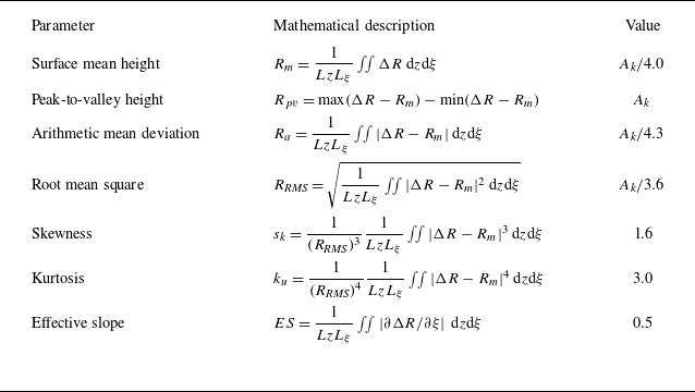
 Ak=λk/2
 Rcyl

 ρU
 Θ


 Θ=[5∘,15∘]
 cr≈0.5Ue

 99.5%h0,∞

 η=0.1

 Θ=[11.5∘,11.9∘]
 ρU

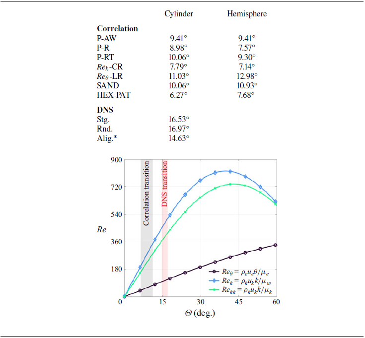
 Θtr


 f1=62
 f1=63
 f1=89

 η−z
 Θ


 η−z
 Θ=14∘
 Θ=12∘

 (f,β)=(69kHz,0)

 N
 f=75


 Q=5(1011)s−2
 z=0


 z=0


 N

 Open access

