1 Introduction
Over the last couple of decades, electrokinetic flow phenomena have received significant attention from the scientific community. Within the general framework of electrohydrodynamics (Castellanos Reference Castellanos and Castellanos1998), the motion of fluids carrying dissolved electric charges in an electric field as well as the transport of these charges relative to the carrier fluid is considered. Electrokinetics is of crucial importance in the stabilization and motion of particles in colloidal suspensions (Russel, Saville & Schowalter Reference Russel, Saville and Schowalter1989) and is relevant in electrospray-based fabrication methods (Salata Reference Salata2005) or DNA-manipulation/separation techniques (Viovy Reference Viovy2000), to name a few. Ion transport in dilute electrolytes is commonly captured by the Nernst–Planck equation. At moderate to high ion concentrations however, the finite size and the discrete nature of the ions have to be taken into account (Nadler et al. Reference Nadler, Schuss, Singer and Eisenberg2004). To capture the momentum transfer between ions and the solvent, the conventional stress tensor in the Navier–Stokes equation is supplemented by the Maxwell stresses. Being a manifestation of the Onsager reciprocal principle (Onsager Reference Onsager1931), the interaction between the dissolved ions and the liquid carrier goes along with two distinct types of electrokinetic coupling with single-phase fluids: one where an electric field drives a fluid motion such as in electroosmotic flow (EOF), and another where ions advected along with the fluid generate an electric field. While EOF and induced-charge EOF is well suited to propel fluid (Kim, Beskok & Kihm Reference Kim, Beskok and Kihm2002; Squires & Bazant Reference Squires and Bazant2004; Stone, Stroock & Ajdari Reference Stone, Stroock and Ajdari2004; Yossifon, Frankel & Miloh Reference Yossifon, Frankel and Miloh2006) or to enhance mixing in microchannels (Wang et al. Reference Wang, Chen, Lee, Yu and Chang2006; Barz, Zadeh & Ehrhard Reference Barz, Zadeh and Ehrhard2011), ion advection is described by the so-called streaming potential (SP) (Dukhin Reference Dukhin1993). It is relevant in a number of physical phenomena related to the advection of charged interfaces such as in the electroviscous drag enhancement observed in particle suspensions (Sherwood Reference Sherwood1980). In addition, it can be used to convert mechanical (and as will be shown also thermal) energy into electric energy (Yang et al. Reference Yang, Lu, Kostiuk and Kwok2003). This is, among others, in the focus of the current study.
Electrokinetic phenomena are commonly associated with the excess of one ion species in the vicinity of an interfacial charge of opposite polarity carried by submerged solid bodies or walls. The ions form a diffusion-dominated electric double layer (EDL) which screens the surface charge. Unlike the ions in the Stern layer, the ions in the EDL remain mobile and, as in electrokinetic streaming applications, can be advected with the flow. Depending on the bulk ion concentration, the EDL is typically only a few to a couple of hundred nm thick so that many studies of electrokinetic phenomena do not resolve the EDL, but assume an effective slip velocity (Smoluchowski limit). The liquid outside the EDL is irrelevant for the momentum source term driving the flow. By contrast, it contributes to the usually undesired ion flux by means of electromigration (i.e. the bulk conduction current) caused by the applied potential difference. Therefore, to minimize the detrimental influence of the bulk fluid, many studies on electrokinetics focus on system dimensions of the same order as the EDL thickness (the Debye parameter is of order unity) (van der Heyden, Stein & Dekker Reference van der Heyden, Stein and Dekker2005; Daguji Reference Daguji2009; Xie et al. Reference Xie, Sherwood, Shui, van den Berg and Eijkel2011). Most studies of the electrokinetic streaming potential are concerned with pressure-driven flow, while – in comparison – few investigations have been performed on shear-driven flow (Song & Wang Reference Song and Wang2004) or other sources of fluid propulsion. Owing to the superposition principle in Stokes flow, electrokinetic and pressure-driven flow fields can be linearly superimposed. As a result, the streaming potential becomes a linear function of the driving pressure difference.
To date, studies on thermal effects in electrokinetic flow are comparably scarce. Nevertheless, within the general scope of recent energy sustainability efforts, it is of interest to investigate thermally driven electrokinetic charge separation (Grosu & Bologa Reference Grosu and Bologa2010) based on using waste heat (generated, for example, by the central processing unit (CPU) of a computer). Most of the thermally induced fluid propulsion (by buoyancy, thermocapillarity or evaporation) can be formulated – at least in the Stokes limit – as an effective pressure difference or shear force, which can be subsequently combined with the conventional electrokinetic theory to estimate the streaming potential generated by a thermally propelled liquid. In this case, a combined study of thermal, fluid mechanical and electrokinetic effects does not appear to be necessary. This holds as long as other effects induced by a variation of temperature are negligible. Approximately four different non-isothermal contributions may enter the problem formulation: firstly, most of the bulk properties such as viscosity, diffusivities, electric conductivity and permittivity are temperature dependent. Under the application of direct (DC) (Wong & Melcher Reference Wong and Melcher1969) or alternating current (AC) (González et al.
Reference González, Ramos, Morgan, Green and Castellanos2006) voltages this may lead, for instance, to electrothermal convection. Secondly, dissipative effects occurring in the bulk, such as viscous dissipation and Joule heating (Zhao & Liao Reference Zhao and Liao2002; Maynes & Webb Reference Maynes and Webb2004; Sadeghi & Saidi Reference Sadeghi and Saidi2010), should be included in the energy equation as well. Thirdly, the formation of a wall (
 $\unicode[STIX]{x1D701}$
-) potential is strongly dependent on the dissociation processes of surface groups and ion absorption at the wall (Revil, Pezard & Glover Reference Revil, Pezard and Glover1999). More specifically, the wall potential is determined, at least under quasi-equilibrated conditions, by a temperature-dependent equilibrium constant, leading in turn to a temperature-dependent
 $\unicode[STIX]{x1D701}$
potential. This becomes particularly important for flow through porous media at elevated temperatures, as, for instance, treated in geophysical research studies (Ishido, Mizutani & Baba Reference Ishido, Mizutani and Baba1983; Reppert & Morgan Reference Reppert and Morgan2003). Lastly, similar to the thermal diffusion of colloidal particles in a non-isothermal liquid (Piazza Reference Piazza2004; Würger Reference Würger2010), the charge carriers in an electrolyte are also set into a thermally induced diffusive motion. Under the condition of local charge neutrality, steady state and the absence of any external pressure gradient, this leads to a well-known thermoelectric potential in bulk electrolytes (Guthrie, Wilson & Schomaker Reference Guthrie, Wilson and Schomaker1949). As briefly summarized in appendix A, this Seebeck-type of thermoelectric potential vanishes if the thermal mobilities of the ion species do not differ from each other. The effect is typically quantified in terms of a bulk Soret coefficient,
 $\unicode[STIX]{x1D70E}_{T}$
, and can be enhanced, for instance, by the utilization of more exotic electrolytes (Bonetti et al.
Reference Bonetti, Nakamae, Roger and Guenoun2011). In the context of such thermodiffusive processes, there has been a long standing interest in ion-selective membranes exposed to a temperature gradient (Hills, Jacobs & Lakshiminarayanaiah Reference Hills, Jacobs and Lakshiminarayanaiah1957; Gaeta et al.
Reference Gaeta, Ascolese, Bencivenga, Ortiz de Zárate, Pagliuca, Perna, Rossi and Mita1992), which are also relevant for the sensation of heat felt by humans (Tyrrell, Taylor & Williams Reference Tyrrell, Taylor and Williams1954). This interest was recently renewed in the realm of unconventional thermoelectric energy conversion (Sandbakk, Bentien & Kjelstrup Reference Sandbakk, Bentien and Kjelstrup2013). The classical description of membrane potentials is based on non-equilibrium thermodynamics and averaged transport numbers (Tasaka & Nagasawa Reference Tasaka and Nagasawa1978; Tasaka Reference Tasaka1986), without making specific reference to the ion distribution inside the pore. In fact, virtually all of these studies involving the Soret effect assume local charge neutrality. While this is valid in the bulk, the fluid within the EDL is not electroneutral. This is particularly relevant for electrokinetic flows through non-isothermal nanochannels, e.g. employed as an electrochemical thermal energy harvester (Kang et al.
Reference Kang, Fang, Kozlov, Haines, Li, Kim, Chen and Baughman2012). Numerical work on pressure-driven electrokinetic flow in a slit microchannel, which was ten times wider than the EDL and exhibited a
 $\unicode[STIX]{x1D701}$
potential of approximately
 $50\times 10^{-3}~\text{V}$
while the wall temperature increased along its length by approximately
 $17\,\%$
, indicates that in comparison to isothermal conditions, thermodiffusive and electrothermal effects may reduce or enhance the overall volumetric flow through the channel (Ghonge et al.
Reference Ghonge, Chakraborty, Dey and Chakraborty2013). Recent numerical simulations of a nanochannel of width twice the EDL thickness and with a
 $\unicode[STIX]{x1D701}$
potential of
 $50{-}100\times 10^{-3}~\text{V}$
suggest that viscous dissipation and Joule heating play a role only at higher salt concentrations for which however no EDL overlap, and thus no ion selectivity of the nanochannel, is present. It was shown that applying a temperature difference between both channel ends modifies the ion selectivity of the channel (Wood, Benneker & Lammertink Reference Wood, Benneker and Lammertink2016).
The present work focuses on the implications and significance of ion motion induced by a gradient in temperature in symmetric electrolytes in a confined geometry. Of special interest is the comparison between semi-analytical and full numerical models to identify the dominant non-isothermal effects within the different regimes of the characteristic parameters, especially of the EDL thickness scaled to the slit height (Debye parameter) and the wall
 $\unicode[STIX]{x1D701}$
potential. As a model system, a pressure-driven slit channel flow of a fully dissociated binary electrolyte, subject to a temperature gradient along the channel centre plane, is chosen. Unlike the classical treatments of thermoelectricity in bulk electrolytes, the condition of local charge neutrality is not enforced. In the course of the derivation, thermophoretic ion motion as well as the temperature dependencies of the electrophoretic ion mobility (equally referred to as ion electromobility) and the dielectric permittivity of the solvent are shown to be the dominant non-isothermal effects. A modified Boltzmann distribution is derived from the scaled, non-isothermal Nernst–Planck equation, taking advantage of the disparate ratio between channel height and channel length. This expression for the ion distribution leads to a correlation between the local EDL thickness and the local temperature. While a uniform growth of the EDL generally increases the streaming potential, the thermal gradient along the channel centre plane gives rise not only to a corresponding gradient in the EDL potential but, together with the temperature dependence of the ion electromobility and the space charge of the EDL, to a non-advective ion transport by means of selective (i.e. polarity-dependent) migration. In a recent work focusing on non-advective effects (Dietzel & Hardt Reference Dietzel and Hardt2016), the latter was shown to be dominant under extreme confinement, inducing for a vanishing Debye parameter a thermoelectric field of order
 $\unicode[STIX]{x1D701}/T$
, with
 $T$
being the absolute temperature. The current work explicitly includes advective effects and the gradient of the EDL potential along the channel (developing due to the combination of the relatively weak temperature-induced modification of the EDL thickness and the strong electric field within the EDL) leads to a gradient in electrohydrostatic (or, equivalently, in the electroosmotic) pressure and an additional axial Maxwell stress, whose superposition triggers an advective ion transport. While thermally induced osmotic pressure gradients are known to be responsible for the thermoosmotic propulsion of colloidal particles in a thermal gradient (Würger Reference Würger2010), as well as for the thermoosmotic transport across semi-permeable (but not explicitly charged) membranes (Dariel & Kedem Reference Dariel and Kedem1975), thermoosmotically induced electric fields have been attributed to the additional term arising in the Korteweg–Helmholtz force when the dielectric permittivity is not constant (Derjaguin, Churaev & Muller Reference Derjaguin, Churaev and Muller1987). The accurate description of the temperature-dependent EDL potential and its effect not only on the electroosmotic pressure but also on the Maxwell stress has not been achieved in any of these works. Considering that at isothermal conditions the electroosmotic ion pressure exactly cancels the Maxwell stress exerted by the EDL potential (so that the ion cloud of the EDL is in mechanical equilibrium), at non-uniform temperature the simultaneous consideration of the effect of temperature variations on the EDL potential, on the electroosmotic pressure and on the Maxwell stress is deemed imperative. Sasidhar & Ruckenstein (Reference Sasidhar and Ruckenstein1982) investigated a related scenario in the osmotic transport of an electrolyte through charged cylindrical pores, which are kept at uniform temperature but are subjected to an externally imposed axial concentration gradient. Nevertheless, so far and to the best of our knowledge, the thermoosmotically driven transport and the implications of such a flux on the electrokinetic streaming have never been explicitly and systematically addressed. This is the focus of the present study.
In § 2, an analytical model based on the Debye–Hückel (DH) approximation at low
 $\unicode[STIX]{x1D701}$
potential and a full numerical model of the local, non-isothermal streaming potential (in the form of a scaled, induced electric field) are developed. The latter is a function of the pressure and temperature difference, nominal Debye parameter,
 $\unicode[STIX]{x1D701}$
potential, Soret coefficient as well as of the temperature dependencies of dielectric permittivity and ion mobility. Counterintuitively, to leading order in the temperature difference, the temperature dependencies of viscosity, heat conductivity, heat capacity and Fickian diffusion coefficients have no effect. The thermally induced modifications of the EDL potential are discussed. In § 3, the induced streaming potential is analysed for specific limiting cases. Subsequently, in the limit of a vanishing external pressure difference, the thermoosmotically induced electric field is obtained by numerical integration along the channel centre plane for the case that both thermophoretic ion mobilities are the same and discussed for a realistic range of parameters. The full numerical model is compared to semi-analytical expressions valid within the DH approximation.
2 Model equations and perturbative solutions
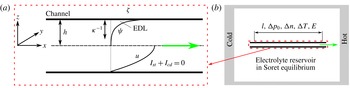
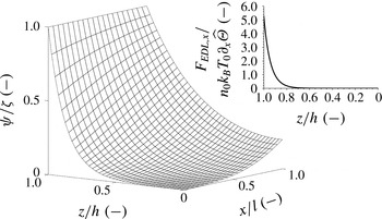
In the following, the governing equations are summarized and simplified to obtain analytical solutions for the flow field, along with its thermoosmotically driven contributions and the streaming potential inside a parallel-plate slit channel exposed to the combined action of an externally applied pressure (
 $\unicode[STIX]{x0394}p_{0}$
) and temperature difference (
 $\unicode[STIX]{x0394}T$
) between both ends of the channel, with the channel length denoted by
 $l$
and one half of its gap width denoted by
 $h$
, see figure 1(a). In such channels, the order of magnitude of the pressure-driven (isothermal) flow can be approximated by
 $u_{0}=\unicode[STIX]{x0394}p_{0}Ah/(3\unicode[STIX]{x1D702}_{0})$
(Poiseuille), where
 $A=h/l$
and
 $A^{2}\ll 1$
. The dynamic viscosity of the electrolyte
 $\unicode[STIX]{x1D702}_{0}$
is determined at the ambient reference temperature
 $T_{0}$
, where
 $\unicode[STIX]{x0394}T/T_{0}<1$
is assumed. The electrokinetic response of the channel is commonly a strong function of the non-dimensional Debye parameter
 $\overline{\unicode[STIX]{x1D705}}=\unicode[STIX]{x1D705}h$
, where
 $\unicode[STIX]{x1D705}^{-1}=\sqrt{\unicode[STIX]{x1D716}k_{B}T/(2e^{2}\unicode[STIX]{x1D708}^{2}n)}$
is the Debye length of the EDL near charged interfaces. The Boltzmann constant is denoted by
 $k_{B}$
,
 $e$
is the elementary charge,
 $\unicode[STIX]{x1D708}$
is the valence of the symmetric
 $\unicode[STIX]{x1D708}:\unicode[STIX]{x1D708}$
electrolyte and
 $n$
is the number concentration of the dissolved salt. Within the electroneutral regime, i.e. sufficiently far away from any charged wall, this equals the local ion number concentrations. With
 $\unicode[STIX]{x1D700}_{0}$
being the vacuum dielectric permittivity and
 $\unicode[STIX]{x1D700}_{r}$
being the relative permittivity of the liquid, its permittivity is given by
 $\unicode[STIX]{x1D716}=\unicode[STIX]{x1D700}_{0}\unicode[STIX]{x1D700}_{r}$
. Furthermore, the bulk electric conductivity of liquid electrolytes with dissolved salt ions as charge carriers of ionic mobility
 $\unicode[STIX]{x1D714}\approx D/(k_{B}T)$
can be approximated by
 $\unicode[STIX]{x1D70E}^{(\infty )}=2e^{2}\unicode[STIX]{x1D708}^{2}n\unicode[STIX]{x1D714}$
, where
 $D$
is a suitably averaged reference diffusion coefficient.
(a) Schematic drawing of a slit channel of length
 $l$
and half-gap width
 $h$
. The problem is assumed to be symmetric about the
 $x,y$
-plane and translationally invariant in the
 $y$
-direction. The flow profile
 $u$
, mainly driven by the axial pressure difference
 $\unicode[STIX]{x0394}p_{0}$
, is approximately parabolic with zero velocity at the shear plane, where the electric potential is equal to the
 $\unicode[STIX]{x1D701}$
potential. The latter is screened by ions in the EDL, leading to an internal potential distribution
 $\unicode[STIX]{x1D713}$
. No net charge is transported in the system, so that advective ion streaming generates a streaming current
 $I_{st}$
, which is exactly compensated by a conduction current
 $I_{cd}$
due to an induced (streaming) electric field
 $E$
. Apart from the pressure gradient, axial gradients in temperature,
 $\unicode[STIX]{x0394}T/l$
, and in salt concentration,
 $\unicode[STIX]{x0394}n/l$
are imposed. It is assumed that the salt concentrations at both ends of the channel,
 $\unicode[STIX]{x0394}n$
, are determined by thermodiffusion equivalent to the Soret equilibrium in bulk electrolytes. As illustrated in (b), this can be considered as if the channel were submerged in a large reservoir filled with the electrolyte at rest and subjected to the same temperature difference
 $\unicode[STIX]{x0394}T$
.

Herein, unlike conventional considerations of electrokinetic streaming in microchannels, the temperature is not constant and its distribution is governed by the energy equation. As also demonstrated in the supplemental material of Dietzel & Hardt (Reference Dietzel and Hardt2016), viscous dissipation and Joule heating are negligibly small (Wood et al.
Reference Wood, Benneker and Lammertink2016). Neglecting also the kinetic energy of the flow, the energy equation is given by
 $\unicode[STIX]{x1D70C}c_{p}d_{t}T=\unicode[STIX]{x1D735}\boldsymbol{\cdot }(k\unicode[STIX]{x1D735}T)$
, with
 $T$
being the absolute temperature. The substantial derivative
 $d_{t}\equiv \text{d}/\text{d}t$
is denoted by
 $d_{t}(\cdot )\equiv \unicode[STIX]{x2202}_{t}(\cdot )+\boldsymbol{v}\boldsymbol{\cdot }\unicode[STIX]{x1D735}(\cdot )$
with the velocity vector
 $\boldsymbol{v}=(u,w)$
. The slit geometry implies a vanishingly small velocity component in the
 $y$
-direction, so that this is readily omitted from the description. The fluid density, thermal conductivity and heat capacity at constant pressure are labelled by
 $\unicode[STIX]{x1D70C}$
,
 $k$
and
 $c_{p}$
, respectively. All thermophysical parameters of the solvent (
 $\unicode[STIX]{x1D702}$
,
 $\unicode[STIX]{x1D70C}$
,
 $c_{p}$
,
 $k$
,
 $\unicode[STIX]{x1D716}$
) as well as of the dissolved ions (
 $D$
,
 $\unicode[STIX]{x1D714}$
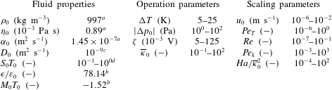
) are, in general, temperature dependent. Table 1 summarizes typical relative variations for aqueous solutions. To calculate the relative variations of
 $D$
and
 $\unicode[STIX]{x1D714}$
with temperature, the Stokes–Einstein relation
 $D\approx k_{B}T/(6\unicode[STIX]{x03C0}\unicode[STIX]{x1D702}R_{h})$
is used, where
 $R_{h}$
is the hydrodynamic radius of the ions. At least for
 $\text{Na}^{+}$
,
 $\text{K}^{+}$
and
 $\text{Cl}^{-}$
,
 $R_{h}$
is practically unaffected by temperature (the change is between
 $O(10^{-4})$
to low
 $O(10^{-3})~\text{K}^{-1}$
(Oelkers & Helgeson Reference Oelkers and Helgeson1989)). With this one finds
 $\unicode[STIX]{x2202}_{T}D/D=1/T-\unicode[STIX]{x2202}_{T}\unicode[STIX]{x1D702}/\unicode[STIX]{x1D702}$
and
 $\unicode[STIX]{x2202}_{T}\unicode[STIX]{x1D70E}^{(\infty )}/\unicode[STIX]{x1D70E}^{(\infty )}=\unicode[STIX]{x2202}_{T}\unicode[STIX]{x1D714}/\unicode[STIX]{x1D714}=-\unicode[STIX]{x2202}_{T}\unicode[STIX]{x1D702}/\unicode[STIX]{x1D702}$
. Given the very small concentration of dissociated water molecules in comparison to the salt ions, the electric conductivity of pure water,
 $\unicode[STIX]{x1D70E}^{(DI)}$
(stemming from the dissociated
 $\text{H}^{+}$
- and
 $\text{OH}^{-}$
-ions) is ignored. Therefore, we neglect the change of the electric conductivity of pure water with temperature. Hence, for the present purpose, the variations of the diffusivity and viscosity with temperature have the largest effects, while the change of the heat capacity and of the liquid density with temperature can be readily neglected. Furthermore, since liquids are virtually incompressible not only is
 $c_{p}\equiv c_{p,0}$
a constant but also
 $\unicode[STIX]{x1D70C}\equiv \unicode[STIX]{x1D70C}_{0}$
.
Relative variation of thermophysical properties with temperature in units of
 $10^{-3}~\text{K}^{-1}$
, determined at
 $25\,^{\circ }\text{C}$
(
 $T_{0}=298~\text{K}$
). The derivatives with respect to temperature of
 $\unicode[STIX]{x1D702}$
,
 $\unicode[STIX]{x1D70C}$
,
 $c_{p}$
,
 $k$
and
 $\unicode[STIX]{x1D716}$
were calculated by evaluating the respective parameter at
 $T_{0}+\unicode[STIX]{x0394}T$
minus the value at
 $T_{0}$
divided by
 $\unicode[STIX]{x0394}T=25~\text{K}$
(forward scheme). Tabulated data of Lide (Reference Lide and Lide2009) were used, except for
 $\unicode[STIX]{x1D70E}^{(DI)}$
, which was taken from Light & Licht (Reference Light and Licht1987). In addition,
 $\unicode[STIX]{x2202}_{T}D/D\approx 1/T-\unicode[STIX]{x2202}_{T}\unicode[STIX]{x1D702}/\unicode[STIX]{x1D702}$
and
 $\unicode[STIX]{x2202}_{T}\unicode[STIX]{x1D714}/\unicode[STIX]{x1D714}\approx -\unicode[STIX]{x2202}_{T}\unicode[STIX]{x1D702}/\unicode[STIX]{x1D702}$
.

The energy equation can be brought in a dimensionless form by scaling the axial
 $x$
-direction by
 $l$
while the lateral
 $z$
-coordinate is scaled by
 $h$
, i.e.
 $\boldsymbol{X}=(X,Z)=(x/l,z/h)$
. With
 $\unicode[STIX]{x1D6FC}_{0}=k_{0}/(c_{p,0}\unicode[STIX]{x1D70C}_{0})$
as the thermal (reference) diffusivity and
 $Pe_{T}=hu_{0}/\unicode[STIX]{x1D6FC}_{0}$
as the thermal Péclet number, one finds
 $$\begin{eqnarray}\displaystyle APe_{T}(d_{\unicode[STIX]{x1D70F}}\unicode[STIX]{x1D6E9})-A^{2}\left[\unicode[STIX]{x2202}_{X}\left(\frac{k}{k_{0}}\unicode[STIX]{x2202}_{X}\unicode[STIX]{x1D6E9}\right)\right]=\unicode[STIX]{x2202}_{Z}\left(\frac{k}{k_{0}}\unicode[STIX]{x2202}_{Z}\unicode[STIX]{x1D6E9}\right), & & \displaystyle\end{eqnarray}$$
where
 $\unicode[STIX]{x1D6E9}=(T-T_{0})/\unicode[STIX]{x0394}T$
is the non-dimensional temperature and
 $\unicode[STIX]{x2202}_{\unicode[STIX]{x1D711}}\equiv \unicode[STIX]{x2202}/\unicode[STIX]{x2202}\unicode[STIX]{x1D711}$
(
 $\unicode[STIX]{x1D711}=\unicode[STIX]{x1D70F},X,Z$
). In non-dimensional notation, the substantial derivative is denoted by
 $d_{\unicode[STIX]{x1D70F}}(\cdot )=\unicode[STIX]{x2202}_{\unicode[STIX]{x1D70F}}(\cdot )+\boldsymbol{V}\boldsymbol{\cdot }\overline{\unicode[STIX]{x1D735}}(\cdot )=(l/u_{0})d_{t}(\cdot )$
, with
 $\unicode[STIX]{x1D70F}=tu_{0}/l$
,
 $\overline{\unicode[STIX]{x1D735}}=(\unicode[STIX]{x2202}_{X},\unicode[STIX]{x2202}_{Z})$
and
 $\boldsymbol{V}=(U,W)=(u/u_{0},w/w_{0})$
. As implied by the non-dimensional continuity equation,
 $\overline{\unicode[STIX]{x1D735}}\boldsymbol{\cdot }\boldsymbol{V}$
, the vertical scaling velocity is
 $w_{0}=Au_{0}$
. It is assumed that
 $h$
is much smaller than the axial extent
 $l$
and thus
 $A^{2}\ll 1$
. As will be shown later using table 3 in § 3.3, for simple electrolytes in typical applications of pressure-driven streaming in microchannels
 $Pe_{T}\lesssim O(A)$
. Hence, the left-hand side of (2.1) can be neglected up to first order in
 $A$
. Using the symmetry condition along the centre plane at
 $Z=0$
, it follows that the temperature is identical to the local wall temperature. It is assumed here that a linear temperature profile along
 $X$
is imposed on the channel wall, so that also the liquid temperature varies according to
 $\unicode[STIX]{x2202}_{X}\unicode[STIX]{x1D6E9}=\text{const.}$
, while
 $\unicode[STIX]{x2202}_{Z}\unicode[STIX]{x1D6E9}=0$
. Hence, in the present limit, the temperature dependence of the thermal conductivity of the liquid is of no importance.
2.1 General axial velocity profile
The motion of an incompressible electrolyte of density
 $\unicode[STIX]{x1D70C}\equiv \unicode[STIX]{x1D70C}_{0}$
and mass-averaged velocity vector
 $\boldsymbol{v}$
is described by the Navier–Stokes equation
 $\unicode[STIX]{x1D70C}d_{t}\boldsymbol{v}=\unicode[STIX]{x1D735}\boldsymbol{\cdot }\unicode[STIX]{x1D748}^{V}+\unicode[STIX]{x1D735}\boldsymbol{\cdot }\unicode[STIX]{x1D748}^{M}$
with Maxwell stresses added as a source term. The mechanical stress tensor is denoted by
 $\unicode[STIX]{x1D748}^{V}=-p\unicode[STIX]{x1D644}+\unicode[STIX]{x1D702}[\unicode[STIX]{x1D735}\boldsymbol{v}+(\unicode[STIX]{x1D735}\boldsymbol{v})^{\text{T}}]$
with
 $\unicode[STIX]{x1D644}$
being the unit tensor,
 $p$
the liquid pressure and where the dynamic viscosity
 $\unicode[STIX]{x1D702}$
does not necessarily need to be constant but might vary with temperature. The assumed small channel size allows us to omit hydrostatic contributions, and the channel is aligned orthogonal to the direction of the gravitational acceleration
 $\boldsymbol{g}$
to remove buoyancy effects (
 $\unicode[STIX]{x1D735}T\boldsymbol{\cdot }\boldsymbol{g}=0$
). For a homogeneous, incompressible fluid, the Maxwell stress tensor reads
 $\unicode[STIX]{x1D748}^{M}=\unicode[STIX]{x1D716}(\unicode[STIX]{x1D735}\unicode[STIX]{x1D719}\unicode[STIX]{x1D735}\unicode[STIX]{x1D719}-\unicode[STIX]{x1D735}\unicode[STIX]{x1D719}\boldsymbol{\cdot }\unicode[STIX]{x1D735}\unicode[STIX]{x1D719}\unicode[STIX]{x1D644}/2)$
, where
 $\unicode[STIX]{x1D719}$
is the electric potential. The force contribution due to the Maxwell stress tensor can be expressed in terms of the Korteweg–Helmholtz electric force per volume given by
 $\unicode[STIX]{x1D735}\boldsymbol{\cdot }\unicode[STIX]{x1D748}^{M}=-\unicode[STIX]{x1D70C}_{f}\unicode[STIX]{x1D735}\unicode[STIX]{x1D719}-(\unicode[STIX]{x1D735}\unicode[STIX]{x1D719})^{2}\unicode[STIX]{x1D716}_{T}\unicode[STIX]{x1D735}T/2$
(Russel et al.
Reference Russel, Saville and Schowalter1989), where the temperature dependence of the dielectric permittivity was incorporated by
 $\unicode[STIX]{x1D735}\unicode[STIX]{x1D716}=\unicode[STIX]{x1D716}_{T}\unicode[STIX]{x1D735}T$
, with
 $\unicode[STIX]{x1D716}_{T}\equiv \text{d}\unicode[STIX]{x1D716}/\text{d}T$
. The charge density
 $\unicode[STIX]{x1D70C}_{f}$
is related to
 $\unicode[STIX]{x1D719}$
according to the Poisson equation
 $\unicode[STIX]{x1D735}\boldsymbol{\cdot }(\unicode[STIX]{x1D716}\unicode[STIX]{x1D735}\unicode[STIX]{x1D719})=-\unicode[STIX]{x1D70C}_{f}$
. The common assumption of electrokinetics is made that
 $\unicode[STIX]{x1D719}=\unicode[STIX]{x1D713}+\unicode[STIX]{x1D719}_{0}$
is a linear superposition of the electric potential due to the ion double layer at the interfaces,
 $\unicode[STIX]{x1D713}(x,z)$
, measuring the departure from electroneutrality (Fair & Osterle Reference Fair and Osterle1971), while
 $\unicode[STIX]{x1D719}_{0}$
is an induced electric potential with vanishing affiliated charge density (source free). Hence, the Laplace operator acting on
 $\unicode[STIX]{x1D719}_{0}$
vanishes. Along with the symmetry condition at the channel centre plane, this implies that
 $\unicode[STIX]{x1D719}_{0}=\unicode[STIX]{x1D719}_{0}(x)$
and
 $d_{x}\unicode[STIX]{x1D719}_{0}\equiv -E$
is a constant. As will be further discussed in § 2.2,
 $E$
is calculated by integrating the axial velocity profile over the channel cross-section. In non-dimensional form, the Poisson equation reads
 $$\begin{eqnarray}\displaystyle A^{2}(\unicode[STIX]{x2202}_{X}^{2}\unicode[STIX]{x1D6F7}+M\unicode[STIX]{x0394}T\unicode[STIX]{x2202}_{X}\unicode[STIX]{x1D6F7}\unicode[STIX]{x2202}_{X}\unicode[STIX]{x1D6E9})+\unicode[STIX]{x2202}_{Z}^{2}\unicode[STIX]{x1D6F9}+M\unicode[STIX]{x0394}T\unicode[STIX]{x2202}_{Z}\unicode[STIX]{x1D6F9}\unicode[STIX]{x2202}_{Z}\unicode[STIX]{x1D6E9}=-\frac{1}{2}\overline{\unicode[STIX]{x1D705}}_{M}^{2}\frac{\unicode[STIX]{x1D70C}_{f}}{e\unicode[STIX]{x1D708}n_{0}}, & & \displaystyle\end{eqnarray}$$
where
 $M=\unicode[STIX]{x1D716}_{T}/\unicode[STIX]{x1D716}$
, while
 $(\unicode[STIX]{x1D6F7},\unicode[STIX]{x1D6F9})=(\unicode[STIX]{x1D719},\unicode[STIX]{x1D713})e\unicode[STIX]{x1D708}/(k_{B}T_{0})$
and
 $\overline{\unicode[STIX]{x1D705}}_{M}$
are the dimensionless potentials and the Debye parameter, respectively. In (2.2), it was already taken into account that
 $E$
is a constant so that
 $\unicode[STIX]{x2202}_{Z}\unicode[STIX]{x1D6F7}\equiv \unicode[STIX]{x2202}_{Z}\unicode[STIX]{x1D6F9}$
(and thus,
 $\unicode[STIX]{x2202}_{Z}^{2}\unicode[STIX]{x1D6F7}\equiv \unicode[STIX]{x2202}_{Z}^{2}\unicode[STIX]{x1D6F9}$
as well). Expression (2.2) implies that, to leading order in
 $A$
, the charge density only affects the electric field components in the
 $Z$
-direction. Since the electric potentials are non-dimensionalized by
 $e\unicode[STIX]{x1D708}/(k_{B}T_{0})$
, the reference temperature in
 $\overline{\unicode[STIX]{x1D705}}_{M}$
equals
 $T_{0}$
. Nevertheless,
 $\overline{\unicode[STIX]{x1D705}}_{M}$
is not a constant but depends on the local value of
 $\unicode[STIX]{x1D716}$
and can be expressed by
 $$\begin{eqnarray}\displaystyle \overline{\unicode[STIX]{x1D705}}_{M} & = & \displaystyle \overline{\unicode[STIX]{x1D705}}_{0}\sqrt{\frac{\unicode[STIX]{x1D716}_{0}}{\unicode[STIX]{x1D716}}}=\overline{\unicode[STIX]{x1D705}}_{0}(1+M_{0}\unicode[STIX]{x0394}T\unicode[STIX]{x1D6E9})^{-1/2}\nonumber\\ \displaystyle & {\approx} & \displaystyle \overline{\unicode[STIX]{x1D705}}_{0}\left(1-\frac{1}{2}M_{0}\unicode[STIX]{x0394}T\unicode[STIX]{x1D6E9}\right),\end{eqnarray}$$
where
 $\overline{\unicode[STIX]{x1D705}}_{0}=\unicode[STIX]{x1D705}_{0}h$
,
 $M_{0}=\unicode[STIX]{x1D716}_{T}/\unicode[STIX]{x1D716}_{0}$
, and
 $\unicode[STIX]{x1D705}_{0}^{-1}=\sqrt{\unicode[STIX]{x1D716}_{0}k_{B}T_{0}/(2e^{2}\unicode[STIX]{x1D708}^{2}n_{0})}$
denotes the nominal EDL thickness for which all parameters are evaluated at the reference temperature
 $T_{0}$
so that
 $\unicode[STIX]{x1D716}=\unicode[STIX]{x1D716}_{0}$
and
 $n=n_{0}$
. Furthermore, the velocity field is obtained from the Navier–Stokes equation. The non-dimensional axial velocity component fulfils
 $$\begin{eqnarray}\displaystyle & & \displaystyle ARe(d_{\unicode[STIX]{x1D70F}}U)-A^{2}(\overline{\unicode[STIX]{x1D702}}\unicode[STIX]{x2202}_{X}^{2}U+2\unicode[STIX]{x2202}_{X}U\unicode[STIX]{x2202}_{X}\overline{\unicode[STIX]{x1D702}}+\unicode[STIX]{x2202}_{X}W\unicode[STIX]{x2202}_{Z}\overline{\unicode[STIX]{x1D702}})\nonumber\\ \displaystyle & & \displaystyle \quad -\,A^{2}\frac{Ha}{\overline{\unicode[STIX]{x1D705}}_{M}^{2}}\left\{\unicode[STIX]{x2202}_{X}^{2}\unicode[STIX]{x1D6F7}\unicode[STIX]{x2202}_{X}\unicode[STIX]{x1D6F7}+M\unicode[STIX]{x0394}T\left[\unicode[STIX]{x2202}_{X}\unicode[STIX]{x1D6F7}\unicode[STIX]{x2202}_{X}\unicode[STIX]{x1D6F7}-\frac{1}{2}(\unicode[STIX]{x2202}_{X}\unicode[STIX]{x1D6F7})^{2}\right]\unicode[STIX]{x2202}_{X}\unicode[STIX]{x1D6E9}\right\}=-\unicode[STIX]{x2202}_{X}P\nonumber\\ \displaystyle & & \displaystyle \quad +\,\unicode[STIX]{x2202}_{Z}(\overline{\unicode[STIX]{x1D702}}\unicode[STIX]{x2202}_{Z}U)+\frac{Ha}{\overline{\unicode[STIX]{x1D705}}_{M}^{2}}\left\{\unicode[STIX]{x2202}_{Z}^{2}\unicode[STIX]{x1D6F9}\unicode[STIX]{x2202}_{X}\unicode[STIX]{x1D6F7}+M\unicode[STIX]{x0394}T\left[\unicode[STIX]{x2202}_{Z}\unicode[STIX]{x1D6F9}\unicode[STIX]{x2202}_{X}\unicode[STIX]{x1D6F7}\unicode[STIX]{x2202}_{Z}\unicode[STIX]{x1D6E9}-\frac{1}{2}(\unicode[STIX]{x2202}_{Z}\unicode[STIX]{x1D6F7})^{2}\unicode[STIX]{x2202}_{X}\unicode[STIX]{x1D6E9}\right]\right\},\hspace{12.0pt}\end{eqnarray}$$
while the lateral component is obtained from
 $$\begin{eqnarray}\displaystyle & & \displaystyle A^{3}Re(d_{\unicode[STIX]{x1D70F}}W)-A^{2}(A^{2}\overline{\unicode[STIX]{x1D702}}\unicode[STIX]{x2202}_{X}^{2}W+\overline{\unicode[STIX]{x1D702}}\unicode[STIX]{x2202}_{Z}^{2}W+A^{2}\unicode[STIX]{x2202}_{X}W\unicode[STIX]{x2202}_{X}\overline{\unicode[STIX]{x1D702}}+2\unicode[STIX]{x2202}_{Z}W\unicode[STIX]{x2202}_{Z}\overline{\unicode[STIX]{x1D702}}+\unicode[STIX]{x2202}_{Z}U\unicode[STIX]{x2202}_{X}\overline{\unicode[STIX]{x1D702}})\nonumber\\ \displaystyle & & \displaystyle \quad -\,A^{2}\frac{Ha}{\overline{\unicode[STIX]{x1D705}}_{M}^{2}}\left\{\unicode[STIX]{x2202}_{X}^{2}\unicode[STIX]{x1D6F7}\unicode[STIX]{x2202}_{Z}\unicode[STIX]{x1D6F7}+M\unicode[STIX]{x0394}T\left[\unicode[STIX]{x2202}_{X}\unicode[STIX]{x1D6F7}\unicode[STIX]{x2202}_{Z}\unicode[STIX]{x1D6F7}\unicode[STIX]{x2202}_{X}\unicode[STIX]{x1D6E9}-\frac{1}{2}(\unicode[STIX]{x2202}_{X}\unicode[STIX]{x1D6F7})^{2}\unicode[STIX]{x2202}_{Z}\unicode[STIX]{x1D6E9}\right]\right\}=-\unicode[STIX]{x2202}_{Z}P\nonumber\\ \displaystyle & & \displaystyle \quad +\,\frac{Ha}{\overline{\unicode[STIX]{x1D705}}_{M}^{2}}\left\{\unicode[STIX]{x2202}_{Z}^{2}\unicode[STIX]{x1D6F9}\unicode[STIX]{x2202}_{Z}\unicode[STIX]{x1D6F7}+M\unicode[STIX]{x0394}T\left[\unicode[STIX]{x2202}_{Z}\unicode[STIX]{x1D6F9}\unicode[STIX]{x2202}_{Z}\unicode[STIX]{x1D6F7}-\frac{1}{2}(\unicode[STIX]{x2202}_{Z}\unicode[STIX]{x1D6F7})^{2}\right]\unicode[STIX]{x2202}_{Z}\unicode[STIX]{x1D6E9}\right\}.\end{eqnarray}$$
In this formulation, the charge density
 $\unicode[STIX]{x1D70C}_{f}$
was expressed by (2.2),
 $Re=\unicode[STIX]{x1D70C}u_{0}h/\unicode[STIX]{x1D702}_{0}$
is the Reynolds number and
 $\overline{\unicode[STIX]{x1D702}}=\unicode[STIX]{x1D702}/\unicode[STIX]{x1D702}_{0}$
is the non-dimensional local viscosity. Further,
 $Ha=2Ahn_{0}k_{B}T_{0}/(u_{0}\unicode[STIX]{x1D702}_{0})$
is the (scaled) Hartmann number, which compares the velocity induced by the osmotic reference pressure,
 $n_{0}k_{B}T_{0}$
, to the characteristic velocity scale. The fluid pressure is non-dimensionalized according to
 $P=Ahp/(u_{0}\unicode[STIX]{x1D702}_{0})$
. In Poiseuille-type flow with constant
 $\unicode[STIX]{x0394}p$
, the characteristic velocity
 $u_{0}$
is proportional to
 $A$
(see expression at the beginning of § 2). For sufficiently viscous fluids and sufficiently small values of
 $\unicode[STIX]{x0394}p$
and
 $h$
, one obtains
 $u_{0}\leqslant O(A)$
. Hence, with
 $A<1$
,
 $u_{0}$
can be expected to be a sufficiently small quantity, suggesting that the
 $Re$
number is small at least to order
 $A$
as well. In addition it follows that
 $Ha$
and
 $P$
do not depend on
 $A$
. For low
 $Re$
number flows in small-scale geometries, diffusion processes typically dominate over advective transport so that the ionic Péclet number
 $Pe_{k}=lu_{0}/D_{k}$
of ion species
 $k=(+,-)$
can be assumed to be not larger than
 $O(1)$
. As discussed by Yariv, Schnitzer & Frankel (Reference Yariv, Schnitzer and Frankel2011),
 $Ha$
cannot be of the same order as
 $Pe_{k}$
. In fact, also with the present scaling one has
 $Ha=(\unicode[STIX]{x1D70D}/Pe_{k})\overline{\unicode[STIX]{x1D705}}_{M}^{2}$
, where
 $\unicode[STIX]{x1D70D}=\unicode[STIX]{x1D716}/(\unicode[STIX]{x1D702}_{0}D)[k_{B}T_{0}/(\unicode[STIX]{x1D708}e)]^{2}$
is the intrinsic Péclet number (Saville Reference Saville1977). For typical aqueous solutions
 $\unicode[STIX]{x1D70D}\approx 0.5$
. Consequently,
 $Ha/\overline{\unicode[STIX]{x1D705}}_{M}^{2}\approx Ha/\overline{\unicode[STIX]{x1D705}}_{0}^{2}\leqslant O(1)$
is a consistent, and for the present purpose sufficient, scaling. As will be detailed in § 3, table 3 summarizes the validity of the assumptions made. While
 $\unicode[STIX]{x2202}_{Z}\unicode[STIX]{x1D6F7}\equiv \unicode[STIX]{x2202}_{Z}\unicode[STIX]{x1D6F9}$
, it was shown earlier that herein
 $\unicode[STIX]{x2202}_{Z}\unicode[STIX]{x1D6E9}=0$
. Neglecting terms of order
 $A^{2}$
and higher, one can deduce from (2.5) that
 $P\approx Ha/(2\overline{\unicode[STIX]{x1D705}}_{M}^{2})(\unicode[STIX]{x2202}_{Z}\unicode[STIX]{x1D6F9})^{2}+c_{1}(X)$
where
 $c_{1}(X)$
is an integration constant, which simply equals the externally applied pressure
 $P_{0}(X)$
. The first term proportional to the square of the lateral electric field is the electrostatic pressure contribution, representing the electroosmotic pressure of the ion cloud,
 $p_{osm}=nk_{B}T$
. In common studies of electrokinetic streaming in long (micro) channels, this term is not a function of the axial coordinate
 $X$
. By contrast, as will be shown later, the thickness of the EDL and the EDL potential are herein a function of temperature. Therefore, the electrostatic pressure varies in the axial direction, and the overall axial pressure gradient reads
 $\unicode[STIX]{x2202}_{X}P=Ha/(2\overline{\unicode[STIX]{x1D705}}_{M}^{2})[\unicode[STIX]{x2202}_{X}(\unicode[STIX]{x2202}_{Z}\unicode[STIX]{x1D6F9})^{2}-2(\unicode[STIX]{x2202}_{Z}\unicode[STIX]{x1D6F9})^{2}\unicode[STIX]{x2202}_{X}\overline{\unicode[STIX]{x1D705}}_{M}/\overline{\unicode[STIX]{x1D705}}_{M}]+\unicode[STIX]{x2202}_{X}P_{0}$
. With
 $Re=O(A)$
and
 $Ha/\overline{\unicode[STIX]{x1D705}}_{M}^{2}\leqslant O(1)$
, the left-hand side of (2.4) is small to order
 $A^{2}$
and one can write
 $$\begin{eqnarray}\displaystyle \unicode[STIX]{x2202}_{Z}(\overline{\unicode[STIX]{x1D702}}\unicode[STIX]{x2202}_{Z}U)\approx \frac{Ha}{\overline{\unicode[STIX]{x1D705}}_{M}^{2}}[\unicode[STIX]{x2202}_{X}(\unicode[STIX]{x2202}_{Z}\unicode[STIX]{x1D6F9})^{2}-\unicode[STIX]{x2202}_{Z}(\unicode[STIX]{x2202}_{Z}\unicode[STIX]{x1D6F9}\unicode[STIX]{x2202}_{X}\unicode[STIX]{x1D6F7})+(\unicode[STIX]{x2202}_{Z}\unicode[STIX]{x1D6F9})^{2}M\unicode[STIX]{x0394}T\unicode[STIX]{x2202}_{X}\unicode[STIX]{x1D6E9}]+\unicode[STIX]{x2202}_{X}P_{0}. & & \displaystyle\end{eqnarray}$$
In general, the viscosity is a function of the shear rate, concentration of dissolved species as well as of temperature. Shear rates are assumed to be sufficiently small so that shear thinning or thickening behaviour is of no importance, i.e. a Newtonian fluid behaviour is assumed. Furthermore, significant relative concentration changes of the dissolved ions are only present in the EDL. Absolute values of ion concentration are proportional to
 $n_{0}$
which is typically very small in dilute electrolytes. Therefore, even within the EDL, the dependence of the viscosity on the local ion concentration is expected to be negligibly small. Finally, the temperature varies only in the axial direction and (2.6) can be integrated twice in
 $Z$
even without explicit knowledge of the viscosity–temperature relationship. Symmetry is assumed at
 $Z=0$
(subscript
 $c$
), while the no-slip condition has to be fulfilled at the wall (
 $Z=1$
, subscript
 $s$
). With
 $\unicode[STIX]{x2202}_{X}\unicode[STIX]{x1D6F7}=\unicode[STIX]{x2202}_{X}\unicode[STIX]{x1D6F9}-\overline{E}$
, this leads to the expression for the axial velocity
 $$\begin{eqnarray}\displaystyle U=-\frac{\unicode[STIX]{x2202}_{X}P_{0}}{2\overline{\unicode[STIX]{x1D702}}}(1-Z^{2})+\frac{Ha}{\overline{\unicode[STIX]{x1D702}}\hspace{1.7pt}\overline{\unicode[STIX]{x1D705}}_{M}^{2}}\overline{E}(\unicode[STIX]{x1D6F9}-\overline{\unicode[STIX]{x1D701}})+\frac{Ha}{\overline{\unicode[STIX]{x1D702}}\hspace{1.7pt}\overline{\unicode[STIX]{x1D705}}_{M}^{2}}[\unicode[STIX]{x1D6FA}-\unicode[STIX]{x1D6FA}_{s}+\unicode[STIX]{x2202}_{Z}\unicode[STIX]{x1D6FA}_{c}(1-Z)], & & \displaystyle\end{eqnarray}$$
where
 $\overline{E}=e\unicode[STIX]{x1D708}lE/(k_{B}T_{0})$
. Note that the local dimensionless viscosity still depends on the axial coordinate, i.e.
 $\overline{\unicode[STIX]{x1D702}}=f(X)$
. In expression (2.7), the
 $\unicode[STIX]{x1D701}$
potential has been made dimensionless by
 $\overline{\unicode[STIX]{x1D701}}=\unicode[STIX]{x1D701}e\unicode[STIX]{x1D708}/(k_{B}T_{0})$
. Subsequently, at the present level of approximation, the
 $\unicode[STIX]{x1D701}$
potential will be assumed to be unaffected by temperature. This important issue and the suitability of that assumption will be discussed in more detail in the last paragraph of § 2.2.2. Furthermore, one has
 $$\begin{eqnarray}\displaystyle \unicode[STIX]{x1D6FA}=\iint \unicode[STIX]{x2202}_{X}(\unicode[STIX]{x2202}_{Z}\unicode[STIX]{x1D6F9})^{2}\,\text{d}^{2}Z-\int \unicode[STIX]{x2202}_{Z}\unicode[STIX]{x1D6F9}\unicode[STIX]{x2202}_{X}\unicode[STIX]{x1D6F9}\,\text{d}Z+\unicode[STIX]{x2202}_{X}\unicode[STIX]{x1D6E9}M\unicode[STIX]{x0394}T\iint (\unicode[STIX]{x2202}_{Z}\unicode[STIX]{x1D6F9})^{2}\,\text{d}^{2}Z, & & \displaystyle\end{eqnarray}$$
where the integration symbols denote primitives of the corresponding functions and
 $\text{d}^{2}Z$
denotes double integration of the integrand with respect to
 $Z$
. In (2.8), the first two integrals are the sum of the electrohydrostatic (EHS) contribution and the electromigration force (EMF), while the EHS alone is just one half of the first integral. For reasons of symmetry, one has
 $\unicode[STIX]{x2202}_{Z}\unicode[STIX]{x1D6F9}_{c}=0$
and thus also
 $\unicode[STIX]{x2202}_{Z}\unicode[STIX]{x1D6FA}_{c}=0$
. The expression for
 $\unicode[STIX]{x1D6FA}$
vanishes if the EDL potential
 $\unicode[STIX]{x1D6F9}$
does not depend on the axial coordinate and the temperature dependence of the permittivity is neglected. In this case, equation (2.7) resembles the well-known isothermal result. For further evaluation, a closing relation between the axial velocity
 $U$
, the electric potential
 $\unicode[STIX]{x1D6F9}$
and the induced electric field
 $\overline{E}$
is required.
2.2 Double-layer potential
2.2.1 Ion distribution
Despite known mathematical inconsistencies (Dreyer, Guhlke & Müller Reference Dreyer, Guhlke and Müller2013), for ion concentrations below
 $1~\text{M}$
(
 $\text{M}\equiv \text{mol}~\text{dm}^{-3}$
) (Levine, Marriott & Robinson Reference Levine, Marriott and Robinson1975) and sufficiently small temperature gradients and electric fields, the transport of
 $k=1,\ldots ,K$
ion species in liquids is commonly described by the Nernst–Planck equations reading
 $$\begin{eqnarray}\displaystyle d_{t}n_{k}=\unicode[STIX]{x1D735}\boldsymbol{\cdot }(D_{k}\unicode[STIX]{x1D735}n_{k}+n_{k}D_{T,k}\unicode[STIX]{x1D735}T+e\unicode[STIX]{x1D708}_{k}n_{k}\unicode[STIX]{x1D714}_{k}\unicode[STIX]{x1D735}\unicode[STIX]{x1D719}). & & \displaystyle\end{eqnarray}$$
The number concentration of positive or negative ions labelled with
 $k=(+,-)$
is referred to by
 $n_{k}$
. The diffusion coefficients affiliated with concentration gradients are
 $D_{k}$
, while
 $D_{T,k}$
are the thermophoretic mobility (i.e. thermodiffusion) coefficients of the ions when subjected to a temperature difference. The ionic mobilities under the action of a gradient in the electric potential,
 $\unicode[STIX]{x1D735}\unicode[STIX]{x1D719}$
, are given by
 $\unicode[STIX]{x1D714}_{k}\approx D_{k}/(k_{B}T)$
.
Thermal diffusion in multi-component fluids is frequently described in terms of so-called heats of transport,
 $Q_{k}$
(Helfand Reference Helfand1960), or, equivalently, entropies of transport
 $s_{k}=Q_{k}/T$
(Tasaka Reference Tasaka1986). As summarized in appendix A, these quantities are accurately defined within the phenomenological theory of non-equilibrium thermodynamics (Fitts Reference Fitts1962; de Groot & Mazur Reference de Groot and Mazur1984) and emerge from a cross-correlation between heat transport due to material fluxes on the one hand and matter transport due to thermal gradients on the other. Related phenomena are commonly termed heat–matter cross-effects. Equivalently, a concentration gradient of one species may lead, apart from the regular Fickian diffusion of that species, to diffusion of another, which is commonly termed cross-diffusion. The problem under study comprises a tertiary mixture of electrically neutral solvent with two ion species. In such a setting, cross-diffusion can be omitted if electroneutrality is assumed throughout the fluid domain, simplifying the problem to that of an effective binary mixture involving only a single linearly independent concentration field and a single non-advective ion flux (Haase Reference Haase1969). By contrast, as particularly relevant for nanochannel flow, electrolytes close to walls carrying a surface charge are not electrically neutral. The problem remains tertiary with linearly independent species concentrations, so that, according to the theoretical framework referred to, in principle cross-diffusional effects need to be considered explicitly. This is routinely neglected in most studies of electrokinetic streaming involving wall effects, in which ion transport is described by the (isothermal) Nernst–Planck equation. Adding thermophoretic ion diffusion to this equation in terms of
 $Q_{k}$
might give the misleading impression that the resulting equation is fully consistent with non-equilibrium thermodynamics (needed to define the
 $Q_{k}$
), although this would only be the case if cross-diffusional fluxes between different ion species were included (see for instance (A 11) of appendix A). To avoid this source of confusion and to emphasize the (still) limited validity of (2.9), instead of
 $Q_{k}$
, effective thermal diffusion coefficients
 $D_{T,k}$
are used herein. Nevertheless, within the present approximation, the distinction between
 $D_{T,k}$
and
 $Q_{k}$
has solely a cosmetic character. In fact, in appendix A it is shown that (herein)
 $S_{k}\equiv Q_{k}/(k_{B}T^{2})$
(Würger Reference Würger2010), where
 $S_{k}=D_{T,k}/D_{k}$
are the intrinsic Soret coefficients, (other authors would call it the thermal diffusion ratio) of the ions in units of
 $\text{K}^{-1}$
(Vigolo, Buzzaccaro & Piazza Reference Vigolo, Buzzaccaro and Piazza2010). In this context, it is important to point out that all of these parameters equivalently quantifying the thermomobility of individual ion species (
 $Q_{k}$
,
 $D_{T,k}$
or
 $S_{k}$
) can be determined experimentally only relative to each other (Hills et al.
Reference Hills, Jacobs and Lakshiminarayanaiah1957) and not on an absolute scale. Typically, as a point of reference, the thermophoretic mobility of the
 $\text{Cl}^{-}$
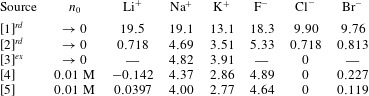
-ion is arbitrarily set to zero. Table 2 summarizes values of intrinsic Soret coefficients of common monovalent ions as derived from data found in the literature. Experimental data are usually reported in terms of ionic heats of transport
 $Q_{m,0,k}$
, in units of
 $\text{J}(\text{mol})^{-1}$
and for
 $T=T_{0}=298~\text{K}$
. To arrive at
 $S_{0,k}$
in units of
 $\text{K}^{-1}$
, the following conversion was used
 $$\begin{eqnarray}\displaystyle S_{0,k}=\frac{Q_{m,0,k}}{N_{A}k_{B}T_{0}^{2}}, & & \displaystyle\end{eqnarray}$$
where
 $N_{A}$
is the Avogadro constant. The experiments to determine
 $Q_{m,0,k}$
were conducted at a salt concentration of
 $n_{0}=0.01~\text{M}$
. Given that a full theoretical treatment is achievable only in the limit of infinite dilution, in some cases the experimental values were extrapolated towards
 $n_{0}\rightarrow 0$
, either using graphical extrapolation (Snowdon & Turner Reference Snowdon and Turner1960a
) or a reduction rule (Takeyama & Nakashima Reference Takeyama and Nakashima1988). As apparent from table 2,
 $S_{0,k}$
are generally
 $O(10^{-3})$
–
 $O(10^{-2})~\text{K}^{-1}$
. Values taken from Takeyama & Nakashima (Reference Takeyama and Nakashima1983) and listed in the first row are an order of magnitude larger than corresponding values reported by other authors. Considering entries listed in rows 2–5 only, the
 $S_{0,k}$
of one ion species in cation/anion combinations of
 $\text{Na}^{+}$
or
 $\text{K}^{+}$
with
 $\text{F}^{-}$
as well as
 $\text{Li}^{+}$
with
 $\text{Cl}^{-}$
or
 $\text{Br}^{-}$
is similar to that of the respective counter ion. By contrast, the corresponding values of each ion species in combinations of
 $\text{Na}^{+}$
or
 $\text{K}^{+}$
with
 $\text{Cl}^{-}$
or
 $\text{Br}^{-}$
as well as
 $\text{Li}^{+}$
with
 $\text{F}^{-}$
differ substantially.
Literature values for the intrinsic Soret coefficients
 $S_{0,k}$
in units of
 $10^{-3}~\text{K}^{-1}$
. All values were determined at
 $T_{0}=298~\text{K}$
. Experiments were conducted at a concentration of
 $n_{0}=0.01~\text{M}$
. Values reported at infinite dilution (
 $n_{0}\rightarrow 0$
) are determined from experimental values obtained at finite concentration either by graphical extrapolation (‘ex’) or using a reduction rule (‘rd’). [1] – Takeyama & Nakashima (Reference Takeyama and Nakashima1983), [2] – Takeyama & Nakashima (Reference Takeyama and Nakashima1988), [3] – Snowdon & Turner (Reference Snowdon and Turner1960a
), [4] – Agar & Turner (Reference Agar and Turner1960) [5] – Snowdon & Turner (Reference Snowdon and Turner1960b
).

With
 $N_{k}=n_{k}/n_{0}$
and
 $\overline{\unicode[STIX]{x1D708}}_{k}=\unicode[STIX]{x1D708}_{k}/\unicode[STIX]{x1D708}$
, the dimensionless form of (2.9) reads
 $$\begin{eqnarray}\displaystyle & & \displaystyle A^{2}\left\{\frac{u_{0}l}{D_{k}}U\unicode[STIX]{x2202}_{X}N_{k}-\frac{D_{0}}{D_{k}}\unicode[STIX]{x2202}_{X}\left[\frac{D_{k}}{D_{0}}\left(\unicode[STIX]{x2202}_{X}N_{k}+N_{k}S_{k}\unicode[STIX]{x0394}T\unicode[STIX]{x2202}_{X}\unicode[STIX]{x1D6E9}+\frac{\overline{\unicode[STIX]{x1D708}}_{k}N_{k}}{1+\unicode[STIX]{x1D6E9}\unicode[STIX]{x0394}T/T_{0}}\unicode[STIX]{x2202}_{X}\unicode[STIX]{x1D6F7}\right)\right]\right\}\nonumber\\ \displaystyle & & \displaystyle \quad =\frac{D_{0}}{D_{k}}\unicode[STIX]{x2202}_{Z}\left[\frac{D_{k}}{D_{0}}\left(\unicode[STIX]{x2202}_{Z}N_{k}+N_{k}S_{k}\unicode[STIX]{x0394}T\unicode[STIX]{x2202}_{Z}\unicode[STIX]{x1D6E9}+\frac{\overline{\unicode[STIX]{x1D708}}_{k}N_{k}}{1+\unicode[STIX]{x1D6E9}\unicode[STIX]{x0394}T/T_{0}}\unicode[STIX]{x2202}_{Z}\unicode[STIX]{x1D6F7}\right)\right],\end{eqnarray}$$
where
 $D_{0}$
denotes a reference diffusion coefficient determined at
 $T=T_{0}$
, and a stationary-state situation was assumed. For diffusion-dominated problems, like the present one, the ionic Péclet numbers
 $Pe_{k}=u_{0}l/D_{k}$
are not larger than
 $O(1)$
, so that within the lubrication approximation (i.e. to first order in
 $A$
) the left-hand side of (2.11) can be neglected. With
 $\unicode[STIX]{x2202}_{Z}\unicode[STIX]{x1D6F7}\equiv \unicode[STIX]{x2202}_{Z}\unicode[STIX]{x1D6F9}$
and
 $\unicode[STIX]{x2202}_{Z}\unicode[STIX]{x1D6E9}=0$
, one finds
 $$\begin{eqnarray}\displaystyle D_{k}\left[\unicode[STIX]{x2202}_{Z}N_{k}+\overline{\unicode[STIX]{x1D708}}_{k}N_{k}\unicode[STIX]{x2202}_{Z}\left(\frac{\unicode[STIX]{x1D6F9}}{1+\unicode[STIX]{x1D6E9}\unicode[STIX]{x0394}T/T_{0}}\right)\right]=c_{2}, & & \displaystyle\end{eqnarray}$$
where
 $c_{2}$
is an integration constant. Given the symmetry boundary condition at the channel centre plane, the latter is zero. Division by
 $D_{k}$
and again integrating in the lateral direction leads to an ion distribution resembling the Boltzmann distribution
 $$\begin{eqnarray}\displaystyle N_{k}=N_{k}^{(\infty )}\exp \left(-\frac{\overline{\unicode[STIX]{x1D708}}_{k}\unicode[STIX]{x1D6F9}}{1+\widehat{\unicode[STIX]{x1D6E9}}}\right), & & \displaystyle\end{eqnarray}$$
where for shorter notation
 $\widehat{\unicode[STIX]{x1D6E9}}=\unicode[STIX]{x1D6E9}\unicode[STIX]{x0394}T/T_{0}$
was used. The reference ion concentrations at
 $\unicode[STIX]{x1D6F9}=0$
(i.e. typically found far away from charged walls) are denoted by
 $N_{k}^{(\infty )}$
. In dimensional form expression (2.13) reads
 $$\begin{eqnarray}\displaystyle n_{k}=n_{k}^{(\infty )}\exp \left(-\frac{e\unicode[STIX]{x1D708}_{k}\unicode[STIX]{x1D713}}{k_{B}T}\right). & & \displaystyle\end{eqnarray}$$
Hence, under the assumptions made, the ion distribution has the same structure as in the isothermal case. By inserting (2.13) the derivatives with respect to
 $Z$
(right-hand side) are removed from (2.11), while the axial derivative of
 $N_{k}^{(\infty )}$
as well as the change of the ion mobility along the channel enter the equation. Furthermore, the flow is assumed to be fully developed, so that
 $U\unicode[STIX]{x2202}_{X}N_{k}=\unicode[STIX]{x2202}_{X}(UN_{k})$
. With this, integration of (2.11) in
 $X$
leads to
 $$\begin{eqnarray}\displaystyle \frac{u_{0}l}{D_{0}}UN_{k}-\frac{D_{k}}{D_{0}}N_{k}\left(\unicode[STIX]{x2202}_{X}\ln (N_{k}^{(\infty )})+S_{k}T_{0}\unicode[STIX]{x2202}_{X}\widehat{\unicode[STIX]{x1D6E9}}+\frac{\overline{\unicode[STIX]{x1D708}}_{k}\unicode[STIX]{x1D6F9}}{(1+\widehat{\unicode[STIX]{x1D6E9}})^{2}}\unicode[STIX]{x2202}_{X}\widehat{\unicode[STIX]{x1D6E9}}-\frac{\overline{\unicode[STIX]{x1D708}}_{k}}{1+\widehat{\unicode[STIX]{x1D6E9}}}\overline{E}\right)=c_{k}(Z), & & \displaystyle \nonumber\\ \displaystyle & & \displaystyle\end{eqnarray}$$
where
 $c_{k}(Z)$
are integration constants identical to
 $j_{x,k}l/(n_{0}D_{0})$
, i.e. proportional to the ion flux densities transported along the channel. The total electric field
 $\unicode[STIX]{x2202}_{X}\unicode[STIX]{x1D6F7}=\unicode[STIX]{x2202}_{X}\unicode[STIX]{x1D6F9}-\overline{E}$
was expressed as the sum of the EDL field and an induced electric field
 $\overline{E}$
, which is uniform across the channel. At isothermal conditions,
 $\widehat{\unicode[STIX]{x1D6E9}}=0$
and
 $\unicode[STIX]{x2202}_{X}\ln (N_{k}^{(\infty )})=0$
so that
 $\overline{E}\equiv \overline{E}_{st}$
, where
 $\overline{E}_{st}$
is the conventional (induced) streaming field caused by ion advection. The latter is determined by multiplying (2.15) with
 $e\unicode[STIX]{x1D708}_{k}$
, summing over all ion species, integrating over the channel cross-section and setting this net current to zero. At non-isothermal conditions, where the axial gradients of the ion concentrations do not necessarily vanish, an equivalent procedure can be used once the full description of the non-isothermal ion distribution has been found.
With the given set of equations, assumptions and boundary conditions, one has
 $2K+4$
equations but
 $3K+4$
unknowns, with
 $K$
being the number of ion species. Thus, the
 $K$
values of
 $n_{k}^{(\infty )}$
are independent parameters which need to be given as additional constraints. At isothermal conditions, it is typically postulated that these concentrations are constants and not affected by e.g. the advective ion motion. Under non-isothermal conditions, constant values of
 $n_{k}^{(\infty )}$
imply that, in comparison to an isothermal liquid, the ion distribution is modified only by the temperature-dependent electric mobility of the ions whereas the distribution remains independent of the intrinsic Soret coefficients. This has the unphysical effect that, for a local
 $T$
arbitrarily exceeding
 $T_{0}$
,
 $n_{k}$
would never get smaller than a reference concentration
 $n_{k}^{(\infty )}>0$
, no matter whether the ions are thermophobic (
 $S_{k}>0$
) or thermophilic (
 $S_{k}<0$
). In the related problem of electrolyte osmosis in a channel with an axial concentration gradient, the approach taken by Sasidhar & Ruckenstein (Reference Sasidhar and Ruckenstein1982) (equation (3) in that paper) suggests that the
 $n_{k}^{(\infty )}$
should not be constant but vary with the axial coordinate, i.e.
 $n_{k}^{(\infty )}=f_{S,k}^{2}(x)n_{0}$
, where
 $f_{S,k}(x)$
are functions to be determined. An identical approach was taken by Fair & Osterle (Reference Fair and Osterle1971).
By definition,
 $\unicode[STIX]{x1D713}$
(respectively
 $\unicode[STIX]{x1D6F9}$
) measures the deviation from electroneutrality (Fair & Osterle Reference Fair and Osterle1971) and the
 $n_{k}^{(\infty )}$
must therefore be the corresponding ion concentrations under the condition that the charge density vanishes. For a symmetric electrolyte this implies that these ion concentrations are identical for each ion species, i.e.
 $n_{k}^{(\infty )}\equiv n$
, with
 $n$
being the overall salt concentration. The latter remains a free parameter, and similar to the externally applied pressure or the induced potential, its values at the channel entrance and exit determine the driving force of osmotic transport in the slit channel (Fair & Osterle Reference Fair and Osterle1971). In the following, all governing equations will be developed in terms of the unknown value of
 $n$
(respectively
 $N=n/n_{0}$
in dimensionless form). Subsequently, the special case is considered where the channel is assumed to be submerged in a large reservoir filled with electrolyte and subjected to a temperature gradient aligned with the channel centre plane, see figure 1(b). Under such conditions, the salt concentration
 $n$
(respectively
 $N$
) in the (electroneutral) bulk of the electrolyte can be approximated by the salt redistribution characterizing the conventional Soret equilibrium (obtained under the assumption of electroneutrality). Based on (A 18) derived in appendix A one has
 $$\begin{eqnarray}\displaystyle N^{(\infty )}=N=\exp (-\overline{S}T_{0}\widehat{\unicode[STIX]{x1D6E9}}), & & \displaystyle\end{eqnarray}$$
with
 $\overline{S}=\sum _{k=1}^{2}n_{k}^{(\infty )}S_{k}/(2n)=\sum _{k=1}^{2}S_{k}/2$
being the average (intrinsic) Soret coefficient (
 $\overline{S}$
is identical to
 $\unicode[STIX]{x1D6FC}$
in (A 18)) and
 $n\equiv n_{0}$
at
 $\widehat{\unicode[STIX]{x1D6E9}}=0$
. For a symmetric electrolyte under electroneutral conditions, one has
 $n_{k}^{(\infty )}=n$
for both ion species. In the following, temperature-independent intrinsic Soret coefficients are assumed so that
 $\overline{S}\approx \overline{S}_{0}$
.
Equation (2.16), explicitly valid for an extended (electroneutral) bulk electrolyte subjected to a temperature gradient, needs to be recovered in a confined system for the special case where
 $\overline{\unicode[STIX]{x1D701}}\rightarrow 0$
so that also
 $\unicode[STIX]{x1D6F9}\rightarrow 0$
. The most straightforward way to see that is to express
 $N_{k}^{(\infty )}$
in (2.13) by (2.16). Under this assumption, the redistribution of ions in the vicinity of charged walls due to thermodiffusion as well as a temperature-dependent ion mobility can be described by
 $$\begin{eqnarray}\displaystyle N_{k}=\exp (-\overline{S}_{0}T_{0}\widehat{\unicode[STIX]{x1D6E9}})\exp \left(-\frac{\overline{\unicode[STIX]{x1D708}}_{k}\unicode[STIX]{x1D6F9}}{1+\widehat{\unicode[STIX]{x1D6E9}}}\right). & & \displaystyle\end{eqnarray}$$
Hence the sought after function
 $f_{S}$
equals
 $\exp (-\overline{S}_{0}T_{0}\widehat{\unicode[STIX]{x1D6E9}}/2)$
.
2.2.2 Poisson equation
In conventional treatments of thermoelectricity in bulk electrolytes, the ion number distribution (A 18) is derived under the condition of charge neutrality, i.e. the charge density vanishes,
 $\unicode[STIX]{x1D70C}_{f}\equiv 0$
. Here, in general, the latter does not vanish but is governed by the Nernst–Planck equations. Within the present approximation and with (2.13),
 $N_{k}^{(\infty )}\equiv N(X)$
as well as for a symmetric
 $\unicode[STIX]{x1D708}:\unicode[STIX]{x1D708}$
-electrolyte
 $\unicode[STIX]{x1D70C}_{f}$
reads
 $$\begin{eqnarray}\displaystyle \frac{\unicode[STIX]{x1D70C}_{f}}{e\unicode[STIX]{x1D708}n_{0}}=\mathop{\sum }_{k=1}^{2}\overline{\unicode[STIX]{x1D708}}_{k}N_{k}=-2N\sinh (\widetilde{\unicode[STIX]{x1D6F9}}), & & \displaystyle\end{eqnarray}$$
where
 $\widehat{\unicode[STIX]{x1D6F9}}=\unicode[STIX]{x1D6F9}/(1+\widehat{\unicode[STIX]{x1D6E9}})$
(
 $\unicode[STIX]{x1D713}$
is scaled to the constant temperature
 $T_{0}$
when employing
 $\unicode[STIX]{x1D6F9}$
, whereas
 $\unicode[STIX]{x1D713}$
is scaled to the local temperature
 $T$
when employing
 $\widehat{\unicode[STIX]{x1D6F9}}$
). Inserting (2.18) into the dimensionless Poisson equation (2.2) leads to
 $$\begin{eqnarray}\displaystyle \unicode[STIX]{x2202}_{Z}^{2}\widehat{\unicode[STIX]{x1D6F9}}=\frac{\overline{\unicode[STIX]{x1D705}}_{M}^{2}N}{1+\widehat{\unicode[STIX]{x1D6E9}}}\sinh (\widehat{\unicode[STIX]{x1D6F9}}), & & \displaystyle\end{eqnarray}$$
where terms of
 $O(A^{2})$
were neglected and
 $\unicode[STIX]{x2202}_{Z}\unicode[STIX]{x1D6E9}\equiv 0$
was used. Furthermore,
 $$\begin{eqnarray}\displaystyle \overline{\unicode[STIX]{x1D705}}_{M}\sqrt{\frac{N}{1+\widehat{\unicode[STIX]{x1D6E9}}}}=h\sqrt{\frac{2e^{2}\unicode[STIX]{x1D708}^{2}n}{\unicode[STIX]{x1D716}k_{B}T}}\equiv \overline{\unicode[STIX]{x1D705}} & & \displaystyle\end{eqnarray}$$
denotes the local dimensionless Debye parameter evaluated at the local temperature, i.e. besides the dielectric permittivity the salt concentration is evaluated at the local temperature as well.
Hence, for
 $\unicode[STIX]{x2202}_{X}\unicode[STIX]{x1D6E9}\neq 0$
the equation to determine the EDL potential distribution is qualitatively similar to the one found under isothermal conditions (denoted by
 $\unicode[STIX]{x1D6F9}^{(e)}$
), which is given by
 $$\begin{eqnarray}\displaystyle \unicode[STIX]{x2202}_{Z}^{2}\unicode[STIX]{x1D6F9}^{(e)}=\overline{\unicode[STIX]{x1D705}}_{0}^{2}\sinh (\unicode[STIX]{x1D6F9}^{(e)}). & & \displaystyle\end{eqnarray}$$
Given the similarities, (2.19) can be solved with the same well-known methodologies available to solve for
 $\unicode[STIX]{x1D6F9}^{(e)}$
. By contrast, for the case of a slit channel for which the temperature gradient is applied vertically to the channel centre plane (i.e.
 $\unicode[STIX]{x2202}_{Z}\unicode[STIX]{x1D6E9}=\text{const.}$
while
 $\unicode[STIX]{x2202}_{X}\unicode[STIX]{x1D6E9}=0$
), the conditional equation to determine the EDL potential differs qualitatively from the isothermal case: instead of being symmetric the EDL potential is found to be asymmetric with respect to the channel centre plane (Dietzel & Hardt Reference Dietzel and Hardt2012; Zhou et al.
Reference Zhou, Xie, Yang and Lam2015).
As a physical interpretation of (2.19), the temperature dependencies of permittivity and electrophoretic mobility, as well as the intrinsic Soret effect, alter the local EDL thickness according to
 $$\begin{eqnarray}\displaystyle \overline{\unicode[STIX]{x1D705}}=h\exp \left(-\frac{1}{2}\overline{S}_{0}T_{0}\widehat{\unicode[STIX]{x1D6E9}}\right)\sqrt{\frac{2e^{2}\unicode[STIX]{x1D708}^{2}n_{0}}{\unicode[STIX]{x1D716}k_{B}T}} & & \displaystyle\end{eqnarray}$$
instead of its isothermal value
 $\unicode[STIX]{x1D705}_{0}^{-1}$
. For small
 $\widehat{\unicode[STIX]{x1D6E9}}$
, linearization leads to
 $$\begin{eqnarray}\displaystyle \overline{\unicode[STIX]{x1D705}}\approx \overline{\unicode[STIX]{x1D705}}_{0}\{1-{\textstyle \frac{1}{2}}[1+(\overline{S}_{0}+M_{0})T_{0}]\widehat{\unicode[STIX]{x1D6E9}}\}. & & \displaystyle\end{eqnarray}$$
To further understand the effects of a temperature-dependent electrophoretic mobility, thermophoretic ion motion and a temperature-dependent permittivity, equation (2.19) has to be solved, using the symmetry condition
 $\unicode[STIX]{x2202}_{Z}\unicode[STIX]{x1D6F9}_{c}=0$
at
 $Z=0$
(channel centre plane) as well as the fixed potential at
 $Z=1$
(channel wall) given by
 $\unicode[STIX]{x1D6F9}_{s}\cong \overline{\unicode[STIX]{x1D701}}=e\unicode[STIX]{x1D708}\unicode[STIX]{x1D701}/(k_{B}T_{0})$
, where
 $\unicode[STIX]{x1D701}$
is the original zeta potential. Apart from
 $\overline{\unicode[STIX]{x1D701}}$
, the solution is a function of
 $\overline{\unicode[STIX]{x1D705}}_{0}$
,
 $N$
(respectively
 $\overline{S}_{0}$
),
 $\widehat{\unicode[STIX]{x1D6E9}}$
and
 $M_{0}$
.
At low
 $\unicode[STIX]{x1D701}$
potentials the Debye–Hückel approximation can be applied, and the analytical solution of (2.21) reads
 $$\begin{eqnarray}\displaystyle \unicode[STIX]{x1D6F9}^{(e,DH)}=\overline{\unicode[STIX]{x1D701}}\frac{\cosh (\overline{\unicode[STIX]{x1D705}}_{0}Z)}{\cosh (\overline{\unicode[STIX]{x1D705}}_{0})}, & & \displaystyle\end{eqnarray}$$
while the solution of (2.19) is given by
 $$\begin{eqnarray}\displaystyle \unicode[STIX]{x1D6F9}^{(DH)}=\overline{\unicode[STIX]{x1D701}}\frac{\cosh (\overline{\unicode[STIX]{x1D705}}Z)}{\cosh (\overline{\unicode[STIX]{x1D705}})}. & & \displaystyle\end{eqnarray}$$
Note that the factor
 $1/(1+\widehat{\unicode[STIX]{x1D6E9}})$
, used in the definition of
 $\widehat{\unicode[STIX]{x1D6F9}}$
, drops out since, within the DH limit, the Poisson equation is linear in
 $\widehat{\unicode[STIX]{x1D6F9}}$
. Thus, the isothermal and non-isothermal EDL potentials have qualitatively the same form. The difference is that
 $\unicode[STIX]{x1D6F9}^{(e)}$
is identical in each cross-section of the channel, whereas
 $\unicode[STIX]{x1D6F9}$
varies in the axial direction due to a variation of the local EDL thickness with temperature.
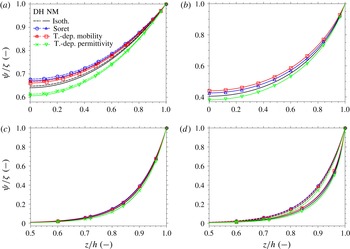
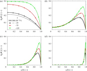
In figure 2 the relative EDL potential
 $\unicode[STIX]{x1D6F9}/\overline{\unicode[STIX]{x1D701}}=\unicode[STIX]{x1D713}/\unicode[STIX]{x1D701}$
, either affected by the intrinsic Soret effect (‘Soret’), the temperature-dependent electrophoretic mobility (‘T.-dep. mobility’) or the temperature-dependent dielectric permittivity (‘T.-dep. permittivity’), is shown. In the cases capturing the Soret effect,
 $N$
as given by (2.16) was used; otherwise
 $N=1$
. Solutions obtained with the DH approximation (given by (2.25)) are compared with the corresponding numerical solutions (‘NM’, determined by solving (2.19)) as well as with the isothermal result. The nominal Debye parameter was either
 $\overline{\unicode[STIX]{x1D705}}_{0}=1$
(a,b) or
 $\overline{\unicode[STIX]{x1D705}}_{0}=10$
(c,d), while the
 $\unicode[STIX]{x1D701}$
potential was either
 $|\unicode[STIX]{x1D701}|=15\times 10^{-3}~\text{V}$
(
 $|\overline{\unicode[STIX]{x1D701}}|\approx 0.6$
, a and c) or
 $|\unicode[STIX]{x1D701}|=125\times 10^{-3}~\text{V}$
(
 $|\overline{\unicode[STIX]{x1D701}}|\approx 5$
, b and d). For all plots,
 $\overline{S}_{0}=5\times 10^{-3}~\text{K}^{-1}$
(
 $\overline{S}_{0}T_{0}=1.49$
),
 $M_{0}=-5.1\times 10^{-3}~\text{K}^{-1}$
(
 $M_{0}T_{0}=-1.52$
) and
 $\unicode[STIX]{x0394}T=25~\text{K}$
(
 $\widehat{\unicode[STIX]{x1D6E9}}=8.39\times 10^{-2}$
) were used. Hence the plots compare the EDL potential at the channel exit (
 $x=l$
, local temperature equals
 $T=T_{0}+\unicode[STIX]{x0394}T$
) with the one at the channel entrance (
 $x=0$
,
 $T=T_{0}$
). The boundary value problem described by (2.19), respectively by (2.21), along with
 $\unicode[STIX]{x1D6F9}(\pm 1)=\pm \overline{\unicode[STIX]{x1D701}}$
at the walls, was solved by collocation with the BVP4C-function implemented in Matlab (Version 8.0.0.783, R2012b) on a Dell Precision T7500 workstation operated with Ubuntu 12.04 LTS. As verified in a grid-independence study, the solutions shown are practically indistinguishable from those obtained when the default mesh density of approximately
 $500$
grid points in the
 $Z$
-direction was reduced more than 10-fold and the default relative tolerance of
 $0.1\,\%$
was increased more than 100-fold.
Comparison of the relative EDL potential
 $\unicode[STIX]{x1D6F9}(Z)/\overline{\unicode[STIX]{x1D701}}=\unicode[STIX]{x1D713}(Z)/\unicode[STIX]{x1D701}$
for the isothermal case (‘isoth’) with the potentials obtained for cases where a temperature dependence is introduced by means of either the Soret effect (‘Soret’,
 $\overline{S}_{0}=5\times 10^{-3}~\text{K}^{-1}$
), a temperature-dependent electrophoretic mobility (‘T.-dep. mobility’) or a temperature-dependent dielectric permittivity (‘T.-dep. permittivity’,
 $M_{0}=-5.1\times 10^{-3}~\text{K}^{-1}$
). Each non-isothermal effect was analysed isolated from the others for
 $\unicode[STIX]{x0394}T=25~\text{K}$
. Within the Debye–Hückel (‘DH’) approximation, the results were computed from the analytical expressions (2.24) and (2.25), respectively, while the numerical results were obtained by solving (2.21) or (2.19) (‘NM’). The nominal Debye parameter is either
 $\overline{\unicode[STIX]{x1D705}}_{0}=1$
(a,b) or
 $\overline{\unicode[STIX]{x1D705}}_{0}=10$
(c,d); the
 $\unicode[STIX]{x1D701}$
potential is set either to
 $|\unicode[STIX]{x1D701}|=15\times 10^{-3}~\text{V}$
(a,c) or to
 $|\unicode[STIX]{x1D701}|=125\times 10^{-3}~\text{V}$
(b,d). The legend depicted in (a) is valid for (b–d) as well. In (b), the solution obtained from the DH approximation is not shown as it deviates significantly from the (more accurate) numerical solution.

For
 $\overline{\unicode[STIX]{x1D705}}_{0}=10$
and
 $\unicode[STIX]{x1D701}=15\times 10^{-3}~\text{V}$
, the DH approximations and numerical solutions agree very well. By contrast, for
 $\unicode[STIX]{x1D701}=125\times 10^{-3}~\text{V}$
the (expected) difference can be as large as
 $40\,\%$
. For
 $\overline{\unicode[STIX]{x1D705}}_{0}=1$
the well-known tendency of the DH approximation to overpredict the EDL overlap is already visible at low
 $\unicode[STIX]{x1D701}$
potentials. At
 $\unicode[STIX]{x1D701}=125\times 10^{-3}~\text{V}$
, shown in figure 2(b), the mismatch between the analytical and the (more accurate) numerical solution is too severe, so that only the numerical results are depicted. For positive values of
 $\unicode[STIX]{x0394}T$
, a temperature-dependent electrophoretic ion mobility always expands the EDL, i.e. the relative electric potential is always larger than the corresponding isothermal value at the same location. Since
 $\overline{S}_{0}$
is commonly positive, the intrinsic Soret effect typically enhances this behaviour. On the other hand, since the dielectric permittivity typically decreases with temperature, the corresponding effect reduces the relative EDL potential, i.e. it appears to shrink the EDL. In fact, if
 $$\begin{eqnarray}\displaystyle \overline{S}_{0}\approx \overline{S}_{0,eq}=-\left(\frac{1}{T_{0}}+M_{0}\right), & & \displaystyle\end{eqnarray}$$
the characteristics of the EDL are unaffected by the presence of a small thermal gradient. For an aqueous electrolyte at
 $T_{0}=298~\text{K}$
one has
 $\overline{S}_{0,eq}\approx 1.7\times 10^{-3}~\text{K}^{-1}$
. According to table 2, this is within the possible range of Soret coefficients. Thus, if not completely compensated, the effects of an intrinsic thermophoretic ion motion and a temperature-dependent electrophoretic mobility on the EDL potential are at least weakened to a comparable extent by a temperature-dependent dielectric permittivity.
As apparent from figure 2, the effect of a temperature gradient on the (relative) EDL potential
 $\unicode[STIX]{x1D6F9}/\overline{\unicode[STIX]{x1D701}}$
is relatively weak for any values of
 $\overline{\unicode[STIX]{x1D701}}$
and
 $\overline{\unicode[STIX]{x1D705}}_{0}$
. At
 $\overline{\unicode[STIX]{x1D705}}_{0}=1$
and
 $\unicode[STIX]{x1D701}=15\times 10^{-3}~\text{V}$
(shown in figure 2
a) the largest relative change of the EDL potential in comparison to isothermal conditions is approximately
 $4.6\,\%$
. At
 $\unicode[STIX]{x1D701}=125\times 10^{-3}~\text{V}$
, (shown in b) this difference is approximately
 $5.5\,\%$
. At
 $\unicode[STIX]{x1D701}=15\times 10^{-3}~\text{V}$
the increase of the relative EDL potential (compared its isothermal value) due to the intrinsic Soret effect is slightly larger than that caused by a temperature-dependent electrophoretic mobility. At
 $\unicode[STIX]{x1D701}=125\times 10^{-3}~\text{V}$
the corresponding behaviour is reversed. The same applies at
 $\overline{\unicode[STIX]{x1D705}}_{0}=10$
. For that case, the maximal change of the relative EDL potential in comparison with isothermal conditions is a little less than
 $10\,\%$
for
 $\unicode[STIX]{x1D701}=15\times 10^{-3}~\text{V}$
and approximately
 $11\,\%$
at
 $\unicode[STIX]{x1D701}=125\times 10^{-3}~\text{V}$
.
In the previous section it was argued that for
 $\unicode[STIX]{x0394}T\neq 0$
the velocity distribution (2.7) differs from the isothermal result because there may exist an axial gradient in
 $\unicode[STIX]{x1D6F9}$
. Under the condition that the
 $\unicode[STIX]{x1D701}$
potential along the channel walls is constant, an expression for
 $\unicode[STIX]{x1D6F9}$
was derived above, indicating that it is a function of the local value of the EDL thickness (described by (2.23)), which changes with
 $\widehat{\unicode[STIX]{x1D6E9}}(X)$
. Thus, indeed
 $\unicode[STIX]{x1D6F9}=f(X)$
. It can be shown that this is also the case if – instead of a constant
 $\unicode[STIX]{x1D701}$
– a constant surface charge density is assumed. Consequently, the discussed non-isothermal effects will affect the axial velocity distribution no matter whether a constant
 $\unicode[STIX]{x1D701}$
potential or a constant surface charge density along the channel wall is present.
In any case, the assumption that either the
 $\unicode[STIX]{x1D701}$
potential or the surface charge density, as well as the charges in the Stern layer, remain unaffected by the temperature gradient is to some extent questionable. However, without compromising the rigor of the present derivation, a complete treatment would also involve the temperature-dependent dissociation process of surface groups. In the supplemental material of Dietzel & Hardt (Reference Dietzel and Hardt2016) such a non-isothermal charge regulation model was developed for an aqueous electrolyte in a silicate channel, which indicated that the surface charge density appears to be only weakly affected by a non-uniform temperature. Nevertheless, employing other wall materials might give different results, about which, to the best of our knowledge, only little work is available in the literature. This is further complicated by the circumstance that many of the problem parameters are not accessible experimentally, or only in a time- and space-averaged fashion. Hence, experimentally distinguishing between these various effects is a formidable challenge. In the light of the focus of this work, these questions must be left for future investigations.
2.3 Axial velocity profile for specific
 $\unicode[STIX]{x1D6F9}$

With the knowledge of
 $\unicode[STIX]{x1D6F9}$
and
 $\unicode[STIX]{x1D6FA}$
in (2.8), the axial velocity (2.7) can be further worked out. In the
 $X$
-direction,
 $\unicode[STIX]{x1D6F9}$
and its derivatives with respect to
 $Z$
vary only with
 $\widehat{\unicode[STIX]{x1D6E9}}$
, so that
 $\unicode[STIX]{x2202}_{X}(\cdot )=\unicode[STIX]{x2202}_{\widehat{\unicode[STIX]{x1D6E9}}}(\cdot )\unicode[STIX]{x2202}_{X}\widehat{\unicode[STIX]{x1D6E9}}$
. Integrating (2.19) and using the definition of
 $\widehat{\unicode[STIX]{x1D6F9}}$
provides
 $$\begin{eqnarray}\displaystyle (\unicode[STIX]{x2202}_{Z}\unicode[STIX]{x1D6F9})^{2}=2(1+\widehat{\unicode[STIX]{x1D6E9}})^{2}\overline{\unicode[STIX]{x1D705}}^{2}[\cosh (\widehat{\unicode[STIX]{x1D6F9}})-\cosh (\widehat{\unicode[STIX]{x1D6F9}}_{c})], & & \displaystyle\end{eqnarray}$$
where, according to (2.20),
 $(1+\widehat{\unicode[STIX]{x1D6E9}})\overline{\unicode[STIX]{x1D705}}^{2}$
can be replaced by
 $\overline{\unicode[STIX]{x1D705}}_{M}^{2}N$
. The axial derivative of this equation reads
 $$\begin{eqnarray}\displaystyle \unicode[STIX]{x2202}_{X}(\unicode[STIX]{x2202}_{Z}\unicode[STIX]{x1D6F9})^{2} & = & \displaystyle (\unicode[STIX]{x2202}_{Z}\unicode[STIX]{x1D6F9})^{2}\left(\frac{1}{1+\widehat{\unicode[STIX]{x1D6E9}}}+2\frac{\unicode[STIX]{x2202}_{\widehat{\unicode[STIX]{x1D6E9}}}\overline{\unicode[STIX]{x1D705}}_{M}}{\overline{\unicode[STIX]{x1D705}}_{M}}+\frac{\unicode[STIX]{x2202}_{\widehat{\unicode[STIX]{x1D6E9}}}N}{N}\right)\unicode[STIX]{x2202}_{X}\widehat{\unicode[STIX]{x1D6E9}}\nonumber\\ \displaystyle & & \displaystyle +\,2(1+\widehat{\unicode[STIX]{x1D6E9}})\overline{\unicode[STIX]{x1D705}}_{M}^{2}N[\sinh (\widehat{\unicode[STIX]{x1D6F9}})\unicode[STIX]{x2202}_{\widehat{\unicode[STIX]{x1D6E9}}}\widehat{\unicode[STIX]{x1D6F9}}-\sinh (\widehat{\unicode[STIX]{x1D6F9}}_{c})\unicode[STIX]{x2202}_{\widehat{\unicode[STIX]{x1D6E9}}}\widehat{\unicode[STIX]{x1D6F9}}_{c}]\unicode[STIX]{x2202}_{X}\widehat{\unicode[STIX]{x1D6E9}}.\end{eqnarray}$$
With this,
 $\unicode[STIX]{x1D6FA}$
can be written as
 $$\begin{eqnarray}\displaystyle \unicode[STIX]{x1D6FA} & = & \displaystyle 2(1+\widehat{\unicode[STIX]{x1D6E9}})\overline{\unicode[STIX]{x1D705}}_{M}^{2}N\unicode[STIX]{x2202}_{X}\widehat{\unicode[STIX]{x1D6E9}}\iint [\sinh (\widehat{\unicode[STIX]{x1D6F9}})\unicode[STIX]{x2202}_{\widehat{\unicode[STIX]{x1D6E9}}}\widehat{\unicode[STIX]{x1D6F9}}-\sinh (\widehat{\unicode[STIX]{x1D6F9}}_{c})\unicode[STIX]{x2202}_{\widehat{\unicode[STIX]{x1D6E9}}}\widehat{\unicode[STIX]{x1D6F9}}_{c}]\,\text{d}^{2}Z-\unicode[STIX]{x2202}_{X}\widehat{\unicode[STIX]{x1D6E9}}\int \unicode[STIX]{x2202}_{Z}\unicode[STIX]{x1D6F9}\unicode[STIX]{x2202}_{\widehat{\unicode[STIX]{x1D6E9}}}\unicode[STIX]{x1D6F9}\,\text{d}Z\nonumber\\ \displaystyle & & \displaystyle +\left(\frac{1}{1+\widehat{\unicode[STIX]{x1D6E9}}}+\frac{\unicode[STIX]{x2202}_{\widehat{\unicode[STIX]{x1D6E9}}}N}{N}+2\frac{\unicode[STIX]{x2202}_{\widehat{\unicode[STIX]{x1D6E9}}}\overline{\unicode[STIX]{x1D705}}_{M}}{\overline{\unicode[STIX]{x1D705}}_{M}}+MT_{0}\right)\unicode[STIX]{x2202}_{X}\widehat{\unicode[STIX]{x1D6E9}}\iint (\unicode[STIX]{x2202}_{Z}\unicode[STIX]{x1D6F9})^{2}\,\text{d}^{2}Z.\end{eqnarray}$$
In the following, the derivatives with respect to
 $\widehat{\unicode[STIX]{x1D6E9}}$
need be expressed. Considering the definition of
 $\overline{\unicode[STIX]{x1D705}}_{M}$
one has
 $$\begin{eqnarray}\displaystyle \frac{\unicode[STIX]{x2202}_{\widehat{\unicode[STIX]{x1D6E9}}}\overline{\unicode[STIX]{x1D705}}_{M}}{\overline{\unicode[STIX]{x1D705}}_{M}}=-\frac{1}{2}MT_{0}, & & \displaystyle\end{eqnarray}$$
i.e. the last two terms in the round bracket of (2.29) (related to the temperature dependence of the dielectric permittivity) exactly cancel each other. Furthermore, given the definition of
 $\widehat{\unicode[STIX]{x1D6F9}}$
, one has
 $$\begin{eqnarray}\displaystyle \unicode[STIX]{x2202}_{\widehat{\unicode[STIX]{x1D6E9}}}\unicode[STIX]{x1D6F9}=(1+\widehat{\unicode[STIX]{x1D6E9}})\unicode[STIX]{x2202}_{\widehat{\unicode[STIX]{x1D6E9}}}\widehat{\unicode[STIX]{x1D6F9}}+\widehat{\unicode[STIX]{x1D6F9}}, & & \displaystyle\end{eqnarray}$$
with
 $\unicode[STIX]{x2202}_{\widehat{\unicode[STIX]{x1D6E9}}}\widehat{\unicode[STIX]{x1D6F9}}=\unicode[STIX]{x2202}_{\overline{\unicode[STIX]{x1D705}}}\widehat{\unicode[STIX]{x1D6F9}}\unicode[STIX]{x2202}_{\widehat{\unicode[STIX]{x1D6E9}}}\overline{\unicode[STIX]{x1D705}}+\unicode[STIX]{x2202}_{\widehat{\overline{\unicode[STIX]{x1D701}}}}\widehat{\unicode[STIX]{x1D6F9}}\unicode[STIX]{x2202}_{\widehat{\unicode[STIX]{x1D6E9}}}\widehat{\overline{\unicode[STIX]{x1D701}}}$
and
 $\unicode[STIX]{x2202}_{\widehat{\unicode[STIX]{x1D6E9}}}\widehat{\overline{\unicode[STIX]{x1D701}}}=-\widehat{\overline{\unicode[STIX]{x1D701}}}/(1+\widehat{\unicode[STIX]{x1D6E9}})$
. Thus
 $$\begin{eqnarray}\displaystyle \unicode[STIX]{x2202}_{\widehat{\unicode[STIX]{x1D6E9}}}\widehat{\unicode[STIX]{x1D6F9}}=\unicode[STIX]{x2202}_{\overline{\unicode[STIX]{x1D705}}}\widehat{\unicode[STIX]{x1D6F9}}\unicode[STIX]{x2202}_{\widehat{\unicode[STIX]{x1D6E9}}}\overline{\unicode[STIX]{x1D705}}-\frac{\widehat{\overline{\unicode[STIX]{x1D701}}}}{1+\widehat{\unicode[STIX]{x1D6E9}}}\unicode[STIX]{x2202}_{\widehat{\overline{\unicode[STIX]{x1D701}}}}\widehat{\unicode[STIX]{x1D6F9}} & & \displaystyle\end{eqnarray}$$
and
 $$\begin{eqnarray}\displaystyle \unicode[STIX]{x2202}_{\widehat{\unicode[STIX]{x1D6E9}}}\unicode[STIX]{x1D6F9}=(1+\widehat{\unicode[STIX]{x1D6E9}})\unicode[STIX]{x2202}_{\overline{\unicode[STIX]{x1D705}}}\widehat{\unicode[STIX]{x1D6F9}}\unicode[STIX]{x2202}_{\widehat{\unicode[STIX]{x1D6E9}}}\overline{\unicode[STIX]{x1D705}}-\widehat{\overline{\unicode[STIX]{x1D701}}}\unicode[STIX]{x2202}_{\widehat{\overline{\unicode[STIX]{x1D701}}}}\widehat{\unicode[STIX]{x1D6F9}}+\widehat{\unicode[STIX]{x1D6F9}}. & & \displaystyle\end{eqnarray}$$
Moreover, with the definition of
 $\overline{\unicode[STIX]{x1D705}}$
one has
 $$\begin{eqnarray}\displaystyle \frac{\unicode[STIX]{x2202}_{\widehat{\unicode[STIX]{x1D6E9}}}\overline{\unicode[STIX]{x1D705}}}{\overline{\unicode[STIX]{x1D705}}}=-\frac{1}{2}\left(\frac{1}{1+\widehat{\unicode[STIX]{x1D6E9}}}+MT_{0}-\frac{\unicode[STIX]{x2202}_{\widehat{\unicode[STIX]{x1D6E9}}}N}{N}\right). & & \displaystyle\end{eqnarray}$$
In the case that the redistribution of ions in the electroneutral area is approximated by the Soret equilibrium, expression (2.16) provides
 $$\begin{eqnarray}\displaystyle \frac{\unicode[STIX]{x2202}_{\widehat{\unicode[STIX]{x1D6E9}}}N}{N}=-\overline{S}_{0}T_{0}. & & \displaystyle\end{eqnarray}$$
An analytical solution exists for equations of the form (2.19), which is well described in the literature (Burgreen & Nakache Reference Burgreen and Nakache1964; Levine et al.
Reference Levine, Marriott and Robinson1975; Keh & Tseng Reference Keh and Tseng2001). From this, it is in principal possible to find analytical expressions for
 $\unicode[STIX]{x2202}_{\overline{\unicode[STIX]{x1D705}}}\widehat{\unicode[STIX]{x1D6F9}}$
and
 $\unicode[STIX]{x2202}_{\widehat{\overline{\unicode[STIX]{x1D701}}}}\widehat{\unicode[STIX]{x1D6F9}}$
. However, in the analytical solution
 $\widehat{\unicode[STIX]{x1D6F9}}$
is given implicitly, involving an incomplete elliptic integral of the first kind (Langmuir Reference Langmuir1938). In preliminary tests utilizing standard Matlab routines it was seen that this implicit character impedes obtaining
 $\widehat{\unicode[STIX]{x1D6F9}}$
in a reliable fashion, especially at larger values of
 $\overline{\unicode[STIX]{x1D705}}_{0}$
. Therefore, in practice, it is preferable to evaluate these gradients numerically. To this end, (2.19) is solved numerically for several values of
 $\overline{\unicode[STIX]{x1D705}}=\overline{\unicode[STIX]{x1D705}}_{w}$
in the vicinity of a mean value
 $\overline{\unicode[STIX]{x1D705}}_{\ast }$
, where the difference
 $\overline{\unicode[STIX]{x1D705}}_{w}-\overline{\unicode[STIX]{x1D705}}_{\ast }=\pm w\unicode[STIX]{x0394}\overline{\unicode[STIX]{x1D705}}$
is a multiple
 $w$
of a small increment
 $\unicode[STIX]{x0394}\overline{\unicode[STIX]{x1D705}}\ll 1$
. For instance (and for simplicity), the derivative
 $\unicode[STIX]{x2202}_{\overline{\unicode[STIX]{x1D705}}}\widehat{\unicode[STIX]{x1D6F9}}$
can be approximated by a finite-difference scheme, using the discrete values of
 $\widehat{\unicode[STIX]{x1D6F9}}(Z)_{|\overline{\unicode[STIX]{x1D705}}_{w}}$
obtained in the previous step. An equivalent strategy can be followed to obtain a numerical approximation of
 $\unicode[STIX]{x2202}_{\widehat{\overline{\unicode[STIX]{x1D701}}}}\widehat{\unicode[STIX]{x1D6F9}}$
.
In the case that the EDL potential is so small that the DH approximation holds,
 $\unicode[STIX]{x1D6F9}^{(DH)}$
is given by (2.25). In this case, (2.32) and (2.33), respectively, can be simplified to read
 $$\begin{eqnarray}\displaystyle \unicode[STIX]{x2202}_{\widehat{\unicode[STIX]{x1D6E9}}}\widehat{\unicode[STIX]{x1D6F9}}^{(DH)}=\unicode[STIX]{x2202}_{\overline{\unicode[STIX]{x1D705}}}\widehat{\unicode[STIX]{x1D6F9}}^{(DH)}\unicode[STIX]{x2202}_{\widehat{\unicode[STIX]{x1D6E9}}}\overline{\unicode[STIX]{x1D705}}-\frac{\widehat{\unicode[STIX]{x1D6F9}}^{(DH)}}{1+\widehat{\unicode[STIX]{x1D6E9}}} & & \displaystyle\end{eqnarray}$$
and
 $$\begin{eqnarray}\displaystyle \unicode[STIX]{x2202}_{\widehat{\unicode[STIX]{x1D6E9}}}\unicode[STIX]{x1D6F9}^{(DH)}=(1+\widehat{\unicode[STIX]{x1D6E9}})\unicode[STIX]{x2202}_{\overline{\unicode[STIX]{x1D705}}}\widehat{\unicode[STIX]{x1D6F9}}^{(DH)}\unicode[STIX]{x2202}_{\widehat{\unicode[STIX]{x1D6E9}}}\overline{\unicode[STIX]{x1D705}}=\unicode[STIX]{x2202}_{\overline{\unicode[STIX]{x1D705}}}\unicode[STIX]{x1D6F9}^{(DH)}\unicode[STIX]{x2202}_{\widehat{\unicode[STIX]{x1D6E9}}}\overline{\unicode[STIX]{x1D705}}, & & \displaystyle\end{eqnarray}$$
where
 $$\begin{eqnarray}\displaystyle \frac{\unicode[STIX]{x2202}_{\overline{\unicode[STIX]{x1D705}}}\widehat{\unicode[STIX]{x1D6F9}}^{(DH)}}{\widetilde{\overline{\unicode[STIX]{x1D701}}}}=\frac{\unicode[STIX]{x2202}_{\overline{\unicode[STIX]{x1D705}}}\unicode[STIX]{x1D6F9}^{(DH)}}{\overline{\unicode[STIX]{x1D701}}}=\frac{\cosh (\overline{\unicode[STIX]{x1D705}}Z)}{\cosh (\overline{\unicode[STIX]{x1D705}})}[\tanh (\overline{\unicode[STIX]{x1D705}}Z)Z-\tanh (\overline{\unicode[STIX]{x1D705}})]. & & \displaystyle\end{eqnarray}$$
In appendix B, the numerical evaluations of the partial derivatives
 $\unicode[STIX]{x2202}_{\overline{\unicode[STIX]{x1D705}}}\unicode[STIX]{x1D6F9}(Z)$
and
 $\unicode[STIX]{x2202}_{\widehat{\overline{\unicode[STIX]{x1D701}}}}\widehat{\unicode[STIX]{x1D6F9}}(Z)$
are further discussed. Results are presented for several values of the nominal Debye parameter and compared with solutions obtained from the DH approximation. It is shown that
 $\unicode[STIX]{x2202}_{\widehat{\unicode[STIX]{x1D6E9}}}\unicode[STIX]{x1D6F9}$
takes significant values only inside the EDL, i.e. in the non-electroneutral portion of the channel.
Within the DH approximation, after some algebra, one finds for the
 $\unicode[STIX]{x1D6FA}$
-integral expressed by (2.8)
 $$\begin{eqnarray}\displaystyle \unicode[STIX]{x1D6FA}^{(DH)} & = & \displaystyle -\frac{\overline{\unicode[STIX]{x1D701}}^{2}\unicode[STIX]{x2202}_{X}\widehat{\unicode[STIX]{x1D6E9}}}{8\cosh ^{2}(\overline{\unicode[STIX]{x1D705}})}\left\{\left[\frac{1}{2}\cosh (2\overline{\unicode[STIX]{x1D705}}Z)-\overline{\unicode[STIX]{x1D705}}^{2}Z^{2}+2\overline{\unicode[STIX]{x1D705}}^{3}Z^{2}\tanh (\overline{\unicode[STIX]{x1D705}})\right]\left(\frac{1}{1+\widehat{\unicode[STIX]{x1D6E9}}}-\frac{\unicode[STIX]{x2202}_{\widehat{\unicode[STIX]{x1D6E9}}}N}{N}\right)\right.\nonumber\\ \displaystyle & & \displaystyle \left.-\,\left[\frac{1}{2}\cosh (2\overline{\unicode[STIX]{x1D705}}Z)-\overline{\unicode[STIX]{x1D705}}^{2}Z^{2}-2\overline{\unicode[STIX]{x1D705}}^{3}Z^{2}\tanh (\overline{\unicode[STIX]{x1D705}})\right]MT_{0}\right\}.\end{eqnarray}$$
Employing (2.7), with
 $\unicode[STIX]{x2202}_{Z}\unicode[STIX]{x1D6FA}_{c}=0$
(symmetry), the axial velocity distribution reads
 $$\begin{eqnarray}\displaystyle U^{(DH)} & = & \displaystyle -\frac{\unicode[STIX]{x2202}_{X}P_{0}}{2\overline{\unicode[STIX]{x1D702}}}(1-Z^{2})+\frac{Ha\overline{\unicode[STIX]{x1D701}}}{\overline{\unicode[STIX]{x1D702}}\hspace{1.7pt}\overline{\unicode[STIX]{x1D705}}_{M}^{2}}\overline{E}\left[\frac{\cosh (\overline{\unicode[STIX]{x1D705}}Z)}{\cosh (\overline{\unicode[STIX]{x1D705}})}-1\right]-\frac{Ha}{\overline{\unicode[STIX]{x1D702}}\hspace{1.7pt}\overline{\unicode[STIX]{x1D705}}_{M}^{2}}\frac{\overline{\unicode[STIX]{x1D701}}^{2}\unicode[STIX]{x2202}_{X}\widehat{\unicode[STIX]{x1D6E9}}}{8\cosh ^{2}(\overline{\unicode[STIX]{x1D705}})}\nonumber\\ \displaystyle & & \displaystyle \times \,\left\{\left[\frac{\cosh (2\overline{\unicode[STIX]{x1D705}}Z)-\cosh (2\overline{\unicode[STIX]{x1D705}})}{2}+\overline{\unicode[STIX]{x1D705}}^{2}(1-Z^{2})\right]\left(\frac{1}{1+\widehat{\unicode[STIX]{x1D6E9}}}-\frac{\unicode[STIX]{x2202}_{\widehat{\unicode[STIX]{x1D6E9}}}N}{N}-MT_{0}\right)\right.\nonumber\\ \displaystyle & & \displaystyle \left.-\,2\overline{\unicode[STIX]{x1D705}}^{3}(1-Z^{2})\tanh (\overline{\unicode[STIX]{x1D705}})\left(\frac{1}{1+\widehat{\unicode[STIX]{x1D6E9}}}-\frac{\unicode[STIX]{x2202}_{\widehat{\unicode[STIX]{x1D6E9}}}N}{N}+MT_{0}\right)\right\}.\end{eqnarray}$$
Expression (2.40) describes the axial velocity profile across the channel if, apart from axial gradients in pressure and an induced electric potential, a thermal gradient is present along the channel as well. This gradient may cause contributions to the axial velocity due to the temperature dependencies of the electrophoretic mobility and the permittivity, as well as due to an axial gradient in salt concentration. In the latter case,
 $\unicode[STIX]{x2202}_{\widehat{\unicode[STIX]{x1D6E9}}}N$
can be expressed by (2.35) if the concentration gradient develops in accordance with the Soret equilibrium. The expressions are applicable to any type of electrokinetic flow (electroosmotic pumping or generation of an induced streaming potential by pressure-driven flow) in a slit channel.
For experimental validation, it is commonly more feasible to measure the overall volumetric flow rate
 $\dot{V}$
in a channel. Within the DH limit, integration of (2.40) across the channel width and expressing the non-dimensional parameters by their dimensional counterparts (except for
 $\overline{\unicode[STIX]{x1D705}}=\unicode[STIX]{x1D705}h$
) provides
 $$\begin{eqnarray}\displaystyle \frac{\dot{V}^{(DH)}}{2h\unicode[STIX]{x0394}y} & = & \displaystyle -\frac{h^{2}}{3\unicode[STIX]{x1D702}}\unicode[STIX]{x2202}_{x}p_{0}+\frac{\unicode[STIX]{x1D716}\unicode[STIX]{x1D701}}{\unicode[STIX]{x1D702}}E\left[\frac{\tanh (\overline{\unicode[STIX]{x1D705}})}{\overline{\unicode[STIX]{x1D705}}}-1\right]\nonumber\\ \displaystyle & & \displaystyle -\,\frac{\unicode[STIX]{x1D716}\unicode[STIX]{x1D701}^{2}}{16\unicode[STIX]{x1D702}}\unicode[STIX]{x2202}_{x}T\left\{\left[\frac{\tanh (\overline{\unicode[STIX]{x1D705}})}{\overline{\unicode[STIX]{x1D705}}}-1-\tanh ^{2}(\overline{\unicode[STIX]{x1D705}})+\frac{4}{3}\frac{\overline{\unicode[STIX]{x1D705}}^{2}}{\cosh ^{2}(\overline{\unicode[STIX]{x1D705}})}\right]\left(\frac{1}{T}-\frac{\unicode[STIX]{x2202}_{T}n}{n}-\frac{\unicode[STIX]{x1D716}_{T}}{\unicode[STIX]{x1D716}}\right)\right.\nonumber\\ \displaystyle & & \displaystyle \left.-\,\frac{8}{3}\frac{\overline{\unicode[STIX]{x1D705}}^{3}\tanh (\overline{\unicode[STIX]{x1D705}})}{\cosh ^{2}(\overline{\unicode[STIX]{x1D705}})}\left(\frac{1}{T}-\frac{\unicode[STIX]{x2202}_{T}n}{n}+\frac{\unicode[STIX]{x1D716}_{T}}{\unicode[STIX]{x1D716}}\right)\right\},\end{eqnarray}$$
where
 $\unicode[STIX]{x0394}y$
denotes the extension of the channel in the
 $y$
-direction. If the salinity varies with temperature according to the Soret equilibrium (2.35), then
 $\unicode[STIX]{x2202}_{T}n/n\equiv \unicode[STIX]{x2202}_{\widehat{\unicode[STIX]{x1D6E9}}}N/(NT_{0})=-\overline{S}_{0}$
.
2.3.1 Thermoosmotic fluid propulsion
In isothermal electrokinetic flow through channels, the advective fluid motion described by
 $U$
(or
 $U^{(DH)}$
, respectively) is driven either by an externally applied pressure gradient or an externally applied electric field. However, under the present assumptions and non-isothermal conditions (
 $\unicode[STIX]{x2202}_{X}\widehat{\unicode[STIX]{x1D6E9}}\neq 0$
), an axial advection is – counterintuitively – present even without a pressure difference (
 $\unicode[STIX]{x2202}_{X}P_{0}=0$
) and without an external field (
 $\overline{E}=0$
).
Figure 3(a) illustrates the (dimensional) axial velocity profile
 $u^{(DH)}(z)$
given by (2.40) (valid within the limits of the DH approximation) for
 $\unicode[STIX]{x0394}T=25~\text{K}$
, while
 $\unicode[STIX]{x2202}_{X}P_{0}=\overline{E}=0$
. The
 $\unicode[STIX]{x1D701}$
potential is set to
 $\unicode[STIX]{x1D701}=-25\times 10^{-3}~\text{V}$
. The nominal Debye parameter equals one of the following values:
 $\overline{\unicode[STIX]{x1D705}}_{0}=\unicode[STIX]{x1D705}_{0}h=[1,2,3,5,10]$
. Since
 $u(z)$
is proportional to the inverse of the channel length
 $l$
(not explicitly given herein), in figure 3 the ratio
 $u(z)/v_{D}$
is shown, where
 $v_{D}=D_{0}/l$
is an axial diffusion speed with the Fickian diffusion coefficient set to
 $D_{0}=10^{-9}~\text{m}^{2}~\text{s}^{-1}$
. Thermophoretic ion motion is considered using (2.35), where
 $\overline{S}_{0}=10^{-3}~\text{K}^{-1}$
, while a temperature-dependent dielectric permittivity is included with
 $M=-5.1\times 10^{-3}~\text{K}^{-1}$
. From this plot it is apparent that the maximal thermoosmotic velocity is still two to three orders of magnitude smaller than the diffusion speed. For instance, for a channel length given by
 $l=\overline{\unicode[STIX]{x1D705}}_{0}/A\unicode[STIX]{x1D705}_{0}$
with
 $\overline{\unicode[STIX]{x1D705}}_{0}=1$
,
 $A=0.1$
and
 $\unicode[STIX]{x1D705}_{0}^{-1}\approx 10^{-7}~\text{m}$
(i.e.
 $l\approx 10^{-6}~\text{m}$
) one obtains
 $u(z)\lesssim 10^{-5}~\text{m}~\text{s}^{-1}$
.
At a casual glance, the velocity profiles plotted in figure 3(a) look similar to typical profiles obtained for electroosmotic flow, resembling a plug-like structure for larger values of
 $\overline{\unicode[STIX]{x1D705}}_{0}$
. However, despite being not clearly visible on the scale of the plot, the largest velocity of thermal origin does not necessarily develop along the channel centre plane at
 $z=0$
. Rather than that, for sufficiently small
 $\overline{\unicode[STIX]{x1D705}}_{0}$
, one can estimate the location of the axial velocity peak to occur at
 $$\begin{eqnarray}\displaystyle \frac{z}{h}\approx \sqrt{-3\frac{\tanh (\overline{\unicode[STIX]{x1D705}}_{0})}{\overline{\unicode[STIX]{x1D705}}_{0}}\frac{1+MT_{0}-\unicode[STIX]{x2202}_{\widehat{\unicode[STIX]{x1D6E9}}}N/N}{1-MT_{0}-\unicode[STIX]{x2202}_{\widehat{\unicode[STIX]{x1D6E9}}}N/N}}. & & \displaystyle\end{eqnarray}$$
Since typically
 $M<0$
and
 $\unicode[STIX]{x2202}_{\widehat{\unicode[STIX]{x1D6E9}}}N/N<0$
, this equation has a real solution
 $0<z/h<1$
only if the temperature dependence of the dielectric permittivity is sufficiently strong. Thus, this dependence causes the development of a double velocity maximum in the slit channel. For instance, for the cases shown one finds
 $[\overline{\unicode[STIX]{x1D705}}_{0},z/h]\approx [1,0.43]$
,
 $[2,0.34]$
,
 $[3,0.28]$
,
 $[5,0.22]$
and
 $[10,0.16]$
(accurate solution obtained by a fix-point iteration are
 $[1,0.42]$
,
 $[2,0.33]$
,
 $[3,0.27]$
,
 $[5,0.20]$
and
 $[10,0.13]$
). Hence, for increasing
 $\overline{\unicode[STIX]{x1D705}}_{0}$
, the location of the velocity maximum approaches the channel centre plane.
Illustration of thermoosmotic fluid propulsion. (a) Thermoosmotic axial velocity profile
 $u^{(DH)}(z)$
, expressed by (2.40) relative to the axial diffusion speed
 $D_{0}/l$
(Fickian diffusion coefficient is set to
 $D_{0}=10^{-9}~\text{m}^{2}~\text{s}^{-1}$
), for the nominal Debye parameters
 $\overline{\unicode[STIX]{x1D705}}_{0}=\unicode[STIX]{x1D705}_{0}h=[1,2,3,5,10]$
,
 $\unicode[STIX]{x1D701}$
potential
 $\unicode[STIX]{x1D701}=-25\times 10^{-3}~\text{V}$
and
 $\unicode[STIX]{x0394}T=25~\text{K}$
. No external pressure gradient or external electric field is applied (
 $\unicode[STIX]{x2202}_{X}P_{0}=\overline{E}=0$
). The thermophoretic ion motion is considered by (2.35) and
 $\overline{S}_{0}=10^{-3}~\text{K}^{-1}$
, while the temperature-dependent dielectric permittivity is included with
 $M=-5.1\times 10^{-3}~\text{K}^{-1}$
. (b) Hypothetical case, where only the temperature dependence of the dielectric permittivity is included (
 $M=-5.1\times 10^{-3}~\text{K}^{-1}$
), whereas thermophoretic ion motion and a temperature-dependent ion mobility are absent. (c) Volumetric flow rate
 $\dot{V}^{(DH)}$
expressed by (2.41), scaled to
 $2h\unicode[STIX]{x0394}yD_{0}/l$
, and plotted as a function of
 $\overline{\unicode[STIX]{x1D705}}_{0}$
for a temperature difference of
 $\unicode[STIX]{x0394}T=5$
,
 $15$
and
 $25~\text{K}$
. All other conditions and parameters are identical to those used in (a).

This effect can be enhanced by (artificially) eliminating the thermophoretic ion motion and the temperature dependence of the ion mobility altogether. The velocity profiles for this (hypothetical) case are shown in figure 3(b) for the same parameter values as depicted in (a). Here, the deviation from the single maximum profile is especially visible for smaller values of
 $\overline{\unicode[STIX]{x1D705}}_{0}$
. For
 $\overline{\unicode[STIX]{x1D705}}_{0}=2$
, the axial flow even switches direction as a function of
 $z$
, i.e. it is in one direction close to the wall and in the opposite direction close to the channel centre plane. For
 $\overline{\unicode[STIX]{x1D705}}_{0}=1$
, the axial flow is opposite to the one observed for larger values of
 $\overline{\unicode[STIX]{x1D705}}_{0}$
throughout the channel cross-section. The reason for this behaviour lies in the multitude of mechanisms to which a temperature-dependent dielectric permittivity contributes: firstly, it adds an extra source term to the Maxwell stresses in the Navier–Stokes equation. Secondly, it alters the electrohydrodynamic pressure of the ions and lastly, it modifies the Poisson equation. The latter has direct implications for the specific form of the EDL potential.
In figure 3(c) the volumetric flow rate
 $\dot{V}$
in the DH limit as given by (2.41) and scaled to
 $2h\unicode[STIX]{x0394}yD_{0}/l$
is plotted as a function of
 $\overline{\unicode[STIX]{x1D705}}_{0}$
for a temperature difference of
 $\unicode[STIX]{x0394}T=5$
,
 $15$
, and
 $25~\text{K}$
. The other parameters are identical to those of figure 3(a), in particular
 $\unicode[STIX]{x2202}_{X}P_{0}=\overline{E}=0$
as well. After a steep increase within
 $1\lesssim \overline{\unicode[STIX]{x1D705}}_{0}\lesssim 3$
, it is found that
 $\dot{V}^{(DH)}$
quickly saturates to
 $$\begin{eqnarray}\displaystyle \frac{1}{2h\unicode[STIX]{x0394}yD_{0}}\left(\frac{\dot{V}}{\unicode[STIX]{x2202}_{x}T}\right)_{|\overline{\unicode[STIX]{x1D705}}_{0}\rightarrow \infty }^{(DH)}=\frac{\unicode[STIX]{x1D716}\unicode[STIX]{x1D701}^{2}}{8\unicode[STIX]{x1D702}D_{0}}\left(\frac{1}{T}-\frac{\unicode[STIX]{x2202}_{T}n}{n}-\frac{\unicode[STIX]{x1D716}_{T}}{\unicode[STIX]{x1D716}}\right), & & \displaystyle\end{eqnarray}$$
when
 $\overline{\unicode[STIX]{x1D705}}_{0}\gtrsim 10$
and for all
 $\unicode[STIX]{x0394}T$
(
 $\unicode[STIX]{x2202}_{x}T=\unicode[STIX]{x0394}T/l$
). For the parameter set used in figure 3, (2.43) equals
 $5.8\times 10^{-4}~\text{K}^{-1}$
.
EDL potential
 $\unicode[STIX]{x1D713}(x,z)/\unicode[STIX]{x1D701}$
in the channel for the case of thermophoretic ion motion due to Soret A alone, i.e. both ion species have the same thermophoretic mobility. The nominal Debye parameter is
 $\overline{\unicode[STIX]{x1D705}}_{0}=8$
and, for illustrative purposes,
 $S\unicode[STIX]{x0394}T=2.5$
was chosen (plot is exaggerated). Inset: effective axial body force density (2.44) due to the interaction of the ion cloud with the charges at the wall boundaries. The externally applied pressure gradient and the induced field are absent (
 $\unicode[STIX]{x2202}_{X}P_{0}=\overline{E}=0$
).

The origin of the observed fluid propulsion if only a thermal gradient is present needs some further explanation. If
 $\unicode[STIX]{x2202}_{X}\widehat{\unicode[STIX]{x1D6E9}}\neq 0$
, the EDL thickness varies along the channel, i.e. the EDL potential becomes dependent on the axial coordinate. In figure 4 this is shown schematically for the special case of identical thermophoretic mobilities of the ion species. In the following, we will refer to this special form of thermophoretic ion motion as type Soret A ion thermodiffusion. By contrast, thermally induced ion motion where only one ion species moves within a temperature gradient will be referred to as Soret B ion thermodiffusion. In figure 4, for illustrative purposes,
 $S_{0}\unicode[STIX]{x0394}T=2.5$
was chosen (Soret A), i.e. the plot is exaggerated. The nominal Debye parameter is set to
 $\overline{\unicode[STIX]{x1D705}}_{0}=8$
. The combination of the (weak) modification of the EDL along the axial coordinate
 $X$
with the steep lateral gradient of
 $\unicode[STIX]{x1D6F9}$
inside the EDL leads to an axial electric field confined to the EDL only, see appendix B. In turn, this field causes an axial gradient in the electrohydrostatic pressure (being equivalent to the osmotic pressure gradient
 $-k_{B}T\unicode[STIX]{x2202}_{x}n$
, where
 $n=\sum _{k=1}^{K}n_{k}$
) as well as an axial electromotive body force
 $-\unicode[STIX]{x1D70C}_{f}\unicode[STIX]{x2202}_{x}\unicode[STIX]{x1D713}$
(excluding for simplicity the contributions from a temperature-dependent dielectric permittivity), which only partially cancel each other. Hence, by contrast to isothermal conditions, the ion cloud is not necessarily in mechanical equilibrium. Instead, as shown in appendix C (expression (C 13)), a net force density acts on the excess ions in the EDL. Using (2.35), this force density can be described by
 $$\begin{eqnarray}\displaystyle \frac{F_{EDL,x}}{k_{B}T_{0}n_{0}\unicode[STIX]{x2202}_{x}\widehat{\unicode[STIX]{x1D6E9}}}\approx 2\{[\cosh (\unicode[STIX]{x1D6F9}^{(e)})-1]S_{0}T_{0}+\unicode[STIX]{x1D6F9}^{(e)}\sinh (\unicode[STIX]{x1D6F9}^{(e)})\}. & & \displaystyle\end{eqnarray}$$
The first term in the curly bracket on the right-hand side expresses the contribution by the thermophoretic ion motion, while the second describes the thermomechanical effect of a temperature-dependent ion mobility. In this linearized form,
 $F_{EDL,x}$
does not vary along the channel centre plane and is plotted in the inset of figure 4. As detailed in appendix C, this force density does not appear to be an artefact of the lubrication approximation or the specific scaling used in the present derivation. Being proportional to the axial temperature gradient,
 $F_{EDL,x}$
vanishes if the temperature is uniform. Hence, under isothermal conditions, the EDL field itself cannot propel the surrounding fluid.
Essentially, regardless of the physical origin, any modification of the EDL causing an imbalance between the electromotive and the osmotic pressure should lead to a similar effect. For instance, the essential difference of this work compared to that of Sasidhar & Ruckenstein (Reference Sasidhar and Ruckenstein1982) is that in the latter an axial concentration gradient is applied externally as an independent parameter, while here, it is caused by the axial temperature gradient. For large
 $\overline{\unicode[STIX]{x1D705}}_{0}\rightarrow \infty$
, the corresponding fluid motion may be regarded as a thermally induced, apparent double layer slip velocity.
As detailed in the following sections, the thermoosmotic flux driven by a mechanical imbalance of the ion cloud in the EDL as described here also contributes to the induced electric field. It should be emphasized that, in this study, the incorporation of the Korteweg–Helmholtz electric force in the momentum equation is of crucial importance; otherwise the described phenomenon cannot be correctly captured. This distinguishes this study from common considerations of isothermal electrokinetics where the force term is not necessary to compute the streaming potential, but is merely included to predict the (commonly weak) electroosmotic flow, opposing the pressure-induced flow, and to fulfil the Onsager reciprocal condition.
2.4 Electric currents and induced potential
Besides the EDL potential derived in § 2.2, an induced or externally applied potential may be present, which does not affect the local charge density. In studies of pressure-driven systems kept at uniform temperature, the induced potential is identical to the so-called streaming potential and can be determined by multiplying (2.15) by
 $\overline{\unicode[STIX]{x1D708}}_{k}$
, summing over all ion species, integrating across the channel section and setting the result equal to zero. Applying the same procedure to the system considered here results in
 $$\begin{eqnarray}\displaystyle & & \displaystyle -\frac{\overline{E}}{1+\widehat{\unicode[STIX]{x1D6E9}}}\int _{0}^{1}\mathop{\sum }_{k=1}^{K}\frac{\overline{\unicode[STIX]{x1D708}}_{k}^{2}N_{k}}{Pe_{k}}\,\text{d}Z+\frac{\unicode[STIX]{x2202}_{X}\widehat{\unicode[STIX]{x1D6E9}}}{(1+\widehat{\unicode[STIX]{x1D6E9}})^{2}}\int _{0}^{1}\unicode[STIX]{x1D6F9}\mathop{\sum }_{k=1}^{K}\frac{\overline{\unicode[STIX]{x1D708}}_{k}^{2}N_{k}}{Pe_{k}}\,\text{d}Z\nonumber\\ \displaystyle & & \displaystyle \quad +\,T_{0}\unicode[STIX]{x2202}_{X}\widehat{\unicode[STIX]{x1D6E9}}\int _{0}^{1}\mathop{\sum }_{k=1}^{K}\frac{\overline{\unicode[STIX]{x1D708}}_{k}N_{k}S_{k}}{Pe_{k}}\,\text{d}Z\nonumber\\ \displaystyle & & \displaystyle \quad +\,\frac{\unicode[STIX]{x2202}_{X}N}{N}\int _{0}^{1}\mathop{\sum }_{k=1}^{K}\frac{\overline{\unicode[STIX]{x1D708}}_{k}N_{k}}{Pe_{k}}\,\text{d}Z=\int _{0}^{1}U\mathop{\sum }_{k=1}^{K}\overline{\unicode[STIX]{x1D708}}_{k}N_{k}\,\text{d}Z.\end{eqnarray}$$
2.4.1 Streaming current
When integrated over the extension of the channel in the
 $y$
-direction
 $\unicode[STIX]{x0394}y$
, the term on the right-hand side of (2.45) represents the total streaming current
 $I_{st}=2\unicode[STIX]{x0394}y\int _{0}^{h}\unicode[STIX]{x1D70C}_{f}u\,\text{d}z$
. According to the leading-order terms in (2.2), the charge density
 $\unicode[STIX]{x1D70C}_{f}/(e\unicode[STIX]{x1D708}n_{0})=\sum _{k=1}^{K}\overline{\unicode[STIX]{x1D708}}_{k}N_{k}$
is equal to
 $-2/(\overline{\unicode[STIX]{x1D705}}_{M}^{2})\unicode[STIX]{x2202}_{Z}^{2}\unicode[STIX]{x1D6F9}$
. Integrating by parts under the given boundary conditions leads to
 $I_{st}/(2\unicode[STIX]{x0394}yu_{0}e\unicode[STIX]{x1D708}n_{0})=2/\overline{\unicode[STIX]{x1D705}}_{M}^{2}\int _{0}^{1}\unicode[STIX]{x2202}_{Z}U\unicode[STIX]{x2202}_{Z}\unicode[STIX]{x1D6F9}\,\text{d}Z$
. With an expression for
 $\unicode[STIX]{x2202}_{Z}U$
derived from (2.7), this leads to
 $$\begin{eqnarray}\displaystyle \frac{I_{st}\unicode[STIX]{x1D708}e}{2\unicode[STIX]{x0394}y\unicode[STIX]{x1D705}_{M}u_{0}\unicode[STIX]{x1D716}k_{B}T_{0}}=\overline{I}_{st,P}\unicode[STIX]{x2202}_{X}P_{0}-\overline{I}_{st,\overline{E}}\overline{E}+\overline{I}_{st,\unicode[STIX]{x1D6E9}}\unicode[STIX]{x2202}_{X}\unicode[STIX]{x1D6E9}, & & \displaystyle\end{eqnarray}$$
where
 $$\begin{eqnarray}\displaystyle \left.\begin{array}{@{}c@{}}\displaystyle \overline{I}_{st,P}=\frac{1}{\overline{\unicode[STIX]{x1D705}}_{M}\overline{\unicode[STIX]{x1D702}}}\left(\overline{\unicode[STIX]{x1D701}}-\int _{0}^{1}\unicode[STIX]{x1D6F9}\,\text{d}Z\right),\quad \overline{I}_{st,\overline{E}}=-\frac{Ha}{\overline{\unicode[STIX]{x1D705}}_{M}^{3}\overline{\unicode[STIX]{x1D702}}}\int _{0}^{1}(\unicode[STIX]{x2202}_{Z}\unicode[STIX]{x1D6F9})^{2}\,\text{d}Z,\\ \displaystyle \overline{I}_{st,\unicode[STIX]{x1D6E9}}=\frac{Ha}{\overline{\unicode[STIX]{x1D705}}_{M}^{3}\overline{\unicode[STIX]{x1D702}}}\frac{1}{\unicode[STIX]{x2202}_{X}\unicode[STIX]{x1D6E9}}\int _{0}^{1}\unicode[STIX]{x2202}_{Z}\unicode[STIX]{x1D6FA}\unicode[STIX]{x2202}_{Z}\unicode[STIX]{x1D6F9}\,\text{d}Z.\end{array}\right\} & & \displaystyle\end{eqnarray}$$
With (2.29) and (2.30), the last integral in (2.47) can be written as
 $$\begin{eqnarray}\displaystyle & & \displaystyle \int _{0}^{1}\unicode[STIX]{x2202}_{Z}\unicode[STIX]{x1D6FA}\unicode[STIX]{x2202}_{Z}\unicode[STIX]{x1D6F9}\,\text{d}Z=2(1+\widehat{\unicode[STIX]{x1D6E9}})\overline{\unicode[STIX]{x1D705}}_{M}^{2}N\unicode[STIX]{x2202}_{X}\widehat{\unicode[STIX]{x1D6E9}}\nonumber\\ \displaystyle & & \displaystyle \quad \times \,\int _{0}^{1}\unicode[STIX]{x2202}_{Z}\unicode[STIX]{x1D6F9}\left\{\int [\sinh (\widehat{\unicode[STIX]{x1D6F9}})\unicode[STIX]{x2202}_{\widehat{\unicode[STIX]{x1D6E9}}}\widehat{\unicode[STIX]{x1D6F9}}-\sinh (\widehat{\unicode[STIX]{x1D6F9}}_{c})\unicode[STIX]{x2202}_{\widehat{\unicode[STIX]{x1D6E9}}}\widehat{\unicode[STIX]{x1D6F9}}_{c}]\,\text{d}Z\right\}\text{d}Z\nonumber\\ \displaystyle & & \displaystyle \quad -\,\unicode[STIX]{x2202}_{X}\widehat{\unicode[STIX]{x1D6E9}}\int _{0}^{1}(\unicode[STIX]{x2202}_{Z}\unicode[STIX]{x1D6F9})^{2}\unicode[STIX]{x2202}_{\widehat{\unicode[STIX]{x1D6E9}}}\unicode[STIX]{x1D6F9}\,\text{d}Z+\left(\frac{1}{1+\widehat{\unicode[STIX]{x1D6E9}}}+\frac{\unicode[STIX]{x2202}_{\widehat{\unicode[STIX]{x1D6E9}}}N}{N}\right)\unicode[STIX]{x2202}_{X}\widehat{\unicode[STIX]{x1D6E9}}\int _{0}^{1}\unicode[STIX]{x2202}_{Z}\unicode[STIX]{x1D6F9}\left[\int (\unicode[STIX]{x2202}_{Z}\unicode[STIX]{x1D6F9})^{2}\,\text{d}Z\right]\text{d}Z.\nonumber\\ \displaystyle & & \displaystyle\end{eqnarray}$$
In general,
 $\widehat{\unicode[STIX]{x1D6F9}}$
is obtained by solving numerically (2.19), while
 $\unicode[STIX]{x2202}_{Z}\unicode[STIX]{x1D6F9}$
is given by (2.27). Furthermore,
 $\unicode[STIX]{x2202}_{\widehat{\unicode[STIX]{x1D6E9}}}\widehat{\unicode[STIX]{x1D6F9}}$
is obtained from (2.32) by the numerical approach outlined before, while
 $\unicode[STIX]{x2202}_{\widehat{\unicode[STIX]{x1D6E9}}}\unicode[STIX]{x1D6F9}$
is computed from (2.33). Thus, the integrals in (2.47) and (2.48) are fully described and can be evaluated numerically.
Within the DH approximation and after some algebraic manipulations, the (dimensionless) streaming current reads
 $$\begin{eqnarray}\displaystyle & & \displaystyle \frac{(I_{st})^{(DH)}\unicode[STIX]{x1D708}e}{2\unicode[STIX]{x0394}y\unicode[STIX]{x1D705}_{M}u_{0}\unicode[STIX]{x1D716}k_{B}T_{0}}=\frac{\overline{\unicode[STIX]{x1D701}}\unicode[STIX]{x2202}_{X}P_{0}}{\overline{\unicode[STIX]{x1D705}}_{M}\overline{\unicode[STIX]{x1D702}}}\left[1-\frac{\tanh (\overline{\unicode[STIX]{x1D705}})}{\overline{\unicode[STIX]{x1D705}}}\right]\nonumber\\ \displaystyle & & \displaystyle \quad +\,\frac{Ha\overline{\unicode[STIX]{x1D701}}^{2}\overline{E}}{2\overline{\unicode[STIX]{x1D705}}_{M}\overline{\unicode[STIX]{x1D702}}}\left(\frac{\overline{\unicode[STIX]{x1D705}}}{\overline{\unicode[STIX]{x1D705}}_{M}}\right)^{2}\left[\frac{\tanh (\overline{\unicode[STIX]{x1D705}})}{\overline{\unicode[STIX]{x1D705}}}-\frac{1}{\cosh ^{2}(\overline{\unicode[STIX]{x1D705}})}\right]-\frac{Ha\overline{\unicode[STIX]{x1D701}}^{3}\unicode[STIX]{x2202}_{X}\widehat{\unicode[STIX]{x1D6E9}}}{2\overline{\unicode[STIX]{x1D705}}_{M}\overline{\unicode[STIX]{x1D702}}}\left(\frac{\overline{\unicode[STIX]{x1D705}}}{\overline{\unicode[STIX]{x1D705}}_{M}}\right)^{2}\nonumber\\ \displaystyle & & \displaystyle \quad \times \left\{-\frac{\unicode[STIX]{x2202}_{\widehat{\unicode[STIX]{x1D6E9}}}N}{N}\left[\frac{\overline{\unicode[STIX]{x1D705}}\tanh (\overline{\unicode[STIX]{x1D705}})-\tanh ^{2}(\overline{\unicode[STIX]{x1D705}})-1/2}{\cosh ^{2}(\overline{\unicode[STIX]{x1D705}})}+\frac{\tanh (\overline{\unicode[STIX]{x1D705}})}{2\overline{\unicode[STIX]{x1D705}}}-\frac{\tanh ^{3}(\overline{\unicode[STIX]{x1D705}})}{3\overline{\unicode[STIX]{x1D705}}}\right]\right.\nonumber\\ \displaystyle & & \displaystyle \quad \left.+\,\frac{1}{1+\widehat{\unicode[STIX]{x1D6E9}}}\left[\frac{\overline{\unicode[STIX]{x1D705}}\tanh (\overline{\unicode[STIX]{x1D705}})-\tanh ^{2}(\overline{\unicode[STIX]{x1D705}})-1/2}{\cosh ^{2}(\overline{\unicode[STIX]{x1D705}})}+\frac{\tanh (\overline{\unicode[STIX]{x1D705}})}{2\overline{\unicode[STIX]{x1D705}}}-\frac{\tanh ^{3}(\overline{\unicode[STIX]{x1D705}})}{3\overline{\unicode[STIX]{x1D705}}}\right]\right.\nonumber\\ \displaystyle & & \displaystyle \quad \left.+\,MT_{0}\left[\frac{\overline{\unicode[STIX]{x1D705}}\tanh (\overline{\unicode[STIX]{x1D705}})-\tanh ^{2}(\overline{\unicode[STIX]{x1D705}})+1/2}{\cosh ^{2}(\overline{\unicode[STIX]{x1D705}})}-\frac{\tanh (\overline{\unicode[STIX]{x1D705}})}{2\overline{\unicode[STIX]{x1D705}}}+\frac{\tanh ^{3}(\overline{\unicode[STIX]{x1D705}})}{3\overline{\unicode[STIX]{x1D705}}}\right]\right\},\end{eqnarray}$$
where
 $$\begin{eqnarray}\displaystyle \left(\frac{\overline{\unicode[STIX]{x1D705}}}{\overline{\unicode[STIX]{x1D705}}_{M}}\right)^{2}=\frac{N}{1+\widehat{\unicode[STIX]{x1D6E9}}}. & & \displaystyle\end{eqnarray}$$
The first term in the curly bracket of (2.49) denotes the contribution due to a gradient in salt concentration, the second quantifies the contribution due the temperature dependence of the electrophoretic ion mobility and the last term accounts for the temperature-dependent dielectric permittivity.
2.4.2 Conduction current
Going back to (2.45), the left-hand side represents the conduction current
 $-I_{cd}$
. Since the temperature gradient across the channel is negligibly small, in dimensionless form
 $I_{cd}$
is given by
 $$\begin{eqnarray}\displaystyle \frac{I_{cd}e\unicode[STIX]{x1D708}}{2\unicode[STIX]{x0394}y\unicode[STIX]{x1D705}_{M}u_{0}\unicode[STIX]{x1D716}k_{B}T_{0}} & = & \displaystyle \frac{\overline{E}}{1+\widehat{\unicode[STIX]{x1D6E9}}}\frac{\overline{\unicode[STIX]{x1D705}}_{M}}{2Pe}\int _{0}^{1}\mathop{\sum }_{k=1}^{K}\overline{\unicode[STIX]{x1D708}}_{k}^{2}N_{k}\,\text{d}Z-\frac{\unicode[STIX]{x2202}_{X}\widehat{\unicode[STIX]{x1D6E9}}}{(1+\widehat{\unicode[STIX]{x1D6E9}})^{2}}\frac{\overline{\unicode[STIX]{x1D705}}_{M}}{2Pe}\int _{0}^{1}\unicode[STIX]{x1D6F9}\mathop{\sum }_{k=1}^{K}\overline{\unicode[STIX]{x1D708}}_{k}^{2}N_{k}\,\text{d}Z\nonumber\\ \displaystyle & & \displaystyle -\,T_{0}\unicode[STIX]{x2202}_{X}\widehat{\unicode[STIX]{x1D6E9}}\frac{\overline{\unicode[STIX]{x1D705}}_{M}}{2Pe}\int _{0}^{1}\mathop{\sum }_{k=1}^{K}\overline{\unicode[STIX]{x1D708}}_{k}N_{k}S_{k}\,\text{d}Z-\frac{\unicode[STIX]{x2202}_{\widehat{\unicode[STIX]{x1D6E9}}}N\unicode[STIX]{x2202}_{X}\widehat{\unicode[STIX]{x1D6E9}}}{N}\frac{\overline{\unicode[STIX]{x1D705}}_{M}}{2Pe}\int _{0}^{1}\mathop{\sum }_{k=1}^{K}\overline{\unicode[STIX]{x1D708}}_{k}N_{k}\,\text{d}Z,\nonumber\\ \displaystyle & & \displaystyle\end{eqnarray}$$
where identical (but not necessarily constant) Fickian diffusion coefficients for each ion species (i.e.
 $D_{k}\equiv D$
) are assumed. Note that this is the first time within the derivation where such an assumption is made. For symmetric electrolytes, employing (2.17), the sums can be further evaluated to read
 $$\begin{eqnarray}\displaystyle \frac{I_{cd}\unicode[STIX]{x1D708}e}{2\unicode[STIX]{x0394}y\unicode[STIX]{x1D705}_{M}u_{0}\unicode[STIX]{x1D716}k_{B}T_{0}}=-\overline{I}_{cd,\overline{E}}\overline{E}+\overline{I}_{cd,\widehat{\unicode[STIX]{x1D6E9}}}\unicode[STIX]{x2202}_{X}\widehat{\unicode[STIX]{x1D6E9}}, & & \displaystyle\end{eqnarray}$$
where
 $$\begin{eqnarray}\displaystyle \overline{I}_{cd,\overline{E}}=-\frac{N}{1+\widehat{\unicode[STIX]{x1D6E9}}}\frac{\overline{\unicode[STIX]{x1D705}}_{M}}{Pe}\int _{0}^{1}\cosh (\widehat{\unicode[STIX]{x1D6F9}})\,\text{d}Z, & & \displaystyle\end{eqnarray}$$
and
 $$\begin{eqnarray}\displaystyle \overline{I}_{cd,\widehat{\unicode[STIX]{x1D6E9}}} & = & \displaystyle -\frac{N}{1+\widehat{\unicode[STIX]{x1D6E9}}}\frac{\overline{\unicode[STIX]{x1D705}}_{M}}{Pe}\int _{0}^{1}\widehat{\unicode[STIX]{x1D6F9}}\cosh (\widehat{\unicode[STIX]{x1D6F9}})\,\text{d}Z+S_{-}T_{0}N\frac{\overline{\unicode[STIX]{x1D705}}_{M}}{Pe}\int _{0}^{1}\sinh (\widehat{\unicode[STIX]{x1D6F9}})\,\text{d}Z\nonumber\\ \displaystyle & & \displaystyle -\,\frac{1}{2}\unicode[STIX]{x0394}ST_{0}N\frac{\overline{\unicode[STIX]{x1D705}}_{M}}{Pe}\int _{0}^{1}\exp (-\widehat{\unicode[STIX]{x1D6F9}})\,\text{d}Z+\frac{\unicode[STIX]{x2202}_{\widehat{\unicode[STIX]{x1D6E9}}}N}{N}\frac{\left(\unicode[STIX]{x2202}_{Z}\unicode[STIX]{x1D6F9}\right)_{s}}{\overline{\unicode[STIX]{x1D705}}_{M}Pe}.\end{eqnarray}$$
The intrinsic Soret coefficient of the anion is denoted by
 $S_{-}$
, while
 $S_{+}$
describes the intrinsic Soret coefficient of the cation and
 $\unicode[STIX]{x0394}S=S_{+}-S_{-}$
. Note that the conduction current expressed by (2.52) still includes the temperature dependencies of the electrophoretic mobility and of the (Fickian) diffusion coefficient.
The DH approximation yields
 $$\begin{eqnarray}\displaystyle \frac{(I_{cd})^{(DH)}\unicode[STIX]{x1D708}e}{2\unicode[STIX]{x0394}y\unicode[STIX]{x1D705}_{M}u_{0}\unicode[STIX]{x1D716}k_{B}T_{0}} & = & \displaystyle \frac{\overline{E}}{Pe}\left(\frac{\overline{\unicode[STIX]{x1D705}}}{\overline{\unicode[STIX]{x1D705}}_{M}}\right)\overline{\unicode[STIX]{x1D705}}\left\{1+\frac{\overline{\unicode[STIX]{x1D701}}^{2}}{4(1+\widehat{\unicode[STIX]{x1D6E9}})^{2}}\left[\frac{\tanh (\overline{\unicode[STIX]{x1D705}})}{\overline{\unicode[STIX]{x1D705}}}+\frac{1}{\cosh ^{2}(\overline{\unicode[STIX]{x1D705}})}\right]\right\}\nonumber\\ \displaystyle & & \displaystyle -\,\frac{\unicode[STIX]{x2202}_{X}\widehat{\unicode[STIX]{x1D6E9}}}{Pe}\left(\frac{\overline{\unicode[STIX]{x1D705}}}{\overline{\unicode[STIX]{x1D705}}_{M}}\right)\overline{\unicode[STIX]{x1D705}}\left\{\frac{\overline{\unicode[STIX]{x1D701}}}{1+\widehat{\unicode[STIX]{x1D6E9}}}\frac{\tanh (\overline{\unicode[STIX]{x1D705}})}{\overline{\unicode[STIX]{x1D705}}}\right.\nonumber\\ \displaystyle & & \displaystyle +\,\frac{\overline{\unicode[STIX]{x1D701}}^{3}}{2(1+\widehat{\unicode[STIX]{x1D6E9}})^{3}}\frac{\tanh (\overline{\unicode[STIX]{x1D705}})}{\overline{\unicode[STIX]{x1D705}}}\left[\frac{\tanh ^{2}(\overline{\unicode[STIX]{x1D705}})}{3}+\frac{1}{\cosh ^{2}(\overline{\unicode[STIX]{x1D705}})}\right]\nonumber\\ \displaystyle & & \displaystyle \left.-\,\overline{\unicode[STIX]{x1D701}}\left[\frac{1}{2}(2S_{-}+\unicode[STIX]{x0394}S)T_{0}+\frac{\unicode[STIX]{x2202}_{\widehat{\unicode[STIX]{x1D6E9}}}N}{N}\right]\tanh (\overline{\unicode[STIX]{x1D705}})/\overline{\unicode[STIX]{x1D705}}+\frac{1}{2}\unicode[STIX]{x0394}ST_{0}(1+\widehat{\unicode[STIX]{x1D6E9}})\right\}.\nonumber\\ \displaystyle & & \displaystyle\end{eqnarray}$$
2.4.3 Induced electric field dominated by external pressure difference
The induced electric field must fulfil (2.45), i.e.
 $I_{st}+I_{cd}=0$
. From (2.46) and (2.52), one finds for the local (dimensionless) streaming field
 $$\begin{eqnarray}\displaystyle \overline{E}=\frac{\overline{I}_{st,P}\unicode[STIX]{x2202}_{X}P_{0}+(\overline{I}_{st,\widehat{\unicode[STIX]{x1D6E9}}}+\overline{I}_{cd,\widehat{\unicode[STIX]{x1D6E9}}})\unicode[STIX]{x2202}_{X}\widehat{\unicode[STIX]{x1D6E9}}}{\overline{I}_{st,\overline{E}}+\overline{I}_{cd,\overline{E}}}. & & \displaystyle\end{eqnarray}$$
At first, we want to consider slit channels where the induced field is mainly caused by the externally applied pressure gradient
 $\unicode[STIX]{x2202}_{x}p_{0}$
. The latter was introduced as an integration constant in the course of the derivation of (2.6), which implies that
 $p_{0}$
is not necessarily identical to the total fluid pressure. The induced field one obtains corresponds to the conventional streaming field known for isothermal systems. Hence, if the dimensionless externally applied pressure gradient is much larger than the dimensionless thermal gradient, we will refer to the induced field as the streaming field also under non-isothermal conditions. After reinserting the definitions of the dimensionless parameters to obtain dimensional values, the local streaming field per applied pressure gradient is given by
 $$\begin{eqnarray}\displaystyle \frac{E_{p}}{\unicode[STIX]{x2202}_{x}p_{0}}=\frac{k_{B}T_{0}}{e\unicode[STIX]{x1D708}}\frac{A\overline{\unicode[STIX]{x1D705}}_{0}}{\unicode[STIX]{x1D705}_{0}u_{0}\unicode[STIX]{x1D702}_{0}}\frac{\overline{E}}{\unicode[STIX]{x2202}_{X}P_{0}}, & & \displaystyle\end{eqnarray}$$
where
 $\overline{E}$
is given by (2.56) and the subscript
 $p$
added to
 $E$
marks the streaming field induced by an external pressure difference. Note that while the characteristic parameters
 $A$
and
 $u_{0}$
need to stay in a certain range so that the simplified governing equations remain valid, the value of the local streaming field expressed by (2.57) does not depend on the specific choice of these parameters. This is because the dimensionless functions
 $\overline{I}_{st,\unicode[STIX]{x1D711}}$
(
 $\unicode[STIX]{x1D711}=P_{0},\overline{E},\widehat{\unicode[STIX]{x1D6E9}}$
) and
 $\overline{I}_{cd,\unicode[STIX]{x1D71A}}$
(
 $\unicode[STIX]{x1D71A}=\overline{E},\widehat{\unicode[STIX]{x1D6E9}}$
) depend on these parameters in a reciprocal fashion (in comparison with the pre-factor) so that the specific values cancel out. This can best be verified by considering the local streaming field in the DH limit, which reads
 $$\begin{eqnarray}\displaystyle -\left(\frac{E_{p}}{\unicode[STIX]{x2202}_{x}p_{0}}\right)^{(DH)} & = & \displaystyle \left(F_{CS}+\frac{\unicode[STIX]{x1D701}^{2}}{2}\frac{\unicode[STIX]{x1D716}}{D\unicode[STIX]{x1D702}}F_{\unicode[STIX]{x1D6FC}}\right)^{-1}\left\{\frac{\unicode[STIX]{x1D701}}{\unicode[STIX]{x1D705}^{2}D\unicode[STIX]{x1D702}}\left[1-\frac{\tanh (\overline{\unicode[STIX]{x1D705}})}{\overline{\unicode[STIX]{x1D705}}}\right]\right.\nonumber\\ \displaystyle & & \displaystyle \left.+\,\frac{\unicode[STIX]{x1D701}^{3}}{2}\frac{\unicode[STIX]{x1D716}}{D\unicode[STIX]{x1D702}}\frac{\unicode[STIX]{x0394}T/T_{0}}{\unicode[STIX]{x0394}p_{0}}\frac{\unicode[STIX]{x2202}_{\widehat{\unicode[STIX]{x1D6E9}}}N}{N}\left[F_{\unicode[STIX]{x1D6FD}}-\frac{\tanh (\overline{\unicode[STIX]{x1D705}})}{\overline{\unicode[STIX]{x1D705}}}\left(\frac{\tanh ^{2}(\overline{\unicode[STIX]{x1D705}})}{3}-\frac{1}{2}\right)\right]\right.\nonumber\\ \displaystyle & & \displaystyle \left.-\,\frac{\unicode[STIX]{x1D701}^{3}}{2}\frac{\unicode[STIX]{x1D716}}{D\unicode[STIX]{x1D702}}\frac{\unicode[STIX]{x0394}T/T_{0}}{\unicode[STIX]{x0394}p_{0}}\frac{T_{0}}{T}\left[F_{\unicode[STIX]{x1D6FD}}-\frac{\tanh (\overline{\unicode[STIX]{x1D705}})}{\overline{\unicode[STIX]{x1D705}}}\left(\frac{\tanh ^{2}(\overline{\unicode[STIX]{x1D705}})}{3}-\frac{1}{2}\right)\right]\right.\nonumber\\ \displaystyle & & \displaystyle \left.-\,\frac{\unicode[STIX]{x1D701}^{3}}{2}\frac{\unicode[STIX]{x1D716}}{D\unicode[STIX]{x1D702}}\frac{M\unicode[STIX]{x0394}T}{\unicode[STIX]{x0394}p_{0}}\left[F_{\unicode[STIX]{x1D6FD}}+\frac{1}{\cosh ^{2}(\overline{\unicode[STIX]{x1D705}})}+\frac{\tanh (\overline{\unicode[STIX]{x1D705}})}{\overline{\unicode[STIX]{x1D705}}}\left(\frac{\tanh ^{2}(\overline{\unicode[STIX]{x1D705}})}{3}-\frac{1}{2}\right)\right]\right.\nonumber\\ \displaystyle & & \displaystyle \left.-\,\unicode[STIX]{x1D701}\frac{\unicode[STIX]{x0394}T/T_{0}}{\unicode[STIX]{x0394}p_{0}}\frac{T_{0}}{T}\frac{\tanh (\overline{\unicode[STIX]{x1D705}})}{\overline{\unicode[STIX]{x1D705}}}\left[1+\frac{\overline{\unicode[STIX]{x1D701}}^{2}}{2}\left(\frac{T_{0}}{T}\right)^{2}\left[\frac{\tanh ^{2}(\overline{\unicode[STIX]{x1D705}})}{3}+\frac{1}{\cosh ^{2}(\overline{\unicode[STIX]{x1D705}})}\right]\right]\right.\nonumber\\ \displaystyle & & \displaystyle \left.+\,\unicode[STIX]{x1D701}\frac{\unicode[STIX]{x0394}T/T_{0}}{\unicode[STIX]{x0394}p_{0}}\frac{\tanh (\overline{\unicode[STIX]{x1D705}})}{\overline{\unicode[STIX]{x1D705}}}\left[\frac{1}{2}\left(2S_{-}+\unicode[STIX]{x0394}S\right)T_{0}+\frac{\unicode[STIX]{x2202}_{\widehat{\unicode[STIX]{x1D6E9}}}N}{N}\right]-\frac{1}{2}\frac{\unicode[STIX]{x0394}S\unicode[STIX]{x0394}T}{\unicode[STIX]{x0394}p_{0}}\frac{k_{B}T}{e\unicode[STIX]{x1D708}}\right\},\nonumber\\ \displaystyle & & \displaystyle\end{eqnarray}$$
where
 $\unicode[STIX]{x0394}T/\unicode[STIX]{x0394}p_{0}\equiv \unicode[STIX]{x2202}_{x}T/\unicode[STIX]{x2202}_{x}p_{0}$
(the – externally applied – temperature and pressure gradients are constant herein) and
 $T=T_{0}+\unicode[STIX]{x0394}T$
is the temperature at position
 $x=l$
. Furthermore,
 $$\begin{eqnarray}\displaystyle F_{CS}=\int _{0}^{1}\cosh (\widehat{\unicode[STIX]{x1D6F9}})\,\text{d}Z\approx 1+\left(\frac{e\unicode[STIX]{x1D708}\unicode[STIX]{x1D701}}{2k_{B}T_{0}}\right)^{2}\left(\frac{T_{0}}{T}\right)^{2}\left[\frac{\tanh (\overline{\unicode[STIX]{x1D705}})}{\overline{\unicode[STIX]{x1D705}}}+\frac{1}{\cosh ^{2}(\overline{\unicode[STIX]{x1D705}})}\right] & & \displaystyle\end{eqnarray}$$
and
 $$\begin{eqnarray}\displaystyle F_{\unicode[STIX]{x1D6FC}}=\frac{\tanh (\overline{\unicode[STIX]{x1D705}})}{\overline{\unicode[STIX]{x1D705}}}-\frac{1}{\cosh ^{2}(\overline{\unicode[STIX]{x1D705}})},\quad F_{\unicode[STIX]{x1D6FD}}=\frac{\overline{\unicode[STIX]{x1D705}}\tanh (\overline{\unicode[STIX]{x1D705}})-\tanh ^{2}(\overline{\unicode[STIX]{x1D705}})-1/2}{\cosh ^{2}(\overline{\unicode[STIX]{x1D705}})}. & & \displaystyle\end{eqnarray}$$
In (2.58), since the hydrodynamic radii of the dissolved ions are practically unaffected by temperature, the identity
 $D\unicode[STIX]{x1D702}/T=D_{0}\unicode[STIX]{x1D702}_{0}/T_{0}=\text{const.}$
holds as a good approximation and can be incorporated if
 $\unicode[STIX]{x1D705}^{2}D\unicode[STIX]{x1D702}$
is replaced by
 $\unicode[STIX]{x1D705}_{0}^{2}D_{0}\unicode[STIX]{x1D702}_{0}N\unicode[STIX]{x1D716}_{0}/\unicode[STIX]{x1D716}$
. In other words, in the term describing the contribution by pressure-induced streaming (first term on the right-hand side of (2.58)), the temperature dependencies of the Fickian diffusion coefficient, viscosity and of the ionic mobility exactly cancel. This is accurate in the limit of identical Fickian diffusion coefficients for each ion species but should still be a reasonably good approximation in the more realistic case where they differ slightly from each other. As mentioned, equation (2.58) indeed does not depend on
 $A$
or
 $u_{0}$
. It is a first-order approximation in
 $A$
and requires that
 $A^{2}\ll 1$
,
 $Pe_{k}\leqslant O(1)$
,
 $\unicode[STIX]{x0394}T/T<1$
,
 $S_{k}\unicode[STIX]{x0394}T\leqslant O(1)$
,
 $M\unicode[STIX]{x0394}T\leqslant O(1)$
,
 $Re\leqslant O(A)$
,
 $Pe_{T}\leqslant O(A)$
and
 $Ha/\overline{\unicode[STIX]{x1D705}}_{0}^{2}\leqslant O(1)$
.
For a non-zero temperature difference, since
 $\overline{\unicode[STIX]{x1D705}}$
,
 $\unicode[STIX]{x1D716}$
,
 $\unicode[STIX]{x1D702}$
and
 $D$
depend on the local temperature, the streaming field according to (2.57), respectively (2.58), is not a constant but a (weak) function of the axial coordinate
 $x$
. The total streaming potential difference per applied pressure difference along the length of the channel,
 $\unicode[STIX]{x0394}\unicode[STIX]{x1D719}_{st,p}/\unicode[STIX]{x0394}p_{0}$
, has to be computed by numerical integration of (2.57), respectively of (2.58), from
 $x=0$
to
 $x=l$
.
3 Analysis of specific cases
3.1 Validation
For a vanishing temperature difference, (2.58) agrees with the well-known expression of the streaming potential for slit channels with small
 $\unicode[STIX]{x1D701}$
potentials discussed in the literature (Masliyah & Bhattacharjee Reference Masliyah and Bhattacharjee2006). Furthermore, for channels subjected to an axial temperature gradient but without any surface charge (
 $\unicode[STIX]{x1D701}\equiv 0$
), one finds
 $$\begin{eqnarray}\displaystyle \left(\frac{E_{T}}{\unicode[STIX]{x2202}_{x}T}\right)_{|\unicode[STIX]{x1D701}\rightarrow 0}^{(DH)}=\frac{1}{2}\unicode[STIX]{x0394}S\frac{k_{B}T}{e\unicode[STIX]{x1D708}}. & & \displaystyle\end{eqnarray}$$
This represents the conventional Soret equilibrium for a symmetric electrolyte expressed by (A 16). Finally, for the limiting case of infinitely thin EDLs compared to
 $h$
, the nominal Debye parameter becomes very large (
 $\overline{\unicode[STIX]{x1D705}}_{0}\rightarrow \infty$
and thus also
 $\overline{\unicode[STIX]{x1D705}}\rightarrow \infty$
) and one finds
 $$\begin{eqnarray}\displaystyle -\left(\frac{E_{p}}{\unicode[STIX]{x2202}_{x}p_{0}}\right)_{|\overline{\unicode[STIX]{x1D705}}_{0}\rightarrow \infty }^{(DH)}=\frac{\unicode[STIX]{x1D701}}{\unicode[STIX]{x1D705}^{2}D\unicode[STIX]{x1D702}}-\frac{1}{2}\frac{\unicode[STIX]{x0394}S\unicode[STIX]{x0394}T}{\unicode[STIX]{x0394}p_{0}}\frac{k_{B}T}{e\unicode[STIX]{x1D708}}, & & \displaystyle\end{eqnarray}$$
which is simply the linear superposition of the (temperature-dependent) local value of the classical Smoluchowski limit and the contribution of the Soret equilibrium.
3.2 Induced electric field with axial salt redistribution according to Soret equilibrium
If the axial salt redistribution within the temperature gradient can be described by (2.35) (case ‘S’:
 $\unicode[STIX]{x2202}_{\widehat{\unicode[STIX]{x1D6E9}}}N/N=-\overline{S}T_{0}$
, where
 $\overline{S}=(S_{-}+S_{+})/2$
), the corresponding terms in the last row of (2.58) exactly cancel each other. Considering temperature-independent intrinsic Soret coefficients, one has in addition
 $\overline{S}\equiv \overline{S}_{0}$
. Thus
 $$\begin{eqnarray}\displaystyle -\left(\frac{E_{p}}{\unicode[STIX]{x2202}_{x}p_{0}}\right)^{(S,DH)} & = & \displaystyle \left(F_{CS}+\frac{\unicode[STIX]{x1D701}^{2}}{2}\frac{\unicode[STIX]{x1D716}}{D\unicode[STIX]{x1D702}}F_{\unicode[STIX]{x1D6FC}}\right)^{-1}\left\{\frac{\unicode[STIX]{x1D701}}{\unicode[STIX]{x1D705}^{2}D\unicode[STIX]{x1D702}}\left[1-\frac{\tanh (\overline{\unicode[STIX]{x1D705}})}{\overline{\unicode[STIX]{x1D705}}}\right]\right.\nonumber\\ \displaystyle & & \displaystyle \left.-\,\frac{\unicode[STIX]{x1D701}^{3}}{2}\frac{\unicode[STIX]{x1D716}}{D\unicode[STIX]{x1D702}}\frac{\overline{S}_{0}\unicode[STIX]{x0394}T}{\unicode[STIX]{x0394}p_{0}}\left[F_{\unicode[STIX]{x1D6FD}}-\frac{\tanh (\overline{\unicode[STIX]{x1D705}})}{\overline{\unicode[STIX]{x1D705}}}\left(\frac{\tanh ^{2}(\overline{\unicode[STIX]{x1D705}})}{3}-\frac{1}{2}\right)\right]\right.\nonumber\\ \displaystyle & & \displaystyle \left.-\,\frac{\unicode[STIX]{x1D701}^{3}}{2}\frac{\unicode[STIX]{x1D716}}{D\unicode[STIX]{x1D702}}\frac{\unicode[STIX]{x0394}T/T_{0}}{\unicode[STIX]{x0394}p_{0}}\frac{T_{0}}{T}\left[F_{\unicode[STIX]{x1D6FD}}-\frac{\tanh (\overline{\unicode[STIX]{x1D705}})}{\overline{\unicode[STIX]{x1D705}}}\left(\frac{\tanh ^{2}(\overline{\unicode[STIX]{x1D705}})}{3}-\frac{1}{2}\right)\right]\right.\nonumber\\ \displaystyle & & \displaystyle \left.-\,\frac{\unicode[STIX]{x1D701}^{3}}{2}\frac{\unicode[STIX]{x1D716}}{D\unicode[STIX]{x1D702}}\frac{M\unicode[STIX]{x0394}T}{\unicode[STIX]{x0394}p_{0}}\left[F_{\unicode[STIX]{x1D6FD}}+\frac{1}{\cosh ^{2}(\overline{\unicode[STIX]{x1D705}})}+\frac{\tanh (\overline{\unicode[STIX]{x1D705}})}{\overline{\unicode[STIX]{x1D705}}}\left(\frac{\tanh ^{2}(\overline{\unicode[STIX]{x1D705}})}{3}-\frac{1}{2}\right)\right]\right.\nonumber\\ \displaystyle & & \displaystyle \left.-\,\unicode[STIX]{x1D701}\frac{\unicode[STIX]{x0394}T/T_{0}}{\unicode[STIX]{x0394}p_{0}}\frac{T_{0}}{T}\frac{\tanh (\overline{\unicode[STIX]{x1D705}})}{\overline{\unicode[STIX]{x1D705}}}\left[1+\frac{\overline{\unicode[STIX]{x1D701}}^{2}}{2}\left(\frac{T_{0}}{T}\right)^{2}\left[\frac{\tanh ^{2}(\overline{\unicode[STIX]{x1D705}})}{3}+\frac{1}{\cosh ^{2}(\overline{\unicode[STIX]{x1D705}})}\right]\right]\right.\nonumber\\ \displaystyle & & \displaystyle \left.-\,\frac{1}{2}\frac{\unicode[STIX]{x0394}S\unicode[STIX]{x0394}T}{\unicode[STIX]{x0394}p_{0}}\frac{k_{B}T}{e\unicode[STIX]{x1D708}}\right\}.\end{eqnarray}$$
As is apparent from the latter equation, the (conventional) thermoelectric field caused by a difference of the intrinsic Soret coefficients of the ion species (i.e.
 $\unicode[STIX]{x0394}S\neq 0$
) can simply be added to the electric field induced by effects related to the confinement of the electrolyte between walls carrying a surface charge. To focus on these more unconventional effects and along with setting
 $\unicode[STIX]{x2202}_{\widehat{\unicode[STIX]{x1D6E9}}}N/N=-\overline{S}_{0}T_{0}$
, in the following the term proportional to
 $\unicode[STIX]{x0394}S$
is ignored. Essentially, this corresponds to
 $\unicode[STIX]{x0394}S=0$
and
 $\overline{S}_{0}=S_{-}=S_{+}=S_{0}$
(Soret A), i.e. the ion species have the same thermophoretic mobility in a temperature gradient. Relating the non-isothermal streaming field to the isothermal Smoluchowski limit
 $-\unicode[STIX]{x1D701}/(\unicode[STIX]{x1D705}_{0}^{2}D_{0}\unicode[STIX]{x1D702}_{0})$
and using
 $D\unicode[STIX]{x1D702}/T=D_{0}\unicode[STIX]{x1D702}_{0}/T_{0}$
for ions with hydrodynamic radii remaining unaffected by temperature variations, one finds
 $$\begin{eqnarray}\displaystyle & & \displaystyle \left(\frac{E_{p}}{\unicode[STIX]{x2202}_{x}p_{0}}\right)^{(A,DH)}\frac{\unicode[STIX]{x1D705}_{0}^{2}D_{0}\unicode[STIX]{x1D702}_{0}}{\unicode[STIX]{x1D701}}=\left(F_{CS}+\overline{\unicode[STIX]{x1D701}}^{2}\frac{\unicode[STIX]{x1D70D}_{0}}{2}\frac{\unicode[STIX]{x1D716}}{\unicode[STIX]{x1D716}_{0}}\frac{T_{0}}{T}F_{\unicode[STIX]{x1D6FC}}\right)^{-1}\left\{\frac{\unicode[STIX]{x1D716}}{\unicode[STIX]{x1D716}_{0}N}\left[\frac{\tanh (\overline{\unicode[STIX]{x1D705}})}{\overline{\unicode[STIX]{x1D705}}}-1\right]\right.\nonumber\\ \displaystyle & & \displaystyle \quad \left.+\,\overline{\unicode[STIX]{x1D701}}^{2}S_{0}T_{0}\frac{\unicode[STIX]{x1D716}}{\unicode[STIX]{x1D716}_{0}}\frac{p_{osm,0}}{\unicode[STIX]{x0394}p_{0}}\frac{\unicode[STIX]{x0394}T}{T}\left[F_{\unicode[STIX]{x1D6FD}}-\frac{\tanh (\overline{\unicode[STIX]{x1D705}})}{\overline{\unicode[STIX]{x1D705}}}\left(\frac{\tanh ^{2}(\overline{\unicode[STIX]{x1D705}})}{3}-\frac{1}{2}\right)\right]\right.\nonumber\\ \displaystyle & & \displaystyle \quad \left.+\,\overline{\unicode[STIX]{x1D701}}^{2}\frac{\unicode[STIX]{x1D716}}{\unicode[STIX]{x1D716}_{0}}\frac{p_{osm,0}}{\unicode[STIX]{x0394}p_{0}}\frac{\unicode[STIX]{x0394}T}{T}\left[F_{\unicode[STIX]{x1D6FD}}-\frac{\tanh (\overline{\unicode[STIX]{x1D705}})}{\overline{\unicode[STIX]{x1D705}}}\left(\frac{\tanh ^{2}(\overline{\unicode[STIX]{x1D705}})}{3}-\frac{1}{2}\right)\right]\right.\nonumber\\ \displaystyle & & \displaystyle \quad \left.+\,\overline{\unicode[STIX]{x1D701}}^{2}M_{0}T_{0}\frac{\unicode[STIX]{x1D716}}{\unicode[STIX]{x1D716}_{0}}\frac{p_{osm,0}}{\unicode[STIX]{x0394}p_{0}}\frac{\unicode[STIX]{x0394}T}{T}\left[F_{\unicode[STIX]{x1D6FD}}+\frac{1}{\cosh ^{2}(\overline{\unicode[STIX]{x1D705}})}+\frac{\tanh (\overline{\unicode[STIX]{x1D705}})}{\overline{\unicode[STIX]{x1D705}}}\left(\frac{\tanh ^{2}(\overline{\unicode[STIX]{x1D705}})}{3}-\frac{1}{2}\right)\right]\right.\nonumber\\ \displaystyle & & \displaystyle \quad \left.+\,\frac{\unicode[STIX]{x1D705}_{0}^{2}D_{0}\unicode[STIX]{x1D702}_{0}}{\unicode[STIX]{x0394}p_{0}}\frac{\unicode[STIX]{x0394}T}{T}\frac{\tanh (\overline{\unicode[STIX]{x1D705}})}{\overline{\unicode[STIX]{x1D705}}}\left[1+\frac{\overline{\unicode[STIX]{x1D701}}^{2}}{2}\left(\frac{T_{0}}{T}\right)^{2}\left[\frac{\tanh ^{2}(\overline{\unicode[STIX]{x1D705}})}{3}+\frac{1}{\cosh ^{2}(\overline{\unicode[STIX]{x1D705}})}\right]\right]\right\},\end{eqnarray}$$
where
 $$\begin{eqnarray}\displaystyle \unicode[STIX]{x1D70D}_{0}=\frac{\unicode[STIX]{x1D716}_{0}}{D_{0}\unicode[STIX]{x1D702}_{0}}\left(\frac{k_{B}T_{0}}{e\unicode[STIX]{x1D708}}\right)^{2}=2\frac{n_{0}k_{B}T_{0}}{\unicode[STIX]{x1D705}_{0}^{2}D_{0}\unicode[STIX]{x1D702}_{0}}, & & \displaystyle\end{eqnarray}$$
denotes the intrinsic Péclet number and
 $p_{osm,0}=n_{0}k_{B}T_{0}$
expresses the osmotic reference pressure of the ion cloud. In (3.4), for simplicity and consistency (the intrinsic Soret coefficient was already linearized in temperature), the nonlinear temperature dependence of the dielectric permittivity and of the ion electromobility were neglected, so that
 $M\approx M_{0}$
and
 $1/T\approx 1/T_{0}$
.
By examining the pre-factors in front of each of the square brackets on the right-hand side of (3.4) one can deduce that
 $[E_{p}/(\unicode[STIX]{x2202}_{x}p_{0})]^{(A,DH)}$
is caused by three qualitatively different physical effects. The first term within the curly bracket on the right-hand side simply denotes the induced Smoluchowski field, corrected with respect to confinement and temperature. As mentioned before, the latter correction is mainly due to the local values of the temperature-dependent dielectric permittivity and salt concentration, whereas the temperature dependence of the Fickian diffusion coefficient and viscosity does not play a role. The electric field induced by this term is proportional to the externally applied pressure gradient, i.e. it vanishes for
 $\unicode[STIX]{x2202}_{x}p_{0}=0$
. By contrast, the induced electric fields affiliated with the other four terms in the curly bracket do not necessarily vanish if the external pressure gradient is absent. Rather, they are proportional to the temperature difference. Among these four terms, those three multiplied by
 $p_{osm,0}$
are contributions due to a thermoosmotically propelled liquid flow, i.e. they go along with fluid advection. By contrast, the last term in the curly bracket captures a non-advective effect, i.e. it can be derived by solving the Nernst–Planck and Poisson equations alone, without relying on the momentum equation. As discussed in a recent publication and as will be revisited later on, the corresponding field is caused by selective ion diffusion within the EDL, which depends on the polarity of the respective ion and is related to the temperature-dependent electrophoretic mobility of the ions (Dietzel & Hardt Reference Dietzel and Hardt2016).
In order to estimate the magnitudes of the contributing effects relative to each other, in the next section typical values of the characteristic parameters are reviewed.
3.3 Typical values of characteristic parameters
In the first two columns of table 3, the electrolyte properties used in this study are summarized, where the solvent properties are based on pure water and given in the first three rows. The electric and transport properties of the solute, listed in the fourth to seventh rows of the first two columns, refer to a 0.01 M NaCl electrolyte solution. The corresponding values for a KCl electrolyte are of the same order of magnitude. If not stated otherwise, all values were determined at
 $25\,^{\circ }\text{C}$
(
 $T_{0}=298~\text{K}$
). In this study,
 $\unicode[STIX]{x0394}T$
,
 $\unicode[STIX]{x0394}p_{0}$
,
 $\unicode[STIX]{x1D701}$
and
 $\overline{\unicode[STIX]{x1D705}}_{0}$
were varied. The ranges of values taken by these parameters are summarized in the third and fourth columns. The fifth and sixth columns provide a selection of calculated parameters relevant for the verification of the scaling used in the derivation. In this context,
 $A=0.1$
and
 $n_{0}=0.01~\text{M}$
(Mansouri, Bhattacharjee & Kostiuk Reference Mansouri, Bhattacharjee and Kostiuk2007) were fixed values so that the nominal reference EDL thickness is calculated to be
 $\unicode[STIX]{x1D705}_{0}^{-1}\approx 10^{-7}~\text{m}$
. The nominal channel height is determined according to
 $h=\overline{\unicode[STIX]{x1D705}}_{0}/\unicode[STIX]{x1D705}_{0}$
, while the channel length is determined by
 $l=\overline{\unicode[STIX]{x1D705}}_{0}/(A\unicode[STIX]{x1D705}_{0})$
. A conventional parabolic velocity profile in a slit channel was assumed to estimate the characteristic flow velocity, i.e.
 $u_{0}=\unicode[STIX]{x0394}p_{0}A\overline{\unicode[STIX]{x1D705}}_{0}/(3\unicode[STIX]{x1D705}_{0}\unicode[STIX]{x1D702}_{0})$
. Then, the Reynolds number is given by
 $Re=A\unicode[STIX]{x1D70C}\unicode[STIX]{x0394}p_{0}\overline{\unicode[STIX]{x1D705}}_{0}^{2}/(3\unicode[STIX]{x1D705}_{0}^{2}\unicode[STIX]{x1D702}_{0}^{2})$
, the thermal Péclet number by
 $Pe_{T}=A\unicode[STIX]{x0394}p_{0}\overline{\unicode[STIX]{x1D705}}_{0}^{2}/(3\unicode[STIX]{x1D705}_{0}^{2}\unicode[STIX]{x1D6FC}_{0}\unicode[STIX]{x1D702}_{0})$
and the Hartmann number reads
 $Ha=6n_{0}k_{B}T_{0}/\unicode[STIX]{x0394}p_{0}$
. The ionic Péclet number,
 $Pe_{k}=lu_{0}/D_{k}$
, is estimated by
 $Pe_{k}=\unicode[STIX]{x0394}p_{0}\overline{\unicode[STIX]{x1D705}}_{0}^{2}/(3\unicode[STIX]{x1D705}_{0}^{2}D_{0}\unicode[STIX]{x1D702}_{0})$
. The selected pressure differences are in the range of
 $1~\text{Pa}\leqslant \unicode[STIX]{x0394}p_{0}\leqslant 10^{2}~\text{Pa}$
, which correspond to pressure gradients of
 $10^{4}~\text{Pa}~\text{m}^{-1}\leqslant |\unicode[STIX]{x2202}_{x}p_{0}|\leqslant 10^{8}~\text{Pa}~\text{m}^{-1}$
. For comparison, pressure gradients typically applied in studies concerned with electrokinetic streaming are of the order of
 $|\unicode[STIX]{x2202}_{x}p_{0}|=O(10^{6})-O(10^{9})~\text{Pa}~\text{m}^{-1}$
(Yang et al.
Reference Yang, Lu, Kostiuk and Kwok2003; van der Heyden et al.
Reference van der Heyden, Stein and Dekker2005; Mansouri et al.
Reference Mansouri, Bhattacharjee and Kostiuk2007). As mentioned in § 2, the intrinsic Soret coefficients (or equivalently, the ionic heats of transport of each ion species) can be determined experimentally only relative to a reference ion (Agar & Turner Reference Agar and Turner1960), whose thermophoretic mobility is arbitrarily set to zero. Since we focus here on the case that
 $\unicode[STIX]{x0394}S=0$
, it is specifically assumed that all the
 $S_{k}$
(respectively the
 $Q_{k}$
) take the same value for each ion species
 $k$
, i.e. one cannot specify a reference ion. Hence, one may legitimately argue that it is not readily possible to determine
 $S_{0}$
experimentally. For this work, this circumstance is ignored and the order of magnitudes of the coefficients provided in the literature are taken as rough estimates.
Thermophysical properties and characteristic numbers. The electrolyte properties are listed in the first two columns, where the solvent properties are based on pure water and listed in the first three rows. The electric and transport properties of the solute, listed in the fourth to seventh rows, refer to a 0.01 M NaCl electrolyte solution. The corresponding values for a KCl electrolyte are of the same order of magnitude. If not stated otherwise, all values were determined at
 $25~^{\circ }\text{C}$
(
 $T_{0}=298~\text{K}$
). The third and fourth columns list the range taken by the parameters varied in this study. The fifth and sixth columns provide a selection of calculated parameters, which are relevant for the verification of the scaling used in the derivation. In this context,
 $A=0.1$
and
 $n_{0}=0.01~\text{M}$
are fixed values, leading to a nominal reference EDL thickness of
 $\unicode[STIX]{x1D705}_{0}^{-1}\approx 10^{-7}~\text{m}$
. The nominal channel height is given by
 $h=\overline{\unicode[STIX]{x1D705}}_{0}/\unicode[STIX]{x1D705}_{0}$
, while its length is determined by
 $l=\overline{\unicode[STIX]{x1D705}}_{0}/(A\unicode[STIX]{x1D705}_{0})$
.

a Lide (Reference Lide and Lide2009).
b Buchner, Hefter & May (Reference Buchner, Hefter and May1999).
c Takeyama & Nakashima (Reference Takeyama and Nakashima1983).
d Takeyama & Nakashima (Reference Takeyama and Nakashima1983), Agar & Turner (Reference Agar and Turner1960), Leaist (Reference Leaist1990).
From table 3 it becomes apparent that the assumptions about the magnitude of specific parameters underlying the present derivation are fulfilled, with the exception of
 $Ha/\overline{\unicode[STIX]{x1D705}}_{0}^{2}$
and
 $Pe_{k}$
. The latter is significantly larger than unity for the upper limiting case of
 $\unicode[STIX]{x0394}p_{0}=100~\text{Pa}$
and
 $\overline{\unicode[STIX]{x1D705}}_{0}=100$
(
 $h\approx 10~\unicode[STIX]{x03BC}\text{m}$
). For this case, the separate treatment of advective and diffusive effects used to derive the EDL potential might be questionable, although this is commonly neglected in most studies of the isothermal case, even for larger
 $h$
and
 $\unicode[STIX]{x0394}p_{0}$
. This is legitimate since, by contrast to the flow around a charged colloidal particle, advectively driven charge injection into, and charge ejection from, the EDL is of little importance in fully developed flow as treated herein. For values of
 $\unicode[STIX]{x0394}p_{0}\leqslant O(10^{1})$
and
 $\overline{\unicode[STIX]{x1D705}}_{0}\leqslant O(10^{1})$
,
 $Pe_{k}$
is indeed
 ${\leqslant}O(1)$
. Furthermore,
 $Pe_{k}>1$
refers to a regime where the Soret effect as well as the temperature dependencies of the electromobility and of the permittivity have little effect. Therefore, corresponding limitations are less important for the main conclusions drawn in this study. Given the definition of
 $Ha$
, it becomes unbounded if
 $\unicode[STIX]{x0394}p_{0}\rightarrow 0$
. In this case, instead of being the externally applied pressure difference,
 $\unicode[STIX]{x0394}p_{0}$
needs to be replaced by the osmotic ion pressure in the EDL so that
 $Ha\equiv 1$
. The rescaling would not lead to the inclusion of the (now neglected) electromigration terms on the left-hand sides of (2.4) and (2.5), since they would still be
 $O(A^{2})$
smaller than the corresponding terms on the right-hand sides. From this discussion it follows that values of
 $Ha/\overline{\unicode[STIX]{x1D705}}_{0}^{2}$
larger than unity are acceptable.
3.4 Relative magnitude of contributing effects
By choice of the employed scaling, the first term in the curly bracket of (3.4) is of
 $O(1)$
, whereas the pre-factors in front of the other square brackets (whose contents are of
 $O(1)$
as well) determine their magnitude relative to the first term. According to table 3, not only
 $\unicode[STIX]{x1D716}/\unicode[STIX]{x1D716}_{0}$
but also
 $S_{0}T_{0}$
and
 $|M_{0}T_{0}|$
are of
 $O(1)$
, so that those terms in (3.4) multiplied by
 $p_{osm,0}$
are all of the same order of magnitude. With the reference condition defined in the caption of table 3, one has
 $p_{osm,0}=24.7~\text{Pa}$
, i.e. the osmotic pressure is of similar magnitude as the pressure difference typically applied to drive the flow in micro and nanochannels (see table 3). Consequently, for
 $\unicode[STIX]{x0394}T=25~\text{K}$
, one finds that the thermoosmotically induced fields contribute less than
 $10\,\%$
to the overall field as long as
 $\overline{\unicode[STIX]{x1D701}}\lesssim 1$
and
 $\unicode[STIX]{x0394}p_{0}\gtrsim p_{osm,0}$
. For highly charged channels (e.g.
 $\overline{\unicode[STIX]{x1D701}}\approx 5$
) and
 $\unicode[STIX]{x0394}p_{0}\lesssim p_{osm,0}$
, the thermoosmotic contribution can be more significant. With the parametric values provided in table 3 one finds that
 $\unicode[STIX]{x1D705}_{0}^{2}D_{0}\unicode[STIX]{x1D702}_{0}\approx 10^{2}~\text{Pa}>p_{osm,0}$
, i.e. the contribution to the induced field by the last term on the right-hand side of (3.4) might be more important than the thermoosmotic contributions, at least at low
 $\unicode[STIX]{x1D701}$
potentials.
3.5 Induced field for very large and very small
$\overline{\unicode[STIX]{x1D705}}$
(Soret A)

On the one hand, for
 $\overline{\unicode[STIX]{x1D705}}_{0}\rightarrow \infty$
(and therefore also
 $\overline{\unicode[STIX]{x1D705}}\rightarrow \infty$
)
 $\tanh (\overline{\unicode[STIX]{x1D705}})/\overline{\unicode[STIX]{x1D705}}\rightarrow 0$
, so that apart from
 $F_{\unicode[STIX]{x1D6FD}}$
also
 $F_{\unicode[STIX]{x1D6FC}}$
approaches zero, while the term in the first round bracket on the right-hand side of (3.4) (i.e. the denominator) goes to unity. Consequently, the ratio between the induced (streaming) fields at non-isothermal and isothermal conditions (the latter being equal to
 $\unicode[STIX]{x1D701}/(\unicode[STIX]{x1D705}_{0}^{2}D_{0}\unicode[STIX]{x1D702}_{0})$
) becomes
 $$\begin{eqnarray}\displaystyle \left[\frac{E_{p}}{(E_{p})_{isoth}}\right]_{|\overline{\unicode[STIX]{x1D705}}_{0}\rightarrow \infty }^{(A,DH)}=\frac{\unicode[STIX]{x1D716}}{\unicode[STIX]{x1D716}_{0}N}=(1+M_{0}\unicode[STIX]{x0394}T\unicode[STIX]{x1D6E9})\exp (S_{0}\unicode[STIX]{x0394}T\unicode[STIX]{x1D6E9}). & & \displaystyle\end{eqnarray}$$
Subsequent integration in the axial direction with a linear temperature profile (
 $\unicode[STIX]{x1D6E9}=X$
) leads to
 $$\begin{eqnarray}\displaystyle \left[\frac{\unicode[STIX]{x0394}\unicode[STIX]{x1D719}_{0,p}}{(\unicode[STIX]{x0394}\unicode[STIX]{x1D719}_{0,p})_{isoth}}\right]_{|\overline{\unicode[STIX]{x1D705}}_{0}\rightarrow \infty }^{(A,DH)}\approx 1+\frac{1}{2}(S_{0}+M_{0})\unicode[STIX]{x0394}T. & & \displaystyle\end{eqnarray}$$
Hence, in this limit, the variation of the streaming potential with temperature is (approximately) proportional to the temperature difference as well as to the sum of the intrinsic Soret coefficient and the relative change of the dielectric permittivity with temperature. On the contrary, the temperature dependencies of the electrophoretic mobility, viscosity and of the Fickian diffusivity have no effect. The observed increase in streaming potential is due to the average increase of the EDL thickness with temperature by the factor of
 $\sqrt{\unicode[STIX]{x1D716}/(\unicode[STIX]{x1D716}_{0}N)}$
. Therefore, for very large
 $\overline{\unicode[STIX]{x1D705}}_{0}$
, it is sufficient to account for non-isothermal effects by using an average of the increased EDL thickness, which is given by
 $(\unicode[STIX]{x1D705}_{0}^{-1})^{\ast }=\unicode[STIX]{x1D705}_{0}^{-1}\sqrt{1+(S_{0}+M_{0})\unicode[STIX]{x0394}T/2}$
.
On the other hand, in the limit of
 $\overline{\unicode[STIX]{x1D705}}_{0}\rightarrow 0$
, one has
 $\tanh (\overline{\unicode[STIX]{x1D705}})/\overline{\unicode[STIX]{x1D705}}\rightarrow 1$
,
 $F_{\unicode[STIX]{x1D6FC}}\rightarrow 0$
and
 $F_{\unicode[STIX]{x1D6FD}}\rightarrow -1/2$
. In this case, the induced field is independent of the externally applied pressure gradient since the first term in the curly brackets on the right-hand side of (3.4) vanishes. Multiplication by
 $\unicode[STIX]{x2202}_{x}p_{0}/\unicode[STIX]{x2202}_{x}T$
leads to
 $$\begin{eqnarray}\displaystyle \left(\frac{E_{T}}{\unicode[STIX]{x2202}_{x}T}\right)_{|\overline{\unicode[STIX]{x1D705}}_{0}\rightarrow 0}^{(A,DH)}=\frac{\unicode[STIX]{x1D701}}{T}, & & \displaystyle\end{eqnarray}$$
while integration in the axial direction results in
 $$\begin{eqnarray}\displaystyle \left(\frac{\unicode[STIX]{x0394}\unicode[STIX]{x1D719}_{0,T}}{\unicode[STIX]{x0394}T}\right)_{|\overline{\unicode[STIX]{x1D705}}_{0}\rightarrow 0}^{(A,DH)}=-\frac{\unicode[STIX]{x1D701}}{\unicode[STIX]{x0394}T}\ln \left(1+\frac{\unicode[STIX]{x0394}T}{T_{0}}\right)\approx -\frac{\unicode[STIX]{x1D701}}{T_{0}}. & & \displaystyle\end{eqnarray}$$
This induced potential difference is present for any value of the external pressure gradient as long as
 $\unicode[STIX]{x0394}T$
is non-vanishing. This behaviour differs from the one obtained under isothermal conditions, where the induced field approaches zero for
 $\overline{\unicode[STIX]{x1D705}}_{0}\rightarrow 0$
. For vanishing
 $\overline{\unicode[STIX]{x1D705}}_{0}$
, the contribution of the streaming current to the induced field (first four terms on the right-hand side of (3.4)) vanishes regardless of the temperature distribution. This is the result of two counteracting effects: decreasing
 $\overline{\unicode[STIX]{x1D705}}_{0}$
leads to a uniform charge density
 $\unicode[STIX]{x1D70C}_{f}$
across the channel, potentially increasing the streaming current (which is proportional to
 $\unicode[STIX]{x1D70C}_{f}u_{0}$
). Yet,
 $\overline{\unicode[STIX]{x1D705}}_{0}\rightarrow 0$
implies either
 $h\rightarrow 0$
or
 $\unicode[STIX]{x1D705}_{0}\rightarrow 0$
, where the latter commonly corresponds to
 $n_{0}\rightarrow 0$
. Since the area-averaged velocity behaves approximately according to
 $u_{0}=\unicode[STIX]{x0394}p_{0}Ah/(3\unicode[STIX]{x1D702}_{0})$
, it goes to zero for vanishing
 $h$
. Alternatively, for vanishing
 $n_{0}$
, the charge density goes to zero so that the net result of
 $\overline{\unicode[STIX]{x1D705}}_{0}\rightarrow 0$
is a vanishing streaming current. At constant temperature, the streaming current is the only mechanism present to separate charges. This implies that in the absence of any streaming current and at uniform temperature, no induced field can be generated. However, under non-isothermal conditions, charges are also separated if one ion species moves differently in a thermal gradient than the respective counter ion. This can be accomplished by (at least) two mechanisms: the first is simply based on different thermophoretic mobilities within the thermal gradient (
 $\unicode[STIX]{x0394}S\neq 0$
, Soret B), which leads to the well-known Soret equilibrium in bulk electrolytes. The second uses a combination of a temperature-dependent electrophoretic mobility of the ions and the selection of one ion species over the other by means of interaction with the surface charge along the wall. The latter mechanism induces the finite potential expressed by (3.9) and is explained in detail in Dietzel & Hardt (Reference Dietzel and Hardt2016). It can be understood by referring to the Boltzmann distribution (2.13): for a given value of the potential
 $\unicode[STIX]{x1D6F9}$
, a temperature difference causes a difference in ion concentration, which is dependent on the polarity of the specific ion. Subsequently, the concentration differences trigger diffusive ion fluxes and a transport of a net charge in regions with a non-vanishing space charge. Note that all terms in (3.4) proportional
 $p_{osm,0}$
vanish for both very small or very large values of
 $\overline{\unicode[STIX]{x1D705}}_{0}$
. Instead and as will be detailed later, corresponding terms are maximal at
 $\overline{\unicode[STIX]{x1D705}}_{0}\approx 1$
.
Since all contributions in the curly bracket on the right-hand side of (3.4) are additive, while the magnitude of the first term is little affected by temperature and its characteristic behaviour with respect to confinement is well known, in the following the first term will be disregarded. This is equivalent to considering a non-isothermal channel without exposing it to an externally applied pressure difference.
3.6 Thermoosmotic streaming field (Soret A)
From (2.57), maintaining the thermal gradient while setting the externally applied pressure difference,
 $\unicode[STIX]{x0394}p_{0}$
(defined in the course of the derivation of (2.6)), to zero, one obtains the induced thermoelectric field of a confined symmetric electrolyte, which is given by
 $$\begin{eqnarray}\displaystyle \frac{E_{T}}{\unicode[STIX]{x2202}_{x}T}=\frac{k_{B}}{e\unicode[STIX]{x1D708}}\frac{\overline{I}_{st,\widehat{\unicode[STIX]{x1D6E9}}}+\overline{I}_{cd,\widehat{\unicode[STIX]{x1D6E9}}}}{\overline{I}_{st,\overline{E}}+\overline{I}_{cd,\overline{E}}}, & & \displaystyle\end{eqnarray}$$
where the subscript
 $T$
added to
 $E$
indicates an induced field solely caused by a temperature difference.
Within the DH approximation, from (3.4) (Soret A) one finds
 $$\begin{eqnarray}\displaystyle \left(\frac{E_{T}}{\unicode[STIX]{x2202}_{x}T}\right)^{(A,DH)}\frac{T}{\unicode[STIX]{x1D701}} & = & \displaystyle \left(F_{CS}+\overline{\unicode[STIX]{x1D701}}^{2}\frac{\unicode[STIX]{x1D70D}_{0}}{2}\frac{\unicode[STIX]{x1D716}}{\unicode[STIX]{x1D716}_{0}}\frac{T_{0}}{T}F_{\unicode[STIX]{x1D6FC}}\right)^{-1}\nonumber\\ \displaystyle & & \displaystyle \times \left\{\overline{\unicode[STIX]{x1D701}}^{2}\frac{\unicode[STIX]{x1D70D}_{0}}{2}\frac{\unicode[STIX]{x1D716}}{\unicode[STIX]{x1D716}_{0}}S_{0}T_{0}\left[F_{\unicode[STIX]{x1D6FD}}-\frac{\tanh (\overline{\unicode[STIX]{x1D705}})}{\overline{\unicode[STIX]{x1D705}}}\left(\frac{\tanh ^{2}(\overline{\unicode[STIX]{x1D705}})}{3}-\frac{1}{2}\right)\right]\right.\nonumber\\ \displaystyle & & \displaystyle \left.+\,\overline{\unicode[STIX]{x1D701}}^{2}\frac{\unicode[STIX]{x1D70D}_{0}}{2}\frac{\unicode[STIX]{x1D716}}{\unicode[STIX]{x1D716}_{0}}\left[F_{\unicode[STIX]{x1D6FD}}-\frac{\tanh (\overline{\unicode[STIX]{x1D705}})}{\overline{\unicode[STIX]{x1D705}}}\left(\frac{\tanh ^{2}(\overline{\unicode[STIX]{x1D705}})}{3}-\frac{1}{2}\right)\right]\right.\nonumber\\ \displaystyle & & \displaystyle \left.+\,\overline{\unicode[STIX]{x1D701}}^{2}\frac{\unicode[STIX]{x1D70D}_{0}}{2}\frac{\unicode[STIX]{x1D716}}{\unicode[STIX]{x1D716}_{0}}M_{0}T_{0}\left[F_{\unicode[STIX]{x1D6FD}}+\frac{1}{\cosh ^{2}(\overline{\unicode[STIX]{x1D705}})}+\frac{\tanh (\overline{\unicode[STIX]{x1D705}})}{\overline{\unicode[STIX]{x1D705}}}\left(\frac{\tanh ^{2}(\overline{\unicode[STIX]{x1D705}})}{3}-\frac{1}{2}\right)\right]\right.\nonumber\\ \displaystyle & & \displaystyle \left.+\,\frac{\tanh (\overline{\unicode[STIX]{x1D705}})}{\overline{\unicode[STIX]{x1D705}}}\left[1+\frac{\overline{\unicode[STIX]{x1D701}}^{2}}{2}\left(\frac{T_{0}}{T}\right)^{2}\left[\frac{\tanh ^{2}(\overline{\unicode[STIX]{x1D705}})}{3}+\frac{1}{\cosh ^{2}(\overline{\unicode[STIX]{x1D705}})}\right]\right]\right\}.\end{eqnarray}$$
This thermoelectric field is a confinement effect since it vanishes for
 $\overline{\unicode[STIX]{x1D705}}_{0}\rightarrow \infty$
(i.e. also
 $\overline{\unicode[STIX]{x1D705}}\rightarrow \infty$
). At
 $\overline{\unicode[STIX]{x1D705}}_{0}\rightarrow 0$
, the local field is given by (3.8).
Dependence of the individual terms contributing to (3.11) on
 $\overline{\unicode[STIX]{x1D705}}\approx \overline{\unicode[STIX]{x1D705}}_{0}=\unicode[STIX]{x1D705}_{0}h$
. (a) Comparison of
 $F_{S}$
,
 $F_{M}$
and
 $F_{NA}$
as a function of
 $\overline{\unicode[STIX]{x1D705}}_{0}$
. (b) Comparison of
 $F_{M}$
,
 $F_{M,EDL}$
and
 $F_{M,KHF}$
as a function of
 $\overline{\unicode[STIX]{x1D705}}_{0}$
.

The first, second and third terms in the curly bracket of (3.11) represent the contributions to the induced field due to thermoosmotic fluid propulsion either caused by the temperature-dependent local salt concentration, the temperature-dependent electrophoretic ion mobility or by the temperature-dependent dielectric permittivity, respectively. The value of the ionic Péclet number
 $\unicode[STIX]{x1D70D}_{0}$
is typically approximately
 $0.5$
(see § 2.1 or as computed by (3.5)), while
 $\unicode[STIX]{x1D716}/\unicode[STIX]{x1D716}_{0}$
,
 $S_{0}T_{0}$
and
 $|M_{0}T_{0}|$
are all of O(1). Consequently, for
 $\overline{\unicode[STIX]{x1D701}}\lesssim 1$
, the corresponding terms in the curly bracket of (3.11) are at most approximately one-fourth of the last term. Nevertheless, at higher
 $\unicode[STIX]{x1D701}$
potentials all terms might be of the same order of magnitude. To identify the most important terms for the three characteristic regimes of either
 $\overline{\unicode[STIX]{x1D705}}_{0}\ll 1$
,
 $\overline{\unicode[STIX]{x1D705}}_{0}\approx 1$
and
 $\overline{\unicode[STIX]{x1D705}}_{0}\gg 1$
, it is useful to compare the dependencies of these terms on
 $\overline{\unicode[STIX]{x1D705}}_{0}$
alone. In this context, in figure 5(a), the dependencies of the content of the first three square brackets of (3.11) on
 $\overline{\unicode[STIX]{x1D705}}\approx \overline{\unicode[STIX]{x1D705}}_{0}$
are plotted and compared to
 $F_{NA}=\tanh (\overline{\unicode[STIX]{x1D705}}_{0})/\overline{\unicode[STIX]{x1D705}}_{0}$
, representing the fourth term in the curly bracket of (3.11) (for a first orientation and simplicity, its dependence on
 $\overline{\unicode[STIX]{x1D701}}$
is neglected). The latter term is maximal at
 $\overline{\unicode[STIX]{x1D705}}_{0}\rightarrow 0$
and vanishes rapidly for larger values of
 $\overline{\unicode[STIX]{x1D705}}_{0}$
. The contents of the first and the second square brackets, respectively, of (3.11) are identical and abbreviated in the following by
 $F_{S}$
. This function is maximal at
 $\overline{\unicode[STIX]{x1D705}}_{0}\approx 1$
, whereas it is vanishingly small for values of
 $\overline{\unicode[STIX]{x1D705}}_{0}$
much larger or much smaller than unity. Lastly, the term representing the effect of a temperature-dependent permittivity (i.e. the content of the third square bracket of (3.11), in the following abbreviated by
 $F_{M}$
) changes sign at approximately
 $\overline{\unicode[STIX]{x1D705}}_{0}\approx 2$
; for significantly smaller or larger values of
 $\overline{\unicode[STIX]{x1D705}}_{0}$
it is vanishingly small as well. While a thermophoretic ion motion or a temperature-dependent electrophoretic ion mobility induces a thermoelectric field via thermoosmosis solely by means of the circumstance that the ion cloud in the non-isothermal EDL is not in mechanical equilibrium, thermoelectricity driven by a temperature-dependent permittivity is in addition caused by a thermoosmotic effect affiliated with the expression
 $(\unicode[STIX]{x1D735}\unicode[STIX]{x1D719})^{2}\unicode[STIX]{x1D735}\unicode[STIX]{x1D716}/2$
, being part of the Korteweg–Helmholtz force in the momentum equations. As derived by Derjaguin et al. (Reference Derjaguin, Churaev and Muller1987), the electric field induced by the flow driven by this force alone (superscript ‘
 $Dn$
’) is given by
 $$\begin{eqnarray}\displaystyle \left(\frac{E_{T}}{\unicode[STIX]{x2202}_{x}T}\right)^{(Dn,DH)}\frac{T}{\unicode[STIX]{x1D701}}=-\frac{\unicode[STIX]{x1D716}^{2}\unicode[STIX]{x1D6FE}\unicode[STIX]{x1D701}^{2}\unicode[STIX]{x1D705}^{2}}{4\unicode[STIX]{x1D702}\unicode[STIX]{x1D70E}^{(\infty )}}\left[\frac{\tanh (\overline{\unicode[STIX]{x1D705}})}{\overline{\unicode[STIX]{x1D705}}}+\tanh ^{2}(\overline{\unicode[STIX]{x1D705}})-1-\frac{2}{3}\frac{\tanh ^{3}(\overline{\unicode[STIX]{x1D705}})}{\overline{\unicode[STIX]{x1D705}}}\right], & & \displaystyle\end{eqnarray}$$
where
 $\unicode[STIX]{x1D6FE}=Td_{T}\unicode[STIX]{x1D716}/\unicode[STIX]{x1D716}=MT$
and
 $\unicode[STIX]{x1D70E}^{(\infty )}=\unicode[STIX]{x1D716}\unicode[STIX]{x1D705}^{2}D$
denotes the electric conductivity of the bulk. In the original expression of Derjaguin and co-workers, besides carrying a sign error in front of the last term on the right-hand side of (3.12),
 $\unicode[STIX]{x1D6FE}$
was replaced by
 $\unicode[STIX]{x1D6FE}^{\ast }=1+\unicode[STIX]{x1D6FE}$
. Nevertheless, as explained in detail in the supplemental material of Dietzel & Hardt (Reference Dietzel and Hardt2016), for a channel whose ends are assumed to be in electrochemical equilibrium with the (non-isothermal) reservoir (as it is the case in the scenario considered herein), the correct form is given by (3.12). Furthermore, per convention, in the original derivation
 $I_{st}=I_{cd}$
was set to compute the induced electric field, while in the present work
 $I_{st}+I_{cd}=0$
was used. Thus, to match the present sign definition, the sign of the original expression of Derjaguin et al. (Reference Derjaguin, Churaev and Muller1987) was switched. Finally, the original derivation was performed using the Gaussian centimetre-gram-second (CGS) unit system, whereas (3.12) is written in the International System of Units (SI). This implies that a factor of
 $1/(4\unicode[STIX]{x03C0})^{2}$
is omitted.
According to (3.11) and replacing
 $1/\cosh ^{2}(\overline{\unicode[STIX]{x1D705}})$
by
 $1-\tanh ^{2}(\overline{\unicode[STIX]{x1D705}})$
, the thermoosmotic contribution to the induced field by means of a temperature-dependent dielectric permittivity,
 $E_{T}^{(M,DH)}$
, can be rewritten
 $$\begin{eqnarray}\displaystyle \left(\frac{E_{T}}{\unicode[STIX]{x2202}_{x}T}\right)^{(M,DH)}\frac{T}{\unicode[STIX]{x1D701}}=\overline{\unicode[STIX]{x1D701}}^{2}\unicode[STIX]{x1D70D}_{0}\frac{\unicode[STIX]{x1D716}}{\unicode[STIX]{x1D716}_{0}}M_{0}T_{0}\frac{F_{M,EDL}+F_{M,KHF}}{F_{CS}+\displaystyle \frac{\overline{\unicode[STIX]{x1D701}}^{2}}{2}\unicode[STIX]{x1D70D}_{0}\frac{\unicode[STIX]{x1D716}}{\unicode[STIX]{x1D716}_{0}}\frac{T_{0}}{T}F_{\unicode[STIX]{x1D6FC}}}, & & \displaystyle\end{eqnarray}$$
with
 $$\begin{eqnarray}\displaystyle \left.\begin{array}{@{}c@{}}\displaystyle F_{M,EDL}=\frac{\overline{\unicode[STIX]{x1D705}}\tanh (\overline{\unicode[STIX]{x1D705}})-\tanh ^{2}(\overline{\unicode[STIX]{x1D705}})}{2\cosh ^{2}(\overline{\unicode[STIX]{x1D705}})},\\ \displaystyle F_{M,KHF}=-\frac{1}{4}\left[\frac{\tanh (\overline{\unicode[STIX]{x1D705}})}{\overline{\unicode[STIX]{x1D705}}}+\tanh ^{2}(\overline{\unicode[STIX]{x1D705}})-1-\frac{2}{3}\frac{\tanh ^{3}(\overline{\unicode[STIX]{x1D705}})}{\overline{\unicode[STIX]{x1D705}}}\right].\end{array}\right\} & & \displaystyle\end{eqnarray}$$
Employing
 $T_{0}/(D_{0}\unicode[STIX]{x1D702}_{0})=T/(D\unicode[STIX]{x1D702})$
and reversing the linearization of
 $M$
(i.e.
 $M$
instead of
 $M_{0}$
is used in (3.13) to derive (3.15)), one can readily show that
 $$\begin{eqnarray}\displaystyle \overline{\unicode[STIX]{x1D701}}^{2}\unicode[STIX]{x1D70D}_{0}\frac{\unicode[STIX]{x1D716}}{\unicode[STIX]{x1D716}_{0}}MT_{0}=\frac{\unicode[STIX]{x1D716}^{2}\unicode[STIX]{x1D6FE}\unicode[STIX]{x1D701}^{2}\unicode[STIX]{x1D705}^{2}}{\unicode[STIX]{x1D70E}^{(\infty )}\unicode[STIX]{x1D702}}. & & \displaystyle\end{eqnarray}$$
Thus,
 $F_{M,KHF}$
multiplied by (3.15) corresponds to the induced thermoelectric field derived by Derjaguin et al. (Reference Derjaguin, Churaev and Muller1987) since in the latter the modification of the bulk conductivity due to the presence of the EDL, as expressed by the denominator of (3.13), was neglected. As mentioned, the corresponding field contribution is directly related to the expression
 $(\unicode[STIX]{x1D735}\unicode[STIX]{x1D719})^{2}\unicode[STIX]{x1D735}\unicode[STIX]{x1D716}/2$
of the Korteweg–Helmholtz force, so that corresponding effects will be marked by the subscript ‘KHF’. Nevertheless, a temperature-dependent permittivity induces an additional thermoosmotic flow, which is caused by the variation of the EDL potential along the channel and the mechanical imbalance of the ion cloud in the EDL. In turn, this leads to an induced thermoelectric field as well, whose contribution is represented by
 $F_{M,EDL}$
. In the original derivation of Derjaguin and co-workers this part is missing, as in their work it was implicitly assumed that the EDL potential does not vary along the channel. In the present work, it was verified that only the term proportional to
 $F_{M,EDL}$
is obtained if the expression
 $(\unicode[STIX]{x1D735}\unicode[STIX]{x1D719})^{2}\unicode[STIX]{x1D735}\unicode[STIX]{x1D716}/2$
is omitted from the Korteweg–Helmholtz force. Since
 $F_{M,EDL}$
arises from the circumstance that the ion cloud in a non-isothermal EDL is not necessarily in mechanical equilibrium, in the following, corresponding effects will be referred to by the subscript ‘EDL’.
In figure 5(b), to illustrate the contribution to the induced field by
 $F_{M,KHF}$
in comparison to
 $F_{M,EDL}$
, both expressions are plotted as a function of
 $\overline{\unicode[STIX]{x1D705}}_{0}\approx \overline{\unicode[STIX]{x1D705}}$
, with
 $F_{M}=F_{M,EDL}+F_{M,KHF}$
. The absolute values of both expressions are of the same order of magnitude, while
 $F_{M,EDL}$
is more localized around
 $\overline{\unicode[STIX]{x1D705}}=1$
. In comparison,
 $F_{M,KHF}$
is non-vanishing in a wider range of
 $\overline{\unicode[STIX]{x1D705}}$
values. This characteristics and the opposite sign of the latter in comparison to
 $F_{M,EDL}$
is the reason for the sign change of
 $F_{M}$
displayed in figure 5(a,b), which is a direct consequence of the corresponding change in the thermoosmotic velocity profile discussed along with figure 3(b). Hence, the contribution to the induced thermoelectric field caused by the KHF term has the opposite sign of the field induced thermoosmotically by the EDL term, affiliated with the mechanical imbalance of the ion cloud in the EDL due to a temperature-dependent permittivity.
While under the given assumptions the total induced thermoelectric field is given by (3.11), the last term in the curly bracket of (3.11) was analysed in depth in a recent publication (Dietzel & Hardt Reference Dietzel and Hardt2016), as mentioned. In that work it was demonstrated that the corresponding contribution to the induced field is due to a non-advective effect, which is affiliated with the selective electromigration of the ions caused by a temperature-dependent electromobility. As illustrated in figure 5(a), this contribution is indeed the dominant one. It is particularly pronounced under extreme confinement, i.e. for
 $\overline{\unicode[STIX]{x1D705}}_{0}\rightarrow 0$
. In the following, to focus on advective effects induced by a non-uniform temperature, the corresponding term representing the non-advective contribution will be disregarded. This is particularly relevant if, apart from high values of
 $|\unicode[STIX]{x1D701}|$
, an electrolyte is used which exhibits higher values of the intrinsic Péclet number (e.g. due to a very small Fickian ion diffusivity). Given that the remaining electric field is caused by a mechanical propulsion of the fluid due to a temperature gradient alone, it will be referred to as the thermoosmotic streaming field (TOSF). The TOSF is to be understood as an electric field per temperature gradient, i.e. it has the same physical units as the conventional Seebeck coefficient.
Induced electric potential
 $\unicode[STIX]{x0394}\unicode[STIX]{x1D719}_{0,T}/\unicode[STIX]{x0394}T$
relative to
 $-\unicode[STIX]{x1D701}/T_{0}$
representing the TOSF of a confined symmetric electrolyte as a function of
 $\overline{\unicode[STIX]{x1D705}}_{0}=\unicode[STIX]{x1D705}_{0}h$
and for
 $\unicode[STIX]{x1D701}=[-25,-75,-125]\times 10^{-3}~\text{V}$
. For the smallest value of the
 $\unicode[STIX]{x1D701}$
potential, the numerical solutions (‘NM’) are compared to those obtained within the Debye–Hückel approximation (‘DH’). (a) Complete solution, where a thermophoretic ion motion with equal thermophoretic ion mobilities of each ion species (Soret A,
 $S_{0}=5\times 10^{-3}~\text{K}^{-1}$
) is present next to temperature dependencies of the ion mobility and of the dielectric permittivity (
 $M_{0}=-5.1\times 10^{-3}~\text{K}^{-1}$
). (b) Isolated effect of the thermophoretic ion motion, while the temperature dependencies of the ion mobilities and of the dielectric permittivity are excluded (
 $S_{0}=5\times 10^{-3}~\text{K}^{-1}$
,
 $M_{0}=0$
). (c) Isolated effect of the temperature-dependent electrophoretic ion mobility, while the temperature dependence of the permittivity and the thermophoretic ion motion are excluded (
 $S_{0}=M_{0}=0$
). (d) Isolated effect of the temperature-dependent dielectric permittivity, while the temperature dependence of the ion mobility and the thermophoretic ion motion are excluded (
 $M_{0}=-5.1\times 10^{-3}~\text{K}^{-1}$
,
 $S_{0}=0$
). The legend shown in (a) is also valid in (b–d).

In figure 6(a), the overall TOSF is shown, which includes the field contributions caused by thermoosmotic effects affiliated with the thermophoretic ion motion, the temperature-dependent electrophoretic ion mobility and the temperature-dependent permittivity, while the contribution due to non-advective effects, as described by the last term in the curly bracket of (3.11), is omitted. The local TOSF is integrated (numerically) along the channel and plotted as a function of
 $\overline{\unicode[STIX]{x1D705}}_{0}=\unicode[STIX]{x1D705}_{0}h$
in the form of the potential difference
 $-\unicode[STIX]{x0394}\unicode[STIX]{x1D719}_{0,T}/\unicode[STIX]{x0394}T$
, scaled to
 $\unicode[STIX]{x1D701}/T_{0}$
. The
 $\unicode[STIX]{x1D701}$
potential is used as a parameter and set equal to
 $\unicode[STIX]{x1D701}=-25$
,
 $-75$
or to
 $-125\times 10^{-3}~\text{V}$
, respectively. With respect to the full solution (not relying on the Debye Hückel approximation),
 $\unicode[STIX]{x0394}\unicode[STIX]{x1D719}_{0,T}/\unicode[STIX]{x0394}T$
was calculated by integrating (3.10) numerically along the channel. The thermophoretic ion motion according to Soret A (i.e. thermophoretic ion mobilities are identical for each ion species,
 $S_{0}=5\times 10^{-3}~\text{K}^{-1}$
) as well as the temperature dependencies of the ion mobility and of the dielectric permittivity (
 $M_{0}=-5.1\times 10^{-3}~\text{K}^{-1}$
) are included. The temperature difference is set to
 $\unicode[STIX]{x0394}T=25~\text{K}$
. For the lowest
 $\unicode[STIX]{x1D701}$
potential, the numerical result is compared to the DH approximation given by the (numerically integrated) expression (3.11), demonstrating very good agreement. Figure 6(a) indicates that also at higher values of
 $|\unicode[STIX]{x1D701}|$
the TOSF is particularly present if half of the channel height is of the same order of magnitude as the EDL thickness, i.e. for
 $\overline{\unicode[STIX]{x1D705}}_{0}\approx 1$
. By contrast, it vanishes for very small or very large values of
 $\overline{\unicode[STIX]{x1D705}}_{0}$
. This confirms earlier findings obtained from figure 5(a). This characteristic behaviour can be understood as follows: the varying thickness of the EDL with temperature leads to an EDL potential depending also on the axial coordinate
 $x$
. The driving forces remain constrained to the EDL and propel fluid by electrohydrostatic and electroosmotic action. Subsequently, the corresponding advective charge transport leads to a finite TOSF. Increasing
 $h$
beyond
 $\unicode[STIX]{x1D705}_{0}^{-1}$
(i.e.
 $\overline{\unicode[STIX]{x1D705}}_{0}\rightarrow \infty$
) does not enhance the thermo-electroosmotic fluid propulsion in the EDL. However, the conduction current increases with increasing cross-section, leading to a decrease of the TOSF. For the opposite limit
 $h\ll \unicode[STIX]{x1D705}_{0}^{-1}$
(i.e.
 $\overline{\unicode[STIX]{x1D705}}_{0}\rightarrow 0$
), the excess ion distribution across the slit channel becomes uniform and the local modification of the EDL thickness is of no importance, so that the thermo-electroosmotic fluid propulsion vanishes. Notable is the relatively sharp peak in the TOSF and its limitation to a comparatively narrow
 $\overline{\unicode[STIX]{x1D705}}_{0}$
range: for
 $|\unicode[STIX]{x1D701}|=25\times 10^{-3}~\text{V}$
,
 $\unicode[STIX]{x0394}\unicode[STIX]{x1D719}_{0,T}$
at
 $\overline{\unicode[STIX]{x1D705}}_{0}=10$
is already only a little more than
 $10\,\%$
of the maximum value obtained at
 $\overline{\unicode[STIX]{x1D705}}_{0}=2$
. For higher
 $\unicode[STIX]{x1D701}$
potentials the TOSF is present within a much broader range of
 $\overline{\unicode[STIX]{x1D705}}_{0}$
, reaching peak values of approximately
 $35\,\%$
of
 $-\unicode[STIX]{x1D701}/T_{0}$
. The qualitative behaviour of the TOSF with respect to
 $\overline{\unicode[STIX]{x1D705}}_{0}$
stands in sharp contrast not only to the conventional streaming field induced by an externally applied pressure difference, which is maximal for
 $\overline{\unicode[STIX]{x1D705}}_{0}\rightarrow \infty$
, but also to the non-advectively induced thermoelectric field captured by the last term in the curly bracket of (3.11). As illustrated in figure 5(a) the latter is maximal in the limit of
 $\overline{\unicode[STIX]{x1D705}}_{0}\rightarrow 0$
and goes rapidly to zero for larger values of
 $\overline{\unicode[STIX]{x1D705}}_{0}$
.
To analyse the significance of either the thermophoretic ion motion, the temperature-dependent ion mobility, or the temperature dependence of the dielectric permittivity with respect to the TOSF, in figure 6(b–d) the individual contributions to the TOSF are shown. In (b), the (hypothetical) case is considered that only the thermophoretic ion motion is present as a non-isothermal effect, where
 $S_{0}=5\times 10^{-3}~\text{K}^{-1}$
and
 $\unicode[STIX]{x0394}T=25~\text{K}$
is used. The temperature dependencies of the ion electromobility and of the dielectric permittivity are excluded. The
 $\unicode[STIX]{x1D701}$
potential in (b–d) takes on the same values as used in (a), and the legend depicted in (a) is valid for (b–d) as well. The TOSF induced by the thermophoretic ion motion alone follows qualitatively the behaviour of the overall TOSF. However, beyond
 $\unicode[STIX]{x1D701}=-75\times 10^{-3}~\text{V}$
the peak value of the TOSF levels off at approximately
 $12\,\%$
of
 $-\unicode[STIX]{x1D701}/T_{0}$
. As verified by artificially deactivating the corresponding term in the computation, this is caused by the electroosmotic counterflow generated by the induced thermoelectric field itself, an effect captured by the second term in the first round bracket of (3.11) (proportional to
 $F_{\unicode[STIX]{x1D6FC}}$
). The effect is more pronounced in the full, numerically solved model than within the DH approximation. In addition and more peculiar, this saturation effect is not observed in the overall TOSF. The reason for this will be explained in the following.
In figure 6(c), the TOSF is plotted as a function of
 $\overline{\unicode[STIX]{x1D705}}_{0}$
for the same values of the
 $\unicode[STIX]{x1D701}$
potential as for the other plots, while the only thermoosmotic effect considered is the one caused by a temperature-dependent ion electromobility. The TOSF induced by this isolated effect follows qualitatively the one shown in (a,b), i.e. it is maximal at
 $\overline{\unicode[STIX]{x1D705}}_{0}\approx 1$
and vanishingly small for
 $\overline{\unicode[STIX]{x1D705}}_{0}\rightarrow 0$
and
 $\overline{\unicode[STIX]{x1D705}}_{0}\rightarrow \infty$
. Notably, within the DH approximation given by (3.11), the terms describing the dependence of the TOSF on
 $\overline{\unicode[STIX]{x1D705}}$
are absolutely identical (and equal to
 $F_{S}$
) for both the contribution by thermodiffusion and by a temperature-dependent electromobility of the ions. Thus, for the given value of
 $S_{0}$
and for every
 $\overline{\unicode[STIX]{x1D705}}_{0}$
, the TOSF caused by a temperature-dependent ion electromobility should be approximately two-thirds of the TOSF induced by thermodiffusion. This holds for small
 $\unicode[STIX]{x1D701}$
potentials but not for higher ones. Particularly, the saturation of the TOSF observed at
 $\unicode[STIX]{x1D701}=125\times 10^{-3}~\text{V}$
for the thermodiffusion case, displayed in figure 6(b), cannot be observed in (c). This can be explained by considering the pre-factor of the second term in the first round bracket of (3.11), describing the effect of the electroosmotic backflow. In case of a temperature-dependent electrophoretic ion mobility, this pre-factor is temperature dependent and becomes smaller at higher temperature. This weakens the effect of the electroosmotic backflow. By contrast, in case of thermodiffusion being the sole non-isothermal effect, this pre-factor is not temperature dependent, rendering the affiliated electroosmotic backflow more significant, especially at higher values of
 $|\unicode[STIX]{x1D701}|$
. Despite these differences and in light of the qualitative and quantitative similarity between the contributions to the TOSF either due to thermodiffusion or due to a temperature-dependent ion electromobility (especially at lower
 $\unicode[STIX]{x1D701}$
potentials), deciding in practice whether a TOSF is primarily induced by either of these two mechanisms appears to be a formidable challenge. This is corroborated by considering that accurate values of
 $S_{0}$
are not available.
Finally, for the (hypothetical) case that only the temperature-dependent permittivity is present as a non-isothermal effect, figure 6(d) depicts the ratio
 $(-\unicode[STIX]{x0394}\unicode[STIX]{x1D719}_{0,T}/\unicode[STIX]{x0394}T)/(\unicode[STIX]{x1D701}/T_{0})$
as a function of
 $\overline{\unicode[STIX]{x1D705}}_{0}$
, where
 $M_{0}=-5.1\times 10^{-3}~\text{K}^{-1}$
and
 $\unicode[STIX]{x0394}T=25~\text{K}$
. The temperature dependence of the ion electromobility and the thermophoretic ion motion are excluded. As the main difference to the cases treated in (b,c), the TOSF found in this case changes sign with increasing
 $\overline{\unicode[STIX]{x1D705}}_{0}$
. As mentioned in the context of figure 5, this is a direct consequence of the corresponding change in the thermoosmotic velocity profile discussed along with figure 3(b). Consequently, the TOSF induced by a temperature-dependent permittivity by means of a mechanical imbalance of the ion cloud in the EDL has the opposite sign of the TOSF induced by a temperature-dependent permittivity by means of the
 $(\unicode[STIX]{x1D735}\unicode[STIX]{x1D719})^{2}\unicode[STIX]{x1D735}\unicode[STIX]{x1D716}/2$
term of the Korteweg–Helmholtz force. The saturation effect observed in the case of thermodiffusion is not observed for a temperature-dependent permittivity. Similar to the case of a temperature-dependent ion electromobility described in (c), the pre-factor of the second term in the round bracket of (3.11) is temperature dependent, which is found to weaken the effect of the electroosmotic backflow.
In summary, depending on the actuation mechanism, the thermoosmotically induced electric fields per temperature gradient (i.e. the effective Seebeck coefficients) are approximately 5 %–35 % of
 $\unicode[STIX]{x1D701}/T_{0}$
. For
 $\unicode[STIX]{x1D701}=25{-}125\times 10^{-3}~\text{V}$
this amounts to
 $4{-}147\times 10^{-6}~\text{V}~\text{K}^{-1}$
. This is approximately an order of magnitude lower than the Seebeck coefficient of semiconductors but higher than that of many metals.
4 Conclusions
A semi-analytical model for non-isothermal electrokinetic transport of a symmetric dilute electrolyte in a slit channel subjected to axial gradients in pressure and temperature was developed. The derivation relies on a perturbation expansion in a small parameter, the height-to-length ratio of the channel. The model takes into account the temperature dependencies of the electrophoretic ion mobility and of the dielectric permittivity of the solvent, next to thermophoretic ion motion (intrinsic Soret effect), whereas effects caused by the temperature dependencies of density, heat capacity and heat conductivity of the solvent are shown to be negligible to leading order in the temperature variation and in the expansion coefficient.
In the framework of the Debye–Hückel approximation, analytical expressions for the electric potential inside the electric double layer were determined and compared to numerical results, where the wall
 $\unicode[STIX]{x1D701}$
potential was increased up to
 $125\times 10^{-3}~\text{V}$
. For diffusion-dominated ion transport and constant
 $\unicode[STIX]{x1D701}$
potential along the channel walls, it was found that a thermophoretic ion motion increases the EDL thickness exponentially with temperature, while a temperature-dependent ion mobility increases the EDL thickness according to the inverse square root of the temperature. By contrast, given the typical decrease of permittivity with temperature, this dependency is shown to shrink the EDL with increasing temperature. The thermally induced expansion/shrinkage of the EDL (normal to the main flow direction) varies in the axial direction along the channel and leads, together with the strong variation of the potential within the EDL, to a large axial field within the EDL.
Based on this EDL potential, expressions for the flow field and the induced electric field under the combined effects of axial pressure and temperature were derived. The electric field induced was seen to be the linear superposition of seven contributions: The first expresses the conventional pressure-induced streaming field, which in the non-isothermal case was seen to be qualitatively identical to the one at uniform temperature. In the course of the derivation it was shown that, for this term and given the typically temperature-independent hydraulic radii of the ions, the temperature dependencies of the viscosity, the Fickian diffusion coefficient and the ion electromobility compensate each other and do not have an influence on this contribution to the streaming field. Consequently, only the values of the permittivity and of the salt concentration need to be adjusted according to the local value of temperature. Such modifications can be suitably accounted for by averaging the corresponding correction factor over the channel length, which, for a temperature difference of
 $\unicode[STIX]{x0394}T=25~\text{K}$
, may alter the induced streaming field up to
 $10\,\%$
when compared to the (isothermal) Smoluchowski limit. However, given the opposing effects due to thermophoresis and permittivity variations, only a small net modification of the corresponding streaming field compared to isothermal conditions may be observable.
The second contribution to the overall induced field is the thermoelectric field commonly found in bulk electrolytes exhibiting different thermophoretic mobilities of each ion species and kept at a non-uniform temperature (Soret equilibrium). Herein, it was seen that this contribution is only marginally affected by the confinement of the electrolyte between charged walls.
Besides these two well-known and expected contributions to the induced field, in this work five other contributions have been identified. They were all shown to be confinement effects detectable only in narrow channels, which, similar to the conventional Soret thermovoltage, do not vanish if the externally applied pressure gradient is removed while the temperature gradient is maintained. The first among those is driven by the coupling between the temperature-dependent ion electromobility and the wall charge, giving rise to selective ion migration in the EDL, whose strength depends on the polarity of the ion. As highlighted in a recent journal publication (Dietzel & Hardt Reference Dietzel and Hardt2016), this is a non-advective mechanism. It is dominant for very small Debye parameters
 $\overline{\unicode[STIX]{x1D705}}_{0}=\unicode[STIX]{x1D705}_{0}h\rightarrow 0$
(
 $\unicode[STIX]{x1D705}_{0}^{-1}$
denotes the nominal EDL thickness and
 $h$
indicates half of the channel width), while it vanishes rapidly for larger values of
 $\overline{\unicode[STIX]{x1D705}}_{0}$
. The remaining four additional contributions to the induced electric field were found to be caused by thermoosmotic fluid propulsion, i.e. they rely on advective effects occurring independent of an externally applied pressure gradient. In the present work, the corresponding contributions to the induced electric field were termed thermoosmotic streaming fields.
While Derjaguin et al. (Reference Derjaguin, Churaev and Muller1987) pointed out that the temperature dependence of the Korteweg–Helmholtz force (by means of the temperature dependence of the dielectric permittivity) gives rise to thermoosmosis and a corresponding induced electric field, the ion cloud in the EDL was implicitly assumed to remain in mechanical equilibrium, as can be proven to be the case at isothermal conditions. By contrast, according to the present work, the ion cloud in the EDL is no longer in a state of mechanical equilibrium if an axial temperature gradient acts along the channel. Consequently, along with the mentioned axial gradients of the EDL potential, a pressure field of thermal origin develops inside the EDL, leading to a thermo-electroosmotically induced flow field and a corresponding TOSF. The mechanical imbalance of the ion cloud may be caused, apart from the thermophoretic ion motion and the temperature dependence of the ion electromobility, by the temperature dependence of the dielectric permittivity as well. To the best of our knowledge, such an origin of thermoosmosis has never been analysed in detail before, despite being of similar order of magnitude as the thermoosmotically induced field expressed by Derjaguin and co-workers. For thermoosmosis triggered by thermophoretic ion motion, it was shown that only the arithmetic mean of the intrinsic Soret coefficients is relevant. In the light of this finding, the further investigation of the induced field was limited to the case where apart from a temperature-dependent ion mobility and permittivity, both ion species have the same thermophoretic mobility (Soret A). This implies that the conventional thermovoltage due to the Soret equilibrium vanishes.
Solutions of the TOSF obtained within the DH approximation as a function of
 $\overline{\unicode[STIX]{x1D705}}_{0}$
were compared to full numerical solutions, where the
 $\unicode[STIX]{x1D701}$
potential was varied in the range of
 $25{-}125\times 10^{-3}~\text{V}$
. At low
 $\unicode[STIX]{x1D701}$
potentials, solutions obtained in the DH limit fully agree with the numerical results. It was seen that, for any value of the
 $\unicode[STIX]{x1D701}$
potential and confirmed by the numerical results, the TOSF is vanishingly small for both very small or very large values of
 $\overline{\unicode[STIX]{x1D705}}_{0}$
. The same observation was made when either a thermophoretic ion motion, a temperature-dependent ion electromobility or a temperature-dependent permittivity causes the TOSF. The largest values of the TOSF were attained in the vicinity of
 $\overline{\unicode[STIX]{x1D705}}_{0}\approx 1$
, i.e. when the channel half-width is of the same order of magnitude as the EDL thickness, reaching up to
 $35\,\%$
of
 $\unicode[STIX]{x1D701}/T$
, with
 $T$
being the absolute temperature. Within the DH limit, the dependence of the TOSF on
 $\overline{\unicode[STIX]{x1D705}}_{0}$
induced either by the thermophoretic ion motion or by the temperature dependence of the ion electromobility was found to be identical. The numerical solution indicated that at high
 $\unicode[STIX]{x1D701}$
potentials, the potential related to the TOSF induced by the intrinsic Soret effect alone saturates at approximately
 $12\,\%$
of
 $\unicode[STIX]{x1D701}/T$
. This limitation was seen to be due to the electroosmotically induced backflow of ions driven by the TOSF itself, which was more pronounced in the (more accurate) numerical solutions than in those obtained with the DH approximation. Nevertheless, the saturation of the TOSF could not be observed in the numerical solutions if either the effect of the temperature-dependent electromobility or of the temperature-dependent permittivity were considered alone.
In the case of thermoosmosis due to the temperature dependence of the dielectric permittivity alone, the TOSF was found to be a more complicated function of
 $\overline{\unicode[STIX]{x1D705}}_{0}$
than for the intrinsic Soret effect or the temperature dependence of the ion electromobility. In particular, it was seen to change sign with increasing Debye parameter. This behaviour was linked to two observations: firstly, the contribution to the TOSF by means of the temperature dependence of the Korteweg–Helmholtz force was found to have the opposite sign of the contribution to the TOSF driven by the mechanical imbalance of the ion cloud in the EDL. Secondly, the latter is more restricted to a finite interval of
 $\overline{\unicode[STIX]{x1D705}}_{0}$
in the vicinity of
 $\overline{\unicode[STIX]{x1D705}}_{0}\approx 1$
than the former. Hence, for
 $\overline{\unicode[STIX]{x1D705}}_{0}\lesssim 2$
thermoosmosis due to the EDL dominates, while for larger values thermoosmosis due to the (additional) Korteweg–Helmholtz term prevails. The change in sign of the TOSF as a function of
 $\overline{\unicode[STIX]{x1D705}}_{0}$
directly corresponds to the thermo-electroosmotically driven axial flow caused by a temperature-dependent permittivity, which, depending on the value of
 $\overline{\unicode[STIX]{x1D705}}_{0}$
, may change direction within the channel cross-section. Such a flow reversal could neither be observed for thermoosmotically propelled flow due to thermophoretic ion motion nor due to a temperature-dependent ion electromobility.
From a fundamental point of view, the presented findings are useful to distinguish between the different sources of thermoosmotic propulsion of non-isothermal electrokinetic transport through micro and nanochannels. In addition, the results may help to further understand and fine tune the ion selectivity and sensing properties of artificial nanopores and biological ion channels or to measure their zeta potential. With respect to technological applications, the results are relevant for the energy conversion by means of non-isothermal electrokinetic streaming, where a temperature gradient is superimposed to the externally applied pressure gradient. Also, the findings might provide further insight to the transport of ions through the nanoporous catalyst layer of a fuel cell, over which a temperature gradient exists. Along this line, the presented results supplement research efforts concerning small-scale fluidic waste-exergy (availability) recovery units and other low-cost energy sustainability devices, in which the induced voltage is generated thermally. Finally, while the results have been derived for domains of a small aspect ratio, the underlying physical mechanisms might as well be applicable for the stabilization and transport of charged particles embedded in a non-isothermal liquid electrolyte.
Appendix A. Thermodiffusion potential
In the following, a brief overview of the conventional theoretical treatment of thermal diffusion potentials observed in multi-component bulk electrolytes subject to a temperature difference is given. This summary is included in this study for the following reason: the starting point is classical non-equilibrium thermodynamics based on the phenomenological Onsager theory (de Groot & Mazur Reference de Groot and Mazur1984), which is applicable to a wide range of different problems. As remarked by Hartung (Reference Hartung2007), classical textbooks treat the Soret effect rather generally as one among many others, without going into great detail. Herein, a comprehensive outline of the matter is provided. As discussed in the book of Fitts (Reference Fitts1962), it is assumed that the open system contains one (‘second-law’) heat flux
 $\boldsymbol{q}$
and
 $P=K+1$
material fluxes
 $\boldsymbol{j}_{k}$
. These vectorial fluxes are driven by
 $P+1$
conjugate forces
 $\boldsymbol{X}_{k}$
, where
 $\boldsymbol{X}_{0}=\unicode[STIX]{x1D735}\ln (T)$
and
 $\boldsymbol{X}_{i}=\unicode[STIX]{x1D6FB}^{(T)}\unicode[STIX]{x1D707}_{i}^{\prime }$
(
 $i=1,\ldots ,P$
). The latter denotes the spatial gradient of the chemical potential at isothermal conditions. The material fluxes are not independent of each other but obey
 $\boldsymbol{j}_{P}=-\sum _{k=1}^{K}\boldsymbol{j}_{k}$
. In electrochemical systems, it is useful to relate the material fluxes of the solutes to the motion of the solvent. For a system in mechanical equilibrium (i.e. the Gibbs–Duhem equation is valid),
 $\boldsymbol{q}$
and the
 $K$
solute fluxes can be described by (Fitts Reference Fitts1962, p. 66)
 $$\begin{eqnarray}\displaystyle & \displaystyle -\boldsymbol{q}=L_{00}^{\prime }\unicode[STIX]{x1D735}\ln (T)+\mathop{\sum }_{i=1}^{K}L_{0i}^{\prime }\unicode[STIX]{x1D6FB}^{(T)}\unicode[STIX]{x1D707}_{i}^{\prime }, & \displaystyle\end{eqnarray}$$
 $$\begin{eqnarray}\displaystyle & \displaystyle -\boldsymbol{j}_{k}=L_{k0}^{\prime }\unicode[STIX]{x1D735}\ln (T)+\mathop{\sum }_{i=1}^{K}L_{ki}^{\prime }\unicode[STIX]{x1D6FB}^{(T)}\unicode[STIX]{x1D707}_{i}^{\prime }, & \displaystyle\end{eqnarray}$$
where
 $L_{ki}^{\prime }$
are phenomenological coefficients. The qualitatively same equations are obtained if the system is not necessarily in mechanical equilibrium, but the chemical potential of the solvent varies only with temperature throughout the domain so that
 $\unicode[STIX]{x1D6FB}^{(T)}\unicode[STIX]{x1D707}_{P}^{\prime }=0$
. Herein we have
 $$\begin{eqnarray}\displaystyle \unicode[STIX]{x1D6FB}^{(T)}\unicode[STIX]{x1D707}_{i}^{\prime }=\unicode[STIX]{x1D735}(\unicode[STIX]{x1D707}_{i})_{|T}+\frac{\unicode[STIX]{x1D708}_{i}F}{M_{i}}\unicode[STIX]{x1D735}\unicode[STIX]{x1D719}, & & \displaystyle\end{eqnarray}$$
with
 $\unicode[STIX]{x1D735}(\unicode[STIX]{x1D707}_{i})_{|T}=\unicode[STIX]{x1D735}\unicode[STIX]{x1D707}_{i}-(\unicode[STIX]{x2202}_{T}\unicode[STIX]{x1D707}_{i})_{|p}\unicode[STIX]{x1D735}T$
, and
 $\unicode[STIX]{x1D707}_{i}$
is the chemical potential per unit mass of component
 $i$
. The Faraday constant as the specific ion charge is denoted by
 $F$
,
 $M_{i}$
is the molar mass and
 $\unicode[STIX]{x1D719}$
is the electric potential. With
 $\unicode[STIX]{x1D70C}_{k}$
as the mass density of species
 $k$
, one has
 $\unicode[STIX]{x1D707}_{i}=\unicode[STIX]{x1D707}_{i}(T,p,\unicode[STIX]{x1D70C}_{1},\ldots ,\unicode[STIX]{x1D70C}_{K})$
so that
 $\unicode[STIX]{x1D735}(\unicode[STIX]{x1D707}_{i})_{|T}=\unicode[STIX]{x2202}_{p}(\unicode[STIX]{x1D707}_{i})_{|T,\unicode[STIX]{x1D70C}_{i}}\unicode[STIX]{x1D735}p+\sum _{l=1}^{K}\unicode[STIX]{x2202}_{\unicode[STIX]{x1D70C}_{l}}(\unicode[STIX]{x1D707}_{i})_{|T,p}\unicode[STIX]{x1D735}\unicode[STIX]{x1D70C}_{l}$
, with
 $\unicode[STIX]{x2202}_{p}(\unicode[STIX]{x1D707}_{i})_{|T,\unicode[STIX]{x1D70C}_{i}}=\overline{V}_{i}$
as the partial volume
 $V_{i}$
per mass
 $m_{i}$
. Hence,
 $$\begin{eqnarray}\displaystyle -\boldsymbol{j}_{k}=L_{k0}^{\prime }\unicode[STIX]{x1D735}\ln (T)+\mathop{\sum }_{i=1}^{K}L_{ki}^{\prime }\left[\overline{V}_{i}\unicode[STIX]{x1D735}p+\mathop{\sum }_{l=1}^{K}\unicode[STIX]{x2202}_{\unicode[STIX]{x1D70C}_{l}}(\unicode[STIX]{x1D707}_{i})_{|T,p}\unicode[STIX]{x1D735}\unicode[STIX]{x1D70C}_{l}+\frac{\unicode[STIX]{x1D708}_{i}F}{M_{i}}\unicode[STIX]{x1D735}\unicode[STIX]{x1D719}\right]. & & \displaystyle\end{eqnarray}$$
The diffusion coefficients are defined by
 $D_{kl}=\sum _{i=1}^{K}L_{ki}^{\prime }\unicode[STIX]{x2202}_{\unicode[STIX]{x1D70C}_{l}}(\unicode[STIX]{x1D707}_{i})_{|T,p}$
, while
 $L_{k0}^{\prime }=\unicode[STIX]{x1D70C}_{k}TD_{T,k}$
with
 $D_{T,k}$
being the thermodiffusion coefficient of component
 $k$
(Fitts Reference Fitts1962, pp. 79 and 102). Neglecting pressure-induced diffusion and defining ionic mobilities
 $\unicode[STIX]{x1D714}_{k}$
by
 $e\unicode[STIX]{x1D708}_{k}\unicode[STIX]{x1D70C}_{k}\unicode[STIX]{x1D714}_{k}=\sum _{i=1}^{K}L_{ki}^{\prime }\unicode[STIX]{x1D708}_{i}F/M_{i}$
leads to
 $$\begin{eqnarray}\displaystyle -\boldsymbol{j}_{k}=\unicode[STIX]{x1D70C}_{k}D_{T,k}\unicode[STIX]{x1D735}T+\mathop{\sum }_{l=1}^{K}D_{n,kl}\unicode[STIX]{x1D735}\unicode[STIX]{x1D70C}_{l}+e\unicode[STIX]{x1D708}_{k}\unicode[STIX]{x1D70C}_{k}\unicode[STIX]{x1D714}_{k}\unicode[STIX]{x1D735}\unicode[STIX]{x1D719}. & & \displaystyle\end{eqnarray}$$
Given the typically large values of the electrostatic pressure within the EDL, recent work plausibly suggests that pressure-induced diffusion must not be neglected (Dreyer et al.
Reference Dreyer, Guhlke and Müller2013). Generally this would lead to less steep and wider EDLs so that the effect can be expected to assist the thermo-electroosmotic fluid propulsion mechanism discussed in the main part of this work. However, since this is a rather recent discussion and the magnitude of the transport coefficient for pressure-induced diffusion appears to be unknown, this important issue will be left open for future investigations. In the case considered in this work
 $K=2$
. From (A 5), expression (2.9) can be found by neglecting cross diffusion due to concentration gradients and inserting the result into
 $d_{t}n_{k}=-N_{A}/M_{k}\unicode[STIX]{x1D735}\boldsymbol{\cdot }\boldsymbol{j}_{k}$
, where
 $N_{A}$
is the Avogadro constant. Note that
 $\unicode[STIX]{x1D70C}_{k}=n_{k}M_{k}/N_{A}$
and
 $F=eN_{A}$
. The intrinsic Soret coefficients are defined by
 $\unicode[STIX]{x1D70C}_{k}D_{T,k}=\sum _{l=1}^{K}\unicode[STIX]{x1D70C}_{l}S_{l}D_{kl}$
so that
 $$\begin{eqnarray}\displaystyle -\boldsymbol{j}_{k}=\mathop{\sum }_{l=1}^{K}D_{kl}(\unicode[STIX]{x1D735}\unicode[STIX]{x1D70C}_{l}+\unicode[STIX]{x1D70C}_{l}S_{l}\unicode[STIX]{x1D735}T)+e\unicode[STIX]{x1D708}_{k}\unicode[STIX]{x1D70C}_{k}\unicode[STIX]{x1D714}_{k}\unicode[STIX]{x1D735}\unicode[STIX]{x1D719}. & & \displaystyle\end{eqnarray}$$
Alternatively, each material flux expressed by (A 2) is weighted with parameters
 $\tilde{Q}_{k}$
to be determined, summed over all
 $K$
and the result subtracted from (A 1). This leads to
 $$\begin{eqnarray}\displaystyle \boldsymbol{q}=\mathop{\sum }_{k=1}^{K}\tilde{Q}_{k}\boldsymbol{j}_{k}-\left(L_{00}^{\prime }-\mathop{\sum }_{k=1}^{K}\tilde{Q}_{k}L_{k0}^{\prime }\right)\unicode[STIX]{x1D735}\ln (T)-\mathop{\sum }_{i=1}^{K}\left(L_{0i}^{\prime }-\mathop{\sum }_{k=1}^{K}\tilde{Q}_{k}L_{ki}^{\prime }\right)\unicode[STIX]{x1D6FB}^{(T)}\unicode[STIX]{x1D707}_{i}^{\prime }. & & \displaystyle\end{eqnarray}$$
The weighting factors
 $\tilde{Q}_{k}$
, the so-called heats of transport, are now selected so that the last term in (A 7) vanishes, i.e.
 $$\begin{eqnarray}\displaystyle L_{0i}^{\prime }=\mathop{\sum }_{k=1}^{K}\tilde{Q}_{k}L_{ki}^{\prime }. & & \displaystyle\end{eqnarray}$$
Defining the overall heat conductivity
 $\unicode[STIX]{x1D706}$
via
 $$\begin{eqnarray}\displaystyle \unicode[STIX]{x1D706}T=L_{00}^{\prime }-\mathop{\sum }_{k=1}^{K}\tilde{Q}_{k}L_{k0}^{\prime } & & \displaystyle\end{eqnarray}$$
leads to
 $$\begin{eqnarray}\displaystyle \boldsymbol{q}=\mathop{\sum }_{k=1}^{K}\tilde{Q}_{k}\boldsymbol{j}_{k}-\unicode[STIX]{x1D706}\unicode[STIX]{x1D735}T. & & \displaystyle\end{eqnarray}$$
With (A 8) and the Onsager relation
 $L_{ik}^{\prime }=L_{ki}^{\prime }$
so that
 $L_{0i}^{\prime }=L_{i0}^{\prime }$
, one has
 $L_{k0}^{\prime }=\sum _{i=1}^{K}L_{ki}^{\prime }\tilde{Q}_{i}$
. Consequently, with (A 3), the material fluxes can be expressed by
 $$\begin{eqnarray}\displaystyle -\boldsymbol{j}_{k}=\mathop{\sum }_{i=1}^{K}L_{ki}^{\prime }\left[\tilde{Q}_{i}\unicode[STIX]{x1D735}\ln (T)+\unicode[STIX]{x1D735}(\unicode[STIX]{x1D707}_{i})_{|T}+\frac{\unicode[STIX]{x1D708}_{i}F}{M_{i}}\unicode[STIX]{x1D735}\unicode[STIX]{x1D719}\right]. & & \displaystyle\end{eqnarray}$$
In solution chemistry, it is a common practice to express the dependence of the chemical potential on the composition in terms of the activities
 $a_{i}=\unicode[STIX]{x1D6FE}_{i}\tilde{m}_{i}$
, with
 $\unicode[STIX]{x1D6FE}_{i}$
as the activity coefficients and
 $\tilde{m}_{i}=n_{i}/\unicode[STIX]{x1D70C}_{solv}$
as the molalities, where
 $\unicode[STIX]{x1D70C}_{solv}$
expresses the (constant) solvent density. One has
 $\unicode[STIX]{x1D735}(\unicode[STIX]{x1D707}_{i})_{|T}=\overline{V}_{i}\unicode[STIX]{x1D735}p+RT/M_{i}\unicode[STIX]{x1D735}\ln (a_{i})$
, where
 $R$
denotes the ideal gas constant. This expression omits the dependence of the chemical potential of species
 $i$
on the concentration of species
 $k$
, i.e. cross-diffusion effects are implicitly removed. This is reasonably accurate for very low concentrations of the solutes. One obtains (Hills et al.
Reference Hills, Jacobs and Lakshiminarayanaiah1957)
 $$\begin{eqnarray}\displaystyle -\boldsymbol{j}_{k}=\mathop{\sum }_{i=1}^{K}L_{ki}^{\prime }\left[\tilde{Q}_{i}\unicode[STIX]{x1D735}\ln (T)+\overline{V}_{i}\unicode[STIX]{x1D735}p+\frac{RT}{M_{i}}\unicode[STIX]{x1D735}\ln (\unicode[STIX]{x1D6FE}_{i}\tilde{m}_{i})+\frac{\unicode[STIX]{x1D708}_{i}F}{M_{i}}\unicode[STIX]{x1D735}\unicode[STIX]{x1D719}\right]. & & \displaystyle\end{eqnarray}$$
Neglecting pressure-induced diffusion (i.e. ignoring the corresponding discussion when introducing (A 5)), assuming constant activity coefficients (dilute limit) and with
 $R=N_{A}k_{B}$
as well as with
 $\tilde{Q}_{i}\equiv N_{A}Q_{i}/M_{i}$
, one finds
 $$\begin{eqnarray}\displaystyle -\boldsymbol{j}_{k}=\mathop{\sum }_{i=1}^{K}L_{ki}^{\prime }\frac{k_{B}TN_{A}}{n_{i}M_{i}}\left[n_{i}\frac{Q_{i}}{k_{B}T^{2}}\unicode[STIX]{x1D735}T+\unicode[STIX]{x1D735}n_{i}+n_{i}\frac{e\unicode[STIX]{x1D708}_{i}}{k_{B}T}\unicode[STIX]{x1D735}\unicode[STIX]{x1D719}\right]. & & \displaystyle\end{eqnarray}$$
As mentioned, this equation can only be derived by neglecting cross-diffusion between solute species, i.e.
 $L_{ki}^{\prime }=0$
for
 $k\neq i$
. This, according to the definition of
 $D_{ki}$
introduced before, yields
 $D_{k}\equiv D_{kk}=L_{kk}^{\prime }\unicode[STIX]{x2202}_{\unicode[STIX]{x1D70C}_{k}}(\unicode[STIX]{x1D707}_{k})_{|T,p}$
with
 $(\unicode[STIX]{x1D707}_{k})_{|T,p}=N_{A}k_{B}T/M_{k}\ln (\unicode[STIX]{x1D6FE}_{k}n_{k}/\unicode[STIX]{x1D70C}_{solv})$
. Using
 $\unicode[STIX]{x2202}_{\unicode[STIX]{x1D70C}_{k}}(\cdot )=N_{A}/M_{k}\unicode[STIX]{x2202}_{n_{k}}(\cdot )$
one finds
 $\unicode[STIX]{x2202}_{\unicode[STIX]{x1D70C}_{k}}(\unicode[STIX]{x1D707}_{k})_{|T,p}=N_{A}^{2}k_{B}T/(n_{k}M_{k}^{2})$
and
 $$\begin{eqnarray}\displaystyle -\boldsymbol{j}_{k}=D_{k}\frac{M_{k}}{N_{A}}\left[n_{k}\frac{Q_{k}}{k_{B}T^{2}}\unicode[STIX]{x1D735}T+\unicode[STIX]{x1D735}n_{k}+n_{k}\frac{e\unicode[STIX]{x1D708}_{k}}{k_{B}T}\unicode[STIX]{x1D735}\unicode[STIX]{x1D719}\right]. & & \displaystyle\end{eqnarray}$$
In the absence of cross-diffusion between different ion species and equivalent to the treatment chosen in the main part of this work, (A 14) provides the non-isothermal diffusive ion flux in terms of the (ionic) heats of transport (Würger Reference Würger2010). From this equation one can also deduce that
 $S_{k}=Q_{k}/(k_{B}T^{2})$
.
For a (mass) closed system at steady state (
 $t\rightarrow \infty$
), each material flux vanishes, i.e.
 $\boldsymbol{j}_{k}=0$
for all
 $k$
, and thus
 $\unicode[STIX]{x1D708}_{k}F\boldsymbol{j}_{k}/(D_{k}M_{k})=0$
as well. With (A 14), summing over all
 $K$
leads to
 $$\begin{eqnarray}\displaystyle \mathop{\sum }_{k=1}^{K}e\unicode[STIX]{x1D708}_{k}n_{k}\left[\frac{Q_{k}}{k_{B}T}\left(\frac{\unicode[STIX]{x1D735}T}{T}\right)_{|t\rightarrow \infty }+\frac{e\unicode[STIX]{x1D708}_{k}}{k_{B}T}(\unicode[STIX]{x1D735}\unicode[STIX]{x1D719})_{|t\rightarrow \infty }\right]+\unicode[STIX]{x1D735}\mathop{\sum }_{k=1}^{K}(e\unicode[STIX]{x1D708}_{k}n_{k})=0. & & \displaystyle\end{eqnarray}$$
The last term vanishes at electroneutral conditions present in the bulk electrolyte outside the EDL. The corresponding steady-state thermoelectric potential reads
 $$\begin{eqnarray}\displaystyle (\unicode[STIX]{x1D735}\unicode[STIX]{x1D719})_{|t\rightarrow \infty }=-\frac{\mathop{\sum }_{k=1}^{K}e\unicode[STIX]{x1D708}_{k}n_{k}Q_{k}}{\mathop{\sum }_{k=1}^{K}e^{2}\unicode[STIX]{x1D708}_{k}^{2}n_{k}}\left(\frac{\unicode[STIX]{x1D735}T}{T}\right)_{|t\rightarrow \infty }. & & \displaystyle\end{eqnarray}$$
From this equation one can deduce that the bulk thermoelectric diffusion potential, equivalent to the Seebeck effect observed in metals and semi-conductors, should vanish for symmetric, dilute electrolytes, if the (ionic) heats of transport (or equivalently, the intrinsic Soret coefficients) of each ion species are identical.
For completeness,
 $\boldsymbol{j}_{k}=0$
for all
 $k$
implies
 $\sum _{k=1}^{K}\boldsymbol{j}_{k}=0$
. Defining the average salinity by
 $Kn=\sum _{k=1}^{K}n_{k}$
, with (A 14) one finds
 $$\begin{eqnarray}\displaystyle \left(\frac{\unicode[STIX]{x1D735}T}{T}\right)_{|t\rightarrow \infty }\mathop{\sum }_{k=1}^{K}\frac{n_{k}}{n}\frac{Q_{k}}{Kk_{B}T}+\frac{1}{K}\mathop{\left(\frac{\displaystyle \mathop{\sum }_{k=1}^{K}\unicode[STIX]{x1D735}n_{k}}{n}\right)}\nolimits_{|t\rightarrow \infty }+(\unicode[STIX]{x1D735}\unicode[STIX]{x1D719})_{|t\rightarrow \infty }\mathop{\sum }_{k=1}^{K}\frac{n_{k}}{n}\frac{e\unicode[STIX]{x1D708}_{k}}{Kk_{B}T}=0. & & \displaystyle \nonumber\\ \displaystyle & & \displaystyle\end{eqnarray}$$
Then, charge neutrality leads to the salinity gradient at steady state (Soret equilibrium) (Würger Reference Würger2010):
 $$\begin{eqnarray}\displaystyle \left(\frac{\unicode[STIX]{x1D735}n}{n}\right)_{|t\rightarrow \infty }=-\unicode[STIX]{x1D6FC}\left(\frac{\unicode[STIX]{x1D735}T}{T}\right)_{|t\rightarrow \infty }, & & \displaystyle\end{eqnarray}$$
with
 $\unicode[STIX]{x1D6FC}=\sum _{k=1}^{K}n_{k}Q_{k}/(Kk_{B}Tn)$
.
Appendix B. Variation of EDL potential with temperature
In figure 7, the partial derivative
 $\unicode[STIX]{x2202}_{\widehat{\unicode[STIX]{x1D6E9}}}\unicode[STIX]{x1D6F9}(Z)/\overline{\unicode[STIX]{x1D701}}\equiv \unicode[STIX]{x2202}_{\widehat{\unicode[STIX]{x1D6E9}}}\unicode[STIX]{x1D713}(Z)/\unicode[STIX]{x1D701}$
is plotted for the
 $\unicode[STIX]{x1D701}$
potentials
 $\unicode[STIX]{x1D701}=-25$
,
 $-75$
and
 $-125\times 10^{-3}~\text{V}$
, while the temperature difference is identical in each plot and equal to
 $\unicode[STIX]{x0394}T=25~\text{K}$
. Thermophoretic ion motion is considered with equal intrinsic Soret coefficients for each ion species (Soret A,
 $S_{0}=5\times 10^{-3}~\text{K}^{-1}$
); a temperature-dependent ion electromobility and a temperature-dependent dielectric permittivity is included (
 $M_{0}=-5.1\times 10^{-3}~\text{K}^{-1}$
) as well. The local temperature used for evaluation equals
 $T=T_{0}+\unicode[STIX]{x0394}T$
. The nominal Debye parameter is set either to
 $\overline{\unicode[STIX]{x1D705}}_{0}=\unicode[STIX]{x1D705}_{0}h=1$
(shown in 7
a),
 $5$
(7
b),
 $10$
(7
c) or equal to
 $50$
(7
d). The legend depicted in 7(a) is valid for all plots (a–d). Based on the procedure described in § 2.3, the numerical solutions (‘NM’, bold lines with symbols) were computed with (2.33), where the numerical evaluation of
 $\unicode[STIX]{x2202}_{\overline{\unicode[STIX]{x1D705}}}\widetilde{\unicode[STIX]{x1D6F9}}$
and
 $\unicode[STIX]{x2202}_{\widetilde{\overline{\unicode[STIX]{x1D701}}}}\widetilde{\unicode[STIX]{x1D6F9}}$
, respectively, employed a five-point stencil finite-difference scheme. This scheme is accurate to third order in
 $\unicode[STIX]{x0394}\widehat{\unicode[STIX]{x1D6E9}}$
(Fletcher Reference Fletcher, Chattot, Fletcher, Glowinski, Hillebrandt, Holt, Hussaini, Keller, Killeen, Meiron, Norman, Orszag, Roesner and Rusanov1991). After a grid independence study,
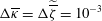 $\unicode[STIX]{x0394}\overline{\unicode[STIX]{x1D705}}=\unicode[STIX]{x0394}\widetilde{\overline{\unicode[STIX]{x1D701}}}=10^{-3}$
was chosen, but values up to
 $O(10^{-1})$
and higher give practically indistinguishable results. To obtain the needed functions
 $\widetilde{\unicode[STIX]{x1D6F9}}$
for each
 $\overline{\unicode[STIX]{x1D705}}_{w}$
, respectively for each
 $\widetilde{\overline{\unicode[STIX]{x1D701}}}_{w}$
, (2.19) was solved by collocation with the BVP4C-function implemented in Matlab (see previous discussion of figure 2). In figure 7, the numerical solutions for the lowest
 $\unicode[STIX]{x1D701}$
potential are compared to those obtained within the Debye–Hückel approximation (‘DH’, thin dashed lines) and given by (2.37), indicating good agreement for the case of non-overlapping EDLs.
For channels without EDL overlap (
 $\overline{\unicode[STIX]{x1D705}}_{0}\gtrsim 5$
),
 $\unicode[STIX]{x2202}_{\widehat{\unicode[STIX]{x1D6E9}}}\unicode[STIX]{x1D6F9}/\overline{\unicode[STIX]{x1D701}}$
vanishes further away from the EDL, particularly along the channel centre plane (see plots 7
c,d). For any value of the
 $\unicode[STIX]{x1D701}$
potential, the maximum of
 $\unicode[STIX]{x2202}_{\widehat{\unicode[STIX]{x1D6E9}}}\unicode[STIX]{x1D6F9}/\overline{\unicode[STIX]{x1D701}}$
occurs along the channel centre plane if
 $\overline{\unicode[STIX]{x1D705}}_{0}=1$
, while for the larger
 $\overline{\unicode[STIX]{x1D705}}_{0}$
values considered, it occurs at
 $Z\gtrsim 0.8$
. Along the channel wall,
 $\unicode[STIX]{x2202}_{\widehat{\unicode[STIX]{x1D6E9}}}\unicode[STIX]{x1D6F9}/\overline{\unicode[STIX]{x1D701}}$
is zero for all cases due to the given
 $\unicode[STIX]{x1D701}$
potential. Hence, the thermal modification of the EDL potential described by (2.33), respectively by (2.37), indeed leads to an axial electric field, which is restricted to the EDL only.
Local change of EDL potential with temperature expressed by
 $\unicode[STIX]{x2202}_{\widehat{\unicode[STIX]{x1D6E9}}}\unicode[STIX]{x1D6F9}(Z)/\overline{\unicode[STIX]{x1D701}}\equiv \unicode[STIX]{x2202}_{\widehat{\unicode[STIX]{x1D6E9}}}\unicode[STIX]{x1D713}(Z)/\unicode[STIX]{x1D701}$
for
 $\unicode[STIX]{x1D701}=[-25,-75,-125]\times 10^{-3}~\text{V}$
. In all plots, thermophoretic ion motion is considered with equal intrinsic Soret coefficients for each ion species (Soret A,
 $S_{0}=5\times 10^{-3}~\text{K}^{-1}$
). A temperature-dependent ion mobility and a temperature dependent dielectric permittivity is included (
 $M_{0}=-5.1\times 10^{-3}~\text{K}^{-1}$
) as well. The temperature difference equals
 $\unicode[STIX]{x0394}T=25~\text{K}$
, while the local temperature used for evaluation is
 $T=T_{0}+\unicode[STIX]{x0394}T$
. Numerical solutions (‘NM’, bold lines with symbols) were computed by means of (2.33) and compared for the lowest
 $\unicode[STIX]{x1D701}$
potential with those obtained within the Debye–Hückel approximation (‘DH’, thin dashed lines) and given by (2.37). In the plots (a–d), the nominal Debye parameter is varied according to
 $\overline{\unicode[STIX]{x1D705}}_{0}=\unicode[STIX]{x1D705}_{0}h=[1,5,10,50]$
. The legend shown in (a) is valid for (b–d) as well.

Appendix C. Verification of propulsion by the EDL potential
In the main text it is shown that under the sole presence of a thermal gradient a thermoosmotic velocity emerges in the channel, which under confinement contributes to the thermoelectric potential, even if the thermodiffusive mobilities of the ion species are identical (Soret A). Essentially, this is caused by an axial gradient of the EDL potential which propels the fluid by means of the electrohydrostatic pressure and the electrostatic body force (Maxwell stress). For an isothermal electrokinetic system, it is well known that the EDL itself does not set the fluid into motion. It was shown by Levich (Reference Levich1962, p. 484), that, for such systems, the electric body force due to the EDL and the osmotic pressure contribution exactly cancel each other and that only the externally applied electric field is relevant for the fluid propulsion (Pascall & Squires Reference Pascall and Squires2011). Therefore, the phenomenon described in this work may be suspected to be an artefact of the lubrication approximation (LA) used in the analysis. In the following, without relying on the LA, it is shown that a non-isothermal EDL can indeed propel the fluid (while an isothermal EDL cannot).
According to Fitts (Reference Fitts1962, p. 43), the incompressible Newtonian Navier–Stokes equation can be written as
 $$\begin{eqnarray}\displaystyle \unicode[STIX]{x1D70C}d_{t}\boldsymbol{v}-\unicode[STIX]{x1D702}\unicode[STIX]{x1D6FB}^{2}\boldsymbol{v}=-\unicode[STIX]{x1D735}p+\unicode[STIX]{x1D70C}_{0}\boldsymbol{Y}, & & \displaystyle\end{eqnarray}$$
where
 $\boldsymbol{Y}$
denotes the sum of all body forces. The right-hand side of (C 1) can be expressed by the general form of the Gibbs–Duhem equation for a multicomponent system (Fitts Reference Fitts1962, p. 44)
 $$\begin{eqnarray}\displaystyle \unicode[STIX]{x1D735}p-\unicode[STIX]{x1D70C}\boldsymbol{Y}=\mathop{\sum }_{k=1}^{P}\unicode[STIX]{x1D70C}_{k}\unicode[STIX]{x1D6FB}^{(T)}\unicode[STIX]{x1D707}_{k}^{\prime }. & & \displaystyle\end{eqnarray}$$
The mass of component
 $k$
per total volume
 $V$
is denoted by
 $\unicode[STIX]{x1D70C}_{k}$
. The sum contains all components
 $P=K+1$
, where
 $K$
is the number of solutes. The spatial gradient at constant temperature of the overall chemical potential is defined according to
 $$\begin{eqnarray}\displaystyle \unicode[STIX]{x1D6FB}^{(T)}\unicode[STIX]{x1D707}_{k}^{\prime }=\unicode[STIX]{x1D735}\unicode[STIX]{x1D707}_{k}^{\prime }-\unicode[STIX]{x2202}_{T}(\unicode[STIX]{x1D707}_{k})_{|p}\unicode[STIX]{x1D735}T, & & \displaystyle\end{eqnarray}$$
where
 $\unicode[STIX]{x1D707}_{k}=\unicode[STIX]{x1D707}_{k}^{\prime }-\unicode[STIX]{x1D708}_{k}F/M_{k}\unicode[STIX]{x1D719}$
(
 $M_{k}$
is the molar mass,
 $F=eN_{A}$
is the Faraday constant with
 $N_{A}$
as the Avogadro number). It is assumed that the gradient of the chemical potential of the solvent at constant temperature is negligibly small so that the effective upper limit of the sum in (C 2) is
 $K$
. No external potential is applied herein and
 $\unicode[STIX]{x1D719}\equiv \unicode[STIX]{x1D713}$
. The Nernst–Planck equations for the ion concentrations
 $n_{k}$
(
 $k=1,\ldots ,K$
) read
 $d_{t}n_{k}=-\unicode[STIX]{x1D735}\boldsymbol{\cdot }\boldsymbol{j}_{k}$
, where in agreement with (2.9) the diffusion flux density is given by
 $$\begin{eqnarray}\displaystyle \boldsymbol{j}_{k}=-D_{k}\unicode[STIX]{x1D735}n_{k}-n_{k}D_{T,k}\unicode[STIX]{x1D735}T-e\unicode[STIX]{x1D708}_{k}n_{k}\unicode[STIX]{x1D714}_{k}\unicode[STIX]{x1D735}\unicode[STIX]{x1D713}. & & \displaystyle\end{eqnarray}$$
In the latter equation,
 $D_{k}$
and
 $D_{T,k}$
are the Fickian and the thermal diffusion coefficients, respectively, of the ion species
 $k$
, while
 $\unicode[STIX]{x1D714}_{k}=D_{k}/(k_{B}T)$
are the electrophoretic mobilities. On the one hand, a vanishing flux density, indicating chemical equilibrium, is identical to
 $$\begin{eqnarray}\displaystyle e\unicode[STIX]{x1D708}_{k}\unicode[STIX]{x1D735}\unicode[STIX]{x1D713}+k_{B}T\unicode[STIX]{x1D735}[\ln (n_{k})+S_{k}T]=0, & & \displaystyle\end{eqnarray}$$
where
 $S_{k}=D_{T,k}/D_{k}$
. On the other hand, for a chemical potential
 $\unicode[STIX]{x1D707}_{k}^{\ast }=\unicode[STIX]{x1D707}_{k}^{\ast }(\unicode[STIX]{x1D713},n_{k},T)$
per number of ions, chemical equilibrium implies that
 $$\begin{eqnarray}\displaystyle \unicode[STIX]{x1D735}\unicode[STIX]{x1D707}_{k}^{\ast }=(\unicode[STIX]{x2202}_{\unicode[STIX]{x1D713}}\unicode[STIX]{x1D707}_{k}^{\ast })_{|n_{k},T}\unicode[STIX]{x1D735}\unicode[STIX]{x1D713}+(\unicode[STIX]{x2202}_{n_{k}}\unicode[STIX]{x1D707}_{k}^{\ast })_{|\unicode[STIX]{x1D713},T}\unicode[STIX]{x1D735}n_{k}+(\unicode[STIX]{x2202}_{T}\unicode[STIX]{x1D707}_{k}^{\ast })_{|\unicode[STIX]{x1D713},n_{k}}\unicode[STIX]{x1D735}T=0. & & \displaystyle\end{eqnarray}$$
Comparison with (C 5) defines the partial derivatives employed in (C 6) so that
 $\unicode[STIX]{x1D707}_{k}^{\ast }$
is defined according to
 $$\begin{eqnarray}\displaystyle \unicode[STIX]{x1D707}_{k}^{\ast }=e\unicode[STIX]{x1D708}_{k}\unicode[STIX]{x1D713}+k_{B}T[\ln (n_{k})+S_{k}T]. & & \displaystyle\end{eqnarray}$$
With the mass-specific chemical potential
 $\unicode[STIX]{x1D707}_{k}^{\prime }=N_{A}\unicode[STIX]{x1D707}_{k}^{\ast }/M_{k}$
and (C 3) one finds
 $$\begin{eqnarray}\displaystyle \unicode[STIX]{x1D6FB}^{(T)}\unicode[STIX]{x1D707}_{k}^{\prime }=\frac{\unicode[STIX]{x1D708}_{k}F}{M_{k}}\unicode[STIX]{x1D735}\unicode[STIX]{x1D713}+\frac{k_{B}TN_{A}}{M_{k}}\frac{\unicode[STIX]{x1D735}n_{k}}{n_{k}}. & & \displaystyle\end{eqnarray}$$
Employing
 $n_{k}=\unicode[STIX]{x1D70C}_{k}N_{A}/M_{k}$
and
 $\sum _{k=1}^{P}e\unicode[STIX]{x1D708}_{k}n_{k}=\sum _{k=1}^{K}e\unicode[STIX]{x1D708}_{k}n_{k}=\unicode[STIX]{x1D70C}_{f}$
(for the neutral solvent,
 $\unicode[STIX]{x1D708}_{P}=0$
) yields
 $$\begin{eqnarray}\displaystyle \mathop{\sum }_{k=1}^{K}\unicode[STIX]{x1D70C}_{k}\unicode[STIX]{x1D6FB}^{(T)}\unicode[STIX]{x1D707}_{k}^{\prime }=\unicode[STIX]{x1D70C}_{f}\unicode[STIX]{x1D735}\unicode[STIX]{x1D713}+k_{B}T\unicode[STIX]{x1D735}n, & & \displaystyle\end{eqnarray}$$
where
 $n=\sum _{k=1}^{K}n_{k}$
. The last term on the right-hand side is the gradient in osmotic pressure, i.e.
 $\unicode[STIX]{x1D735}p_{osm}=k_{B}T\unicode[STIX]{x1D735}n$
. At constant temperature, the right-hand side of (C 9) is identical to zero and the system is in mechanical equilibrium (Levich Reference Levich1962; Squires & Bazant Reference Squires and Bazant2004).
In the present non-isothermal case, for Soret A (
 $S_{-}=S_{+}=\overline{S}\approx S_{0}$
,
 $\unicode[STIX]{x0394}S=0$
), according to (2.18), the charge density can be replaced by
 $$\begin{eqnarray}\displaystyle \frac{\unicode[STIX]{x1D70C}_{f}}{e\unicode[STIX]{x1D708}n_{0}}=-2N\sinh (\widetilde{\unicode[STIX]{x1D6F9}}), & & \displaystyle\end{eqnarray}$$
while by summation of (2.17), one finds
 $$\begin{eqnarray}\displaystyle \frac{n}{n_{0}}=2N\cosh (\widetilde{\unicode[STIX]{x1D6F9}}). & & \displaystyle\end{eqnarray}$$
Hence, with the definitions
 $\unicode[STIX]{x1D6F9}=\unicode[STIX]{x1D713}e\unicode[STIX]{x1D708}/(k_{B}T_{0})$
and
 $\widetilde{\unicode[STIX]{x1D6F9}}=\unicode[STIX]{x1D6F9}/(1+\widehat{\unicode[STIX]{x1D6E9}})$
, one has
 $\unicode[STIX]{x1D735}\widetilde{\unicode[STIX]{x1D6F9}}=\unicode[STIX]{x1D735}\unicode[STIX]{x1D6F9}/(1+\widehat{\unicode[STIX]{x1D6E9}})-\widetilde{\unicode[STIX]{x1D6F9}}\unicode[STIX]{x1D735}\widehat{\unicode[STIX]{x1D6E9}}/(1+\widehat{\unicode[STIX]{x1D6E9}})$
. With this, (C 9) can be evaluated to read
 $$\begin{eqnarray}\displaystyle \mathop{\sum }_{k=1}^{K}\unicode[STIX]{x1D70C}_{k}\unicode[STIX]{x1D6FB}^{(T)}\unicode[STIX]{x1D707}_{k}^{\prime }=2k_{B}T_{0}n_{0}[(1+\widehat{\unicode[STIX]{x1D6E9}})\cosh (\widetilde{\unicode[STIX]{x1D6F9}})\unicode[STIX]{x1D735}N-N\widetilde{\unicode[STIX]{x1D6F9}}\sinh (\widetilde{\unicode[STIX]{x1D6F9}})\unicode[STIX]{x1D735}\widehat{\unicode[STIX]{x1D6E9}}]. & & \displaystyle\end{eqnarray}$$
In the present study,
 $N$
is a function of the local temperature
 $\widehat{\unicode[STIX]{x1D6E9}}=T/T_{0}$
so that both terms on the right-hand side of the latter equation differ from zero under non-isothermal conditions. This is also the case even if
 $N\equiv 1$
(no thermophoretic ion motion). The last term on the right-hand side of (C 12) is due to a temperature-dependent ion mobility, i.e. this effect alone leads to a thermoosmotic fluid propulsion in the EDL. Similarly, if
 $\unicode[STIX]{x1D735}\widehat{\unicode[STIX]{x1D6E9}}\equiv 0$
,
 $\unicode[STIX]{x1D735}N$
is not necessarily zero, e.g. if an axial gradient of the salt concentration is imposed. This resembles the classical case of solvent transport in osmotic capillaries. Finally, the system is in mechanical equilibrium only if
 $\unicode[STIX]{x1D735}N=\unicode[STIX]{x1D735}\widehat{\unicode[STIX]{x1D6E9}}=0$
.
The last term on the right-hand side of (C 12) vanishes outside the EDL where
 $\widetilde{\unicode[STIX]{x1D6F9}}\rightarrow 0$
. In the same limit,
 $\cosh (\widetilde{\unicode[STIX]{x1D6F9}})\rightarrow 1$
so that the right-hand side of (C 12) is equal to
 $\unicode[STIX]{x1D735}p_{drift}=2k_{B}Tn_{0}\unicode[STIX]{x1D735}N$
. This is the gradient in osmotic pressure of the ions due to the axial gradient in salt concentration (without interaction with the EDL). Herein it is assumed that this gradient is caused by the Soret thermodiffusion alone. This gradient is uniform across the channel and causes a constant drift of the ion cloud but no charge separation. Hence, the effective force density the ion cloud exerts on the solvent can be expressed by the sum of
 $\unicode[STIX]{x1D735}p_{drift}$
and the contribution due to the EDL. In linearized form, the latter reads
 $$\begin{eqnarray}\displaystyle -\boldsymbol{F}_{EDL} & = & \displaystyle \unicode[STIX]{x1D70C}_{f}\unicode[STIX]{x1D735}\unicode[STIX]{x1D713}+k_{B}T\unicode[STIX]{x1D735}n-\unicode[STIX]{x1D735}p_{drift}\nonumber\\ \displaystyle & {\approx} & \displaystyle 2k_{B}T_{0}n_{0}\{[\cosh (\unicode[STIX]{x1D6F9}^{(e)})-1]\unicode[STIX]{x1D735}N-\unicode[STIX]{x1D6F9}^{(e)}\sinh (\unicode[STIX]{x1D6F9}^{(e)})\unicode[STIX]{x1D735}\widehat{\unicode[STIX]{x1D6E9}}\},\end{eqnarray}$$
with
 $\unicode[STIX]{x1D6F9}^{(e)}$
being the EDL potential at isothermal conditions.
Thus, the mechanical propulsion observed in the non-isothermal case can be traced back to the circumstance that the divergence of the EDL Maxwell stress is not irrotational, while it appears to be under isothermal conditions. If a temperature-dependent ion mobility is included, the gradient of the osmotic pressure of the ion cloud itself is also not curl free while it is if only a thermophoretic ion motion is considered. In this context, in the present derivations discussed in the main text based on the LA and unlike in other studies of electrokinetics, an expression for the osmotic pressure of the ion cloud is never explicitly added to the governing equations as a body force. In the LA, a corresponding term automatically emerges from the momentum equation in the
 $z$
direction, (2.5). Its combination with the electromotive force in the EDL gives, under non-isothermal conditions, a non-vanishing force contribution. Note that within this derivation based on (C 2), the propulsion by a temperature-dependent dielectric permittivity is not captured. This is simply due to the Maxwell stress
 $-\unicode[STIX]{x1D70C}_{f}\unicode[STIX]{x1D735}\unicode[STIX]{x1D713}$
considered herein, which is not the full expression of the Korteweg–Helmholtz electric body force used in the main text.