1. Introduction
Owing to the crucial role of turbulence in industrial applications and its ubiquity in environmental processes, an enormous amount of research effort has been made in improving the current state of understanding and developing predictive models. In many practical systems, the turbulent flow is further complicated by the presence of a disperse phase (i.e. solid particles, liquid droplets or gaseous bubbles). Within the energy sector, disperse multiphase flows play fundamental roles in chemical transformation reactors (Basu & Fraser Reference Basu and Fraser1991; Bridgewater Reference Bridgewater1995; Marchisio & Fox Reference Marchisio and Fox2013), spray combustors (Lefebvre Reference Lefebvre1988; Lin & Reitz Reference Lin and Reitz1998) and slurry pipelines (Capecelatro & Desjardins Reference Capecelatro and Desjardins2013b ), to name just a few examples. Environmental processes, such as the growth of cloud droplets during rain formation (Shaw Reference Shaw2003; Grabowski & Wang Reference Grabowski and Wang2013), debris flows (Takahashi Reference Takahashi1981; Iverson, Reid & LaHusen Reference Iverson, Reid and LaHusen1997) and atmospheric dispersion of pollutant particles (Arya Reference Arya1999), are also of great interest within the scientific community. Improving our understanding of these flows is critical to developing strategies to control them and mitigate their negative effects. Meanwhile, the development of multiphase turbulence models severely lags their single-phase counterparts.
A key challenge in understanding and predicting disperse multiphase flows lies in the wide range of spatial and temporal scales that need to be considered. Important processes occurring at the scale of the particle (e.g. drag on the particle, inter-particle collisions, heat transfer and surface reactions) can cause the macroscopic behaviour to reach a variety of granular flow regimes, from dispersion and clustering in dilute particulate flows (Maxey Reference Maxey1987; Elghobashi & Truesdell Reference Elghobashi and Truesdell1992; Eaton & Fessler Reference Eaton and Fessler1994) to bubbling (Glasser, Sundaresan & Kevrekidis Reference Glasser, Sundaresan and Kevrekidis1998; Koch & Hill Reference Koch and Hill2001; Sundaresan Reference Sundaresan2003) and bed formation (Kennedy Reference Kennedy1963; Richards Reference Richards1980; Kidanemariam & Uhlmann Reference Kidanemariam and Uhlmann2014) in denser systems. Moreover, intimate coupling between the phases can often lead to a high degree of segregation from an initially homogeneous distribution of particles that reorganizes the underlying structure of the turbulent flow. In a recent experimental study, Shaffer et al. (Reference Shaffer, Gopalan, Breault, Cocco, Karri, Hays and Knowlton2013) observed high-speed jets of gas in risers of circulating fluidized bed reactors that were produced by particle clusters, a phenomenon referred to as jet bypassing. The interaction between clusters and the gas phase was shown to destroy the mixing behaviour of fluidized beds that makes them attractive for enhanced chemical reaction and heat transfer. Meanwhile, a fundamental understanding of particle clusters and their effect on the carrier phase remains elusive.
In an effort towards developing a macroscopic multiphase turbulence model, Fox (Reference Fox2014) recently derived the exact Reynolds-averaged (RA) equations for collisional fluid–particle flows. Through phase-space integration, the collisional Boltzmann equation was replaced by a set of macroscale moment equations. These equations were written in terms of particle-phase volume fraction
 ${\it\alpha}_{p}$
, particle-phase velocity
 $\boldsymbol{u}_{p}$
and granular temperature
 ${\it\Theta}$
, and were coupled to the carrier phase by including interactions through drag and buoyancy terms. Unlike in most previous derivations of turbulence models for moderately dense granular flows, a clear distinction was made between the granular temperature, which appears in the kinetic theory (KT) constitutive relations, and the particle-phase turbulent kinetic energy
 $k_{p}$
, which appears in the turbulent transport coefficients. The derivation by Fox (Reference Fox2014) is completely general and can be applied to any kinetic-based model for the disperse phase, including weakly and non-collisional flows, and leads to new insights about multiphase turbulence. For example, in addition to the classical production by mean shear, the transport equation for the fluid-phase turbulent kinetic energy
 $k_{f}$
contains an additional production term due to the mean velocity difference between the particle and fluid phases. In turn, this drag production mechanism gives rise to a separate class of multiphase turbulence, which we refer to as cluster-induced turbulence (CIT).
CIT occurs in fluid–particle flows when (i) the mean mass loading
 ${\it\varphi}$
, defined by the ratio of the specific masses of the particle and fluid phases, is of order one or larger and (ii) the difference between the mean phase velocities is non-zero. In statistically stationary flows, fluctuations in particle concentration can generate and sustain fluid-phase turbulence, which we refer to as fully developed CIT. In a recent paper, Zamansky et al. (Reference Zamansky, Coletti, Massot and Mani2014) show that a similar phenomenon occurs in the low-mass-loading regime when a particle-laden flow is subject to radiative heating. Because the material density ratio
 ${\it\rho}_{p}/{\it\rho}_{f}$
is very large in gas–particle flows, CIT is ubiquitous in practical engineering and environmental flows when body forces or inlet conditions generate a mean velocity difference, such as the gravity-driven flows studied herein. Surprisingly, despite its importance, very little is known about the fundamental properties of CIT, such as the mechanisms responsible for generating volume-fraction fluctuations, how energy is transferred between the phases, and how the cluster size distribution scales with various flow parameters.
In the literature, turbulent particle-laden flows are most often discussed in the dilute limit where the fluid-phase turbulence interacts with inertial particles without significant feedback from the particles (see e.g. Balachandar & Eaton Reference Balachandar and Eaton2010, and references therein). It is well established that dilute suspensions of heavy particles in isotropic turbulence will preferentially concentrate in regions of high strain rate and low vorticity (Eaton & Fessler Reference Eaton and Fessler1994). In the presence of gravity, numerical and experimental studies (e.g. Wang & Maxey Reference Wang and Maxey1993; Aliseda et al.
Reference Aliseda, Cartellier, Hainaux and Lasheras2002; Ferrante & Elghobashi Reference Ferrante and Elghobashi2003; Yang & Shy Reference Yang and Shy2003; Bosse, Kleiser & Meiburg Reference Bosse, Kleiser and Meiburg2006) have reported enhanced particle settling as a result of preferential sweeping, by which the particles tend towards regions of downward fluid motion when encountering vortical structures in the flow. In other words, the average fluid velocity seen by the particles is downwards. When two-way coupling between the phases is non-negligible, additional effects are responsible for enhancing the settling rate and spatial segregation of the particles. In local regions of high concentration, Bosse et al. (Reference Bosse, Kleiser and Meiburg2006) showed numerically that the particles exert a collective effect on the carrier phase, by which the fluid is accelerated due to particle drag. The enhanced downward fluid motion, in turn, leads to a larger particle settling velocity in these regions, which was reported to grow monotonically with increasing volume fraction. Ferrante & Elghobashi (Reference Ferrante and Elghobashi2003) showed that trajectory crossing of large particles through turbulent eddies creates local gradients in the fluid due to particle drag, causing the turbulence to become anisotropic, with a reduced decay rate of turbulence kinetic energy as compared to the unladen case. While the aforementioned studies may exhibit significant fluctuations in particle-phase velocity and number density in the dilute limit, in particular with
 ${\it\varphi}\ll 1$
, this particle-phase turbulence cannot exist in the absence of the fluid phase owing to the lack of momentum exchange between the particles. At higher values of mass loading, the relative motion between the phases leads to additional sources of instabilities as a result of interphase coupling (Glasser et al.
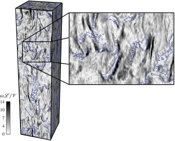
Reference Glasser, Sundaresan and Kevrekidis1998), giving rise to CIT. As depicted in figure 1, in gravity-driven CIT, particles accumulate in regions of low vorticity, as is seen in classical preferential concentration of low-mass-loading suspensions. However, in CIT the vorticity is generated in shear layers between clusters, unlike in classical preferential concentration, where vorticity would exist even in the absence of the disperse phase. In this high-mass-loading regime, the finite size of the particles cannot be ignored, leading to many numerical challenges.
Instantaneous field of fluid vorticity magnitude in gravity-driven CIT generated using data from Capecelatro, Desjardins & Fox (Reference Capecelatro, Desjardins and Fox2014a
) corresponding to
 $\mathit{Re}_{p}=1$
in this work (refer to table 1). Vorticity is generated by the shear layers at the edge of clusters, denoted by the blue lines showing iso-contours of
 ${\it\alpha}_{p}=3\langle {\it\alpha}_{p}\rangle$
.
With the advent of petascale computing in recent years, particle-resolved direct numerical simulations (PR-DNS) of three-dimensional gas–solid flows with
 $O(10^{4})$
particles have become feasible. A recent review article on PR-DNS development can be found in Tenneti & Subramaniam (Reference Tenneti and Subramaniam2014). Although its use is limited to relatively small ensembles of particles, too small to observe the macroscale turbulence that we wish to capture in this study, PR-DNS has provided new insights on the collective behaviour of fluid–particle flows that is useful for lower-cost simulation techniques. For example, Xu & Subramaniam (Reference Xu and Subramaniam2010) performed PR-DNS of a turbulent flow past uniform and clustered configurations of fixed particle assemblies using a discrete-time, direct-forcing, immersed-boundary method. The fluid-phase turbulence was found to be significantly anisotropic due to the fluid–particle interaction, and the level of turbulent kinetic energy in the fluid phase was always found to be greater in the clustered case compared to the uniform particle configuration. In another recent study, Shah et al. (Reference Shah, Utikar, Tade, Evans and Pareek2013) conducted lattice Boltzmann simulations of a single fixed cluster under a wide range of volume fractions and particle Reynolds numbers. The PR-DNS results revealed that particles arranged in a cluster configuration exhibited considerably lower drag than randomly arranged particles under the same flow conditions, with more significant reduction at lower particle Reynolds numbers.
Uhlmann & Doychev (Reference Uhlmann and Doychev2014) performed PR-DNS of gravity-induced settling particles in triply periodic domains in order to seek a critical Galileo number marking the onset of clustering. Although the study considered a dilute suspension of particles with a density ratio of 1.5, placing them outside the regime of CIT, particle clustering was still observed, and as a result the average particle settling velocity was reported to be increased by 12 % compared to the terminal velocity of an isolated sphere. The Galileo number,
 $\mathit{Ga}=u_{g}d_{p}/{\it\nu}_{f}$
, measures the ratio between gravitational and viscous forces acting on a submerged particle, where
 $d_{p}$
is the particle diameter,
 ${\it\nu}_{f}$
is the kinematic viscosity of the fluid and
 $u_{g}=(|{\it\rho}_{p}/{\it\rho}_{f}-1|d_{p}g)^{1/2}$
, with
 $g$
being the magnitude of the gravitational acceleration. It is interesting to note that, in gas–solid flows with
 ${\it\rho}_{p}\gg {\it\rho}_{f}$
,
 $u_{g}$
closely resembles the empirical model for the cluster fall velocity developed by Noymer & Glicksman (Reference Noymer and Glicksman2000). In their study, numerous experimental measurements of cluster fall velocities occurring in fluidized beds were compiled from the literature, observing that, although the flow conditions vary significantly, as well as the reactor geometries and particle parameters, the measured velocities were typically close to
 $1~\text{m}~\text{s}^{-1}$
, corresponding to
 $u_{cl}=0.75({\it\rho}_{p}/{\it\rho}_{f}d_{p}g)^{1/2}$
. In a recent numerical study, Capecelatro, Pepiot & Desjardins (Reference Capecelatro, Pepiot and Desjardins2014b
) demonstrated that clusters simulated in wall-bounded flows also fall with velocity
 $u_{cl}$
.
Owing to the excessive computational cost associated with PR-DNS, alternative approaches have been employed to study clustering in fluid–particle flows. Eulerian–Eulerian (EE) and Eulerian–Lagrangian (EL) methods have been used in numerous studies within the literature, with various levels of success. EE representations solve the gas phase and solid particles on a common Eulerian grid, greatly reducing the computational cost, as individual particles do not need to be tracked. In the limit where the flow is highly collisional and assumed to be nearly at equilibrium, the particle density function is close to Maxwellian and a Chapman–Enskog expansion can be used to derive a two-fluid model (TFM) using ensemble or volume averaging (Gidaspow Reference Gidaspow1994; Zhang & Prosperetti Reference Zhang and Prosperetti1994; Peirano & Leckner Reference Peirano and Leckner1998). Agrawal et al. (Reference Agrawal, Loezos, Syamlal and Sundaresan2001) employed TFM to simulate homogeneous gravity-driven CIT in both two- and three-dimensional domains. It was shown that global statistics were strongly dependent on the mesh size but became mesh-independent when the mesh size was of the order of a few particle diameters. It was further shown that clusters are not properly captured unless sufficient resolution is applied. In a more recent study, Ozel, Fede & Simonin (Reference Ozel, Fede and Simonin2013) studied the influence of unresolved structures (i.e. clusters) on drag force and particulate phase stresses in wall-bounded riser flows via TFM. It was shown that various subgrid terms have to be modelled in order to properly account for the presence of clusters.
EL strategies provide an alternative framework that typically relies on simpler closures compared to EE, where individual particle trajectories are solved using Newton’s laws of motion, and models are required for interphase exchange and particle collisions. Particle clustering in two-dimensional flows using the EL method can be found in a large number of studies (e.g. Tanaka et al. Reference Tanaka, Yonemura, Kiribayashi and Tsuji1996; Helland, Occelli & Tadrist Reference Helland, Occelli and Tadrist2002; Shuyan et al. Reference Shuyan, Huanpeng, Huilin, Wentie, Ding and Wei2005; He et al. Reference He, Deen, Annaland and Kuipers2009; Liu & Lu Reference Liu and Lu2009; Liu & Xu Reference Liu and Xu2009). In these studies, large-eddy simulation (LES) is often used to solve the gas-phase turbulence, and particle collisions are typically modelled stochastically by means of the direct simulation Monte Carlo (DSMC) method. Stochastic collision models are computationally more efficient in comparison to deterministic methods because information from neighbouring particles is not required. Instead, these methods rely on the generation of a fictitious collision partner with a given size and velocity (Sommerfeld Reference Sommerfeld2001). Because these models assume a behaviour for the particle and fluid-phase velocity fluctuations (e.g. Gaussian), accurate predictions of non-equilibrium flows are compromised. However, deterministic methods (Cundall & Strack Reference Cundall and Strack1979; Hoomans et al. Reference Hoomans, Kuipers, Briels and Van Swaaij1996) rely on the physical properties of each individual particle, and therefore non-trivial velocity distributions, such as trajectory crossings that are common in CIT, pose no additional challenges.
It has been demonstrated in recent work that two-dimensional simulations are only capable of capturing qualitative features of particle clustering in gravity-driven flows, while a fully three-dimensional description is required to accurately capture the quantitative behaviour (Capecelatro et al.
Reference Capecelatro, Pepiot and Desjardins2014b
; Li, Pannala & Shahnam Reference Li, Pannala and Shahnam2014). In particular, it was shown in our previous work that three-dimensional EL simulations are capable of accurately reproducing key cluster characteristics, including fall velocity, mean cluster concentration and concentration fluctuations in wall-bounded gravity-driven flows (Capecelatro et al.
Reference Capecelatro, Pepiot and Desjardins2014b
). The present paper is an extension of our previous work (Capecelatro et al.
Reference Capecelatro, Desjardins and Fox2014a
), in which EL simulations of fully developed gravity-driven CIT were performed. Starting from a random distribution of particles subject to gravity, after an initial transient, the flow becomes statistically stationary with a probability density function (p.d.f.) of particle-phase volume fraction that closely resembles a lognormal distribution. It was demonstrated that fully developed CIT exists with even the simplest possible phase coupling, i.e. Stokes drag with a characteristic time scale
 ${\it\tau}_{p}={\it\rho}_{p}d_{p}^{2}/(18{\it\rho}_{f}{\it\nu}_{f})$
, provided that the simulation domain is many times larger than the characteristic integral length scale defined by
 $\mathscr{L}={\it\tau}_{p}^{2}g$
. It was shown that a domain of size
 $64\mathscr{L}\times 16\mathscr{L}\times 16\mathscr{L}$
was required to obtain a fully developed flow unaffected by the periodic boundaries. Radl & Sundaresan (Reference Radl and Sundaresan2014) recently analysed homogeneous gravity-driven CIT in order to develop a drag model for filtered EL simulations that includes the effects of clusters. They conducted EL simulations under flow conditions similar to those of Capecelatro et al. (Reference Capecelatro, Desjardins and Fox2014a
) in a triply periodic box of size
 $5.85\mathscr{L}\times 1.46\mathscr{L}\times 1.46\mathscr{L}$
. It was found that a typical fluid grid resolution of
 $1.67d_{p}{-}3.33d_{p}$
is required to obtain grid-independent simulation results. They showed that a correction to the classical drag law must be included to account for unresolved clusters when conducting parcel-based simulations, in which only a subset of the particles are tracked. Owing to the size of their domain, however, it is likely that their reported results strongly depend on the periodic box size used in their simulations. For example, if the domain size is too small for falling clusters to avoid their own wake, it is likely that they will grow to the size of the domain and exhibit unrealistic settling velocities. As shown in Capecelatro et al. (Reference Capecelatro, Desjardins and Fox2014a
), the minimum domain size needed to avoid such numerical artifacts can be determined by examining two-point statistics such as the velocity correlation functions.
In an effort towards developing a predictive macroscopic turbulence model for fluid–particle flows, the primary goal of this study is to explore the physical mechanisms responsible for energy exchange between the phases in fully developed CIT and evaluate the unclosed terms that appear in the exact RA equations. To this end, we extend the analysis of Capecelatro et al. (Reference Capecelatro, Desjardins and Fox2014a
) to a range of particle Reynolds numbers, defined as
 $\mathit{Re}_{p}={\it\tau}_{p}gd_{p}/{\it\nu}_{f}$
. In addition, the RA formulation of Fox (Reference Fox2014) is further developed to include transport equations for the volume-fraction variance, the drift velocity and the separate components of the Reynolds stresses of each phase and particle pressure tensor. In the context of homogeneous CIT, the physics governing the one-point statistics involves a relatively small number of unclosed terms. For example, both the modification of the mean velocity difference due to clusters and the production of
 $k_{f}$
depend on a single term representing the difference between the fluid-phase-averaged fluid velocity
 $\langle \boldsymbol{u}_{f}\rangle _{f}=\langle {\it\alpha}_{f}\boldsymbol{u}_{f}\rangle /\langle {\it\alpha}_{f}\rangle$
, with
 ${\it\alpha}_{f}=1-{\it\alpha}_{p}$
being the fluid-phase volume fraction, and the particle-phase-averaged fluid velocity
 $\langle \boldsymbol{u}_{f}\rangle _{p}=\langle {\it\alpha}_{p}\boldsymbol{u}_{f}\rangle /\langle {\it\alpha}_{p}\rangle$
. In the literature on particle-laden flows,
 $\langle \boldsymbol{u}_{f}\rangle _{f}$
is sometimes referred to as the fluid-phase velocity seen by the fluid, and
 $\langle \boldsymbol{u}_{f}\rangle _{p}$
as the fluid-phase velocity seen by the particles. Because particle clusters arise spontaneously in CIT and are negatively correlated with the fluid velocity (see e.g. Capecelatro et al.
Reference Capecelatro, Desjardins and Fox2014a
), these two fluid velocities are not equal. To obtain accurate closures for the RA framework, fully developed gravity-driven CIT is simulated using the EL method, where the unsteady fluid motion is sufficiently captured by the mesh and the two phases are coupled through resolved contributions of the fluid stresses and a drag term. Inelastic particle collisions are handled deterministically via the soft-sphere approach originally proposed by Cundall & Strack (Reference Cundall and Strack1979). In this study we focus on fixed values of the mean particle-phase volume fraction
 $\langle {\it\alpha}_{p}\rangle =0.01$
and fluid–particle density ratio
 ${\it\rho}_{p}/{\it\rho}_{f}=1000$
, corresponding to a fixed mass loading of
 ${\it\varphi}=10.1$
, while three values of the particle Reynolds number are investigated, namely
 $\mathit{Re}_{p}=0.25$
, 0.5 and 1. The adaptive spatial filter introduced in our previous work (Capecelatro et al.
Reference Capecelatro, Desjardins and Fox2014a
) is used to decouple the instantaneous particle-phase turbulent kinetic energy
 $k_{p}$
from the granular temperature
 ${\it\Theta}$
. The filter enables the Lagrangian data to be evaluated as Eulerian fields that are consistent with the terms appearing in the RA equations. Key mechanisms responsible for energy exchange between the phases are quantified and discussed.
2. Multiscale description of collisional fluid–particle flows
The multiscale nature of particle-laden flows is impossible to ignore when developing a predictive multiphase turbulence model. This section presents mesoscale and macroscale equations describing the motion of monodisperse, collisional, solid particles suspended in an incompressible fluid. We begin by defining the various phase-average (PA) terms that must be considered in the multiscale description of particle-laden turbulence. A mesoscale model is then provided for the fluid–particle flow, where the particles are described in a Lagrangian frame and the fluid equations are derived from volume filtering the Navier–Stokes equations. A macroscopic Eulerian description of the particle phase is then presented, which, along with the fluid-phase equations, is the starting point for deriving the multiphase turbulence description given at the end of this section.
2.1. Spatial decomposition of the particle velocity field
In the context of high-inertia particles with response times that are long compared to the characteristic time scale of the turbulence, individual particle trajectories will retain information from previous collisions and interactions with distant turbulent eddies, causing them to deviate from fluid pathlines (Maxey Reference Maxey1987). Velocities of neighbouring particles may therefore be uncorrelated, while ensembles of particles collectively respond to large-scale motions of the flow. The instantaneous velocity of any particle
 $i$
,
 $\boldsymbol{v}_{p}^{(i)}$
, can be decomposed into a spatially correlated contribution
 $\boldsymbol{u}_{p}$
and an uncorrelated (residual) component
 ${\bf\delta}\boldsymbol{v}_{p}^{(i)}$
(Février, Simonin & Squires Reference Février, Simonin and Squires2005), i.e.
 $$\begin{eqnarray}\boldsymbol{v}_{p}^{(i)}(t)=\boldsymbol{u}_{p}[\boldsymbol{x}_{p}^{(i)}(t),t]+{\bf\delta}\boldsymbol{v}_{p}^{(i)}(t),\end{eqnarray}$$
where
 $\boldsymbol{x}_{p}^{(i)}$
is the centre position of particle
 $i$
. For a single realization of the flow, the total particle-phase fluctuating energy is given by
 $$\begin{eqnarray}{\it\kappa}_{p}={\textstyle \frac{1}{2}}\langle \boldsymbol{v}_{p}^{\prime }\boldsymbol{\cdot }\boldsymbol{v}_{p}^{\prime }\rangle ,\end{eqnarray}$$
where
 $\boldsymbol{v}_{p}^{\prime }=\boldsymbol{v}_{p}-\langle \boldsymbol{v}_{p}\rangle$
is the total fluctuation in particle velocity with the property
 $\langle \boldsymbol{v}_{p}^{\prime }\rangle =0$
. Note that the averaging operator
 $\langle (\cdot )\rangle$
is used throughout this work to denote a particle average when applied to a Lagrangian quantity, and a volume average when applied to an Eulerian quantity. Owing to the statistical stationarity and homogeneity of the flows considered in this work,
 $\langle (\cdot )\rangle$
is a function neither of the spatial coordinate
 $\boldsymbol{x}$
nor of time
 $t$
at steady state.
Analogous to Favre averaging in variable-density flows, the PA with respect to the particle phase, denoted by
 $\langle (\cdot )\rangle _{p}=\langle {\it\alpha}_{p}(\cdot )\rangle /\langle {\it\alpha}_{p}\rangle$
, is useful in multiphase modelling (Fox Reference Fox2014). Note that PA Eulerian quantities are identical to particle-average Lagrangian quantities, e.g.
 $\langle \boldsymbol{u}_{p}\rangle _{p}=\langle \boldsymbol{v}_{p}\rangle$
. Fluctuations about the PA velocity are expressed as
 $\boldsymbol{u}_{p}^{\prime \prime }(\boldsymbol{x},t)=\boldsymbol{u}_{p}(\boldsymbol{x},t)-\langle \boldsymbol{u}_{p}\rangle _{p}$
, with
 $\langle \boldsymbol{u}_{p}^{\prime \prime }\rangle _{p}=0$
. Using this definition, the PA particle-phase turbulent kinetic energy is defined as
 $$\begin{eqnarray}k_{p}={\textstyle \frac{1}{2}}\langle \boldsymbol{u}_{p}^{\prime \prime }\boldsymbol{\cdot }\boldsymbol{u}_{p}^{\prime \prime }\rangle _{p}.\end{eqnarray}$$
It is important to note that
 $\boldsymbol{u}_{p}^{\prime \prime }\neq \boldsymbol{u}_{p}^{\prime }$
, and therefore
 $\langle \boldsymbol{u}_{p}^{\prime \prime }\rangle \neq 0$
in general.
A quantitative measure of the local uncorrelated particle agitation is given by the granular temperature
 ${\it\Theta}$
, which is defined using the residual component of the instantaneous particle velocity
 ${\bf\delta}\boldsymbol{v}_{p}^{(i)}$
, such that the PA granular temperature is given by
 $$\begin{eqnarray}\langle {\it\Theta}\rangle _{p}={\textstyle \frac{1}{3}}\langle {\bf\delta}\boldsymbol{v}_{p}\boldsymbol{\cdot }{\bf\delta}\boldsymbol{v}_{p}\rangle .\end{eqnarray}$$
With these definitions, the total particle-phase fluctuation energy
 ${\it\kappa}_{p}$
corresponds to the sum of the correlated and uncorrelated granular energy, i.e.
 $$\begin{eqnarray}{\it\kappa}_{p}=k_{p}+{\textstyle \frac{3}{2}}\langle {\it\Theta}\rangle _{p}.\end{eqnarray}$$
The distinction between
 $k_{p}$
and
 $\langle {\it\Theta}\rangle _{p}$
is crucial in turbulence modelling. For instance, in the context of moderately dense particulate flows,
 $\langle {\it\Theta}\rangle _{p}$
is needed to evaluate the particle-phase viscosity and pressure, which arise due to collisions. Thus, failure to separate these two contributions will lead to a gross overprediction of the collision rate (Fox Reference Fox2014). Moreover, previous works (Hrenya & Sinclair Reference Hrenya and Sinclair1997; Février et al.
Reference Février, Simonin and Squires2005) have shown that the dissipation of
 $k_{p}$
enters as a source term for
 $\langle {\it\Theta}\rangle _{p}$
. This is analogous to single-phase flow, where dissipation of turbulent kinetic energy leads to viscous heating.
2.2. Mesoscale description of fluid–particle systems
A complete description of each particle and the interstitial fluid phase is provided by the microscale model, which solves the Navier–Stokes equation for the fluid with no-slip boundary conditions applied at the surface of each particle, along with Newton’s equations for the momentum of each individual particle (see e.g. Tenneti & Subramaniam Reference Tenneti and Subramaniam2014). However, its use is limited to relatively small ensembles of particles, typically too small to observe the macroscale turbulence that we wish to capture in this study. Consequently, a mesoscale model can be formulated from the microscopic description by introducing a set of variables that adequately describes the physics of the disperse phase (Subramaniam Reference Subramaniam2000; Fox Reference Fox2007). For systems containing a large number of particles, it is often convenient to define a number-density function
 $f(t,\boldsymbol{x},\boldsymbol{v}_{p})$
, which depends on time
 $t$
, position
 $\boldsymbol{x}$
and particle velocity
 $\boldsymbol{v}_{p}$
. The stochastic nature of the particle phase can be described by a kinetic equation given by
 $$\begin{eqnarray}\frac{\partial f}{\partial t}+\frac{\partial }{\partial \boldsymbol{x}}\boldsymbol{\cdot }(\boldsymbol{v}_{p}f)+\frac{\partial }{\partial \boldsymbol{v}_{p}}\boldsymbol{\cdot }[(\mathbf{\mathscr{A}}_{p}+\boldsymbol{g})f]=\mathbb{C},\end{eqnarray}$$
where
 $\mathbf{\mathscr{A}}_{p}$
is the acceleration due to fluid–particle interactions,
 $\boldsymbol{g}=[-g,0,0]^{\text{T}}$
is the acceleration due to gravity, and
 $\mathbb{C}$
is the collision operator. Owing to the large number of independent variables associated with
 $f$
in a three-dimensional flow, a direct solution of the kinetic equation is still expensive in most practical flows, and various mathematical approximations have been made to arrive at tractable mesoscale models. In a recent review paper, Fox (Reference Fox2012) summarizes such modelling strategies, in addition to providing a systematic approach for developing LES tools starting from microscale physics.
2.2.1. Lagrangian description of the particle phase
In Lagrangian methods, the disperse phase is solved by discretizing the distribution function
 $f$
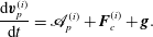
into a number of individually tracked notional particles. These notional particles (also referred to as parcels) are a statistical representation of the kinetic equation, and can produce accurate solutions given that a sufficient number of particles are used to control statistical noise (Bird Reference Bird1994). A single realization of the Lagrangian field accounts discretely for all individual particle processes, where the displacement of a particle
 $i$
is described by Newton’s second law of motion, i.e.
 $$\begin{eqnarray}\frac{\text{d}\boldsymbol{v}_{p}^{(i)}}{\text{d}t}=\mathbf{\mathscr{A}}_{p}^{(i)}+\boldsymbol{F}_{c}^{(i)}+\boldsymbol{g}.\end{eqnarray}$$
In this equation,
 $\boldsymbol{F}_{c}^{(i)}$
is the collision force experienced by particle
 $i$
, and the interphase exchange term is given by
 $$\begin{eqnarray}\mathbf{\mathscr{A}}_{p}^{(i)}=\frac{1}{{\it\tau}_{p}}(\boldsymbol{u}_{f}[\boldsymbol{x}_{p}^{(i)}]-\boldsymbol{v}_{p}^{(i)})-\frac{1}{{\it\rho}_{p}}\boldsymbol{{\rm\nabla}}p_{f}[\boldsymbol{x}_{p}^{(i)}]+\frac{1}{{\it\rho}_{p}}\boldsymbol{{\rm\nabla}}\boldsymbol{\cdot }{\bf\sigma}_{f}[\boldsymbol{x}_{p}^{(i)}],\end{eqnarray}$$
where the instantaneous fluid-phase velocity field
 $\boldsymbol{u}_{f}$
, pressure gradient
 $\boldsymbol{{\rm\nabla}}p_{f}$
and divergence of the viscous stress tensor
 $\boldsymbol{{\rm\nabla}}\boldsymbol{\cdot }{\bf\sigma}_{f}$
are evaluated at
 $\boldsymbol{x}_{p}^{(i)}$
, the centre position of particle
 $i$
. The exact definitions of the fluid-phase quantities will be made explicit below. In this work, it is assumed that
 ${\it\rho}_{p}\gg {\it\rho}_{f}$
, and therefore all other contributions from the fluid phase (e.g. added mass and lift forces) are neglected. Note that, with sufficient resolution of the fluid phase, the fluid stresses that appear in the interphase exchange (2.8) partially capture these additional effects. Also note that, in real systems with moderate Reynolds numbers and particle volume fractions, particles will experience drag with a nonlinear dependence on these terms (e.g. Beetstra, Van der Hoef & Kuipers Reference Beetstra, Van der Hoef and Kuipers2007; Tenneti, Garg & Subramaniam Reference Tenneti, Garg and Subramaniam2011), but, for consistency with the Reynolds-average formulation considered in this study, these higher-order terms are neglected.
2.2.2. Fluid-phase description
In order to account for the presence of particles in the fluid phase without requiring to resolve the boundary layers around individual particles, the microscale equations need to be modified. Anderson & Jackson (Reference Anderson and Jackson1967) derived a set of equations by applying a volume filtering operator to the Navier–Stokes equations, thereby replacing the microscale variables (fluid velocity, pressure, etc.) by smoother, locally filtered fields. This filtering approach introduces a separation in length scales, where everything smaller than the support of the filtering kernel requires modelling, and everything larger than the support of the filtering kernel is captured explicitly. Note that this idea of volume filtering will be revisited in later sections to develop a consistent methodology for extracting turbulence statistics. The volume-filtered conservation equations for a constant-density fluid are given by
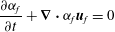 $$\begin{eqnarray}\frac{\partial {\it\alpha}_{f}}{\partial t}+\boldsymbol{{\rm\nabla}}\boldsymbol{\cdot }{\it\alpha}_{f}\boldsymbol{u}_{f}=0\end{eqnarray}$$
and
 $$\begin{eqnarray}\frac{\partial {\it\alpha}_{f}\boldsymbol{u}_{f}}{\partial t}+\boldsymbol{{\rm\nabla}}\boldsymbol{\cdot }{\it\alpha}_{f}\boldsymbol{u}_{f}\otimes \boldsymbol{u}_{f}=-\frac{1}{{\it\rho}_{f}}\boldsymbol{{\rm\nabla}}p_{f}+\frac{1}{{\it\rho}_{f}}\boldsymbol{{\rm\nabla}}\boldsymbol{\cdot }{\bf\sigma}_{f}-{\it\alpha}_{f}{\it\phi}\mathbf{\mathscr{A}}+{\it\alpha}_{f}\boldsymbol{g},\end{eqnarray}$$
where the mass loading is defined as
 $$\begin{eqnarray}{\it\phi}=\frac{{\it\rho}_{p}{\it\alpha}_{p}}{{\it\rho}_{f}{\it\alpha}_{f}}.\end{eqnarray}$$
Volume filtering the microscopic fluid stress tensor leads to unclosed terms, which can be modelled as an effective viscosity
 ${\it\nu}_{f}^{\star }$
that is added to the molecular viscosity
 ${\it\nu}_{f}$
. These unclosed stresses represent the enhanced dissipation due to unresolved fluid velocity fluctuations generated at the particle scale. Several theoretical and semi-empirical correlations for the effective viscosity exist in the literature (e.g. Einstein Reference Einstein1906; Thomas Reference Thomas1965; Gibilaro et al.
Reference Gibilaro, Gallucci, Di Felice and Pagliai2007). These expressions typically depend on local values of the particle-phase volume fraction, the particle Reynolds number and the mass loading. The fluid-phase viscous stress tensor is thus defined as
 $$\begin{eqnarray}{\bf\sigma}_{f}={\it\rho}_{f}({\it\nu}_{f}+{\it\nu}_{f}^{\star })[\boldsymbol{{\rm\nabla}}\boldsymbol{u}_{f}+(\boldsymbol{{\rm\nabla}}\boldsymbol{u}_{f})^{\text{T}}-{\textstyle \frac{2}{3}}\boldsymbol{{\rm\nabla}}\boldsymbol{\cdot }\boldsymbol{u}_{f}\unicode[STIX]{x1D644}],\end{eqnarray}$$
where
 $\unicode[STIX]{x1D644}$
is the identity tensor. Note that
 ${\it\nu}_{f}^{\star }$
is found to remain small compared to
 ${\it\nu}_{f}$
in this work, suggesting that this closure does not influence flow physics noticeably.
The interphase momentum exchange term that appears in (2.10) is given by
 $$\begin{eqnarray}\mathbf{\mathscr{A}}=\frac{1}{{\it\tau}_{p}}(\boldsymbol{u}_{f}-\boldsymbol{u}_{p})-\frac{1}{{\it\rho}_{p}}\boldsymbol{{\rm\nabla}}p_{f}+\frac{1}{{\it\rho}_{p}}\boldsymbol{{\rm\nabla}}\boldsymbol{\cdot }{\bf\sigma}_{f},\end{eqnarray}$$
where
 $\boldsymbol{u}_{p}$
is the instantaneous particle velocity (in the same frame as the fluid). Details on the formulation can be found in Capecelatro & Desjardins (Reference Capecelatro and Desjardins2013a
). Note that the contributions of the resolved stresses in (2.13) can be combined with the fluid stresses on the right-hand side of (2.10). However, these terms should be handled separately in numerical solutions in order to ensure conservation of momentum in the two phases. It should also be noted that volume filtering the microscopic fluid momentum equation will lead to a residual stress containing subfilter velocity fluctuations that requires closure, but is neglected in this work since the majority of the velocity fluctuations are assumed to be generated by clusters with typical length scales that are sufficiently resolved by the computational mesh. To confirm this assumption, an eddy viscosity model based on a Smagorinsky closure is tested and found to predict an eddy viscosity that remains smaller than 3 % of
 ${\it\nu}_{f}$
.
Starting from (2.10) and enforcing (2.9), a transport equation for the fluid-phase velocity tensor product is given by
 $$\begin{eqnarray}\displaystyle & & \displaystyle \frac{\partial {\it\alpha}_{f}\boldsymbol{u}_{f}\otimes \boldsymbol{u}_{f}}{\partial t}+\boldsymbol{{\rm\nabla}}\boldsymbol{\cdot }{\it\alpha}_{f}\boldsymbol{u}_{f}\otimes \boldsymbol{u}_{f}\otimes \boldsymbol{u}_{f}\nonumber\\ \displaystyle & & \displaystyle \quad =-\frac{1}{{\it\rho}_{f}}(\boldsymbol{u}_{f}\otimes \boldsymbol{{\rm\nabla}}p_{f})^{\dagger }+\frac{1}{{\it\rho}_{f}}(\boldsymbol{u}_{f}\otimes \boldsymbol{{\rm\nabla}}\boldsymbol{\cdot }{\bf\sigma}_{f})^{\dagger }-{\it\alpha}_{f}{\it\phi}(\boldsymbol{u}_{f}\otimes \mathbf{\mathscr{A}})^{\dagger }+{\it\alpha}_{f}(\boldsymbol{u}_{f}\otimes \boldsymbol{g})^{\dagger }.\qquad\end{eqnarray}$$
Hereinafter, to simplify the notation, the sum of any second-order tensor
 $(\cdot )$
with its transpose is denoted by
 $(\cdot )^{\dagger }=(\cdot )+(\cdot )^{\text{T}}$
.
2.3. Eulerian description of the particle phase
The Eulerian description of the particle phase is formulated in terms of moments of the mesoscopic kinetic model (2.6). The governing equations take the form of Eulerian transport equations with coupling terms between the phases due to mass and momentum exchange. The KT model of granular flows (Jenkins & Savage Reference Jenkins and Savage1983) is now generally accepted as a valid macroscale description of moderately dense particle flows. In this regime, the particle volume fraction is large enough such that particle–particle collisions drive the velocity distribution function towards the equilibrium (Maxwellian) distribution, though not too large that particles remain in sustained contact. Assuming that the particles are frictionless hard spheres of equal density and diameter (i.e. monodisperse) and that collisions are nearly elastic, the conservation of mass and momentum in the presence of a constant-density fluid are given by
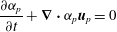 $$\begin{eqnarray}\frac{\partial {\it\alpha}_{p}}{\partial t}+\boldsymbol{{\rm\nabla}}\boldsymbol{\cdot }{\it\alpha}_{p}\boldsymbol{u}_{p}=0\end{eqnarray}$$
and
 $$\begin{eqnarray}\frac{\partial {\it\alpha}_{p}\boldsymbol{u}_{p}}{\partial t}+\boldsymbol{{\rm\nabla}}\boldsymbol{\cdot }{\it\alpha}_{p}(\boldsymbol{u}_{p}\otimes \boldsymbol{u}_{p}+\unicode[STIX]{x1D64B})={\it\alpha}_{p}(\mathbf{\mathscr{A}}+\boldsymbol{g}).\end{eqnarray}$$
From (2.16), the transport equation for the particle-phase velocity tensor product can be obtained as
 $$\begin{eqnarray}\frac{\partial {\it\alpha}_{p}\boldsymbol{u}_{p}\otimes \boldsymbol{u}_{p}}{\partial t}+\boldsymbol{{\rm\nabla}}\boldsymbol{\cdot }({\it\alpha}_{p}\boldsymbol{u}_{p}\otimes \boldsymbol{u}_{p}\otimes \boldsymbol{u}_{p})+[\boldsymbol{u}_{p}\otimes \boldsymbol{{\rm\nabla}}\boldsymbol{\cdot }({\it\alpha}_{p}\unicode[STIX]{x1D64B})]^{\dagger }={\it\alpha}_{p}[\boldsymbol{u}_{p}\otimes (\mathbf{\mathscr{A}}+\boldsymbol{g})]^{\dagger }.\end{eqnarray}$$
It is typically assumed that the particle-phase Knudsen number is very small so that a Chapman–Enskog expansion can be used to provide constitutive relations for the pressure tensor
 $\unicode[STIX]{x1D64B}$
(Lun et al.
Reference Lun, Savage, Jeffrey and Chepuriny1984). However, for non-equilibrium flows, a transport equation for the pressure tensor is necessary. Defining the second-order moment of the velocity distribution function as
 $\unicode[STIX]{x1D614}^{2}=\int \boldsymbol{v}_{p}\otimes \boldsymbol{v}_{p}f\,\text{d}\boldsymbol{v}_{p}$
, from (2.6) and (2.17) the transport equation for the central moment
 ${\it\alpha}_{p}\unicode[STIX]{x1D64B}=\unicode[STIX]{x1D614}^{2}-{\it\alpha}_{p}\boldsymbol{u}_{p}\otimes \boldsymbol{u}_{p}$
can be derived:
 $$\begin{eqnarray}\frac{\partial {\it\alpha}_{p}\unicode[STIX]{x1D64B}}{\partial t}+\boldsymbol{{\rm\nabla}}\boldsymbol{\cdot }{\it\alpha}_{p}(\boldsymbol{u}_{p}\otimes \unicode[STIX]{x1D64B}+\unicode[STIX]{x1D64C})=-{\it\alpha}_{p}(\unicode[STIX]{x1D64B}\boldsymbol{\cdot }\boldsymbol{{\rm\nabla}}\boldsymbol{u}_{p})^{\dagger }-\frac{2}{{\it\tau}_{p}}{\it\alpha}_{p}\unicode[STIX]{x1D64B}+\frac{12}{\sqrt{{\rm\pi}}d_{p}}{\it\alpha}_{p}^{2}{\it\Theta}^{1/2}({\it\Delta}^{\star }-\unicode[STIX]{x1D64B}).\end{eqnarray}$$
In this equation,
 $\unicode[STIX]{x1D64C}$
is a heat-flux tensor that contains the third-order central moments of the velocity distribution function, and the last term on the right-hand side is the particle–particle collision term that has been closed using the Bhatnagar–Gross–Krook (BGK) approximation (Bhatnagar, Gross & Krook Reference Bhatnagar, Gross and Krook1954) extended to inelastic collisions (Passalacqua et al.
Reference Passalacqua, Galvin, Vedula, Hrenya and Fox2011), where
 ${\it\Theta}=\text{tr}(\unicode[STIX]{x1D64B})/3$
is the granular temperature,
 $0\leqslant e\leqslant 1$
is the coefficient of restitution and
 ${\it\Delta}^{\star }$
is the second-order moment of the collisional equilibrium distribution, given by
 $$\begin{eqnarray}{\it\Delta}^{\star }={\textstyle \frac{1}{4}}(1+e)^{2}{\it\Theta}\unicode[STIX]{x1D644}+{\textstyle \frac{1}{4}}(1-e)^{2}\unicode[STIX]{x1D64B}.\end{eqnarray}$$
In the limit of elastic collisions (
 $e=1$
), the collision term on the right-hand side of (2.18) contains only contributions from the deviatoric pressure tensor.
The particle-phase pressure tensor can be decomposed into an isotropic contribution
 ${\it\Theta}\unicode[STIX]{x1D644}$
and the particle-phase viscous stress tensor defined by
 ${\bf\sigma}_{p}={\it\Theta}\unicode[STIX]{x1D644}-\unicode[STIX]{x1D64B}$
. By taking one-third of the trace of (2.18), the equation for the granular temperature is found to be
 $$\begin{eqnarray}\frac{\partial {\it\alpha}_{p}{\it\Theta}}{\partial t}+\boldsymbol{{\rm\nabla}}\boldsymbol{\cdot }{\it\alpha}_{p}\left(\boldsymbol{u}_{p}{\it\Theta}+\frac{2}{3}\boldsymbol{q}\right)=-\frac{2}{3}{\it\alpha}_{p}\unicode[STIX]{x1D64B}\boldsymbol{ : }\boldsymbol{{\rm\nabla}}\boldsymbol{u}_{p}-\frac{2}{{\it\tau}_{p}}{\it\alpha}_{p}{\it\Theta}-\frac{6(1-e^{2})}{\sqrt{{\rm\pi}}d_{p}}{\it\alpha}_{p}^{2}{\it\Theta}^{3/2},\end{eqnarray}$$
where
 $\boldsymbol{q}$
is the granular energy flux. The second term on the right-hand side of (2.20) represents the loss of granular energy due to drag, and the last term is dissipation due to inelastic collisions. The first term on the right-hand side of (2.20) can be rewritten using the decomposition
 $\unicode[STIX]{x1D64B}\boldsymbol{ : }\boldsymbol{{\rm\nabla}}\boldsymbol{u}_{p}={\it\Theta}\boldsymbol{{\rm\nabla}}\boldsymbol{\cdot }\boldsymbol{u}_{p}-{\bf\sigma}_{p}\boldsymbol{ : }\boldsymbol{{\rm\nabla}}\boldsymbol{u}_{p}$
. The contribution
 $-{\it\alpha}_{p}{\it\Theta}\boldsymbol{{\rm\nabla}}\boldsymbol{\cdot }\boldsymbol{u}_{p}$
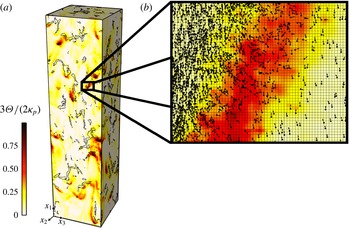
represents compressive heating of the particle phase, while the second contribution represents production due to viscous dissipation of mean kinetic energy. As shown in figure 2, taken from Capecelatro et al. (Reference Capecelatro, Desjardins and Fox2014a
), compressive heating upstream of falling clusters makes an important contribution to the granular temperature balance in CIT.
Instantaneous field of granular temperature generated using data from Capecelatro et al. (Reference Capecelatro, Desjardins and Fox2014a
) corresponding to
 $\mathit{Re}_{p}=1$
in this work (refer to table 1). Full domain showing iso-contours of
 ${\it\alpha}_{p}=3\langle {\it\alpha}_{p}\rangle$
(a) and zoomed-in snapshot showing particle velocity vectors in the vicinity of a cluster (b). High values of the granular temperature correspond to regions in front of falling clusters where the particle-phase velocity
 $\boldsymbol{u}_{p}$
is strongly compressed in the vertical direction. Particle size and mesh are shown to scale.
2.4. Reynolds-average equations of motion
The wide range of length and time scales associated with turbulent multiphase flows makes a direct solution of the transport equations presented thus far intractable for many environmental and industrial applications. It is therefore necessary to obtain from first principles a set of macroscopic equations that can correctly capture the statistical properties of the flow. Here we present the exact RA transport equations recently derived by Fox (Reference Fox2014), and extend the analysis to include the full Reynolds stress and granular stress equations. The relevant unclosed terms that are retained in the context of homogeneous gravity-driven flows are then presented and discussed.
2.4.1. Reynolds-average particle-phase equations
Taking the RA of (2.15) yields
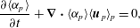 $$\begin{eqnarray}\frac{\partial \langle {\it\alpha}_{p}\rangle }{\partial t}+\boldsymbol{{\rm\nabla}}\boldsymbol{\cdot }\langle {\it\alpha}_{p}\rangle \langle \boldsymbol{u}_{p}\rangle _{p}=0,\end{eqnarray}$$
where
 $\langle {\it\alpha}_{p}\rangle$
is the RA particle volume fraction and
 $\langle \boldsymbol{u}_{p}\rangle _{p}=\langle {\it\alpha}_{p}\boldsymbol{u}_{p}\rangle /\langle {\it\alpha}_{p}\rangle$
is the PA particle-phase velocity. There are no unclosed terms in (2.21). Starting from (2.15), the transport equation for the variance of particle-phase volume fraction is found to be
 $$\begin{eqnarray}\displaystyle & & \displaystyle \frac{\partial \langle {\it\alpha}_{p}^{\prime 2}\rangle }{\partial t}+\boldsymbol{{\rm\nabla}}\boldsymbol{\cdot }\langle {\it\alpha}_{p}^{\prime 2}\rangle \langle \boldsymbol{u}_{p}\rangle _{p}+\boldsymbol{{\rm\nabla}}\boldsymbol{\cdot }\langle {\it\alpha}_{p}^{\prime 2}\boldsymbol{u}_{p}^{\prime \prime }\rangle \nonumber\\ \displaystyle & & \displaystyle \quad =-2\langle {\it\alpha}_{p}^{\prime }\boldsymbol{u}_{p}^{\prime \prime }\rangle \boldsymbol{\cdot }\boldsymbol{{\rm\nabla}}\langle {\it\alpha}_{p}\rangle -\langle {\it\alpha}_{p}^{\prime 2}\rangle \boldsymbol{{\rm\nabla}}\boldsymbol{\cdot }\langle \boldsymbol{u}_{p}\rangle _{p}-2\langle {\it\alpha}_{p}\rangle \langle {\it\alpha}_{p}^{\prime }\boldsymbol{{\rm\nabla}}\boldsymbol{\cdot }\boldsymbol{u}_{p}^{\prime \prime }\rangle -\langle {\it\alpha}_{p}^{\prime 2}\boldsymbol{{\rm\nabla}}\boldsymbol{\cdot }\boldsymbol{u}_{p}^{\prime \prime }\rangle ,\qquad\end{eqnarray}$$
where particle-phase velocity fluctuations are defined by
 $\boldsymbol{u}_{p}^{\prime \prime }=\boldsymbol{u}_{p}-\langle \boldsymbol{u}_{p}\rangle _{p}$
, and fluctuations about a RA quantity are denoted by a single prime. The second and third terms on the left-hand side of (2.22) represent transport due to the mean and fluctuating particle velocity. The first term on the right-hand side is the usual variance production term due to gradients in the mean volume fraction. The remaining terms represent production and/or dissipation of variance due to the particle-phase mean (
 $-\boldsymbol{{\rm\nabla}}\boldsymbol{\cdot }\langle \boldsymbol{u}_{p}\rangle _{p}$
) and fluctuating (
 $-\boldsymbol{{\rm\nabla}}\boldsymbol{\cdot }\boldsymbol{u}_{p}^{\prime \prime }$
) rate of compression.
Taking the RA of (2.16) yields
 $$\begin{eqnarray}\frac{\partial \langle {\it\alpha}_{p}\rangle \langle \boldsymbol{u}_{p}\rangle _{p}}{\partial t}+\boldsymbol{{\rm\nabla}}\boldsymbol{\cdot }\langle {\it\alpha}_{p}\rangle (\langle \boldsymbol{u}_{p}\rangle _{p}\otimes \langle \boldsymbol{u}_{p}\rangle _{p}+\langle \mathbf{\mathscr{P}}\rangle _{p})=\langle {\it\alpha}_{p}\rangle (\langle \mathbf{\mathscr{A}}\rangle _{p}+\boldsymbol{g}),\end{eqnarray}$$
where
 $\langle \mathbf{\mathscr{P}}\rangle _{p}=\langle \unicode[STIX]{x1D64B}\rangle _{p}+\langle \boldsymbol{u}_{p}^{\prime \prime }\otimes \boldsymbol{u}_{p}^{\prime \prime }\rangle _{p}$
is the sum of the particle stress tensor and the particle-phase Reynolds stress, and
 $$\begin{eqnarray}\langle \mathbf{\mathscr{A}}\rangle _{p}=\frac{1}{{\it\tau}_{p}}(\langle \boldsymbol{u}_{f}\rangle _{p}-\langle \boldsymbol{u}_{p}\rangle _{p})+\frac{1}{{\it\rho}_{p}}(\langle \boldsymbol{{\rm\nabla}}\boldsymbol{\cdot }{\bf\sigma}_{f}\rangle _{p}-\langle \boldsymbol{{\rm\nabla}}p_{f}\rangle _{p}).\end{eqnarray}$$
The fluid-phase variables that are averaged with respect to the particle phase, i.e.
 $\langle \boldsymbol{u}_{f}\rangle _{p}$
,
 $\langle \boldsymbol{{\rm\nabla}}\boldsymbol{\cdot }{\bf\sigma}_{f}\rangle _{p}$
and
 $\langle \boldsymbol{{\rm\nabla}}p_{f}\rangle _{p}$
, appear due to fluid–particle coupling and require closure. In the literature, these terms are sometimes referred to as the fluid-phase statistics seen by the particles (see appendix A for further discussion of this topic).
The PA particle stress tensor that appears in
 $\langle \mathbf{\mathscr{P}}\rangle _{p}$
is expressed as
 $$\begin{eqnarray}\displaystyle & & \displaystyle \frac{\partial \langle {\it\alpha}_{p}\rangle \langle \unicode[STIX]{x1D64B}\rangle _{p}}{\partial t}+\boldsymbol{{\rm\nabla}}\boldsymbol{\cdot }\langle {\it\alpha}_{p}\rangle (\langle \boldsymbol{u}_{p}\rangle _{p}\otimes \langle \unicode[STIX]{x1D64B}\rangle _{p}+\langle \boldsymbol{u}_{p}^{\prime \prime }\otimes \unicode[STIX]{x1D64B}\rangle _{p}+\langle \unicode[STIX]{x1D64C}\rangle _{p})\nonumber\\ \displaystyle & & \displaystyle \quad =-\langle {\it\alpha}_{p}\rangle (\langle \unicode[STIX]{x1D64B}\rangle _{p}\boldsymbol{\cdot }\boldsymbol{{\rm\nabla}}\langle \boldsymbol{u}_{p}\rangle _{p}+\langle \unicode[STIX]{x1D64B}\boldsymbol{\cdot }\boldsymbol{{\rm\nabla}}\boldsymbol{u}_{p}^{\prime \prime }\rangle _{p})^{\dagger }-\frac{2}{{\it\tau}_{p}}\langle {\it\alpha}_{p}\rangle \langle \unicode[STIX]{x1D64B}\rangle _{p}+\frac{12\langle {\it\alpha}_{p}\rangle }{\sqrt{{\rm\pi}}d_{p}}\langle {\it\alpha}_{p}{\it\Theta}^{1/2}({\it\Delta}^{\star }-\unicode[STIX]{x1D64B})\rangle _{p},\nonumber\\ \displaystyle & & \displaystyle\end{eqnarray}$$
where the PA heat flux
 $\langle \unicode[STIX]{x1D64C}\rangle _{p}$
and collision terms are unclosed and require further evaluation. Taking the RA of the granular temperature transport equation (2.20) (or one-third of the trace of (2.25)) yields
 $$\begin{eqnarray}\displaystyle & & \displaystyle \frac{\partial \langle {\it\alpha}_{p}\rangle \langle {\it\Theta}\rangle _{p}}{\partial t}+\boldsymbol{{\rm\nabla}}\boldsymbol{\cdot }\langle {\it\alpha}_{p}\rangle \left(\langle \boldsymbol{u}_{p}\rangle _{p}\langle {\it\Theta}\rangle _{p}+\langle \boldsymbol{u}_{p}^{\prime \prime }{\it\Theta}\rangle _{p}+\frac{2}{3}\langle \boldsymbol{q}\rangle _{p}\right)\nonumber\\ \displaystyle & & \displaystyle \quad =-\frac{2}{3}\langle {\it\alpha}_{p}\rangle (\langle \unicode[STIX]{x1D64B}\rangle _{p}\boldsymbol{ : }\boldsymbol{{\rm\nabla}}\langle \boldsymbol{u}_{p}\rangle _{p}+\langle \unicode[STIX]{x1D64B}\boldsymbol{ : }\boldsymbol{{\rm\nabla}}\boldsymbol{u}_{p}^{\prime \prime }\rangle _{p})-\frac{2}{{\it\tau}_{p}}\langle {\it\alpha}_{p}\rangle \langle {\it\Theta}\rangle _{p}-\frac{6(1-e^{2})}{\sqrt{{\rm\pi}}d_{p}}\langle {\it\alpha}_{p}^{2}{\it\Theta}^{3/2}\rangle .\qquad \quad\end{eqnarray}$$
In this equation, the turbulent granular temperature flux
 $\langle \boldsymbol{u}_{p}^{\prime \prime }{\it\Theta}\rangle _{p}$
, the production term
 $\langle {\it\alpha}_{p}\rangle \langle \unicode[STIX]{x1D64B}\boldsymbol{ : }\boldsymbol{{\rm\nabla}}\boldsymbol{u}_{p}^{\prime \prime }\rangle _{p}$
and the collisional dissipation term
 $\langle {\it\alpha}_{p}^{2}{\it\Theta}^{3/2}\rangle$
are unclosed and require further evaluation. The contribution due to the correlation between the particle stress tensor and velocity gradients can be further decomposed as
 $\langle \unicode[STIX]{x1D64B}\boldsymbol{ : }\boldsymbol{{\rm\nabla}}\boldsymbol{u}_{p}^{\prime \prime }\rangle _{p}=\langle {\it\Theta}\boldsymbol{{\rm\nabla}}\boldsymbol{\cdot }\boldsymbol{u}_{p}^{\prime \prime }\rangle _{p}-\langle {\bf\sigma}_{p}\boldsymbol{ : }\boldsymbol{{\rm\nabla}}\boldsymbol{u}_{p}^{\prime \prime }\rangle _{p}$
, i.e. turbulent compressive heating and turbulent viscous dissipation, respectively.
Starting from the PA particle-phase velocity in (2.23), a transport equation for the particle-phase mean velocity tensor product is given by
 $$\begin{eqnarray}\displaystyle & & \displaystyle \frac{\partial \langle {\it\alpha}_{p}\rangle \langle \boldsymbol{u}_{p}\rangle _{p}\otimes \langle \boldsymbol{u}_{p}\rangle _{p}}{\partial t}+\boldsymbol{{\rm\nabla}}\boldsymbol{\cdot }\langle {\it\alpha}_{p}\rangle [\langle \boldsymbol{u}_{p}\rangle _{p}\otimes \langle \boldsymbol{u}_{p}\rangle _{p}\otimes \langle \boldsymbol{u}_{p}\rangle _{p}+(\langle \mathbf{\mathscr{P}}\rangle _{p}\otimes \langle \boldsymbol{u}_{p}\rangle _{p})^{\dagger }]\nonumber\\ \displaystyle & & \displaystyle \quad =\langle {\it\alpha}_{p}\rangle [\langle \mathbf{\mathscr{P}}\rangle _{p}\boldsymbol{\cdot }\boldsymbol{{\rm\nabla}}\langle \boldsymbol{u}_{p}\rangle _{p}+\langle \boldsymbol{u}_{p}\rangle _{p}\otimes (\langle \mathbf{\mathscr{A}}\rangle _{p}+\boldsymbol{g})]^{\dagger }.\end{eqnarray}$$
The first term on the right-hand side of (2.27) represents contributions to kinetic energy transfer from both the Reynolds stress tensor and mean granular temperature. Taking half the trace of (2.27) yields
 $$\begin{eqnarray}\displaystyle & & \displaystyle \frac{\partial \langle {\it\alpha}_{p}\rangle K_{p}}{\partial t}+\boldsymbol{{\rm\nabla}}\boldsymbol{\cdot }\langle {\it\alpha}_{p}\rangle (\langle \boldsymbol{u}_{p}\rangle _{p}K_{p}+\langle \mathbf{\mathscr{P}}\rangle _{p}\boldsymbol{\cdot }\langle \boldsymbol{u}_{p}\rangle _{p})\nonumber\\ \displaystyle & & \displaystyle \quad =\langle {\it\alpha}_{p}\rangle [\langle \mathbf{\mathscr{P}}\rangle _{p}\boldsymbol{ : }\boldsymbol{{\rm\nabla}}\langle \boldsymbol{u}_{p}\rangle _{p}+\langle \boldsymbol{u}_{p}\rangle _{p}\boldsymbol{\cdot }(\langle \mathbf{\mathscr{A}}\rangle _{p}+\boldsymbol{g})],\end{eqnarray}$$
where the particle-phase mean kinetic energy is defined as
 $$\begin{eqnarray}K_{p}={\textstyle \frac{1}{2}}\langle \boldsymbol{u}_{p}\rangle _{p}\boldsymbol{\cdot }\langle \boldsymbol{u}_{p}\rangle _{p}.\end{eqnarray}$$
The transport equation for the particle-phase Reynolds stress tensor is computed by subtracting (2.27) from the RA of (2.17), yielding
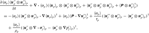 $$\begin{eqnarray}\displaystyle & & \displaystyle \frac{\partial \langle {\it\alpha}_{p}\rangle \langle \boldsymbol{u}_{p}^{\prime \prime }\otimes \boldsymbol{u}_{p}^{\prime \prime }\rangle _{p}}{\partial t}+\boldsymbol{{\rm\nabla}}\boldsymbol{\cdot }\langle {\it\alpha}_{p}\rangle (\langle \boldsymbol{u}_{p}\rangle _{p}\otimes \langle \boldsymbol{u}_{p}^{\prime \prime }\otimes \boldsymbol{u}_{p}^{\prime \prime }\rangle _{p}+\langle \boldsymbol{u}_{p}^{\prime \prime }\otimes \boldsymbol{u}_{p}^{\prime \prime }\otimes \boldsymbol{u}_{p}^{\prime \prime }\rangle _{p}+\langle \unicode[STIX]{x1D64B}\otimes \boldsymbol{u}_{p}^{\prime \prime }\rangle _{p}^{\dagger })\nonumber\\ \displaystyle & & \displaystyle \quad =-\langle {\it\alpha}_{p}\rangle (\langle \boldsymbol{u}_{p}^{\prime \prime }\otimes \boldsymbol{u}_{p}^{\prime \prime }\rangle _{p}\boldsymbol{\cdot }\boldsymbol{{\rm\nabla}}\langle \boldsymbol{u}_{p}\rangle _{p})^{\dagger }+\langle {\it\alpha}_{p}\rangle \langle \unicode[STIX]{x1D64B}\boldsymbol{\cdot }\boldsymbol{{\rm\nabla}}\boldsymbol{u}_{p}^{\prime \prime }\rangle _{p}^{\dagger }+\frac{\langle {\it\alpha}_{p}\rangle }{{\it\tau}_{p}}(\langle \boldsymbol{u}_{f}^{\prime \prime \prime }\otimes \boldsymbol{u}_{p}^{\prime \prime }\rangle _{p}-\langle \boldsymbol{u}_{p}^{\prime \prime }\otimes \boldsymbol{u}_{p}^{\prime \prime }\rangle _{p})^{\dagger }\nonumber\\ \displaystyle & & \displaystyle \qquad +\,\frac{\langle {\it\alpha}_{p}\rangle }{{\it\rho}_{p}}(\langle \boldsymbol{u}_{p}^{\prime \prime }\otimes \boldsymbol{{\rm\nabla}}\boldsymbol{\cdot }{\bf\sigma}_{f}^{\prime }\rangle _{p}-\langle \boldsymbol{u}_{p}^{\prime \prime }\otimes \boldsymbol{{\rm\nabla}}p_{f}^{\prime }\rangle _{p})^{\dagger },\end{eqnarray}$$
where the fluid-phase velocity fluctuations are defined as
 $\boldsymbol{u}_{f}^{\prime \prime \prime }=\boldsymbol{u}_{f}-\langle \boldsymbol{u}_{f}\rangle _{f}$
, with the PA fluid-phase velocity given by
 $\langle \boldsymbol{u}_{f}\rangle _{f}=\langle {\it\alpha}_{f}\boldsymbol{u}_{f}\rangle /\langle {\it\alpha}_{f}\rangle$
. The first term on the right-hand side of this equation is a second-order tensor that represents production due to the particle-phase Reynolds stresses and the particle-phase mean velocity gradients. The second term on the right-hand side represents redistribution and dissipation of the Reynolds stresses. Note that the same term appears in (2.25), but with the opposite sign. The third term on the right-hand side denotes energy exchange between the phases via drag. If we take half the trace of (2.30), the transport equation for the particle-phase turbulent kinetic energy is given by
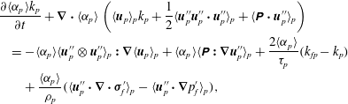 $$\begin{eqnarray}\displaystyle & & \displaystyle \frac{\partial \langle {\it\alpha}_{p}\rangle k_{p}}{\partial t}+\boldsymbol{{\rm\nabla}}\boldsymbol{\cdot }\langle {\it\alpha}_{p}\rangle \left(\langle \boldsymbol{u}_{p}\rangle _{p}k_{p}+\frac{1}{2}\langle \boldsymbol{u}_{p}^{\prime \prime }\boldsymbol{u}_{p}^{\prime \prime }\boldsymbol{\cdot }\boldsymbol{u}_{p}^{\prime \prime }\rangle _{p}+\langle \unicode[STIX]{x1D64B}\boldsymbol{\cdot }\boldsymbol{u}_{p}^{\prime \prime }\rangle _{p}\right)\nonumber\\ \displaystyle & & \displaystyle \quad =-\langle {\it\alpha}_{p}\rangle \langle \boldsymbol{u}_{p}^{\prime \prime }\otimes \boldsymbol{u}_{p}^{\prime \prime }\rangle _{p}\boldsymbol{ : }\boldsymbol{{\rm\nabla}}\langle \boldsymbol{u}_{p}\rangle _{p}+\langle {\it\alpha}_{p}\rangle \langle \unicode[STIX]{x1D64B}\boldsymbol{ : }\boldsymbol{{\rm\nabla}}\boldsymbol{u}_{p}^{\prime \prime }\rangle _{p}+\frac{2\langle {\it\alpha}_{p}\rangle }{{\it\tau}_{p}}(k_{fp}-k_{p})\nonumber\\ \displaystyle & & \displaystyle \qquad +\,\frac{\langle {\it\alpha}_{p}\rangle }{{\it\rho}_{p}}(\langle \boldsymbol{u}_{p}^{\prime \prime }\boldsymbol{\cdot }\boldsymbol{{\rm\nabla}}\boldsymbol{\cdot }{\bf\sigma}_{f}^{\prime }\rangle _{p}-\langle \boldsymbol{u}_{p}^{\prime \prime }\boldsymbol{\cdot }\boldsymbol{{\rm\nabla}}p_{f}^{\prime }\rangle _{p}),\end{eqnarray}$$
where
 $k_{fp}=\langle \boldsymbol{u}_{f}^{\prime \prime \prime }\boldsymbol{\cdot }\boldsymbol{u}_{p}^{\prime \prime }\rangle _{p}/2$
is the fluid–particle velocity cross-correlation. It should be noted that the turbulent dissipation of
 $k_{p}$
in (2.31),
 $\langle \unicode[STIX]{x1D64B}\boldsymbol{ : }\boldsymbol{{\rm\nabla}}\boldsymbol{u}_{p}^{\prime \prime }\rangle _{p}$
, appears as a source term for
 $\langle {\it\Theta}\rangle _{p}$
in (2.26), analogous to single-phase flow where dissipation of turbulent kinetic energy leads to viscous heating. In this case, however, dissipation is directly attributed to anisotropy in the particle stress tensor, i.e. to
 ${\bf\sigma}_{p}$
.
2.4.2. Reynolds-average fluid-phase equations
Taking the RA of (2.9) yields the transport equation for the RA fluid-phase volume fraction:
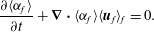 $$\begin{eqnarray}\frac{\partial \langle {\it\alpha}_{f}\rangle }{\partial t}+\boldsymbol{{\rm\nabla}}\boldsymbol{\cdot }\langle {\it\alpha}_{f}\rangle \langle \boldsymbol{u}_{f}\rangle _{f}=0.\end{eqnarray}$$
There are no unclosed terms in (2.32). The PA fluid-phase velocity equation found from (2.10) is given by
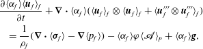 $$\begin{eqnarray}\displaystyle & & \displaystyle \frac{\partial \langle {\it\alpha}_{f}\rangle \langle \boldsymbol{u}_{f}\rangle _{f}}{\partial t}+\boldsymbol{{\rm\nabla}}\boldsymbol{\cdot }\langle {\it\alpha}_{f}\rangle (\langle \boldsymbol{u}_{f}\rangle _{f}\otimes \langle \boldsymbol{u}_{f}\rangle _{f}+\langle \boldsymbol{u}_{f}^{\prime \prime \prime }\otimes \boldsymbol{u}_{f}^{\prime \prime \prime }\rangle _{f})\nonumber\\ \displaystyle & & \displaystyle \quad =\frac{1}{{\it\rho}_{f}}(\boldsymbol{{\rm\nabla}}\boldsymbol{\cdot }\langle {\bf\sigma}_{f}\rangle -\boldsymbol{{\rm\nabla}}\langle p_{f}\rangle )-\langle {\it\alpha}_{f}\rangle {\it\varphi}\langle \mathbf{\mathscr{A}}\rangle _{p}+\langle {\it\alpha}_{f}\rangle \boldsymbol{g},\end{eqnarray}$$
where
 $$\begin{eqnarray}{\it\varphi}=\frac{{\it\rho}_{p}\langle {\it\alpha}_{p}\rangle }{{\it\rho}_{f}\langle {\it\alpha}_{f}\rangle }\end{eqnarray}$$
is the mean mass loading. The new unclosed terms that appear in (2.33) include the fluid-phase Reynolds stress tensor
 $\langle \boldsymbol{u}_{f}^{\prime \prime \prime }\otimes \boldsymbol{u}_{f}^{\prime \prime \prime }\rangle _{f}$
and the RA fluid-phase viscous stress tensor
 $\langle {\bf\sigma}_{f}\rangle$
.
The transport equation for the fluid-phase Reynolds stress tensor is given by
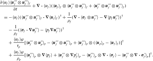 $$\begin{eqnarray}\displaystyle & & \displaystyle \frac{\partial \langle {\it\alpha}_{f}\rangle \langle \boldsymbol{u}_{f}^{\prime \prime \prime }\otimes \boldsymbol{u}_{f}^{\prime \prime \prime }\rangle _{f}}{\partial t}+\boldsymbol{{\rm\nabla}}\boldsymbol{\cdot }\langle {\it\alpha}_{f}\rangle (\langle \boldsymbol{u}_{f}\rangle _{f}\otimes \langle \boldsymbol{u}_{f}^{\prime \prime \prime }\otimes \boldsymbol{u}_{f}^{\prime \prime \prime }\rangle _{f}+\langle \boldsymbol{u}_{f}^{\prime \prime \prime }\otimes \boldsymbol{u}_{f}^{\prime \prime \prime }\otimes \boldsymbol{u}_{f}^{\prime \prime \prime }\rangle _{f})\nonumber\\ \displaystyle & & \displaystyle \quad =-\langle {\it\alpha}_{f}\rangle (\langle \boldsymbol{u}_{f}^{\prime \prime \prime }\otimes \boldsymbol{u}_{f}^{\prime \prime \prime }\rangle _{f}\boldsymbol{\cdot }\boldsymbol{{\rm\nabla}}\langle \boldsymbol{u}_{f}\rangle _{f})^{\dagger }+\frac{1}{{\it\rho}_{f}}(\boldsymbol{{\rm\nabla}}\boldsymbol{\cdot }\langle {\bf\sigma}_{f}\otimes \boldsymbol{u}_{f}^{\prime \prime \prime }\rangle -\boldsymbol{{\rm\nabla}}\langle p_{f}\boldsymbol{u}_{f}^{\prime \prime \prime }\rangle )^{\dagger }\nonumber\\ \displaystyle & & \displaystyle \qquad -\,\frac{1}{{\it\rho}_{f}}(\langle {\bf\sigma}_{f}\boldsymbol{\cdot }\boldsymbol{{\rm\nabla}}\boldsymbol{u}_{f}^{\prime \prime \prime }\rangle -\langle p_{f}\boldsymbol{{\rm\nabla}}\boldsymbol{u}_{f}^{\prime \prime \prime }\rangle )^{\dagger }\nonumber\\ \displaystyle & & \displaystyle \qquad +\,\frac{\langle {\it\alpha}_{f}\rangle {\it\varphi}}{{\it\tau}_{p}}[\langle \boldsymbol{u}_{f}^{\prime \prime \prime }\otimes \boldsymbol{u}_{p}^{\prime \prime }\rangle _{p}-\langle \boldsymbol{u}_{f}^{\prime \prime \prime }\otimes \boldsymbol{u}_{f}^{\prime \prime \prime }\rangle _{p}+\langle \boldsymbol{u}_{f}^{\prime \prime \prime }\rangle _{p}\otimes (\langle \boldsymbol{u}_{p}\rangle _{p}-\langle \boldsymbol{u}_{f}\rangle _{f})]^{\dagger }\nonumber\\ \displaystyle & & \displaystyle \qquad +\,\frac{\langle {\it\alpha}_{f}\rangle {\it\varphi}}{{\it\rho}_{p}}[\langle \boldsymbol{u}_{f}^{\prime \prime \prime }\rangle _{p}\otimes \boldsymbol{{\rm\nabla}}\langle p_{f}\rangle +\langle \boldsymbol{u}_{f}^{\prime \prime \prime }\otimes \boldsymbol{{\rm\nabla}}p_{f}^{\prime }\rangle _{p}-\langle \boldsymbol{u}_{f}^{\prime \prime \prime }\rangle _{p}\otimes \boldsymbol{{\rm\nabla}}\boldsymbol{\cdot }\langle {\bf\sigma}_{f}\rangle -\langle \boldsymbol{u}_{f}^{\prime \prime \prime }\otimes \boldsymbol{{\rm\nabla}}\boldsymbol{\cdot }{\bf\sigma}_{f}^{\prime }\rangle _{p}]^{\dagger }.\nonumber\\ \displaystyle & & \displaystyle\end{eqnarray}$$
The unclosed terms involving the fluid velocity fluctuations and fluid stresses are common to compressible flows. The terms involving a PA with respect to the particle phase represent turbulence generation mechanisms due to preferential segregation of particles and require closure. In the context of homogeneous gravity-driven gas–particle flows, mesoscale structures (i.e. particle clusters) generate volume-fraction and velocity fluctuations that can sustain the fluid turbulence even in the absence of mean shear (Capecelatro et al.
Reference Capecelatro, Desjardins and Fox2014a
). These flows are the focus of this work. In (2.35), the principal production term for the fluid-phase Reynolds stress tensor is
 $\langle \boldsymbol{u}_{f}^{\prime \prime \prime }\rangle _{p}\otimes (\langle \boldsymbol{u}_{p}\rangle _{p}-\langle \boldsymbol{u}_{f}\rangle _{f})$
, which we refer to as drag production.
The fluid-phase turbulent kinetic energy
 $k_{f}$
is defined as half the trace of (2.35), and is given by
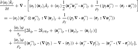 $$\begin{eqnarray}\displaystyle & & \displaystyle \frac{\partial \langle {\it\alpha}_{f}\rangle k_{f}}{\partial t}+\boldsymbol{{\rm\nabla}}\boldsymbol{\cdot }\left[\langle {\it\alpha}_{f}\rangle \langle \boldsymbol{u}_{f}\rangle _{f}k_{f}+\langle {\it\alpha}_{f}\rangle \frac{1}{2}\langle \boldsymbol{u}_{f}^{\prime \prime \prime }\boldsymbol{u}_{f}^{\prime \prime \prime }\boldsymbol{\cdot }\boldsymbol{u}_{f}^{\prime \prime \prime }\rangle _{f}+\frac{1}{{\it\rho}_{f}}(\langle p_{f}\boldsymbol{u}_{f}^{\prime \prime \prime }\rangle -\langle {\bf\sigma}_{f}\boldsymbol{\cdot }\boldsymbol{u}_{f}^{\prime \prime \prime }\rangle )\right]\nonumber\\ \displaystyle & & \displaystyle \quad =-\langle {\it\alpha}_{f}\rangle \langle \boldsymbol{u}_{f}^{\prime \prime \prime }\otimes \boldsymbol{u}_{f}^{\prime \prime \prime }\rangle _{f}\boldsymbol{ : }\boldsymbol{{\rm\nabla}}\langle \boldsymbol{u}_{f}\rangle _{f}+\frac{1}{{\it\rho}_{f}}(\langle p_{f}\boldsymbol{{\rm\nabla}}\boldsymbol{\cdot }\boldsymbol{u}_{f}^{\prime \prime \prime }\rangle -\langle {\bf\sigma}_{f}\boldsymbol{ : }\boldsymbol{{\rm\nabla}}\boldsymbol{u}_{f}^{\prime \prime \prime }\rangle )\nonumber\\ \displaystyle & & \displaystyle \qquad +\,\frac{\langle {\it\alpha}_{f}\rangle {\it\varphi}}{{\it\tau}_{p}}[2k_{fp}-2k_{f@p}+\langle \boldsymbol{u}_{f}^{\prime \prime \prime }\rangle _{p}\boldsymbol{\cdot }(\langle \boldsymbol{u}_{p}\rangle _{p}-\langle \boldsymbol{u}_{f}\rangle _{f})]\nonumber\\ \displaystyle & & \displaystyle \qquad +\,\frac{\langle {\it\alpha}_{f}\rangle {\it\varphi}}{{\it\rho}_{p}}[\langle \boldsymbol{u}_{f}^{\prime \prime \prime }\rangle _{p}\boldsymbol{\cdot }(\boldsymbol{{\rm\nabla}}\langle p_{f}\rangle -\boldsymbol{{\rm\nabla}}\boldsymbol{\cdot }\langle {\bf\sigma}_{f}\rangle )+\langle \boldsymbol{u}_{f}^{\prime \prime \prime }\boldsymbol{\cdot }\boldsymbol{{\rm\nabla}}p_{f}^{\prime }\rangle _{f}-\langle \boldsymbol{u}_{f}^{\prime \prime \prime }\boldsymbol{\cdot }(\boldsymbol{{\rm\nabla}}\boldsymbol{\cdot }{\bf\sigma}_{f}^{\prime })\rangle _{f}],\end{eqnarray}$$
where
 $k_{f@p}=\langle \boldsymbol{u}_{f}^{\prime \prime \prime }\boldsymbol{\cdot }\boldsymbol{u}_{f}^{\prime \prime \prime }\rangle _{p}/2$
is the fluid turbulent kinetic energy seen by the particles. As in single-phase turbulent flow,
 $\langle {\bf\sigma}_{f}\boldsymbol{ : }\boldsymbol{{\rm\nabla}}\boldsymbol{u}_{f}^{\prime \prime \prime }\rangle$
represents the turbulent kinetic energy dissipation rate. In (2.36), the principal production term for the fluid-phase turbulent kinetic energy is the drag production term
 $\langle \boldsymbol{u}_{f}^{\prime \prime \prime }\rangle _{p}\boldsymbol{\cdot }(\langle \boldsymbol{u}_{p}\rangle _{p}-\langle \boldsymbol{u}_{f}\rangle _{f})$
.
2.4.3. Application to homogeneous gravity-driven flow
In the context of fully developed homogeneous gravity-driven flow, the PA hydrodynamic variables are statistically invariant in space and the RA particle-phase equations reduce to
 $$\begin{eqnarray}\displaystyle & \displaystyle \frac{\partial \langle {\it\alpha}_{p}\rangle }{\partial t}=0, & \displaystyle\end{eqnarray}$$
 $$\begin{eqnarray}\displaystyle & \displaystyle \frac{\partial \langle {\it\alpha}_{p}^{\prime 2}\rangle }{\partial t}=-2\langle {\it\alpha}_{p}\rangle \langle {\it\alpha}_{p}^{\prime }\boldsymbol{{\rm\nabla}}\boldsymbol{\cdot }\boldsymbol{u}_{p}^{\prime \prime }\rangle -\langle {\it\alpha}_{p}^{\prime 2}\boldsymbol{{\rm\nabla}}\boldsymbol{\cdot }\boldsymbol{u}_{p}^{\prime \prime }\rangle , & \displaystyle\end{eqnarray}$$
 $$\begin{eqnarray}\displaystyle & \displaystyle \frac{\partial \langle \boldsymbol{u}_{p}\rangle _{p}}{\partial t}=\frac{1}{{\it\tau}_{p}}(\langle \boldsymbol{u}_{f}\rangle _{p}-\langle \boldsymbol{u}_{p}\rangle _{p})+\frac{1}{{\it\rho}_{p}}(\langle \boldsymbol{{\rm\nabla}}\boldsymbol{\cdot }{\bf\sigma}_{f}\rangle _{p}-\langle \boldsymbol{{\rm\nabla}}p_{f}\rangle _{p})+\boldsymbol{g}, & \displaystyle\end{eqnarray}$$
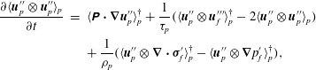 $$\begin{eqnarray}\displaystyle \frac{\partial \langle \boldsymbol{u}_{p}^{\prime \prime }\otimes \boldsymbol{u}_{p}^{\prime \prime }\rangle _{p}}{\partial t} & = & \displaystyle \langle \unicode[STIX]{x1D64B}\boldsymbol{\cdot }\boldsymbol{{\rm\nabla}}\boldsymbol{u}_{p}^{\prime \prime }\rangle _{p}^{\dagger }+\frac{1}{{\it\tau}_{p}}(\langle \boldsymbol{u}_{p}^{\prime \prime }\otimes \boldsymbol{u}_{f}^{\prime \prime \prime }\rangle _{p}^{\dagger }-2\langle \boldsymbol{u}_{p}^{\prime \prime }\otimes \boldsymbol{u}_{p}^{\prime \prime }\rangle _{p})\nonumber\\ \displaystyle & & \displaystyle +\,\frac{1}{{\it\rho}_{p}}(\langle \boldsymbol{u}_{p}^{\prime \prime }\otimes \boldsymbol{{\rm\nabla}}\boldsymbol{\cdot }{\bf\sigma}_{f}^{\prime }\rangle _{p}^{\dagger }-\langle \boldsymbol{u}_{p}^{\prime \prime }\otimes \boldsymbol{{\rm\nabla}}p_{f}^{\prime }\rangle _{p}^{\dagger }),\end{eqnarray}$$
 $$\begin{eqnarray}\frac{\partial \langle \unicode[STIX]{x1D64B}\rangle _{p}}{\partial t}=-\langle \unicode[STIX]{x1D64B}\boldsymbol{\cdot }\boldsymbol{{\rm\nabla}}\boldsymbol{u}_{p}^{\prime \prime }\rangle _{p}^{\dagger }-\frac{2}{{\it\tau}_{p}}\langle \unicode[STIX]{x1D64B}\rangle _{p}+\frac{12}{\sqrt{{\rm\pi}}d_{p}}\langle {\it\alpha}_{p}{\it\Theta}^{1/2}({\it\Delta}^{\star }-\unicode[STIX]{x1D64B})\rangle _{p}\end{eqnarray}$$
and
 $$\begin{eqnarray}\frac{\partial \langle {\it\Theta}\rangle _{p}}{\partial t}=-\frac{2}{3}\langle \unicode[STIX]{x1D64B}\boldsymbol{ : }\boldsymbol{{\rm\nabla}}\boldsymbol{u}_{p}^{\prime \prime }\rangle _{p}-\frac{2}{{\it\tau}_{p}}\langle {\it\Theta}\rangle _{p}-\frac{6(1-e^{2})}{\sqrt{{\rm\pi}}d_{p}}\langle {\it\alpha}_{p}{\it\Theta}^{3/2}\rangle _{p}.\end{eqnarray}$$
From (2.38), we see that
 $2\langle {\it\alpha}_{p}\rangle \langle {\it\alpha}_{p}^{\prime }\boldsymbol{{\rm\nabla}}\boldsymbol{\cdot }\boldsymbol{u}_{p}^{\prime \prime }\rangle +\langle {\it\alpha}_{p}^{\prime 2}\boldsymbol{{\rm\nabla}}\boldsymbol{\cdot }\boldsymbol{u}_{p}^{\prime \prime }\rangle =0$
at steady state. From (2.39), it is shown that the transport of the PA particle-phase velocity results in a balance between the forces exchanged by the fluid (i.e. drag model and resolved surface stresses) and gravity.
In a homogeneous flow with gravity directed in the negative
 $x_{1}$
direction, the only non-zero component of the PA particle-phase velocity is
 $\langle u_{p,1}\rangle _{p}$
:
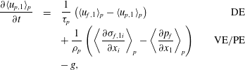 $$\begin{eqnarray}\displaystyle \begin{array}{@{}rclr@{}}\displaystyle \frac{\partial \langle u_{p,1}\rangle _{p}}{\partial t} & = & \displaystyle \frac{1}{{\it\tau}_{p}}\left(\langle u_{f,1}\rangle _{p}-\langle u_{p,1}\rangle _{p}\right) & \quad \text{DE}\\ & & +\,\displaystyle \frac{1}{{\it\rho}_{p}}\left(\left\langle \frac{\partial {\it\sigma}_{f,1i}}{\partial x_{i}}\right\rangle _{p}-\left\langle \frac{\partial p_{f}}{\partial x_{1}}\right\rangle _{p}\right) & \quad \text{VE}/\text{PE}\\ & & -\,g, & \end{array} & & \displaystyle \nonumber\\ \displaystyle & & \displaystyle\end{eqnarray}$$
where
 $x_{1}$
is the streamwise (gravity-aligned) component of the spatial coordinate
 $\boldsymbol{x}$
,
 $u_{p,1}$
and
 $u_{f,1}$
correspond to the streamwise components of the particle and fluid-phase velocities, respectively, and the subscript on the fluid-phase viscous stress tensor denotes its rank-1 components,
 ${\it\sigma}_{f,ij}$
represents the
 $(i,j)$
component of the stress tensor, and Einstein’s summation convention is used. The terms for viscous exchange (VE) and pressure exchange (PE) require further investigation, but are expected to be small for gas–particle flows where
 ${\it\rho}_{p}\gg {\it\rho}_{f}$
, and thus the particle-phase momentum involves a balance between the drag exchange (DE) term and gravity. Similar to the particle-phase velocity, the only non-zero component of the PA fluid-phase velocity seen by the particles in homogeneous gravity-driven flows is
 $\langle u_{f,1}\rangle _{p}$
, and at steady state we can observe that
 $\langle u_{f,1}\rangle _{p}\approx \langle u_{p,1}\rangle _{p}+{\it\tau}_{p}g$
.
Owing to homogeneity of the flow, the off-diagonal terms in (2.40) are null, and the transport equations for the normal components of the PA particle-phase Reynolds stress are given by
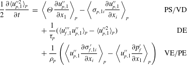 $$\begin{eqnarray}\displaystyle \begin{array}{@{}rclr@{}}\displaystyle \frac{1}{2}\frac{\partial \langle u_{p,1}^{\prime \prime 2}\rangle _{p}}{\partial t}\ & =\ & \displaystyle \left\langle {\it\Theta}\frac{\partial u_{p,1}^{\prime \prime }}{\partial x_{1}}\right\rangle _{p}-\left\langle {\it\sigma}_{p,1i}\frac{\partial u_{p,1}^{\prime \prime }}{\partial x_{i}}\right\rangle _{p} & \text{PS}/\text{VD}\\ \ & \ & +\,\displaystyle \frac{1}{{\it\tau}_{p}}(\langle u_{f,1}^{\prime \prime \prime }u_{p,1}^{\prime \prime }\rangle _{p}-\langle u_{p,1}^{\prime \prime 2}\rangle _{p}) & \text{DE}\\ \ & \ & +\,\displaystyle \frac{1}{{\it\rho}_{p}}\left(\left\langle u_{p,1}^{\prime \prime }\frac{\partial {\it\sigma}_{f,1i}^{\prime }}{\partial x_{i}}\right\rangle _{p}-\left\langle u_{p,1}^{\prime \prime }\frac{\partial p_{f}^{\prime }}{\partial x_{1}}\right\rangle _{p}\right) & \text{VE}/\text{PE}\end{array} & & \displaystyle \nonumber\\ \displaystyle & & \displaystyle\end{eqnarray}$$
and
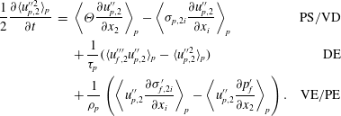 $$\begin{eqnarray}\displaystyle \begin{array}{@{}rclr@{}}\displaystyle \frac{1}{2}\frac{\partial \langle u_{p,2}^{\prime \prime 2}\rangle _{p}}{\partial t}\ & =\ & \displaystyle \left\langle {\it\Theta}\frac{\partial u_{p,2}^{\prime \prime }}{\partial x_{2}}\right\rangle _{p}-\left\langle {\it\sigma}_{p,2i}\frac{\partial u_{p,2}^{\prime \prime }}{\partial x_{i}}\right\rangle _{p} & \text{PS}/\text{VD}\\ \ & \ & +\,\displaystyle \frac{1}{{\it\tau}_{p}}(\langle u_{f,2}^{\prime \prime \prime }u_{p,2}^{\prime \prime }\rangle _{p}-\langle u_{p,2}^{\prime \prime 2}\rangle _{p}) & \text{DE}\\ \ & \ & +\,\displaystyle \frac{1}{{\it\rho}_{p}}\left(\left\langle u_{p,2}^{\prime \prime }\frac{\partial {\it\sigma}_{f,2i}^{\prime }}{\partial x_{i}}\right\rangle _{p}-\left\langle u_{p,2}^{\prime \prime }\frac{\partial p_{f}^{\prime }}{\partial x_{2}}\right\rangle _{p}\right). & \text{VE}/\text{PE}\end{array} & & \displaystyle \nonumber\\ \displaystyle & & \displaystyle\end{eqnarray}$$
Owing to symmetry, only one of the spanwise components is given, since
 $\langle u_{p,2}^{\prime \prime 2}\rangle _{p}=\langle u_{p,3}^{\prime \prime 2}\rangle _{p}$
and
 $\langle u_{f,2}^{\prime \prime \prime 2}\rangle _{f}=\langle u_{f,3}^{\prime \prime \prime 2}\rangle _{f}$
. As with the fluid-phase viscous stress tensor, the subscripts on the particle-phase viscous stress tensor denote its rank-1 components. To identify the key physical mechanisms that contribute to the turbulent kinetic energy of each phase, pressure strain (PS), viscous dissipation (VD) and the energy exchanged by the fluid, i.e. drag exchange (DE), viscous exchange (VE) and pressure exchange (PE), require further investigation.
Likewise, owing to homogeneity, the PA particle stress tensor in (2.41) is diagonal with two unique components (since
 $\langle \unicode[STIX]{x1D617}_{22}\rangle _{p}=\langle \unicode[STIX]{x1D617}_{33}\rangle _{p}$
):
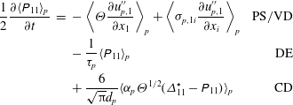 $$\begin{eqnarray}\displaystyle \begin{array}{@{}rclr@{}}\displaystyle \frac{1}{2}\frac{\partial \langle \unicode[STIX]{x1D617}_{11}\rangle _{p}}{\partial t}\ & =\ & \displaystyle -\left\langle {\it\Theta}\frac{\partial u_{p,1}^{\prime \prime }}{\partial x_{1}}\right\rangle _{p}+\left\langle {\it\sigma}_{p,1i}\frac{\partial u_{p,1}^{\prime \prime }}{\partial x_{i}}\right\rangle _{p} & \text{PS}/\text{VD}\\ \ & \ & -\,\displaystyle \frac{1}{{\it\tau}_{p}}\langle \unicode[STIX]{x1D617}_{11}\rangle _{p} & \text{DE}\\ \ & \ & +\,\displaystyle \frac{6}{\sqrt{{\rm\pi}}d_{p}}\langle {\it\alpha}_{p}{\it\Theta}^{1/2}({\it\Delta}_{11}^{\star }-\unicode[STIX]{x1D617}_{11})\rangle _{p} & \text{CD}\end{array} & & \displaystyle \nonumber\\ \displaystyle & & \displaystyle\end{eqnarray}$$
and
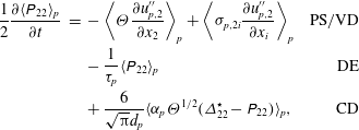 $$\begin{eqnarray}\displaystyle \begin{array}{@{}rclr@{}}\displaystyle \frac{1}{2}\frac{\partial \langle \unicode[STIX]{x1D617}_{22}\rangle _{p}}{\partial t}\ & =\ & \displaystyle -\left\langle {\it\Theta}\frac{\partial u_{p,2}^{\prime \prime }}{\partial x_{2}}\right\rangle _{p}+\left\langle {\it\sigma}_{p,2i}\frac{\partial u_{p,2}^{\prime \prime }}{\partial x_{i}}\right\rangle _{p} & \text{PS}/\text{VD}\\ \ & \ & -\,\displaystyle \frac{1}{{\it\tau}_{p}}\langle \unicode[STIX]{x1D617}_{22}\rangle _{p} & \text{DE}\\ \ & \ & +\,\displaystyle \frac{6}{\sqrt{{\rm\pi}}d_{p}}\langle {\it\alpha}_{p}{\it\Theta}^{1/2}({\it\Delta}_{22}^{\star }-\unicode[STIX]{x1D617}_{22})\rangle _{p}, & \text{CD}\end{array} & & \displaystyle \nonumber\\ \displaystyle & & \displaystyle\end{eqnarray}$$
where
 $$\begin{eqnarray}{\it\Delta}_{11}^{\star }={\textstyle \frac{1}{4}}(1+e)^{2}{\it\Theta}+{\textstyle \frac{1}{4}}(1-e)^{2}\unicode[STIX]{x1D617}_{11},\quad {\it\Delta}_{22}^{\star }={\textstyle \frac{1}{4}}(1+e)^{2}{\it\Theta}+{\textstyle \frac{1}{4}}(1-e)^{2}\unicode[STIX]{x1D617}_{22}.\end{eqnarray}$$
As previously discussed, the production of granular temperature
 $\langle \unicode[STIX]{x1D64B}\boldsymbol{ : }\boldsymbol{{\rm\nabla}}\boldsymbol{u}_{p}^{\prime \prime }\rangle _{p}$
in (2.42) shows up as a dissipation term in the particle-phase turbulent kinetic energy (2.40). The term for collisional dissipation (CD) requires further investigation.
In this work, fluid momentum is changed via the interphase exchange with the particles as well as gravity, and the flow remains statistically stationary by a source term added to the pressure gradient that prevents the development of a net mass flow rate. Applying the same assumptions used in simplifying the homogeneous RA particle-phase equations and taking into account the modified pressure gradient, the RA fluid-phase equations reduce to
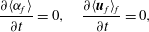 $$\begin{eqnarray}\frac{\partial \langle {\it\alpha}_{f}\rangle }{\partial t}=0,\quad \frac{\partial \langle \boldsymbol{u}_{f}\rangle _{f}}{\partial t}=0,\end{eqnarray}$$
(i.e.
 $\langle {\it\alpha}_{f}\rangle$
is constant and
 $\langle \boldsymbol{u}_{f}\rangle _{f}$
is null) and
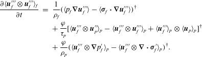 $$\begin{eqnarray}\displaystyle \frac{\partial \langle \boldsymbol{u}_{f}^{\prime \prime \prime }\otimes \boldsymbol{u}_{f}^{\prime \prime \prime }\rangle _{f}}{\partial t} & = & \displaystyle \frac{1}{{\it\rho}_{f}}(\langle p_{f}\boldsymbol{{\rm\nabla}}\boldsymbol{u}_{f}^{\prime \prime \prime }\rangle -\langle {\bf\sigma}_{f}\boldsymbol{\cdot }\boldsymbol{{\rm\nabla}}\boldsymbol{u}_{f}^{\prime \prime \prime }\rangle )^{\dagger }\nonumber\\ \displaystyle & & \displaystyle +\,\frac{{\it\varphi}}{{\it\tau}_{p}}[\langle \boldsymbol{u}_{f}^{\prime \prime \prime }\otimes \boldsymbol{u}_{p}^{\prime \prime }\rangle _{p}-\langle \boldsymbol{u}_{f}^{\prime \prime \prime }\otimes \boldsymbol{u}_{f}^{\prime \prime \prime }\rangle _{p}+\langle \boldsymbol{u}_{f}^{\prime \prime \prime }\rangle _{p}\otimes \langle \boldsymbol{u}_{p}\rangle _{p}]^{\dagger }\nonumber\\ \displaystyle & & \displaystyle +\,\frac{{\it\varphi}}{{\it\rho}_{p}}(\langle \boldsymbol{u}_{f}^{\prime \prime \prime }\otimes \boldsymbol{{\rm\nabla}}p_{f}^{\prime }\rangle _{p}-\langle \boldsymbol{u}_{f}^{\prime \prime \prime }\otimes \boldsymbol{{\rm\nabla}}\boldsymbol{\cdot }{\bf\sigma}_{f}^{\prime }\rangle _{p})^{\dagger }.\end{eqnarray}$$
Owing to the symmetry of the flow, the non-zero components of the PA fluid-phase Reynolds stress tensor are given by
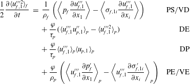 $$\begin{eqnarray}\displaystyle \begin{array}{@{}rclr@{}}\displaystyle \frac{1}{2}\frac{\partial \langle u_{f,1}^{\prime \prime \prime 2}\rangle _{f}}{\partial t}\ & =\ & \displaystyle \frac{1}{{\it\rho}_{f}}\left(\left\langle p_{f}\frac{\partial u_{f,1}^{\prime \prime \prime }}{\partial x_{1}}\right\rangle -\left\langle {\it\sigma}_{f,1i}\frac{\partial u_{f,1}^{\prime \prime \prime }}{\partial x_{i}}\right\rangle \right) & \text{PS}/\text{VD}\\ \ & \ & +\,\displaystyle \frac{{\it\varphi}}{{\it\tau}_{p}}(\langle u_{f,1}^{\prime \prime \prime }u_{p,1}^{\prime \prime }\rangle _{p}-\langle u_{f,1}^{\prime \prime \prime 2}\rangle _{p}) & \text{DE}\\ \ & \ & +\,\displaystyle \frac{{\it\varphi}}{{\it\tau}_{p}}\langle u_{f,1}^{\prime \prime \prime }\rangle _{p}\langle u_{p,1}\rangle _{p} & \text{DP}\\ \ & \ & +\,\displaystyle \frac{{\it\varphi}}{{\it\rho}_{p}}\left(\left\langle u_{f,1}^{\prime \prime \prime }\frac{\partial p_{f}^{\prime }}{\partial x_{1}}\right\rangle _{p}-\left\langle u_{f,1}^{\prime \prime \prime }\frac{\partial {\it\sigma}_{f,1i}^{\prime }}{\partial x_{i}}\right\rangle _{p}\right) & \text{PE}/\text{VE}\end{array} & & \displaystyle \nonumber\\ \displaystyle & & \displaystyle\end{eqnarray}$$
and
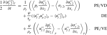 $$\begin{eqnarray}\displaystyle \begin{array}{@{}rclr@{}}\displaystyle \frac{1}{2}\frac{\partial \langle u_{f,2}^{\prime \prime \prime 2}\rangle _{f}}{\partial t}\ & =\ & \displaystyle \frac{1}{{\it\rho}_{f}}\left(\left\langle p_{f}\frac{\partial u_{f,2}^{\prime \prime \prime }}{\partial x_{2}}\right\rangle -\left\langle {\it\sigma}_{f,2i}\frac{\partial u_{f,2}^{\prime \prime \prime }}{\partial x_{i}}\right\rangle \right) & \text{PS}/\text{VD}\\ \ & \ & +\,\displaystyle \frac{{\it\varphi}}{{\it\tau}_{p}}(\langle u_{f,2}^{\prime \prime \prime }u_{p,2}^{\prime \prime }\rangle _{p}-\langle u_{f,2}^{\prime \prime \prime 2}\rangle _{p}) & \text{DE}\\ \ & \ & +\,\displaystyle \frac{{\it\varphi}}{{\it\rho}_{p}}\left(\left\langle u_{f,2}^{\prime \prime \prime }\frac{\partial p_{f}^{\prime }}{\partial x_{2}}\right\rangle _{p}-\left\langle u_{f,2}^{\prime \prime \prime }\frac{\partial {\it\sigma}_{f,2i}^{\prime }}{\partial x_{i}}\right\rangle _{p}\right). & \text{PE}/\text{VE}\end{array} & & \displaystyle \nonumber\\ \displaystyle & & \displaystyle\end{eqnarray}$$
It can be seen that fluid-phase turbulent kinetic energy is generated by the drag production (DP) term involving
 $\langle u_{f,1}^{\prime \prime \prime }\rangle _{p}$
, as opposed to the situation in single-phase turbulence, where it is produced by mean velocity gradients. The fluid–particle velocity covariance seen by the particles,
 $\langle \boldsymbol{u}_{f}^{\prime \prime \prime }\otimes \boldsymbol{u}_{p}^{\prime \prime }\rangle _{p}$
, appears in the drag exchange term and is thus an important mechanism for partitioning the turbulence kinetic energy between the two phases. The following section will present the numerical framework used to investigate these unclosed terms in the context of fully developed gravity-driven CIT.
3. Numerical approach
3.1. Configuration and simulation parameters
The volume-filtered fluid-phase equations presented in § 2.2.2 and the Lagrangian description of the particle phase given in § 2.2.1 are implemented in the framework of NGA (Desjardins et al.
Reference Desjardins, Blanquart, Balarac and Pitsch2008), a second-order, fully conservative computational fluid dynamics code tailored for turbulent flow computations. To assess the unclosed terms that appear in the RA equations from § 2.4, a range of simulations are conducted in the context of fully developed gravity-driven CIT. The independent dimensionless parameters that characterize homogeneous fluid–particle flows include the density ratio
 ${\it\rho}_{p}/{\it\rho}_{f}$
, the mean volume fraction
 $\langle {\it\alpha}_{p}\rangle$
and the mean particle Reynolds number defined as
 $$\begin{eqnarray}\mathit{Re}_{p}=\frac{\mathscr{V}d_{p}}{{\it\nu}_{f}},\end{eqnarray}$$
where the characteristic velocity
 $\mathscr{V}={\it\tau}_{p}g$
is the particle settling velocity in an undisturbed flow field when
 ${\it\rho}_{p}\gg {\it\rho}_{f}$
. Note that combining these non-dimensional numbers yields a Froude number
 $\mathit{Fr}={\it\rho}_{p}\mathit{Re}_{p}/(18{\it\rho}_{f})$
and the mean mass loading
 ${\it\varphi}$
. To obtain an a priori measure of the mesoscale features that arise due to the coupling between the phases, previous studies have introduced a characteristic length scale
 $\mathscr{L}={\it\tau}_{p}^{2}g$
in order to assess an appropriate domain size such that the results are unaffected by the periodic boundary conditions (see e.g. Agrawal et al.
Reference Agrawal, Loezos, Syamlal and Sundaresan2001; Igci et al.
Reference Igci, Andrews, Sundaresan, Pannala and O’Brien2008; Ozel et al.
Reference Ozel, Fede and Simonin2013). This length scale can be used to formulate a ‘mesoscale’ Reynolds number to characterize the fluid-phase inertia, i.e.
 $$\begin{eqnarray}\mathit{Re}_{f}=\frac{\mathscr{V}\mathscr{L}}{{\it\nu}_{f}}.\end{eqnarray}$$
The simulations presented in this work are solved on a triply periodic domain with gravity directed in the negative
 $x_{1}$
direction. The flows are made statistically stationary by a source term added to the pressure gradient in the fluid-phase momentum equation (2.10), which is computed dynamically in order to prevent the development of a net mass flow rate (i.e.
 $\langle \boldsymbol{u}_{f}\rangle _{f}=0$
). The particles are monodisperse and initially uniformly distributed throughout the domain of dimensions
 $3584d_{p}\times 896d_{p}\times 896d_{p}$
with a mesh size of
 $2048\times 512\times 512$
, corresponding to a uniform grid spacing of
 ${\rm\Delta}x=1.75d_{p}$
. The unclosed terms that arise in the RA transport equations are investigated for a range of
 $\mathit{Re}_{p}$
by keeping all parameters constant and modifying
 $g$
. A list of each simulation case and their corresponding parameters is given in table 1. Note that the Archimedes number,
 $\mathit{Ar}=({\it\rho}_{p}/{\it\rho}_{f}-1)d_{p}^{3}g/{\it\nu}^{2}$
, is commonly used in the literature to characterize gravity-driven fluid–particle flows (e.g. Noymer & Glicksman Reference Noymer and Glicksman2000; Ozel et al.
Reference Ozel, Fede and Simonin2013), and is related to our definition of the particle Reynolds number by
 $\mathit{Ar}=18\mathit{Re}_{p}$
, or equivalently to the square of the Galileo number defined in the introduction.
Fluid–particle parameters used in CIT simulations.
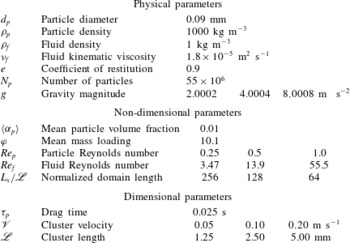
3.2. Implementation of the mesoscale equations
In this work, the Navier–Stokes equations are solved on a staggered grid with second-order spatial accuracy for both the convective and viscous terms. Time advancement is accomplished using the second-order accurate semi-implicit Crank–Nicolson scheme of Pierce (Reference Pierce2001). Momentum exchange between the phases is accounted for by the drag term
 $\mathbf{\mathscr{A}}$
given in (2.13). To account for unresolved fluid velocity fluctuations generated by the particles, a model derived by Gibilaro et al. (Reference Gibilaro, Gallucci, Di Felice and Pagliai2007) is used for the effective viscosity, given by
 $$\begin{eqnarray}{\it\nu}_{f}^{\star }=({\it\alpha}_{f}^{-2.8}-1){\it\nu}_{f}.\end{eqnarray}$$
We briefly note that contributions from
 ${\it\nu}_{f}^{\star }$
were found to be negligible compared to
 ${\it\nu}_{f}$
in the simulation cases considered in this work.
The particles are distributed among the processors based on the underlying domain decomposition of the fluid phase. For each particle, its position and velocity are solved using a second-order Runge–Kutta scheme. The collision force
 $\boldsymbol{F}_{c}$
that appears in (2.7) is modelled using a soft-sphere approach originally proposed by Cundall & Strack (Reference Cundall and Strack1979). When two particles come into contact, a repulsive force of particle
 $j$
on particle
 $i$
is created as
 $$\begin{eqnarray}\boldsymbol{f}_{c}^{(j\rightarrow i)}=\left\{\begin{array}{@{}ll@{}}-k{\it\delta}_{ij}\boldsymbol{n}_{ij}-{\it\eta}\boldsymbol{v}_{p}^{(ij)} & \text{if}\;d_{ij}<(d_{p}+{\it\lambda}),\\ 0 & \text{otherwise,}\end{array}\right.\end{eqnarray}$$
where
 $k$
and
 ${\it\eta}$
are the spring stiffness and the damping parameter, respectively,
 $\boldsymbol{n}_{ij}$
is the unit normal vector from particle
 $i$
to particle
 $j$
,
 ${\it\delta}_{ij}$
is the overlap between the particles, and the normal relative velocity between particles
 $i$
and
 $j$
is given by
 $$\begin{eqnarray}\boldsymbol{v}_{p}^{ij}=[(\boldsymbol{v}_{p}^{i}-\boldsymbol{v}_{p}^{j})\boldsymbol{\cdot }\boldsymbol{n}_{ij}]\boldsymbol{n}_{ij}.\end{eqnarray}$$
The collision force is computed when the distance between the centres of the particles
 $d_{ij}$
is less than the particle diameter
 $d_{p}$
and a force range
 ${\it\lambda}$
. The force range
 ${\it\lambda}$
is adjusted dynamically in order to recover the correct random close-packing limit when particles are in sustained contact, while providing a robust model for high-speed collisions (Capecelatro & Desjardins Reference Capecelatro and Desjardins2013a
). A model for the damping parameter is given by
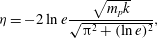 $$\begin{eqnarray}{\it\eta}=-2\ln e\frac{\sqrt{m_{p}k}}{\sqrt{{\rm\pi}^{2}+(\ln e)^{2}}},\end{eqnarray}$$
where
 $m_{p}={\rm\pi}{\it\rho}_{p}d_{p}^{3}/6$
is the particle mass. In this work, the restitution coefficient is taken to be
 $e=0.9$
. In order to limit inter-particle overlap during collisions, the simulation time step,
 ${\rm\Delta}t$
, is chosen such that particles cannot move more than one-tenth of their diameter per time step. The spring stiffness is related to the collision time,
 ${\it\tau}_{c}$
, according to
 $$\begin{eqnarray}k=m_{p}/{\it\tau}_{c}^{2}[{\rm\pi}^{2}+(\ln e)^{2}].\end{eqnarray}$$
To properly resolve the collisions without requiring an excessively small time step,
 ${\it\tau}_{c}$
is chosen to be an order of magnitude larger than
 ${\rm\Delta}t$
. Once each individual collision force is computed, the full collision force that particle
 $i$
experiences can be expressed as a sum of collisions with all other particles
 $j$
, i.e.
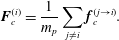 $$\begin{eqnarray}\boldsymbol{F}_{c}^{(i)}=\frac{1}{m_{p}}\mathop{\sum }_{j\neq i}\boldsymbol{f}_{c}^{(j\rightarrow i)}.\end{eqnarray}$$
Details on the parallel implementation of the Lagrangian particle tracking framework can be found in Capecelatro & Desjardins (Reference Capecelatro and Desjardins2013a ).
3.3. Two-way coupling
Coupling between the fluid phase and particles appears in the form of the volume fraction
 ${\it\alpha}_{p}$
and interphase exchange term
 $\mathbf{\mathscr{A}}$
. These terms are first computed at the location of each particle using information from the fluid, and are then transferred to the Eulerian mesh. To interpolate the fluid variables to the particle location, a second-order trilinear interpolation scheme is used. To extrapolate the particle data back to the Eulerian mesh, the volume-filtering approach used in the mathematical formulation of the fluid-phase mesoscale equations is applied. We begin by defining a filtering kernel
 $G$
with a characteristic length
 ${\it\delta}_{f}$
, such that
 $G(r)>0$
decreases monotonically with increasing
 $r$
, and is normalized such that it integrates to unity. Given a quantity
 $A^{(i)}(t)$
located at the centre of particle
 $i$
at time
 $t$
, and assuming
 $G$
does not vary significantly over the volume of the particle (i.e.
 ${\it\delta}_{f}\gg d_{p}$
), its Eulerian projection is given by
 $$\begin{eqnarray}\widetilde{{\it\alpha}}_{p}\widetilde{A}(\boldsymbol{x},t)\approx \mathop{\sum }_{i=1}^{N_{p}}A^{(i)}(t)G(|\boldsymbol{x}-\boldsymbol{x}_{p}^{(i)}|)V_{p},\end{eqnarray}$$
where
 $N_{p}$
is the total number of particles in a single realization of the flow and
 $V_{p}={\rm\pi}d_{p}^{3}/6$
is the particle volume. This expression replaces the discontinuous Lagrangian data with an Eulerian field that is a smooth function of the spatial coordinate
 $\boldsymbol{x}$
.
Note that (3.9) will only yield useful information if the spatial variations in the particle field can be decomposed into contributions on a scale comparable with the particle spacing and on a much larger scale corresponding to mesoscopic features in the flow (e.g. clusters), provided the filter size
 ${\it\delta}_{f}$
is within these scales. For ratios of
 ${\rm\Delta}x/d_{p}\approx 1$
, a brute-force implementation of (3.9) would require looping through a large number of cells for each particle, making this operation prohibitively expensive. Therefore, the filtering procedure is solved in two steps (Capecelatro & Desjardins Reference Capecelatro and Desjardins2013a
). First, the particle data are transferred to the nearest-neighbouring cells via trilinear extrapolation. The data are then diffused such that the final width of the filtering kernel is independent of the mesh size. In this work,
 $G$
is taken to be Gaussian with a characteristic length scale
 ${\it\delta}_{f}=8d_{p}$
, defined as the full width at half the height of the kernel. This value of
 ${\it\delta}_{f}$
was found to provide accurate solutions of the spatial distribution of the particle field in our previous work (Capecelatro et al.
Reference Capecelatro, Desjardins and Fox2014a
). To keep the cost low and ensure unconditional stability, the diffusion process is solved in a single implicit step by utilizing the approximate factorization scheme of Briley & McDonald (Reference Briley and McDonald1977).
3.4. Numerical approach for extracting multiphase statistics
We postulate that evaluating the multiphase statistics presented in § 2.4, in particular
 $k_{p}$
and
 $\langle {\it\Theta}\rangle _{p}$
, can be performed by introducing a separation of length scales when sampling the particle data. However, this requires validation, which is the purpose of this section. To accomplish this separation of length scales, we employ the spatial filtering procedure given by (3.9). The spatial filter is used in the first step of a two-step process for obtaining relevant statistics. The first step computes instantaneous Eulerian fields from Lagrangian particle data. The second step computes RA statistics from these Eulerian fields. In this section, we describe how the filter is defined such that the Eulerian turbulence statistics are computed accurately.
3.4.1. Influence of the filter size
The accuracy of the instantaneous results is dependent upon the sample size used when averaging, and therefore an appropriate value of the filter size
 ${\it\delta}_{f}$
is required. For example, averaging the instantaneous particle velocity in sample sizes much larger than the mean inter-particle distance, i.e.
 ${\it\delta}_{f}\gg d_{p}$
, will lead to
 $\boldsymbol{u}_{p}(\boldsymbol{x},t)\approx \langle \boldsymbol{u}_{p}\rangle _{p}$
. From the definition of
 $\boldsymbol{u}_{p}^{\prime \prime }$
, this would result in
 $k_{p}\approx 0$
and thus
 ${\it\kappa}_{p}$
only having contributions from
 $\langle {\it\Theta}\rangle _{p}$
. Likewise, averaging over a volume comparable to the particle diameter, i.e.
 ${\it\delta}_{f}\approx d_{p}$
, will lead to
 $\boldsymbol{u}_{p}(\boldsymbol{x},t)\approx \boldsymbol{v}_{p}^{(i)}(t)$
, and therefore
 ${\it\kappa}_{p}$
will only have contributions from
 $k_{p}$
. This behaviour is highlighted in figure 3, showing the influence of the filter size
 ${\it\delta}_{f}$
on the components of the particle-phase fluctuating energy for a single realization of fully developed CIT with
 $\mathit{Re}_{p}=1$
. Note that the mesh size limits the minimum amount of filtering, i.e.
 ${\it\delta}_{f}\leqslant {\rm\Delta}x$
implies that only the initial extrapolation step is performed (prior to filtering), and therefore
 ${\it\delta}_{f}=1.75d_{p}$
is the smallest possible filter size.
Influence of the filter size on the components of the fluctuating particle energy normalized by
 ${\it\kappa}_{p}$
:
 ${\it\kappa}_{p}$
(–○–),
 $k_{p}$
(–▵–),
 ${\textstyle \frac{3}{2}}\langle {\it\Theta}\rangle _{p}$
(–▫–). The particle field is taken from a single realization of
 $\mathit{Re}_{p}=1$
at steady state.
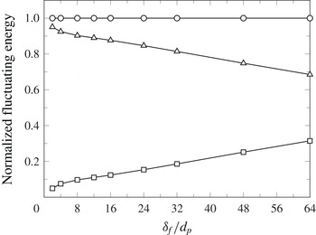
In order to obtain meaningful quantitative data from the simulations, the measured statistics should be independent of the averaging volume employed. It is clear from figure 3 that this requirement is not satisfied for the range of filter sizes considered. To alleviate this problem, we introduce an averaging volume that adapts to the local flow field, allowing for a sufficient number of particles to be sampled in dilute regions of the flow, while remaining optimally compact in dense clusters. Given an ensemble of identical (i.e. monodisperse) particles, and assuming that there are no sharp gradients in volume fraction, an averaging volume will sample
 $\mathscr{N}_{p}$
particles with a filter size
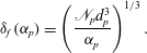 $$\begin{eqnarray}{\it\delta}_{f}({\it\alpha}_{p})=\left(\frac{\mathscr{N}_{p}d_{p}^{3}}{{\it\alpha}_{p}}\right)^{1/3}.\end{eqnarray}$$
Note that the computation of
 ${\it\alpha}_{p}$
requires
 ${\it\delta}_{f}$
, and therefore (3.10) is not known directly. As a result,
 ${\it\alpha}_{p}$
is first computed using an initially constant filter size
 ${\it\delta}_{f,0}$
, and the resulting volume fraction is applied to (3.10). This can be accomplished as an iterative process, as long as the resulting volume-fraction field converges with the number of iterations. The adaptive filter therefore depends on appropriate choices for the particle sample size
 $\mathscr{N}_{p}$
, the initial filter size
 ${\it\delta}_{f,0}$
and the number of iterations. Figure 4 shows the
 $L_{2}$
error norm from a single realization of fully developed CIT with
 $\mathit{Re}_{p}=1$
using (3.10) with
 $\mathscr{N}_{p}=10$
. The resulting volume-fraction fields are compared to a reference solution taken to be the filtered volume fraction after 11 iterations starting from an initially unfiltered field. Three key results can be inferred from figure 4. First,
 ${\it\alpha}_{p}$
converges rapidly to the reference solution with increasing iterations. Second, for the range of
 ${\it\delta}_{f,0}$
considered, the results converge to the same value and therefore the solution is independent of the choice of
 ${\it\delta}_{f,0}$
. Finally, it is observed that an initial filter size
 ${\it\delta}_{f,0}=8d_{p}$
yields the smallest errors and produces an error below 0.1 % after just one iteration. This value will be used throughout the remainder of this study. Thus, the only parameter required for extracting the Lagrangian statistics with the adaptive filter is
 $\mathscr{N}_{p}$
. The influence of
 $\mathscr{N}_{p}$
on the components of the particle-phase fluctuating energy
 ${\it\kappa}_{p}$
is shown in figure 5. The statistics were computed using a single iteration with
 ${\it\delta}_{f,0}=8d_{p}$
. The figure shows that the results are fairly constant for
 $10\leqslant \mathscr{N}_{p}\leqslant 100$
.
The
 $L_{2}$
error norm of the local volume-fraction field
 ${\it\alpha}_{p}$
in a single realization of
 $\mathit{Re}_{p}=1$
computed using the adaptive filter given by (3.10) with
 $\mathscr{N}_{p}=10$
. The
 ${\it\alpha}_{p}$
value is computed by recursively filtering the extrapolated Lagrangian data using an initial filter size
 ${\it\delta}_{f,0}=0$
(–○–),
 ${\it\delta}_{f,0}=2d_{p}$
(–▵–),
 ${\it\delta}_{f,0}=4d_{p}$
(–▫–),
 ${\it\delta}_{f,0}=8d_{p}$
(–
 $\times$
–) and
 ${\it\delta}_{f,0}=16d_{p}$
(–♢–).
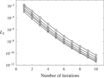
Influence of the particle sample size
 $\mathscr{N}_{p}$
used in the adaptive filter (3.10) on the components of the fluctuating energy normalized by
 ${\it\kappa}_{p}$
:
 ${\it\kappa}_{p}$
(–○–),
 $k_{p}$
(–▵–),
 ${\textstyle \frac{3}{2}}\langle {\it\Theta}\rangle _{p}$
(–▫–). The particle data are filtered using one iteration with
 ${\it\delta}_{f,0}=8d_{p}$
. The particle field is taken from a single realization of
 $\mathit{Re}_{p}=1$
at steady state.
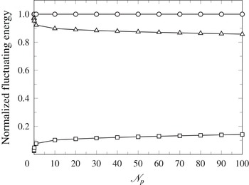
3.4.2. Validation of the adaptive filter
Lagrangian two-point statistics contain information on the spatial structure of the particle field and are useful in describing the multiphase dynamics in fully developed CIT. Because two-point statistics are computed as a continuous function of particle pair separation, a specific averaging volume is not required, and thus they can be used to assess the accuracy of the filtering procedure in extracting the multiphase statistics. An important statistical measure of the spatial distribution of particles is the radial distribution function (RDF), defined as the number of particle pairs found at a given separation normalized by the expected number of pairs found in a homogeneous distribution (McQuarrie Reference McQuarrie1976), which can be expressed as
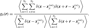 $$\begin{eqnarray}g_{0}(\boldsymbol{r})=\frac{\displaystyle \left\langle \mathop{\sum }_{m=1}^{N_{p}}\mathop{\sum }_{n\neq m}^{N_{p}}{\it\delta}(\boldsymbol{x}-\boldsymbol{x}_{p}^{(m)}){\it\delta}(\boldsymbol{x}+\boldsymbol{r}-\boldsymbol{x}_{p}^{(n)})\right\rangle }{\displaystyle \left\langle \mathop{\sum }_{m=1}^{N_{p}}{\it\delta}(\boldsymbol{x}-\boldsymbol{x}_{p}^{(m)})\right\rangle \left\langle \mathop{\sum }_{m=1}^{N_{p}}{\it\delta}(\boldsymbol{x}+\boldsymbol{r}-\boldsymbol{x}_{p}^{(m)})\right\rangle },\end{eqnarray}$$
where
 ${\it\delta}$
is the Dirac delta function and
 $\boldsymbol{r}=[r_{1},r_{2},r_{3}]^{\text{T}}$
is the separation between two particles
 $n\neq m$
with
 $r=|\boldsymbol{r}|\geqslant d_{p}$
. With this definition,
 $g_{0}=1$
represents a homogeneous distribution of particles, and
 $g_{0}>1$
implies clustering. Similarly, we define the two-particle velocity correlation as
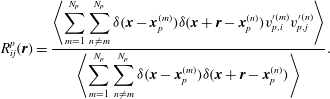 $$\begin{eqnarray}R_{ij}^{p}(\boldsymbol{r})=\frac{\displaystyle \left\langle \mathop{\sum }_{m=1}^{N_{p}}\mathop{\sum }_{n\neq m}^{N_{p}}{\it\delta}(\boldsymbol{x}-\boldsymbol{x}_{p}^{(m)}){\it\delta}(\boldsymbol{x}+\boldsymbol{r}-\boldsymbol{x}_{p}^{(n)})v_{p,i}^{\prime (m)}v_{p,j}^{\prime (n)}\right\rangle }{\displaystyle \left\langle \mathop{\sum }_{m=1}^{N_{p}}\mathop{\sum }_{n\neq m}^{N_{p}}{\it\delta}(\boldsymbol{x}-\boldsymbol{x}_{p}^{(m)}){\it\delta}(\boldsymbol{x}+\boldsymbol{r}-\boldsymbol{x}_{p}^{(n)})\right\rangle }.\end{eqnarray}$$
Owing to the homogeneity of the flows considered in this work, (3.11) and (3.12) are functions of the pair separation only, but in the presence of gravity, the statistics may exhibit strong anisotropy and therefore depend strongly on the directionality of
 $\boldsymbol{r}$
. Note that, when computing the two-particle velocity correlation, only the correlated contribution of the particle-phase velocity is retained after averaging (Février et al.
Reference Février, Simonin and Squires2005), and thus only contributions from the PA turbulent kinetic energy
 $k_{p}$
are captured.
Comparison between Lagrangian and filtered Eulerian RDFs computed in the (a) streamwise and (b) spanwise directions. Symbols correspond to two-point Lagrangian statistics from
 $\mathit{Re}_{p}=0.25$
(○),
 $\mathit{Re}_{p}=0.5$
(▵) and
 $\mathit{Re}_{p}=1$
(▫). Lines represent two-point Eulerian statistics with
 ${\it\delta}_{f,0}=8d_{p}$
and
 $\mathscr{N}_{p}=10$
from
 $\mathit{Re}_{p}=0.25$
(——),
 $\mathit{Re}_{p}=0.5$
(– – –) and
 $\mathit{Re}_{p}=1$
(
 $\cdots \cdots$
).
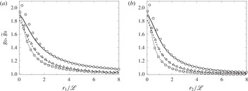
Starting from the one-particle probability distribution function, Février et al. (Reference Février, Simonin and Squires2005) showed that, for dilute (non-collisional) suspensions of inertial particles in isotropic turbulence, two-point Eulerian statistics can be computed by introducing averages conditioned on a given fluid-flow realization, where the Eulerian RDF is given by
 $$\begin{eqnarray}\widetilde{g}_{0}(\boldsymbol{r})=\frac{\langle {\it\alpha}_{p}(\boldsymbol{x},t){\it\alpha}_{p}(\boldsymbol{x}+\boldsymbol{r},t)\rangle }{\langle {\it\alpha}_{p}(\boldsymbol{x},t)\rangle \langle {\it\alpha}_{p}(\boldsymbol{x}+\boldsymbol{r},t)\rangle }\end{eqnarray}$$
and the Eulerian two-point velocity correlation can be written as
 $$\begin{eqnarray}\widetilde{R}_{ij}^{p}(\boldsymbol{r})=\frac{\langle {\it\alpha}_{p}(\boldsymbol{x},t){\it\alpha}_{p}(\boldsymbol{x}+\boldsymbol{r},t)u_{p,i}^{\prime \prime }(\boldsymbol{x},t)u_{p,j}^{\prime \prime }(\boldsymbol{x}+\boldsymbol{r},t)\rangle }{\langle {\it\alpha}_{p}(\boldsymbol{x},t){\it\alpha}_{p}(\boldsymbol{x}+\boldsymbol{r},t)\rangle }.\end{eqnarray}$$
A key result found in the work by Février et al. (Reference Février, Simonin and Squires2005) is that the correlated Eulerian contribution to the particle-phase velocity accounts completely for the two-point Lagrangian statistics, such that
 $g_{0}=\widetilde{g}_{0}$
and
 $R_{ij}^{p}=\widetilde{R}_{ij}^{p}$
. Capecelatro et al. (Reference Capecelatro, Desjardins and Fox2014a
) extended this approach to the moderately dilute collisional fluid–particle flows considered in this work. In the limit of small pair separation, the Eulerian two-point statistics are given by
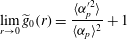 $$\begin{eqnarray}\lim _{r\rightarrow 0}\widetilde{g}_{0}(r)=\frac{\langle {\it\alpha}_{p}^{\prime 2}\rangle }{\langle {\it\alpha}_{p}\rangle ^{2}}+1\end{eqnarray}$$
and
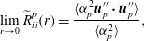 $$\begin{eqnarray}\lim _{r\rightarrow 0}\widetilde{R}_{ii}^{p}(r)=\frac{\langle {\it\alpha}_{p}^{2}\boldsymbol{u}_{p}^{\prime \prime }\boldsymbol{\cdot }\boldsymbol{u}_{p}^{\prime \prime }\rangle }{\langle {\it\alpha}_{p}^{2}\rangle },\end{eqnarray}$$
with implied summation over the repeated index
 $i$
. Comparisons between the two-point Lagrangian correlations (3.11)–(3.12) and two-point Eulerian statistics (3.13)–(3.14) computed using (3.10) with
 $\mathscr{N}_{p}=10$
are provided in figures 6 and 7, demonstrating the capability of the adaptive filter to reproduce the instantaneous spatial distribution of particle position and velocity for the range of
 $\mathit{Re}_{p}$
considered in this study. The largest discrepancies exist in the computation of the RDF at small pair separations, though overall the filtering approach yields excellent agreement with the two-point Lagrangian statistics. Note that, in the limit of pair separation
 $\boldsymbol{r}\rightarrow 0$
, the two-point velocity correlations remain smaller than
 ${\it\kappa}_{p}$
, indicating the existence of a finite granular temperature associated with the spatially uncorrelated particle velocity component. In this limit of small pair separation, the two-point correlations become independent of the measurement direction, and thus
 $g_{0}$
and
 $R_{ij}^{p}$
are functions only of
 $r$
.
Comparison between Lagrangian and filtered Eulerian two-particle velocity correlations computed in the (a) streamwise and (b) spanwise directions. Symbols correspond to two-point Lagrangian statistics from
 $\mathit{Re}_{p}=0.25$
(○),
 $\mathit{Re}_{p}=0.5$
(▵) and
 $\mathit{Re}_{p}=1$
(▫). Lines represent two-point Eulerian statistics with
 ${\it\delta}_{f,0}=8d_{p}$
and
 $\mathscr{N}_{p}=10$
from
 $\mathit{Re}_{p}=0.25$
(——),
 $\mathit{Re}_{p}=0.5$
(– – –) and
 $\mathit{Re}_{p}=1$
(
 $\cdots \cdots$
).
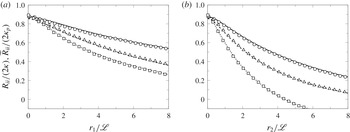
To assess the accuracy of the adaptive filter in evaluating the spatial distribution of particles in an Eulerian frame, the following errors are defined:
 $$\begin{eqnarray}{\it\epsilon}_{g}=\left.\left|\lim _{r\rightarrow 0}\widetilde{g}_{0}(r)-\lim _{r\rightarrow 0}g_{0}(r)\right|\,\right/\lim _{r\rightarrow 0}g_{0}(r)\end{eqnarray}$$
and
 $$\begin{eqnarray}{\it\epsilon}_{R}=\left.\left|\lim _{r\rightarrow 0}\widetilde{R}_{ii}^{p}(r)-\lim _{r\rightarrow 0}R_{ii}^{p}(r)\right|\,\right/\lim _{r\rightarrow 0}R_{ii}^{p}(r).\end{eqnarray}$$
The corresponding errors are provided in figure 8. In general, the smallest errors are associated with
 $\mathit{Re}_{p}=1$
, and increase with decreasing
 $\mathit{Re}_{p}$
. It is seen that the adaptive filter provides a better solution to the velocity distribution (
 $R_{ii}^{p}$
) compared to the local particle distribution
 $g_{0}$
, with
 $\mathscr{N}_{p}=10$
providing overall the minimum error. It is important to note that, in the densest regions of the flow,
 $\mathscr{N}_{p}\approx 3$
yields a filter size
 ${\it\delta}_{f}\approx {\rm\Delta}x$
, and thus a portion of the error associated with
 $\mathscr{N}_{p}<3$
is attributed to the initial extrapolation to the mesh and does not reflect the performance of the adaptive filter.
Validation of the adaptive spatial filter in extracting local instantaneous information from the Lagrangian particles to the Eulerian mesh. Comparisons between Lagrangian and filtered Eulerian radial distribution functions (a) and two-point velocity correlations (b) at zero pair separations.
 $\mathit{Re}_{p}=0.25$
(○),
 $\mathit{Re}_{p}=0.5$
(▵) and
 $\mathit{Re}_{p}=1$
(▫).
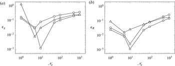
4. Results and discussion
4.1. Visualizations of instantaneous fully developed CIT
The simulations are run until the initial transient is complete and the flows reach a statistically stationary state. Owing to the non-trivial coupling between the phases, the transients were observed to persist longer than
 $80{\it\tau}_{p}$
. Once a statistical steady state has been reached, results are measured at each computational time step (
 ${\rm\Delta}t=3.25\times 10^{-4}\,{\it\tau}_{p}$
,
 $5.2\times 10^{-4}\,{\it\tau}_{p}$
and
 $8.0\times 10^{-4}\,{\it\tau}_{p}$
for
 $\mathit{Re}_{p}=0.25$
, 0.5 and 1.0, respectively), over a duration of approximately
 $10{-}15\,{\it\tau}_{p}$
. As shown in figure 9, the resulting particle field is highly non-uniform, with significant segregation in volume fraction. The corresponding fields of fluid velocity are shown in figure 10. The fluid is observed to be entrained by the clusters, leading to strong vertical velocities in dilute regions of the flow, indicative of jet bypassing. Furthermore, the magnitude of the local fluid-phase velocity, normalized by their respective terminal velocities, is seen to decrease with increasing
 $\mathit{Re}_{p}$
.
Instantaneous fields of particle volume fraction in a two-dimensional plane of the fully developed CIT with (a)
 $\mathit{Re}_{p}=0.25$
, (b)
 $\mathit{Re}_{p}=0.5$
and (c)
 $\mathit{Re}_{p}=1$
.
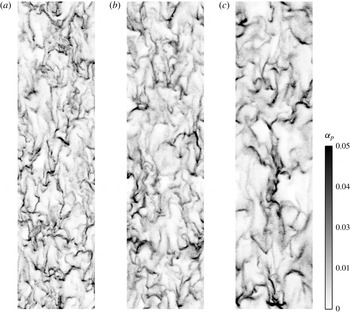
Instantaneous fields of fluid velocity in a two-dimensional plane of the fully developed CIT with (a)
 $\mathit{Re}_{p}=0.25$
, (b)
 $\mathit{Re}_{p}=0.5$
and (c)
 $\mathit{Re}_{p}=1$
. Iso-countours of
 ${\it\alpha}_{p}=3\langle {\it\alpha}_{p}\rangle$
are shown in black.
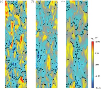
Relative contributions to kinetic energy production and dissipation.
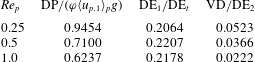
4.2. Overall kinetic energy balance
The unclosed terms appearing in the RA equations are evaluated via the adaptive spatial filter introduced in § 3.4, and each equation is analysed in detail in § 4.4. Based on the magnitude of the terms in the RA equations, we can identify the overall kinetic energy balance for CIT shown in figure 11. In this balance, the drag production (DP) is proportional to
 $\langle u_{f,1}^{\prime \prime \prime }\rangle _{p}$
, which is zero in the absence of clusters. As in single-phase turbulence, the viscous dissipation (VD) results from the resolved small-scale velocity fluctuations in the fluid phase. In contrast, the drag exchange terms represent two separate phenomena: (i) viscous dissipation of unresolved fluid velocity fluctuations (
 $\text{DE}_{2}$
), e.g. in the viscous boundary layers around individual particles; and (ii) energy transferred to the particles at the fluid–particle interface (
 $\text{DE}_{1}$
). As described by Sundaram & Collins (Reference Sundaram and Collins1999), the unresolved dissipation arises in the point-particle model due to the difference between the fluid velocity at the particle location and the particle velocity. Denoting the sum of the two contributions as
 $\text{DE}_{t}$
, in table 2 we observe that the relative contribution of the interphase energy exchange (
 $\text{DE}_{1}/\text{DE}_{t}$
) is approximately 22 % for all
 $\mathit{Re}_{p}$
. Furthermore, the ratio of the resolved to unresolved viscous dissipation is less than 6 % and decreases with increasing
 $\mathit{Re}_{p}$
. It is interesting to note in table 2 that the fraction of the total kinetic energy production going to DP is largest for the smallest
 $\mathit{Re}_{p}$
. Presumably this fraction would approach unity as
 $\mathit{Re}_{p}$
approaches zero if the clusters were fully developed. Numerically, this conjecture would be difficult to verify starting from uniformly distributed particles because the transient to fully developed clusters increases with decreasing
 $\mathit{Re}_{p}$
.
Schematic of the kinetic energy balance in CIT. Kinetic energy is produced by particles falling due to gravity. In the absence of clustering, mean kinetic energy production is balanced by mean drag (
 ${\it\phi}u_{p}^{2}/{\it\tau}_{p}$
with
 $u_{p}=\mathscr{V}$
), which generates viscous heating of the fluid (i.e. increases the thermodynamic temperature
 $T_{f}$
). In fully developed CIT, drag production (DP) generates fluid-phase turbulent kinetic energy (
 $k_{f}$
), which is dissipated to heat the fluid directly by viscous dissipation (VD) and indirectly by drag exchange (
 $\text{DE}_{2}$
). The remaining fraction of the fluid-phase turbulent kinetic energy is transferred to the particle phase by drag exchange (
 $\text{DE}_{1}$
), and is subsequently dissipated to heat the fluid through the fluctuating drag (
 ${\it\kappa}_{p}/{\it\tau}_{p}$
).
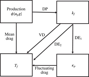
As will be shown in the following section, owing to the formation of clusters, in fully developed CIT the average falling velocity of particles (
 $|\langle u_{p,1}\rangle _{p}|$
) increases significantly relative to the particle falling velocity without clustering (
 $\mathscr{V}$
). Some of this additional particle-phase kinetic energy is dissipated by mean drag, while the remainder is transferred to fluid-phase turbulent kinetic energy through drag production. In the fluid phase, nearly 80 % of the turbulent kinetic energy is dissipated by unresolved viscous dissipation (i.e.
 $\text{DE}_{2}$
) and the rest is transferred to particle-phase fluctuation energy. As we shall see in § 4.4, only a very small fraction of the particle-phase fluctuation energy is dissipated due to inelastic particle–particle collisions.
4.3. One-point statistics
Having established the overall kinetic energy balance for fully developed CIT, we now turn our attention to specific one-point statistics for the fluid and particle phases. In table 3, we present statistics for the fluid phase for each value of
 $\mathit{Re}_{p}$
. First, note that, although the scaled value of
 $k_{f}$
decreases with
 $\mathit{Re}_{p}$
, the anisotropy between the vertical and horizontal components is nearly constant. Second, the fluid velocity statistics exhibit non-Gaussian behaviour. The vertical velocity component has significant positive skewness, while its kurtosis is close to the Gaussian value of 3. The horizontal component has negligible skewness (as would be expected due to symmetry), but with a large kurtosis. The non-Gaussian behaviour of the one-point fluid velocity statistics is confirmed from the one-point p.d.f.s shown in figure 12. Details on the formulation of the one-point p.d.f.s can be found in appendix A. Finally, note that these p.d.f.s exhibit reasonably good collapse for all
 $\mathit{Re}_{p}$
.
The p.d.f.s of the (a) streamwise and (b) spanwise components of PA fluid-phase velocity from fully developed CIT with
 $\mathit{Re}_{p}=0.25$
(——),
 $\mathit{Re}_{p}=0.5$
(– – –) and
 $\mathit{Re}_{p}=1$
(
 $\cdots \cdots$
) compared to a Gaussian distribution (▵).
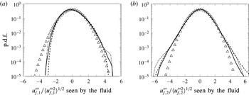
Fluid-phase velocity statistics.
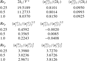
The one-point statistics for the particle-phase volume fraction are given in table 4. The corresponding one-point p.d.f.s are shown in figure 13. For a homogeneous distribution of particles, devoid of any clustering, the p.d.f. is given by the discrete Poisson distribution (Squires & Eaton Reference Squires and Eaton1991; Eaton & Fessler Reference Eaton and Fessler1994), which takes the form
 $$\begin{eqnarray}f_{p}(N)=\frac{\overline{N}^{N}\text{e}^{-\overline{N}}}{N!},\end{eqnarray}$$
where
 $N$
is the observed number of particles in a given sample, and
 $\overline{N}$
is the average particle number. In figure 13, the volume-fraction p.d.f.s display a higher probability of local regions empty of particles, as well as local regions of higher solid fraction, compared to (4.1). Although the characteristic cluster size appears to increase with
 $\mathit{Re}_{p}$
in figure 9, the distribution of volume fraction is shown to be unaffected by the Reynolds number. Using the mean and variance particle volume fraction extracted from
 $\mathit{Re}_{p}=1$
, the forms of the p.d.f.s are seen to closely resemble a lognormal distribution, indicating a potential opportunity for future modelling efforts (see appendix B).
The p.d.f. of particle volume fraction from single realizations of the fully developed CIT with
 $\mathit{Re}_{p}=0.25$
(——),
 $\mathit{Re}_{p}=0.5$
(– – –) and
 $\mathit{Re}_{p}=1$
(
 $\cdots \cdots$
), corresponding to lognormal (○) and Poisson (▵) distributions.
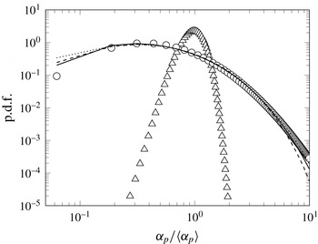
In table 5, we present statistics for the particle phase for all values of
 $\mathit{Re}_{p}$
. First, we observe that the fall velocity
 $|\langle u_{p,1}\rangle _{p}|$
is more than twice as large as the reference velocity
 $\mathscr{V}$
due to the formation of clusters. Second, note that, as for the fluid, the scaled value of
 ${\it\kappa}_{p}$
decreases with
 $\mathit{Re}_{p}$
, but the anisotropy between the vertical and horizontal components is nearly constant. The same is true for
 $k_{p}$
and
 $\langle {\it\Theta}\rangle _{p}$
. Note also that, while the anisotropy in the correlated components (e.g.
 $\langle u_{p,1}^{\prime \prime 2}\rangle _{p}$
) is larger than in the uncorrelated components (e.g.
 $\langle \unicode[STIX]{x1D617}_{11}\rangle _{p}$
), the latter is too large to be approximated as isotropic. Next, the one-point p.d.f.s of the correlated components of the particle velocity statistics are shown in figure 14, displaying a reasonably good collapse for all
 $\mathit{Re}_{p}$
. While the vertical component is observed to be positively skewed, the overall behaviour of the correlated particle-phase velocity statistics is close to Gaussian. In contrast, the velocity statistics for the uncorrelated components of the particle velocity are significantly non-Gaussian, as seen by the large third-order moments in table 5, as well as the one-point p.d.f.s shown in figure 15. Sundaram & Collins (Reference Sundaram and Collins1997) report a non-Gaussian p.d.f. for the relative particle velocity in isotropic, particle-laden turbulence. This observation is consistent with figure 15 because the relative particle velocity will be mainly due to the spatially uncorrelated particle velocity field represented by
 ${\bf\delta}\boldsymbol{v}_{p}$
. It is evident from the exponential tails of the p.d.f.s that the uncorrelated components retain a strong imprint of their production terms from the correlated components that is not erased by particle–particle collisions.
Particle-phase volume-fraction statistics.
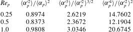
Particle-phase velocity statistics.
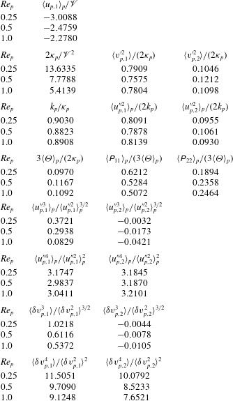
The p.d.f.s of the (a) streamwise and (b) spanwise components of PA particle-phase velocity from fully developed CIT with
 $\mathit{Re}_{p}=0.25$
(——),
 $\mathit{Re}_{p}=0.5$
(– – –) and
 $\mathit{Re}_{p}=1$
(
 $\cdots \cdots$
) compared to a Gaussian distribution (▵).
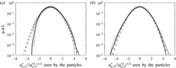
The p.d.f.s of the (a) streamwise and (b) spanwise components of velocity residual
 ${\bf\delta}\boldsymbol{v}_{p}$
used in defining the particle pressure tensor
 $\unicode[STIX]{x1D64B}$
and granular temperature
 ${\it\Theta}$
, with
 $\mathit{Re}_{p}=0.25$
(——),
 $\mathit{Re}_{p}=0.5$
(– – –) and
 $\mathit{Re}_{p}=1$
(
 $\cdots \cdots$
) compared to a Gaussian distribution (▵).
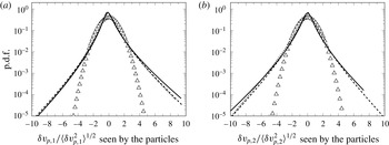
As described in appendix A, it is straightforward to compute statistics for the fluid phase seen by the particles from the Eulerian fields. Thus, in table 6, selected fluid and fluid–particle statistics seen by the particles are presented. First, the normalized mean fluid velocity seen by the particles
 $|\langle u_{f,1}\rangle _{p}|/\mathscr{V}$
can be seen to decrease with
 $\mathit{Re}_{p}$
. As discussed earlier, a non-zero value for
 $\langle u_{f,1}\rangle _{p}$
is a direct result of particle clustering and the fact that clusters entrain the fluid in their vicinity due to momentum coupling. Second, note that the fluid-phase turbulence kinetic energy seen by the particles
 $k_{f@p}$
is nearly the same as
 $k_{f}$
; however, its components are more anisotropic due to the drag production term. Third, the fluid–particle kinetic energy
 $k_{fp}$
is approximately equal to
 $0.87\sqrt{k_{f}k_{p}}$
for all
 $\mathit{Re}_{p}$
, and the anisotropy of its components is nearly the same as for
 $k_{f}$
and
 $k_{p}$
. Finally, the fluid velocity statistics seen by the particles are super-Gaussian, which is confirmed by the one-point p.d.f.s shown in figure 16.
Fluid-phase turbulence statistics seen by particles.
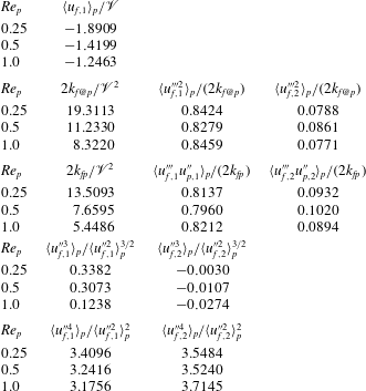
The p.d.f.s of the (a) streamwise and (b) spanwise components of fluid velocity seen by the particles from fully developed CIT with
 $\mathit{Re}_{p}=0.25$
(——),
 $\mathit{Re}_{p}=0.5$
(– – –) and
 $\mathit{Re}_{p}=1$
(
 $\cdots \cdots$
) compared to a Gaussian distribution (▵).
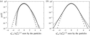
In summary, in this section we have presented one-point statistics for the principal quantities of interest in fully developed CIT. From these statistics, we see that the momentum coupling between the two phases leads to significant differences from the behaviour observed for very dilute systems with one-way coupling (Minier & Peirano Reference Minier and Peirano2001). Most importantly, owing to momentum coupling, the particle phase spontaneously organizes into clusters (or, equivalently, volume-fraction fluctuations with a near lognormal p.d.f.) that significantly increases the mean particle velocity relative to an isolated particle in an undisturbed flow. In turn, the increased mean particle velocity generates a drag production term for turbulent kinetic energy in the fluid phase that is highly anisotropic. Furthermore, the fluid-phase velocity p.d.f.s are non-Gaussian. Owing to the compressibility of the particle phase, the uncorrelated components of the particle-phase velocity statistics are highly non-Gaussian. This situation can be contrasted with the one-way coupling case where in the homogeneous limit all of the velocity statistics are nearly Gaussian (Minier & Peirano Reference Minier and Peirano2001). These differences would suggest that a predictive p.d.f. model for CIT must explicitly account for the compressibility of the particle phase. Finally, it is noteworthy that the uncorrelated particle velocity statistics (i.e.
 $\unicode[STIX]{x1D64B}$
) are significantly anisotropic in our simulations. At least for systems with moderately low mean particle volume fractions for which particle–particle collisions are too infrequent to ensure that
 $\unicode[STIX]{x1D64B}$
is nearly isotropic, this fact comprises the effectiveness of traditional kinetic-theory closures for
 $\unicode[STIX]{x1D64B}$
wherein a constitutive equation is used to represent
 ${\bf\sigma}_{p}$
.
4.4. Turbulence budgets
Having provided an overall analysis of the kinetic energy budget for CIT in § 4.2, we now turn to a detailed analysis of the individual RA balance equations derived in § 2.4. In particular, we compute each term in the steady-state balance equations for homogeneous gravity-driven flow and use the notation introduced in § 2.4 to denote each term. From tables 7–11, it can be noticed that, after time averaging the various RA terms, some of the equations remain unbalanced. Defining an error as the residual normalized by the largest term appearing in the equation, it is seen that the RA balance equations for
 $\langle u_{p,1}\rangle _{p}$
and
 $k_{f}$
exhibit errors below 11 %, while the particle-phase energy budgets (
 $k_{p}$
and
 $\langle {\it\Theta}\rangle _{p}$
) are observed to have errors as large as 50 %. The errors associated with the particle-phase balance equations are attributed to inconsistencies with the Lagrangian reconstruction of the various Eulerian terms, in particular the terms involving gradients of the particle-phase Eulerian fields. Meanwhile, the relative importance of the key terms appearing in the RA equations are captured and provide useful insight on the energy exchange in CIT.
4.4.1. Fluid-phase momentum budget
In order to reach statistical stationarity in the flows, a source terms is added to the fluid-phase momentum equation in the form of a modified pressure gradient. As a result, the fluid-phase momentum balance is forced to zero. It is important to note that the time-dependent nature of the forcing can play a role on the cluster dynamics. However, for each simulation, fluctuations in the pressure gradient forcing were observed to remain below
 $\pm 2\,\%$
of its mean value at steady state, indicating that the source term is essentially constant in time and thus does not impact the statistics reported in this paper.
4.4.2. Particle-phase momentum budget
From table 7, the particle-phase momentum involves a balance between the drag exchange (DE) term and gravity. Owing to the large solid-to-fluid density ratio, the viscous exchange (VE) and pressure exchange (PE) terms are very small. Thus, the PA fluid-phase velocity seen by the particles is well represented by
 $\langle u_{f,1}\rangle _{p}=\langle u_{p,1}\rangle _{p}+{\it\tau}_{p}g$
, as predicted by (2.43) in the limit
 ${\it\rho}_{p}\gg {\it\rho}_{f}$
at steady state.
Particle-phase momentum budget.
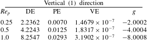
4.4.3. Fluid-phase Reynolds stress budgets
The fluid-phase Reynolds stress budgets are presented in table 8. Again, the PE and VE contributions are very small due to the large density ratio. In the vertical direction, drag production (DP) is nearly balanced by drag exchange (DE) and pressure strain (PS). In comparison, viscous dissipation (VD) is small. Note, however, that PS is one order of magnitude smaller than DP, and thus is unable to significantly reduce the anisotropy in the fluid-phase Reynolds stresses. In the horizontal direction, PS is the main production term resulting from the weak reorientation of vertical to horizontal Reynolds stress. PS is balanced mainly by DE, with a relatively small contribution from VD. The balance for
 $k_{f}$
is dominated by production due to DP and dissipation due to DE. The turbulent dissipation rate VD is approximately two orders of magnitude smaller than DE. Note that PS for
 $k_{f}$
is non-zero in CIT because the fluid phase is weakly compressible. Compared to single-phase turbulence, the principal production and dissipation mechanisms for
 $k_{f}$
in CIT are completely different (i.e. DP in place of mean shear and DE in place of VD).
Fluid-phase Reynolds stress budgets.
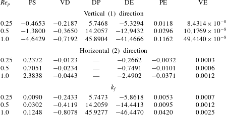
4.4.4. Particle-phase Reynolds stress budgets
The particle-phase Reynolds stress budgets are presented in table 9. Again, PE and VE are very small due to the large density ratio. In the vertical direction, production due to DE is nearly balanced by VD and PS. Note that PS is significantly smaller than DE, and thus is unable to significantly reduce the anisotropy in the particle-phase Reynolds stresses. In the horizontal direction, DE and PS contribute roughly equally to production, which is balanced mainly by VD. Compared to the fluid phase, all of the terms in the budgets are two orders of magnitude smaller in the particle phase. The balance for
 $k_{p}$
has production due to DE and dissipation mainly due to VD. PS is again non-zero because the particle phase is compressible. Overall, the budget for
 $k_{p}$
is similar to single-phase turbulence with a balance between DE and VD. However, compared to
 $k_{f}$
, the production of
 $k_{p}$
is nearly two orders of magnitude smaller.
Particle-phase Reynolds stress budgets.
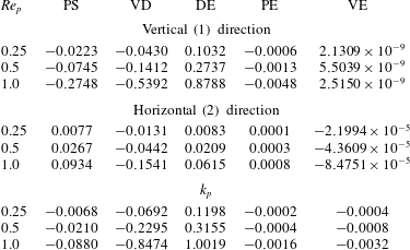
4.4.5. Particle-phase stress tensor budgets
The particle-phase stress tensor budgets are presented in table 10. Production of the vertical component is due to PS and VD, whereas dissipation is due to DE and reorientation (and a small amount of dissipation) to CD. In contrast, PS is a dissipation term for the horizontal component, along with DE. Moreover, owing to reorientation by particle–particle collisions, CD is a production term. Note that, because the terms in the balance equations for the vertical and horizontal components have equivalent magnitudes, the particle-phase stress tensor is less anisotropic than the Reynolds stresses. However, we can also note that the particle–particle collisions are too infrequent to make the stress tensor nearly isotropic. The balance equation for the granular temperature exhibits a balance between production due to VD and dissipation due to DE. In comparison, the production due to PS and the dissipation due to CD are one order of magnitude smaller. From this observation, we can conclude that inelastic collisions do not play a significant role in the overall kinetic energy balance.
Particle-phase stress tensor budgets.
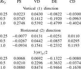
4.4.6. Fluctuating energy budgets
By combining the appropriate terms in the individual energy budgets, the fluctuating energy budgets given in table 11 can be established. Consistent with our previous observations, PE and VE are very small and can be neglected. For the correlated kinetic energy, PS is also small, and hence production due to DP is balanced by dissipation due to DE and, to a smaller extent, VD. Recalling that particle-phase VD leads to the production of granular temperature, we see that in the total fluctuating energy balance DP is balanced by DE, where the latter is now larger due to the added contribution of granular temperature DE. These observations are summarized in the overall kinetic energy flow diagram shown in figure 11. A simple model for the Reynolds stresses, consistent with the turbulence budgets, is given in appendix C.
Fluctuating energy budgets.
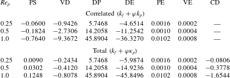
Vertical fluid velocity conditioned on
 ${\it\alpha}_{p}$
from single realizations of fully developed CIT with
 $\mathit{Re}_{p}=0.25$
(——),
 $\mathit{Re}_{p}=0.5$
(– – –) and
 $\mathit{Re}_{p}=1$
(
 $\cdots \cdots$
).
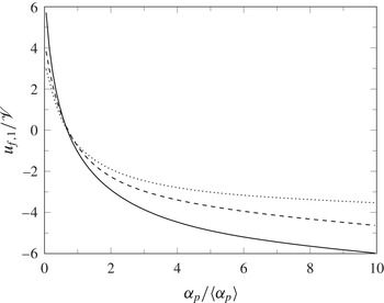
4.5. Conditional statistics
As shown earlier, the particle-phase volume fraction has a one-point p.d.f. close to lognormal and exhibits large fluctuations about its mean value. In order to account for these fluctuations, one possible approach is to consider one-point statistics conditioned on
 ${\it\alpha}_{p}$
. Formally, the one-point joint p.d.f. of
 ${\it\alpha}_{p}$
and any other flow quantity
 $Z$
can be written as
 $f(Z,{\it\alpha}_{p})=f_{1}(Z|{\it\alpha}_{p})f_{2}({\it\alpha}_{p})$
, where
 $f_{1}(Z|{\it\alpha}_{p})$
is the conditional p.d.f. of
 $Z$
given
 ${\it\alpha}_{p}$
and
 $f_{2}({\it\alpha}_{p})$
in the p.d.f. of
 ${\it\alpha}_{p}$
(i.e. nearly lognormal). The conditional expected value of
 $Z$
given
 ${\it\alpha}_{p}$
, denoted by
 $\langle Z|{\it\alpha}_{p}\rangle$
, is defined by
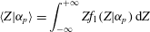 $$\begin{eqnarray}\langle Z|{\it\alpha}_{p}\rangle =\int _{-\infty }^{+\infty }Zf_{1}(Z|{\it\alpha}_{p})\,\text{d}Z\end{eqnarray}$$
and is related to the PA statistic by
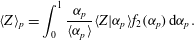 $$\begin{eqnarray}\langle Z\rangle _{p}=\int _{0}^{1}\frac{{\it\alpha}_{p}}{\langle {\it\alpha}_{p}\rangle }\langle Z|{\it\alpha}_{p}\rangle f_{2}({\it\alpha}_{p})\,\text{d}{\it\alpha}_{p}.\end{eqnarray}$$
For CIT, some prime candidates for conditioning are (i) the vertical fluid velocity component
 $u_{f,1}$
, which appears in the drag production term, (ii) the vertical velocity difference
 $u_{p,1}-u_{f,1}$
, which appears in the mean momentum drag exchange term, and (iii) the components of the particle-phase fluctuation energy
 $k_{p}$
and
 ${\it\Theta}$
. (Recall that
 $\langle u_{f,1}\rangle _{f}=0$
and hence
 $\langle u_{f,1}\mid {\it\alpha}_{p}\rangle$
is equivalent to the conditional expected value of the drift velocity introduced in appendix A.)
In figure 17,
 $\langle u_{f,1}\mid {\it\alpha}_{p}\rangle /\mathscr{V}$
is plotted versus
 ${\it\alpha}_{p}/\langle {\it\alpha}_{p}\rangle$
for the three
 $\mathit{Re}_{p}$
. As was observed in figure 10, for small
 ${\it\alpha}_{p}$
the conditional drift velocity is positive and for large
 ${\it\alpha}_{p}$
it is negative, corresponding to stronger fluid entrainment by larger clusters. However, we can also note that the dependence on
 ${\it\alpha}_{p}$
decreases with increasing
 $\mathit{Re}_{p}$
, so that, presumably, for large enough
 $\mathit{Re}_{p}$
the drift velocity would become independent of
 ${\it\alpha}_{p}$
. As noted in table 2, the fraction of the kinetic energy production that goes to turbulent kinetic energy (i.e.
 $\text{DP}/({\it\varphi}\langle u_{p,1}\rangle _{p}g)$
) decreases with increasing
 $\mathit{Re}_{p}$
. Because the drift velocity determines DP, the fact that the conditional drift velocity becomes flatter for increasing
 $\mathit{Re}_{p}$
explains why
 $\text{DP}/({\it\varphi}\langle u_{p,1}\rangle _{p}g)$
decreases. Physically, the decorrelation of drift velocity with
 ${\it\alpha}_{p}$
is probably due to the less effective transfer of momentum from the particles to the fluid as
 $\mathit{Re}_{p}$
increases. Because our simulations are done with a constant
 ${\it\tau}_{p}$
(i.e. there is no explicit dependence on
 $\mathit{Re}_{p}$
), one possible explanation would be that turbulent kinetic energy is dissipated locally in fully resolved wakes and boundary layers around the particles, and therefore it is not effective in producing the large-scale fluid turbulence seen in CIT. Experimental measurements by Aliseda et al. (Reference Aliseda, Cartellier, Hainaux and Lasheras2002) of heavy particles in decaying homogeneous isotropic turbulence suggested that clusters act as large pseudo-particles that add to the settling velocity of the particles inside them. Indeed, if clusters are approximated as pseudo-particles with length scale proportional to
 ${\it\alpha}^{1/3}$
, then the effective cluster Reynolds number will scale like
 $\mathit{Re}_{c}\approx \mathit{Re}_{p}(1+{\it\beta}{\it\alpha}_{p}^{1/3})$
, where
 ${\it\beta}$
is a scaling parameter. With this scaling, large clusters will have a significantly larger
 $\mathit{Re}_{c}$
, implying that they will generate significant fluid-phase vorticity in their wakes and boundary layers. Note that this interpretation is consistent with figure 17, where we observe that the curves flatten out faster for large
 ${\it\alpha}_{p}$
. In any case, based on the results in figure 17, it is clear that, in order to accurately model the drag production term DP, it will be necessary to account for loss of turbulent kinetic energy production with increasing cluster size.
Turning now to the normalized conditional slip velocity shown in figure 18, we observe that the three curves exhibit good collapse. Recall from § 4.4 that the unconditional slip velocity
 $|\langle u_{p,1}\rangle _{p}-\langle u_{f,1}\rangle _{p}|$
is very close to
 $\mathscr{V}$
. Thus, the result in figure 18 implies that
 $$\begin{eqnarray}\langle u_{p,1}|{\it\alpha}_{p}\rangle =\langle u_{f,1}|{\it\alpha}_{p}\rangle -\mathscr{V}h({\it\alpha}_{p}/\langle {\it\alpha}_{p}\rangle ),\end{eqnarray}$$
where the function
 $h>0$
with the property
 $\langle h\rangle _{p}=1$
is the collapsed curve in figure 18. For example, a simple function that produces the correct asymptotic behaviour for large
 ${\it\alpha}_{p}$
is
 $h(x)=0.35+0.65/x$
. Note that, because
 $\mathscr{V}={\it\tau}_{p}g$
, we can interpret
 $h(x)$
to be a cluster-size-dependent correction to the drag time scale, i.e.
 ${\it\tau}_{c}={\it\tau}_{p}h({\it\alpha}_{p}/\langle {\it\alpha}_{p}\rangle )$
is the effective cluster drag time scale in CIT.
Slip velocity conditioned on
 ${\it\alpha}_{p}$
from single realizations of fully developed CIT with
 $\mathit{Re}_{p}=0.25$
(——),
 $\mathit{Re}_{p}=0.5$
(– – –),
 $\mathit{Re}_{p}=1$
(
 $\cdots \cdots$
) and
 $h(x)=0.35+0.65/x$
(○).
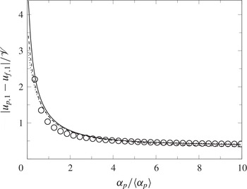
In figure 19 the normalized conditional granular energy components are plotted versus
 ${\it\alpha}_{p}$
. First, note that the uncorrelated granular temperature represents a relatively small fraction of the total conditional granular energy. For the correlated component, it is clear from the curves for conditional
 $k_{p}$
that no collapse is observed for CIT. In fact, the behaviour for small
 ${\it\alpha}_{p}$
is quite different over the range of
 $\mathit{Re}_{p}$
investigated. From these observations, we can conclude that conditioning the particle turbulent kinetic energy on
 ${\it\alpha}_{p}$
is unlikely to simplify the modelling effort. In comparison, the conditional granular temperature curves in figure 19 show somewhat better collapse. Because the granular temperature is needed to estimate the particle–particle collision rate, it may be worthwhile to attempt to model the conditional granular temperature. However, in CIT we observed that energy dissipation due to inelastic collisions plays a minor role in the overall kinetic energy balance. Thus, given the relatively weak dependence of
 $\langle {\it\Theta}|{\it\alpha}_{p}\rangle$
on
 ${\it\alpha}_{p}$
in figure 19, using the unconditional mean
 $\langle {\it\Theta}\rangle _{p}$
may suffice for CIT.
Components of the fluctuating granular energy conditioned on
 ${\it\alpha}_{p}$
from single realizations of fully developed CIT. PA particle-phase kinetic energy
 $k_{p}$
from
 $\mathit{Re}_{p}=0.25$
(——),
 $\mathit{Re}_{p}=0.5$
(– – –) and
 $\mathit{Re}_{p}=1$
(
 $\boldsymbol{\cdots }\!\!$
). Granular temperature
 ${\it\Theta}$
from
 $\mathit{Re}_{p}=0.25$
(——),
 $\mathit{Re}_{p}=0.5$
(– – –) and
 $\mathit{Re}_{p}=1$
(
 $\cdots \cdots$
).
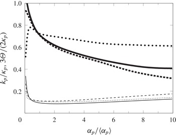
Finally, it is noteworthy that the instantaneous granular temperature dynamics shown in figure 2 do not have a significant effect on
 $\langle {\it\Theta}|{\it\alpha}_{p}\rangle$
. On closer inspection, the reason for this behaviour is that the value of
 ${\it\alpha}_{p}$
is not strongly correlated with regions of strong compression (i.e.
 $-\boldsymbol{{\rm\nabla}}\boldsymbol{\cdot }\boldsymbol{u}_{p}\gg 0$
). For example, the zoomed-in snapshot in figure 2 is a region where
 ${\it\alpha}_{p}$
changes rapidly and compression is strong. However, on the back side of the same cluster the same range of
 ${\it\alpha}_{p}$
is observed, but with expansion instead of compression. Overall, the two regions average out for the same value of
 ${\it\alpha}_{p}$
, leaving no net effect on
 $\langle {\it\Theta}|{\it\alpha}_{p}\rangle$
.
4.6. Two-point statistics
As already shown in § 3.4.2, two-point statistics contain detailed information of the spatial structure inherent to the turbulent flow field. Along with the two-point particle correlations defined in § 3.4.2, the two-point PA fluid velocity correlation can be expressed as
 $$\begin{eqnarray}\widetilde{R}_{ij}^{f}(\boldsymbol{r})=\frac{\langle {\it\alpha}_{f}(\boldsymbol{x},t){\it\alpha}_{f}(\boldsymbol{x}+\boldsymbol{r},t)u_{f,i}^{\prime \prime \prime }(\boldsymbol{x},t)u_{f,j}^{\prime \prime \prime }(\boldsymbol{x}+\boldsymbol{r},t)\rangle }{\langle {\it\alpha}_{f}(\boldsymbol{x},t){\it\alpha}_{f}(\boldsymbol{x}+\boldsymbol{r},t)\rangle }.\end{eqnarray}$$
From this it is possible to define the vertical and spanwise fluid-phase integral length scales as
 $$\begin{eqnarray}L_{11,\Vert }^{f}\equiv \frac{1}{\widetilde{R}_{11}^{f}(0)}\int _{0}^{\infty }\widetilde{R}_{11}^{f}(r_{1})\,\text{d}r_{1},\quad L_{11,\bot }^{f}\equiv \frac{1}{\widetilde{R}_{11}^{f}(0)}\int _{0}^{\infty }\widetilde{R}_{11}^{f}(r_{2})\,\text{d}r_{2}\end{eqnarray}$$
and
 $$\begin{eqnarray}L_{22,\Vert }^{f}\equiv \frac{1}{\widetilde{R}_{22}^{f}(0)}\int _{0}^{\infty }\widetilde{R}_{22}^{\,f}(r_{1})\,\text{d}r_{1},\quad L_{22,\bot }^{f}\equiv \frac{1}{\widetilde{R}_{22}^{f}(0)}\int _{0}^{\infty }\widetilde{R}_{22}^{f}(r_{2})\,\text{d}r_{2},\end{eqnarray}$$
where the subscript
 $\Vert$
denotes a pair separation (
 $r_{1}$
) measured in the vertical direction and
 $\bot$
denotes a pair separation (
 $r_{2}$
) measured in the horizontal direction. Note that, owing to the statistical homogeneity of the flows considered in this work, the integral length scales are not a function of space or time. Similarly, particle integral length scales can be defined as
 $$\begin{eqnarray}L_{11,\Vert }^{p}\equiv \frac{1}{R_{11}^{p}(0)}\int _{0}^{\infty }R_{11}^{p}(r_{1})\,\text{d}r_{1},\quad L_{11,\bot }^{p}\equiv \frac{1}{R_{11}^{p}(0)}\int _{0}^{\infty }R_{11}^{p}(r_{2})\,\text{d}r_{2}\end{eqnarray}$$
and
 $$\begin{eqnarray}L_{22,\Vert }^{p}\equiv \frac{1}{R_{22}^{p}(0)}\int _{0}^{\infty }R_{22}^{p}(r_{1})\,\text{d}r_{1},\quad L_{22,\bot }^{p}\equiv \frac{1}{R_{22}^{p}(0)}\int _{0}^{\infty }R_{22}^{p}(r_{2})\,\text{d}r_{2}.\end{eqnarray}$$
Here we have defined the particle-phase integral length scales using the Lagrangian two-point correlations, as they do not depend on the accuracy of the filter and represent the exact spatial distribution of the particles. Another integral length scale of interest can be computed from the RDF in order to define a characteristic cluster size, given by
 $$\begin{eqnarray}L_{\Vert }^{{\it\alpha}}\equiv \frac{1}{g_{0}(0)-1}\int _{0}^{\infty }[g_{0}(r_{1})-1]\,\text{d}r_{1}\quad \text{and}\quad L_{\bot }^{{\it\alpha}}\equiv \frac{1}{g_{0}(0)-1}\int _{0}^{\infty }[g_{0}(r_{2})-1]\,\text{d}r_{2}.\end{eqnarray}$$
The integral length scales computed from the two-point velocity correlations can be used to define the following integral time scales for the fluid phase,
 $$\begin{eqnarray}T_{11,\Vert }^{f}\equiv \frac{L_{11,\Vert }^{f}}{\langle u_{f,1}^{\prime \prime \prime 2}\rangle _{f}^{1/2}},\quad T_{11,\bot }^{f}\equiv \frac{L_{11,\bot }^{f}}{\langle u_{f,1}^{\prime \prime \prime 2}\rangle _{f}^{1/2}},\end{eqnarray}$$
 $$\begin{eqnarray}T_{22,\Vert }^{f}\equiv \frac{L_{22,\Vert }^{f}}{\langle u_{f,2}^{\prime \prime \prime 2}\rangle _{f}^{1/2}},\quad T_{22,\bot }^{f}\equiv \frac{L_{22,\bot }^{f}}{\langle u_{f,2}^{\prime \prime \prime 2}\rangle _{f}^{1/2}},\end{eqnarray}$$
and for the particle phase,
 $$\begin{eqnarray}T_{11,\Vert }^{p}\equiv \frac{L_{11,\Vert }^{p}}{\langle u_{p,1}^{\prime \prime 2}\rangle _{p}^{1/2}},\quad T_{11,\bot }^{p}\equiv \frac{L_{11,\bot }^{p}}{\langle u_{p,1}^{\prime \prime 2}\rangle _{p}^{1/2}},\end{eqnarray}$$
 $$\begin{eqnarray}T_{22,\Vert }^{p}\equiv \frac{L_{22,\Vert }^{p}}{\langle u_{p,2}^{\prime \prime 2}\rangle _{p}^{1/2}},\quad T_{22,\bot }^{p}\equiv \frac{L_{22,\bot }^{p}}{\langle u_{p,2}^{\prime \prime 2}\rangle _{p}^{1/2}}.\end{eqnarray}$$
The integral length and time scales for the fluid and particle phases are reported in tables 12 and 13, respectively.
Integral length and time scales associated with the fluid phase.
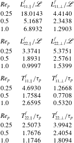
Integral length and time scales associated with the particle phase.
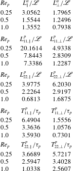
Over the range of
 $\mathit{Re}_{p}$
considered, we observe that, in general, the integral length scales normalized by
 $\mathscr{L}$
decrease with increasing
 $\mathit{Re}_{p}$
. The same trend is observed for the integral time scales. Results for larger
 $\mathit{Re}_{p}$
would be needed to determine whether these length and time scales become independent of
 $\mathit{Re}_{f}$
in the high-Reynolds-number limit. In figures 20–22 the radial distribution functions and two-point velocity correlations are plotted using the corresponding integral length scale to normalize the separation distance. For the radial distribution functions in figure 20, an excellent collapse of the curves is found for all
 $\mathit{Re}_{p}$
. For the two-point velocity correlations in figures 21 and 22, the collapse is not as good, but still reasonable. Moreover, note that the velocity correlations exhibit good decay, confirming that the periodic domain used in our simulations is large enough to avoid finite-domain-size effects. Based on preliminary simulations on smaller domains, we find that, when the periodic domain is too small, particles tend to cluster in vertical columns, which has a strong negative effect on the accuracy of the one-point turbulence statistics. For example, the magnitude of the fluid velocity
 $\langle u_{f,1}\rangle _{p}$
is significantly underpredicted on smaller domains.
Radial distribution functions from single realizations of the fully developed CIT computed in the (a) streamwise and (b) spanwise directions.
 $\mathit{Re}_{p}=0.25$
(——),
 $\mathit{Re}_{p}=0.5$
(– – –) and
 $\mathit{Re}_{p}=1$
(
 $\cdots \cdots$
).
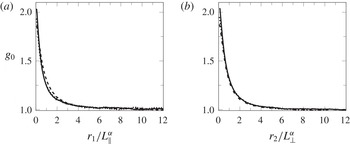
Two-point particle velocity correlations from single realizations of the fully developed CIT simulations.
 $\mathit{Re}_{p}=0.25$
(——),
 $\mathit{Re}_{p}=0.5$
(– – –) and
 $\mathit{Re}_{p}=1$
(
 $\cdots \cdots$
).
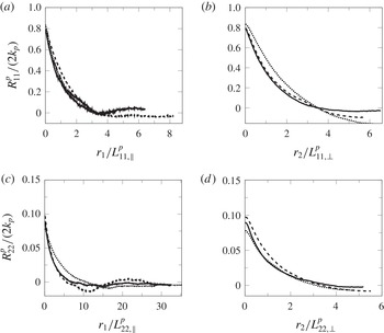
Two-point fluid velocity correlations from single realizations of the fully developed CIT simulations.
 $\mathit{Re}_{p}=0.25$
(——),
 $\mathit{Re}_{p}=0.5$
(– – –) and
 $\mathit{Re}_{p}=1$
(
 $\cdots \cdots$
).
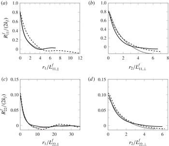
Finally, note that the integral length scales from the radial distribution functions are smaller than those for the fluid velocity correlations. Given that the fluid-phase turbulence is generated by momentum coupling with the clusters in the particle phase, the larger integral length scales in the fluid phase provide a mechanism for breaking up particle clusters on smaller scales, thereby sustaining the nearly lognormal p.d.f. shown in figure 13. On the contrary, if the fluid integral length scales were smaller than the average cluster size (e.g. due to pseudo-turbulence generated by individual particles), then clusters would probably continue to grow to the length scale of the periodic domain (which is observed when the simulation domain is too small). In addition, it can be seen that the length scale
 $\mathscr{L}$
yields a reasonable prediction for the characteristic cluster size (
 $L_{\Vert }^{{\it\alpha}}$
and
 $L_{\bot }^{{\it\alpha}}$
), but, owing to the formation of wakes, this length scale severely underpredicts the velocity length scales of each phase. Nonetheless, the exact mechanism that determines the integral length scales of the clusters and their one-point p.d.f. has yet to be elucidated, and thus the scaling behaviour of CIT as a function of
 $\mathit{Re}_{f}$
remains an open question.
5. Summary and conclusions
The present study investigates the turbulence characteristics in strongly coupled fluid–particle flows to better understand the key physical mechanisms required in developing a predictive macroscopic turbulence model. To isolate the effects of momentum coupling between the phases, this work considers fully developed cluster-induced turbulence (CIT) under a range of particle Reynolds numbers. In statistically homogeneous suspensions with significant mass loading, particles self-organize into dense clusters and generate volume-fraction and velocity fluctuations that produce and sustain fluid turbulence even in the absence of mean shear. Because the density ratio of the two phases is very large in gas–particle flows, CIT is ubiquitous in practical engineering and environmental flows when body forces or inlet conditions generate a mean velocity difference, such as the gravity-driven flows considered herein. Surprisingly, despite its importance, very little is known about the fundamental properties of CIT. To this end, a complete description of the two-phase flow was presented in terms of the exact Reynolds-average (RA) equations, and the relevant unclosed terms that are retained in the context of homogeneous gravity-driven flows were investigated numerically.
Simulations of gravity-driven CIT with mean mass loading
 ${\it\varphi}=10$
and particle Reynolds numbers
 $\mathit{Re}_{p}=0.25$
, 0.5 and 1 were conducted via an Eulerian–Lagrangian framework. Special care was taken during interphase exchange processes to decouple the ratio of particle diameter to mesh size. An adaptive filtering technique recently introduced in our previous work (Capecelatro et al.
Reference Capecelatro, Desjardins and Fox2014a
) was used to evaluate the Lagrangian data as Eulerian fields that are consistent with the terms appearing in the RA equations. The filtering approach samples the particles with an averaging volume that adapts to the local flow field, allowing for a sufficient number of particles to be sampled in dilute regions of the flow, while remaining optimally compact in dense clusters. To assess the accuracy of the filter, velocity correlations and radial distribution functions computed from the filtered Eulerian fields were compared to Lagrangian two-point statistics. It was shown that the filter is capable of capturing the spatial distribution of particle position and velocity with minimal error for the range of Reynolds numbers considered.
In formulating the RA equations, the instantaneous particle velocity was decomposed into a continuous (filtered) velocity field and a spatially uncorrelated (residual) contribution. With this, the total particle fluctuation energy
 ${\it\kappa}_{p}$
was expressed as the sum of the phase-average (PA) turbulent kinetic energy
 $k_{p}$
and PA granular temperature
 $\langle {\it\Theta}\rangle _{p}$
. Observations from the simulations indicate that high values of the granular temperature correspond to regions in front of falling clusters where the correlated component of the particle-phase velocity is strongly compressed in the vertical direction, referred to as compressive heating. Along with compressive heating of the particle phase, viscous dissipation of mean kinetic energy represents dissipation of
 $k_{p}$
that enters as production terms in the transport of
 $\langle {\it\Theta}\rangle _{p}$
. In addition, particles were observed to accumulate in regions of low vorticity, resembling preferential concentration that typically occurs in dilute particle-laden turbulence. However, in CIT the vorticity is generated in shear layers between clusters, unlike in classical preferential concentration, where vorticity would exist even in the absence of the disperse phase.
One-point statistics were computed for the principal quantities of interest for both the fluid and particle phases. From these statistics, it was shown that the momentum coupling between the two phases leads to significant differences from the behaviour observed in very dilute systems with one-way coupling. In particular, entrainment of the fluid in dense regions of the flow results in an increased mean particle velocity that generates a drag production term for fluid-phase turbulent kinetic energy that is highly anisotropic. Owing to the compressibility of the particle phase, the uncorrelated components of the particle-phase velocity statistics are highly non-Gaussian, as opposed to systems with one-way coupling, where, in the homogeneous limit, all of the velocity statistics are nearly Gaussian (Minier & Peirano Reference Minier and Peirano2001). These differences would suggest that a predictive p.d.f. model for CIT must explicitly account for the compressibility of the particle phase. Moreover, it is typically assumed that the particle-phase Knudsen number is very small, so that a Chapman–Enskog expansion can be used to provide constitutive relations for the particle pressure tensor (Lun et al. Reference Lun, Savage, Jeffrey and Chepuriny1984). In this study, we find that the uncorrelated particle velocity statistics are significantly anisotropic, and transport equations for the separate components of the pressure tensor are necessary for predicting fully developed CIT.
A detailed analysis of the one-point statistics provided insight on the overall kinetic energy balance for CIT. It was found that particles falling under the influence of gravity generate mean kinetic energy, which, in the absence of clustering, is balanced by mean drag and eventually leads to viscous heating of the fluid. Owing to the formation of clusters, in fully developed CIT the average falling velocity of particles increases significantly relative to the terminal velocity for an isolated particle under similar conditions, with an increasing effect at lower Reynolds numbers. Some of this additional particle-phase kinetic energy is transferred to fluid-phase turbulent kinetic energy through drag production, which is dissipated to heat the fluid by viscous dissipation. In the fluid phase, dissipation of turbulent kinetic energy results from resolved small-scale velocity fluctuations that are common to single-phase turbulence, as well as drag exchange terms. The drag exchange terms have contributions from viscous dissipation of unresolved fluid velocity fluctuations, e.g. in the viscous boundary layers around individual particles, and energy transferred to the particles at the fluid–particle interface. We observe that the relative contribution of the interphase energy exchange is approximately 22 % for all Reynolds numbers, while nearly 80 % of the turbulent kinetic energy is dissipated by unresolved viscous dissipation. Interestingly, the fraction of the total kinetic energy production going to drag production increases with decreasing Reynolds number. It is hypothesized that in fully developed flows all of the kinetic energy produced in the system will lead to drag production as the particle Reynolds number approaches zero.
In fully developed CIT, the particle-phase volume fraction has a one-point p.d.f. close to lognormal that exhibits large fluctuations about its mean value. As a first step in developing models for predicting the volume-fraction variance, one-point statistics conditioned on the local volume fraction were investigated. Because the mean value of the vertical fluid velocity component is null, its instantaneous value conditioned on the particle-phase volume fraction is equivalent to the conditional expected value of the drift that appears in the drag production term. It was observed that, for small values of particle-phase volume fraction, the conditional drift velocity is positive, and for large values it is negative, corresponding to stronger fluid entrainment by larger clusters. This dependence on volume fraction was seen to decrease with increasing particle Reynolds number, suggesting that the drift velocity would become independent of volume fraction at large enough Reynolds numbers. As previously noted, the fraction of the kinetic energy production that goes to turbulent kinetic energy decreases with increasing Reynolds number. Because the drift velocity determines drag production, the fact that the conditional drift velocity becomes flatter for increasing Reynolds number explains why the fraction of kinetic energy production decreases.
Concerning the components of granular energy conditioned on the particle-phase volume fraction, it was found that the conditional granular temperature represents only a relatively small fraction of the total energy. Because local regions of high particle volume fraction exhibit both expansion and compression of the particle velocity field, the granular temperature (which is produced in regions of high compression) was found to be uncorrelated with volume fraction. For the correlated component of granular energy, it was clear from the curves of conditional
 $k_{p}$
that no collapse is observed for CIT. In fact, the behaviour for small particle-phase volume fraction is quite different over the range of particle Reynolds numbers investigated. From these observations, we can conclude that conditioning the particle-phase turbulent kinetic energy on the volume fraction is unlikely to simplify the modelling effort. In comparison, the conditional granular temperature curves exhibited somewhat better collapse, but, given its relatively weak dependence on the particle-phase volume fraction, using the unconditional mean granular temperature may suffice when modelling CIT.
Although this work presents many new insights on the turbulence characteristics of coupled fluid–particle flows, significant future research efforts are needed to fully understand the various mechanisms that control CIT. The wide range of spatial and temporal scales associated with fully developed CIT remains a key challenge. It was shown that the length scale
 $\mathscr{L}={\it\tau}_{p}^{2}g$
yields a reasonable prediction for the characteristic cluster size, but severely underpredicts the velocity length scales of each phase due to the formation of wakes past clusters. It is recommended in future studies of gravity-induced (i.e. settling) fluid–particle flows that careful attention is paid to assessing the size of the computational domain. In particular, the domain size in the mean-flow direction should be significantly larger than
 $\mathscr{L}$
. In this work, two-point velocity correlations were observed to exhibit good decay, confirming that the periodic domain was large enough to avoid finite-domain-size effects. If the domain size is too small, we expect the multiphase statistics to be severely compromised. For example, integral length scales computed from the radial distribution functions were found to be smaller than those for the fluid velocity correlations. Given that the fluid-phase turbulence is generated by momentum coupling with the clusters in the particle phase, the larger integral length scales in the fluid phase provide a mechanism for breaking up particle clusters on smaller scales, thereby sustaining the nearly lognormal p.d.f. of volume fraction observed. If the fluid integral length scales were smaller than the average cluster size, clusters would probably continue to grow to the length scale of the periodic domain (which is observed when the simulation domain is too small.) Nonetheless, the exact mechanism that determines the integral length scales of the clusters and their one-point p.d.f. has yet to be elucidated, and thus the scaling behaviour of CIT as a function of Reynolds number remains an open question.
Acknowledgements
Part of the research leading to the results reported in this work has received funding from the European Union Seventh Framework Programme (FP7/2007–2013) under agreement no. 246556. The research reported in this paper is partially supported by the HPC equipment purchased through US National Science Foundation MRI grant no. CNS 1229081 and CRI grant no. 1205413.
Appendix A. Statistics for the fluid phase seen by the particles
Statistical quantities for the fluid seen by the particles arise naturally in the phase-coupling terms in gas–particle flows. By definition, such quantities represent fluid-phase properties weighted by the presence of the particle phase. In the RA equations, they appear in the form
 $\langle {\it\alpha}_{p}A\rangle$
, where
 $A$
is a fluid-phase field such as the fluid velocity. For example,
 $\langle {\it\alpha}_{p}\boldsymbol{u}_{f}\rangle =\langle {\it\alpha}_{p}\rangle \langle \boldsymbol{u}_{f}\rangle _{p}$
defines the mean fluid velocity seen by the particles denoted by
 $\langle \boldsymbol{u}_{f}\rangle _{p}$
. It is, therefore, of interest to derive the transport equations for such statistics in order to compare them, for example, to stochastic models for the fluid seen by the particles (see e.g. Minier & Peirano Reference Minier and Peirano2001).
A.1. Transport equation for fluid statistics seen by the particles
The transport equation for any fluid quantity of interest can be derived starting from the mesoscale model equations in § 2.2. Given the equality
 $$\begin{eqnarray}\langle {\it\alpha}_{p}A\rangle =\langle A\rangle -\langle {\it\alpha}_{f}\rangle \langle A\rangle _{f},\end{eqnarray}$$
we observe that a simple method for deriving the equation for
 $\langle {\it\alpha}_{p}A\rangle$
is to take the RA of the equation for
 $A$
and to subtract from it the PA fluid-phase equation derived in § 2.4.2. For example, doing this for the fluid velocity (2.10) leads to
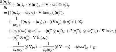 $$\begin{eqnarray}\displaystyle & & \displaystyle \frac{\partial \langle \boldsymbol{u}_{f}\rangle _{p}}{\partial t}+\langle \boldsymbol{u}_{f}\rangle _{p}\boldsymbol{\cdot }\boldsymbol{{\rm\nabla}}\langle \boldsymbol{u}_{f}\rangle _{p}+\boldsymbol{{\rm\nabla}}\boldsymbol{\cdot }\langle \boldsymbol{u}_{f}^{\prime \prime }\otimes \boldsymbol{u}_{f}^{\prime \prime }\rangle _{p}\nonumber\\ \displaystyle & & \displaystyle \quad =[(\langle \boldsymbol{u}_{p}\rangle _{p}-\langle \boldsymbol{u}_{f}\rangle _{p})\boldsymbol{\cdot }\boldsymbol{{\rm\nabla}}\ln \langle {\it\alpha}_{p}\rangle ]\langle \boldsymbol{u}_{f}^{\prime \prime \prime }\rangle _{p}\nonumber\\ \displaystyle & & \displaystyle \qquad +\,\frac{1}{\langle {\it\alpha}_{p}\rangle }(\langle \boldsymbol{u}_{f}\rangle _{p}-\langle \boldsymbol{u}_{p}\rangle _{p})\boldsymbol{\cdot }\langle (\boldsymbol{{\rm\nabla}}{\it\alpha}_{p}^{\prime })\otimes \boldsymbol{u}_{f}^{\prime \prime \prime }\rangle +\mathscr{C}_{p}\nonumber\\ \displaystyle & & \displaystyle \qquad +\,\langle {\it\alpha}_{f}\rangle (\langle \boldsymbol{u}_{f}^{\prime \prime \prime }\otimes \boldsymbol{u}_{f}^{\prime \prime \prime }\rangle _{f}-\langle \boldsymbol{u}_{f}^{\prime \prime \prime }\otimes \boldsymbol{u}_{f}^{\prime \prime \prime }\rangle _{p}+2\langle \boldsymbol{u}_{f}^{\prime \prime \prime }\rangle _{p}\otimes \langle \boldsymbol{u}_{f}^{\prime \prime \prime }\rangle _{p})\boldsymbol{\cdot }\boldsymbol{{\rm\nabla}}\ln \langle {\it\alpha}_{p}\rangle \nonumber\\ \displaystyle & & \displaystyle \qquad -\,\langle \boldsymbol{u}_{f}^{\prime \prime \prime }\otimes \boldsymbol{u}_{p}^{\prime \prime }\rangle \boldsymbol{\cdot }\boldsymbol{{\rm\nabla}}\ln \langle {\it\alpha}_{p}\rangle \nonumber\\ \displaystyle & & \displaystyle \qquad -\,\frac{1}{{\it\rho}_{p}\langle {\it\alpha}_{p}\rangle }\langle {\it\phi}\boldsymbol{{\rm\nabla}}p_{f}\rangle +\frac{1}{{\it\rho}_{p}\langle {\it\alpha}_{p}\rangle }\langle {\it\phi}\boldsymbol{{\rm\nabla}}\boldsymbol{\cdot }{\bf\sigma}_{f}\rangle -\langle {\it\phi}\mathbf{\mathscr{A}}\rangle _{p}+\boldsymbol{g},\end{eqnarray}$$
where
 $\langle \boldsymbol{u}_{f}^{\prime \prime \prime }\rangle _{p}=\langle \boldsymbol{u}_{f}\rangle _{p}-\langle \boldsymbol{u}_{f}\rangle _{f}$
. The RA cross-correlation term in the fifth line of (A 2) can be further expanded in terms of the phase averages:
 $$\begin{eqnarray}\langle \boldsymbol{u}_{f}^{\prime \prime }\otimes \boldsymbol{u}_{p}^{\prime \prime }\rangle =\langle {\it\alpha}_{f}\rangle \langle \boldsymbol{u}_{f}^{\prime \prime }\otimes \boldsymbol{u}_{p}^{\prime \prime }\rangle _{f}+\langle {\it\alpha}_{p}\rangle \langle \boldsymbol{u}_{f}^{\prime \prime \prime }\otimes \boldsymbol{u}_{p}^{\prime \prime }\rangle _{p}.\end{eqnarray}$$
The term
 $\mathscr{C}_{p}$
is unclosed and defined by
 $$\begin{eqnarray}\mathscr{C}_{p}=\langle \boldsymbol{u}_{f}^{\prime \prime }\boldsymbol{{\rm\nabla}}\boldsymbol{\cdot }(\boldsymbol{u}_{f}^{\prime \prime \prime }-\boldsymbol{u}_{p}^{\prime \prime })\rangle _{p}+\frac{1}{\langle {\it\alpha}_{p}\rangle }\langle \boldsymbol{u}_{f}^{\prime \prime }\otimes (\boldsymbol{u}_{f}^{\prime \prime }-\boldsymbol{u}_{p}^{\prime \prime })\boldsymbol{\cdot }\boldsymbol{{\rm\nabla}}{\it\alpha}_{p}^{\prime }\rangle _{p}.\end{eqnarray}$$
In these equations, the fluctuation with respect to the particle PA is denoted by
 $A^{\prime \prime }=A-\langle A\rangle _{p}$
. Note that (A 2) can be written in several equivalent forms by using the two identities
 ${\it\alpha}_{p}+{\it\alpha}_{f}=1$
and
 $\boldsymbol{{\rm\nabla}}\boldsymbol{\cdot }({\it\alpha}_{p}\boldsymbol{u}_{p}+{\it\alpha}_{f}\boldsymbol{u}_{f})=0$
. The same methodology can be applied to find the transport equation for higher-order statistics such as the fluid-phase Reynolds stresses seen by the particle
 $\langle \boldsymbol{u}_{f}^{\prime \prime }\otimes \boldsymbol{u}_{f}^{\prime \prime }\rangle _{p}$
. It is interesting to note that (A 2) depends on the particle-phase volume fraction
 ${\it\alpha}_{p}$
, even in the very dilute limit (i.e.
 ${\it\varphi}\ll 1$
, one-way coupling) where the momentum exchange terms are negligible. The dependence on the fluctuations of the particle-phase volume fraction (e.g. preferential concentration) is neglected in Lagrangian p.d.f. methods for dilute gas–particle flows (see, e.g. Minier & Peirano Reference Minier and Peirano2001).
While it is exact, (A 2) contains new unclosed terms, one of the most important of which is the drag coupling,
 $$\begin{eqnarray}\frac{1}{{\it\tau}_{p}}(\langle {\it\phi}\boldsymbol{u}_{p}\rangle _{p}-\langle {\it\phi}\boldsymbol{u}_{f}\rangle _{p})=\frac{{\it\rho}_{p}}{{\it\rho}_{f}{\it\tau}_{p}}(\langle \boldsymbol{u}_{p}\rangle _{p}-\langle \boldsymbol{u}_{f}\rangle _{p})+\frac{1}{{\it\tau}_{p}}\langle {\it\phi}^{\prime }(\boldsymbol{u}_{p}-\boldsymbol{u}_{f})\rangle _{p},\end{eqnarray}$$
where
 ${\it\phi}^{\prime }={\it\phi}-{\it\varphi}$
is the mass-loading fluctuation. Inside clusters
 ${\it\phi}^{\prime }>0$
, and in dilute regions of the flow
 ${\it\phi}^{\prime }<0$
. From this equation, we observe that the drag term for the mean fluid velocity seen by the particles is not closed in terms of the difference in the mean velocities (
 $\langle \boldsymbol{u}_{p}\rangle _{p}-\langle \boldsymbol{u}_{f}\rangle _{p}$
). Thus, additional modelling will be required to close the final term on the right-hand side of (A 5).
Another important quantity in gas–particle flows is the drift velocity, defined by
 $\boldsymbol{u}_{d}=\langle \boldsymbol{u}_{f}^{\prime \prime \prime }\rangle _{p}$
, which modifies the particle-phase terminal velocity in (2.24) and appears in the drag production term in (2.36). The exact transport equation for the drift velocity is given by
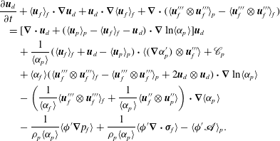 $$\begin{eqnarray}\displaystyle & & \displaystyle \frac{\partial \boldsymbol{u}_{d}}{\partial t}+\langle \boldsymbol{u}_{f}\rangle _{f}\boldsymbol{\cdot }\boldsymbol{{\rm\nabla}}\boldsymbol{u}_{d}+\boldsymbol{u}_{d}\boldsymbol{\cdot }\boldsymbol{{\rm\nabla}}\langle \boldsymbol{u}_{f}\rangle _{f}+\boldsymbol{{\rm\nabla}}\boldsymbol{\cdot }(\langle \boldsymbol{u}_{f}^{\prime \prime \prime }\otimes \boldsymbol{u}_{f}^{\prime \prime \prime }\rangle _{p}-\langle \boldsymbol{u}_{f}^{\prime \prime \prime }\otimes \boldsymbol{u}_{f}^{\prime \prime \prime }\rangle _{f})\nonumber\\ \displaystyle & & \displaystyle \quad =[\boldsymbol{{\rm\nabla}}\boldsymbol{\cdot }\boldsymbol{u}_{d}+(\langle \boldsymbol{u}_{p}\rangle _{p}-\langle \boldsymbol{u}_{f}\rangle _{f}-\boldsymbol{u}_{d})\boldsymbol{\cdot }\boldsymbol{{\rm\nabla}}\ln \langle {\it\alpha}_{p}\rangle ]\boldsymbol{u}_{d}\nonumber\\ \displaystyle & & \displaystyle \qquad +\,\frac{1}{\langle {\it\alpha}_{p}\rangle }(\langle \boldsymbol{u}_{f}\rangle _{f}+\boldsymbol{u}_{d}-\langle \boldsymbol{u}_{p}\rangle _{p})\boldsymbol{\cdot }\langle (\boldsymbol{{\rm\nabla}}{\it\alpha}_{p}^{\prime })\otimes \boldsymbol{u}_{f}^{\prime \prime \prime }\rangle +\mathscr{C}_{p}\nonumber\\ \displaystyle & & \displaystyle \qquad +\,\langle {\it\alpha}_{f}\rangle (\langle \boldsymbol{u}_{f}^{\prime \prime \prime }\otimes \boldsymbol{u}_{f}^{\prime \prime \prime }\rangle _{f}-\langle \boldsymbol{u}_{f}^{\prime \prime \prime }\otimes \boldsymbol{u}_{f}^{\prime \prime \prime }\rangle _{p}+2\boldsymbol{u}_{d}\otimes \boldsymbol{u}_{d})\boldsymbol{\cdot }\boldsymbol{{\rm\nabla}}\ln \langle {\it\alpha}_{p}\rangle \nonumber\\ \displaystyle & & \displaystyle \qquad -\left(\frac{1}{\langle {\it\alpha}_{f}\rangle }\langle \boldsymbol{u}_{f}^{\prime \prime \prime }\otimes \boldsymbol{u}_{f}^{\prime \prime \prime }\rangle _{f}+\frac{1}{\langle {\it\alpha}_{p}\rangle }\langle \boldsymbol{u}_{f}^{\prime \prime }\otimes \boldsymbol{u}_{p}^{\prime \prime }\rangle \right)\boldsymbol{\cdot }\boldsymbol{{\rm\nabla}}\langle {\it\alpha}_{p}\rangle \nonumber\\ \displaystyle & & \displaystyle \qquad -\,\frac{1}{{\it\rho}_{p}\langle {\it\alpha}_{p}\rangle }\langle {\it\phi}^{\prime }\boldsymbol{{\rm\nabla}}p_{f}\rangle +\frac{1}{{\it\rho}_{p}\langle {\it\alpha}_{p}\rangle }\langle {\it\phi}^{\prime }\boldsymbol{{\rm\nabla}}\boldsymbol{\cdot }{\bf\sigma}_{f}\rangle -\langle {\it\phi}^{\prime }\mathbf{\mathscr{A}}\rangle _{p}.\end{eqnarray}$$
The fifth line of (A 6) is the classical model for the dependence of the drift velocity on the gradient of the mean volume fraction. The (unclosed) terms in the third line of (A 6) are usually neglected, while the terms in the final line arise due to two-way coupling. It is interesting to note that the exact, closed terms in the first line of (A 6) are different from those found with the Lagrangian p.d.f. model proposed by Minier, Peirano & Chibbarro (Reference Minier, Peirano and Chibbarro2004).
In homogeneous flows such as the CIT investigated in this work, only the homogeneous terms in the third and last lines of (A 6) are non-zero, and of these the fluid-pressure-gradient (i.e. cluster buoyancy) and drag contributions are likely to be the most important. Remarkably, for inhomogeneous flows, many of the terms in (A 6) are closed. However, the fluid–particle Reynolds stress tensor
 $\langle \boldsymbol{u}_{f}^{\prime \prime }\otimes \boldsymbol{u}_{p}^{\prime \prime }\rangle _{p}$
and
 $\langle \boldsymbol{u}_{f}^{\prime \prime }\otimes \boldsymbol{u}_{f}^{\prime \prime }\rangle _{p}$
must be closed. Also note that, in very dilute gas–particle flows, the momentum exchange terms are negligible and, unless the flow is inhomogeneous (e.g. due to gradients in RA particle-phase volume fraction or the PA fluid-phase velocity), the drift velocity will be null if the terms in the third line of (A 6) are neglected. This observation is consistent with the fact that CIT will not arise spontaneously in systems with one-way coupling (Capecelatro et al.
Reference Capecelatro, Desjardins and Fox2014a
). Nonetheless, the terms
 $\langle (\boldsymbol{{\rm\nabla}}{\it\alpha}_{p}^{\prime })\otimes \boldsymbol{u}_{f}^{\prime \prime \prime }\rangle$
and
 $\mathscr{C}_{p}$
may be non-zero due to preferential concentration and settling of particles in such systems (Good et al.
Reference Good, Ireland, Bewley, Bodenschatz, Collins and Warhaft2014).
In summary, exact (but unclosed) transport equations for the statistics of the fluid seen by the particles can be derived starting directly from the mesoscale model equations presented in § 2.2. Because the mesoscale model is based on relatively general assumptions about the nature of the phase-coupling terms, the RA equations for the fluid seen by the particles will be valid for mass loadings ranging from zero up to reasonably large values. In fact, because these RA equations are derived using only the continuity equation for
 ${\it\alpha}_{p}$
, the principal theoretical difficulty that will arise is to get an accurate closure for
 $\boldsymbol{u}_{p}$
in very dilute and very dense flows (albeit for different physical reasons, as discussed in Fox (Reference Fox2012)). For example, for the moderately dense flows considered in this work, we observe that the particle-phase pressure tensor
 $\unicode[STIX]{x1D64B}$
is strongly anisotropic. A constitutive relation for the particle-phase viscous stress tensor
 ${\bf\sigma}_{p}$
that correctly accounts for this anisotropy will be needed to close the transport equation (2.16) for
 $\boldsymbol{u}_{p}$
.
A.2. One-point p.d.f. for fluid quantities seen by the particles
In § 4.3, we report one-point p.d.f.s of the fluid velocity components seen by the particles. These p.d.f.s are computed from the joint p.d.f. involving
 ${\it\alpha}_{p}$
and the fluid quantity
 $A$
as follows. Let
 $f(A,{\it\alpha}_{p})$
be the joint p.d.f. and
 $f_{p}(A)$
be the one-point p.d.f. of
 $A$
seen by the particles. These two p.d.f.s are related by
 $$\begin{eqnarray}f_{p}(A)=\int _{0}^{1}\frac{{\it\alpha}_{p}}{\langle {\it\alpha}_{p}\rangle }f(A,{\it\alpha}_{p})\,\text{d}{\it\alpha}_{p}.\end{eqnarray}$$
Likewise, the one-point p.d.f. of
 $A$
seen by the fluid is found from
 $$\begin{eqnarray}f_{f}(A)=\int _{0}^{1}\frac{1-{\it\alpha}_{p}}{\langle {\it\alpha}_{f}\rangle }f(A,{\it\alpha}_{p})\,\text{d}{\it\alpha}_{p},\end{eqnarray}$$
and the marginal p.d.f. that yields the RA statistics is
 $f(A)=\langle {\it\alpha}_{p}\rangle f_{p}(A)+\langle {\it\alpha}_{f}\rangle f_{f}(A)$
. Note that the joint p.d.f. can be written as a conditional p.d.f.,
 $f(A,{\it\alpha}_{p})=f_{1}(A|{\it\alpha}_{p})f_{2}({\it\alpha}_{p})$
, and hence the
 $k$
th moment of
 $A$
seen by the particles can be expressed as
 $$\begin{eqnarray}\langle A^{k}\rangle _{p}=\int _{0}^{1}\frac{{\it\alpha}_{p}}{\langle {\it\alpha}_{p}\rangle }\langle A^{k}|{\it\alpha}_{p}\rangle f_{2}({\it\alpha}_{p})\,\text{d}{\it\alpha}_{p},\end{eqnarray}$$
where
 $\langle A^{k}|{\it\alpha}_{p}\rangle$
is the conditional moment introduced in § 4.5. Finally, note that, when
 $A$
is independent of
 ${\it\alpha}_{p}$
, we have
 $f_{1}(A|{\it\alpha}_{p})=f_{1}(A)$
and thus
 $\langle A^{k}\rangle _{p}=\langle A^{k}\rangle$
as expected.
Appendix B. Logarithm of the particle-phase volume fraction
The continuity equation for the particle phase can be rewritten in terms of
 $X=\ln {\it\alpha}_{p}$
:
 $$\begin{eqnarray}\left.\frac{\text{D}X}{\text{D}t}\right|_{p}=\frac{\partial X}{\partial t}+\boldsymbol{u}_{p}\boldsymbol{\cdot }\boldsymbol{{\rm\nabla}}X=-\boldsymbol{{\rm\nabla}}\boldsymbol{\cdot }\boldsymbol{u}_{p},\end{eqnarray}$$
where the first term is the convected derivative following the particle phase. From the simulation results for CIT, we observe that
 $X$
is nearly Gaussian, which would suggest that the right-hand side of (B 1) can be approximated by an uncorrelated random process. The one-point p.d.f. of
 $\boldsymbol{{\rm\nabla}}\boldsymbol{\cdot }\boldsymbol{u}_{p}$
is shown in figure 23, and we observe that the curves exhibit good collapse for all
 $\mathit{Re}_{p}$
. Furthermore, the one-point p.d.f. has strong tails with highly non-Gaussian statistics, as can be seen in table 14.
The p.d.f. of
 $\boldsymbol{{\rm\nabla}}\boldsymbol{\cdot }\boldsymbol{u}_{p}$
from single realizations of fully developed CIT with
 $\mathit{Re}_{p}=0.25$
(——),
 $\mathit{Re}_{p}=0.5$
(– – –) and
 $\mathit{Re}_{p}=1$
(
 $\cdots \cdots$
) compared to a Gaussian distribution (▵).

In a homogeneous flow, the RA mean and variance of
 $X$
obey
 $$\begin{eqnarray}\frac{\partial \langle X\rangle }{\partial t}=\langle X^{\prime }\boldsymbol{{\rm\nabla}}\boldsymbol{\cdot }\boldsymbol{u}_{p}^{\prime \prime }\rangle\end{eqnarray}$$
and
 $$\begin{eqnarray}\frac{\partial \langle X^{\prime 2}\rangle }{\partial t}=\langle X^{\prime 2}\boldsymbol{{\rm\nabla}}\boldsymbol{\cdot }\boldsymbol{u}_{p}^{\prime \prime }\rangle -2\langle X^{\prime }\boldsymbol{{\rm\nabla}}\boldsymbol{\cdot }\boldsymbol{u}_{p}^{\prime \prime }\rangle .\end{eqnarray}$$
Note that the right-hand side of (B 2) arises due to the transport term on the left-hand side of (B 1). The relevant terms appearing in (B 2) and (B 3) from fully developed CIT are provided in table 14. There we observe that the statistics for
 $X$
are close to Gaussian with significant fluctuations around the mean (i.e.
 $X^{\prime }/\langle X\rangle \approx 20\,\%$
).
Appendix C. Model for Reynolds stresses
Based on the analysis of the turbulence budgets in § 4.4, we propose the following model for the Reynolds stresses:
 $$\begin{eqnarray}\begin{array}{@{}rclr@{}}\displaystyle \frac{1}{2}\frac{\partial \langle u_{f,1}^{\prime \prime \prime 2}\rangle _{f}}{\partial t}\ & =\ & \displaystyle \frac{2}{T_{f}}(\langle u_{f,2}^{\prime \prime \prime 2}\rangle _{f}-\langle u_{f,1}^{\prime \prime \prime 2}\rangle _{f})-\frac{1}{T_{f,1}}\langle u_{f,1}^{\prime \prime \prime 2}\rangle _{f} & \text{PS}/\text{VD}\\ \ & \ & \displaystyle +\,\frac{{\it\varphi}}{{\it\tau}_{p}}({\it\beta}_{fp,1}\langle u_{f,1}^{\prime \prime \prime 2}\rangle _{f}^{1/2}\langle u_{p,1}^{\prime \prime 2}\rangle _{p}^{1/2}-{\it\beta}_{f,1}\langle u_{f,1}^{\prime \prime \prime 2}\rangle _{f}) & \text{DE}\\ \ & \ & \displaystyle +\,\frac{{\it\varphi}}{{\it\tau}_{p}}C_{g}\langle u_{p,1}\rangle _{p}^{2}, & \text{DP}\end{array}\end{eqnarray}$$
 $$\begin{eqnarray}\begin{array}{@{}rclr@{}}\displaystyle \frac{1}{2}\frac{\partial \langle u_{f,2}^{\prime \prime \prime 2}\rangle _{f}}{\partial t}\ & =\ & \displaystyle \frac{1}{T_{f}}(\langle u_{f,1}^{\prime \prime \prime 2}\rangle _{f}-\langle u_{f,2}^{\prime \prime \prime 2}\rangle _{f})-\frac{1}{T_{f,2}}\langle u_{f,2}^{\prime \prime \prime 2}\rangle _{f} & \text{PS}/\text{VD}\\ \ & \ & +\,\displaystyle \frac{{\it\varphi}}{{\it\tau}_{p}}({\it\beta}_{fp,2}\langle u_{f,2}^{\prime \prime \prime 2}\rangle _{f}^{1/2}\langle u_{p,2}^{\prime \prime 2}\rangle _{p}^{1/2}-{\it\beta}_{f,2}\langle u_{f,2}^{\prime \prime \prime 2}\rangle _{f}), & \text{DE}\end{array}\end{eqnarray}$$
 $$\begin{eqnarray}\begin{array}{@{}rclr@{}}\displaystyle \frac{1}{2}\frac{\partial \langle u_{p,1}^{\prime \prime 2}\rangle _{p}}{\partial t}\ & =\ & \displaystyle \frac{2}{T_{p}}(\langle u_{p,2}^{\prime \prime 2}\rangle _{p}-\langle u_{p,1}^{\prime \prime 2}\rangle _{p})-\frac{1}{T_{p,1}}\langle u_{p,1}^{\prime \prime 2}\rangle _{p} & \text{PS}/\text{VD}\\ \ & \ & +\,\displaystyle \frac{1}{{\it\tau}_{p}}({\it\beta}_{fp,1}\langle u_{f,1}^{\prime \prime \prime 2}\rangle _{f}^{1/2}\langle u_{p,1}^{\prime \prime 2}\rangle _{p}^{1/2}-\langle u_{p,1}^{\prime \prime 2}\rangle _{p}) & \text{DE}\end{array}\end{eqnarray}$$
and
 $$\begin{eqnarray}\begin{array}{@{}rclr@{}}\displaystyle \frac{1}{2}\frac{\partial \langle u_{p,2}^{\prime \prime 2}\rangle _{p}}{\partial t}\ & =\ & \displaystyle \frac{1}{T_{p}}(\langle u_{p,1}^{\prime \prime 2}\rangle _{p}-\langle u_{p,2}^{\prime \prime 2}\rangle _{p})-\frac{1}{T_{p,2}}\langle u_{p,2}^{\prime \prime 2}\rangle _{p} & \text{PS}/\text{VD}\\ \ & \ & +\,\displaystyle \frac{1}{{\it\tau}_{p}}({\it\beta}_{fp,2}\langle u_{f,2}^{\prime \prime \prime 2}\rangle _{f}^{1/2}\langle u_{p,2}^{\prime \prime 2}\rangle _{p}^{1/2}-\langle u_{p,2}^{\prime \prime 2}\rangle _{p}). & \text{DE}\end{array}\end{eqnarray}$$
The time constants and correlation coefficients can be fitted to the budget terms, and the resulting values are given in table 15. PS and VD are modelled by linear return-to-isotropy and turbulent energy dissipation terms, respectively. The DE and DP terms are modelled as proposed in Fox (Reference Fox2014).
One-point statistics characterizing the logarithm of the particle-phase volume fraction
 $X$
.

Time scales and correlation coefficients for Reynolds stress model.

The coefficient
 $C_{g}$
decreases with increasing
 $\mathit{Re}_{p}$
due to the less efficient momentum coupling discussed after figure 17. It is noteworthy that, except for
 ${\it\beta}_{f,1}$
, the other correlation coefficients are very similar even though they represent different physics (i.e.
 ${\it\beta}_{f,2}$
is related to fluid velocity fluctuations seen by particles, while
 ${\it\beta}_{fp,1}$
and
 ${\it\beta}_{fp,2}$
are cross-correlations between fluid and particle velocity fluctuations). The fact that
 ${\it\beta}_{f,1}>1$
indicates that the vertical fluid velocity fluctuations seen by the particles are larger than those seen by the fluid. However, because DP is producing these fluctuations, it is not unexpected to have
 ${\it\beta}_{f,1}>1$
.
The time scales for return to isotropy (
 $T_{f}$
and
 $T_{p}$
) decrease with increasing
 $\mathit{Re}_{p}$
, but have very different values for the fluid phase compared to the particle phase. However, as seen in the main text, the anisotropy between the vertical and horizontal velocity components is nearly independent of
 $\mathit{Re}_{p}$
. Thus, it is likely that drag exchange (DE) and production (DP), which are large terms in the fluid phase (see table 8), control the degree of anisotropy. The fluid viscous dissipation time scales,
 $T_{f,1}$
and
 $T_{f,2}$
, increase with
 $\mathit{Re}_{p}$
, but again VD is small compared to DE and DP so that the values of these time scales have a small effect on the fluid Reynolds stresses. In comparison, the particle viscous dissipation time scales decrease with
 $\mathit{Re}_{p}$
at approximately the same rate as
 $T_{p}$
. Recall (see table 9) that, owing to the absence of
 ${\it\varphi}$
in the particle-phase Reynolds stress equations, VD and DE are of comparable magnitudes. As compared to the other time scales, it will be most important to understand how
 $T_{p,1}$
and
 $T_{p,2}$
depend on the CIT turbulence characteristics in order to develop a predictive model for the Reynolds stresses.