1. Introduction
In the past two decades, there has been an explosion of interest in the study of so-called granular crystals [Reference Kevrekidis15, Reference Nesterenko17], which consist of chains of elastically interaction beads that are not only very experimentally accessible, but also extensively tunable and controllable, as regard their materials, geometry, heterogeneity, etc. The most representative example of such a system is the famous Fermi–Pasta–Ulam (FPU) type described in detail in previous work [Reference Fermi, Pasta, Ulam and Tsingou5]. Since the discovery of solitary waves based on the remarkable observations of recurrence by Fermi, Paste and Ulam [Reference Fermi, Pasta, Ulam and Tsingou5] and Zabusky and Kruskal [Reference Zabusky and Kruskal25], more and more interest has been devoted to the study of the dynamics of such lattice systems.
More recently, variants of the standard granular system in which internal resonators are present in each of the lattice nodes have been proposed theoretically and some of them have also been realized experimentally. In this paper, we consider the mass-in-mass (MiM) variant of the FPU lattice: two one-dimensional interacting sublattices of harmonically coupled beads and internal resonators. Assume that the beads and the resonators have mass 1 and mass $\mu >0$ , respectively. The equations of motion for MiM lattices are given by

where $U_j$ is the displacement of the $j$
 th bead with respect to its equilibrium position, $u_j$
 is the displacement of the $j$
 th resonator, $V$
 is the potential of interaction between beads and the positive constant $\kappa$
 measures the coupling between the beads and their internal resonators.
System (1.1) can be viewed as a Hamiltonian dynamical system with the symplectic structure:

and the Hamiltonian function

where $p_j(t)=\dot {U}_j$ and $q_j(t)=\mu \dot {u}_j$
 . Throughout this paper, we assume that the interaction potential $V$
 has a Taylor expansion of the form

We shall consider a wave train to (1.1) if it is a time-periodic solution and relative periodic with respect to the maximal particle-shift symmetry. That is,
$\exists \ T>0$
 , such that $U_j(t)=U_j(t+T)$ and $u_j(t)=u_j(t+T)$;
$\exists \ \tau \in \mathbb {R}$
, such that $U_{j+1}(t)=U_j(t+\tau )$ and $u_{j+1}(t)=u_j(t+\tau )$.


Such solutions have the form

where $\omega =\frac {1}{T}>0$ , $k=\omega \tau$
 , and $\varphi _1,\,\varphi _2$
 are one-periodic functions. Since the period of waveform functions is normalized to 1, we choose the wavenumber $k$
 within the interval $[-1/2,\,1/2]$
 . Substituting of the ansatz (1.2) into (1.1), we obtain coupled advance-delay differential equations:

where $s=\omega t-kj$ .
The most common approach to study bifurcation problems in functional differential equations involves the computation of (normal forms of) reduced bifurcation equations on centre manifolds. However, the ill-posedness of the initial value problem of (1.3) prevents us from the construction of its semigroup and invariant manifolds as well. This drawback has long limited our understanding of the full nonlinear system (1.3). Usually, variation methods and topological methods are effective ways to investigate the existence of travelling waves in the lattice systems. However, the concrete structural form of these solutions cannot be derived. This brings many difficulties for us in the process of studying the multiplicity, stability and bifurcation of the travelling waves in the relevant systems. It is meaningful for us to obtain the concrete structural form of the travelling wave solutions.
Firstly, we consider the existence of wave trains in the linear MiM lattice for which $V(z)=\frac {1}{2}z^2$ . It is easy to check that for every $\varepsilon >0$
 and $\phi _0\in \mathbb {R}/2\pi \mathbb {Z}$
 , the functions

are solutions to the linear MiM lattice, exactly if $\omega$ and $k$
 satisfy the dispersion relation

where

The above wave trains are called monochromatic wave trains. It follows from a Fourier transformation that all motions of the linear lattice are a superposition of such monochromatic wave trains. Some of these superpositions are actually wave trains themselves, for instance if there exists $(p,\,q,\,\omega,\,k)\in \mathbb {Z}_{>0}\times \mathbb {Z}_{>0}\times \mathbb {R}_{>0}\times (0,\,1/2]$ such that

where $p\neq q$ , then for every $\varepsilon _1>0,\,\varepsilon _2>0$
 and $\phi _1,\,\phi _2\in \mathbb {R}/2\pi \mathbb {Z}$
 , the functions

are wave train solutions to the linear lattice with temporal period $T=\frac {qp}{\omega }$ and the spatial period $\tau =\frac {k}{\omega }$
 . We call these bichromatic wave trains. For convenience, solving

for $\omega$ yields $\omega =g_+(k,\,n)$
 or $\omega =g_{-}(k,\,n)$
 , where

What we are concerned with in this paper is whether the monochromatic and bichromatic wave trains of the linear MiM lattice continue to exist in the nonlinear lattice. In contrast to monatomic chains, we need to assume two different waveform functions for beads and resonators, respectively. Due to the presence of resonators, there is the case where $q$ is an integer multiple of $p$
 in $p:q$
 resonance, which does not occur in the monatomic FPU lattice [Reference Guo, Lamb and Rink10]. The results on the nonresonant case and the resonant case $p:q$
 where $q$
 is not an integer multiple of $p$
 on the MiM lattice are as follows.
Theorem 1.1 Monochromatic wave trains
Let $n^*\in \mathbb {Z}_{>0}$ . When $\omega ^*>0$
 and $k^*\in [-1/2,\,1/2]$
 are such that $\omega ^*=g_{\pm }(k^*,\,n^*)$
 , but $\omega ^*\neq g_{\pm }(k^*,\,n)$
 for all $n\in \mathbb {Z}_{>0}\setminus \{n^*\}$
 . Then the nonlinear MiM lattice (1.1) supports a one-parameter family of solutions of form (1.2) which can be parameterized by the small amplitude $\varepsilon$
 of $u_j$
 in the linear MiM lattice. This family of solutions is unique up to a phase shift and can be written as

Here, $\phi _0\in \mathbb {R}\setminus 2\pi \mathbb {Z}$ is arbitrary. The function $\varepsilon \mapsto \omega (\varepsilon )$
 satisfies $\omega (\varepsilon )\rightarrow \omega ^*$
 as $\varepsilon \rightarrow 0$
 . $O(\varepsilon ^2)$
 represents the wave trains of the form (1.2) with the amplitude order $O(\varepsilon ^2)$
 .
Theorem 1.2 Bichromatic wave trains
Assume that $p,\,q\in \mathbb {Z}_{>0}$ with $p< q$
 , and $\omega ^*>0,\, k^*\in [-1/2,\,0)\bigcup (0,\,1/2]$
 , satisfy $\omega ^*=g_{\pm }(k^*,\,p)$
 and $\omega ^*=g_{\pm }(k^*,\,q)$
 , but $\omega ^*\neq g_{\pm }(k^*,\,n)$
 for all $n\in \mathbb {Z}_{>0}\setminus \{p,\,q\}$
 . Furthermore, suppose that the curves $\omega ^*=g_{\pm }(k,\,p)$
 and $\omega ^*=g_{\pm }(k,\,q)$
 intersect transversely at $(k^*,\,\omega ^*)$
 and $\sin (p\pi k^*)\sin (q\pi k^*)\neq 0$
 . Define $\tilde {p}=p/\gcd (p,\,q)$
 and $\tilde {q}=q/\gcd (p,\,q)$
 , and $\gcd (p,\,q)$
 is the greatest common divisor of $p$
 and $q$
 . In the case where $\tilde {p}>1$
 , the nonlinear MiM lattice (1.1) supports two-parameter family of solutions of form (1.2) which can be parameterized by the small amplitudes $(\varepsilon _1,\,\varepsilon _2)$
 of $u_j$
 in the linear MiM lattice. This family of solutions is unique up to a phase shift and can be written as

Here $\phi _0\in \mathbb {R}\setminus 2\pi \mathbb {Z}$ is arbitrary and $\sigma _+=\frac {\pi }{2\tilde {p}},\,\sigma _-=-\frac {\pi }{2\tilde {p}}$
 if $\tilde {p}+\tilde {q}$
 is odd, whereas $\sigma _+=0,\,\sigma _-=\frac {\pi }{\tilde {p}}$
 if $\tilde {p}+\tilde {q}$
 is even. The functions $\omega _{\pm }(\varepsilon ),\,k_{\pm }(\varepsilon )$
 are analytic and satisfy $\omega _{\pm }(\varepsilon )\rightarrow \omega ^*,\, k_{\pm }(\varepsilon )\rightarrow k^*$
 as $\varepsilon =(\varepsilon _1,\,\varepsilon _2)\rightarrow 0$
 . $O(\|\varepsilon \|^2)$
 represents the wave trains of form (1.2) with the amplitude order $O(\|\varepsilon \|^2)$
 .
It is important to observe that not every bichromatic wave trains persist in the nonlinear MiM lattice. Note that by setting $\varepsilon _1=0$ or $\varepsilon _2=0$
 , the wave trains actually belong to the monochromatic wave trains.
Now we consider the resonator limit $\mu \rightarrow 0$ . The MiM lattice (1.1) can be reduced to

in the limit of $\mu \rightarrow 0$ . System (1.8) is a monatomic FPU lattice with interaction potential $V$
 . Similarly, the travelling wave equations (1.3) can be also reduced to

as $\mu \rightarrow 0$ , where $\varphi _1=\varphi _2$
 . It follows that the internal resonators are fixed at the centre of their hosting beads, and they have exactly the same profile functions. System (1.9) is exactly the travelling wave equations of the monatomic FPU lattice (1.8). A lot of research has addressed the existence of different sorts of solutions to (1.8), depending on how the potential $V$
 is chosen, e.g. [Reference Chen and Herrmann2, Reference Filip and Venakides6, Reference Friesecke and Wattis7, Reference Guo, Lamb and Rink10, Reference Iooss13, Reference Pankov18, Reference Pankov and Rothos19].
We should mention that the existence of monochromatic and bichromatic wave trains was discussed for monatomic FPU lattices in [Reference Guo, Lamb and Rink10]. It takes little insight to figure out that wave trains of (1.1) shadow wave trains of (1.8) when $\mu$ is small. Indeed, as $\mu \rightarrow 0$
 , then $\Gamma _{\kappa,\mu }^{n,\omega }\rightarrow 1$
 and the dispersion relation could be rewritten as

which is exactly the same as that for monatomic FPU lattices in [Reference Guo, Lamb and Rink10]. Meanwhile, it is found that wave trains in theorems 1.1 and 1.2 are exactly the same as that for monatomic FPU lattices, see theorems 1–2 in [Reference Guo, Lamb and Rink10]. Namely, these two kinds of wave trains with small amplitude persist near $\mu =0$ under the nondegeneracy conditions.
This result should not come as a surprise. Actually, there are some recent articles on the small resonator limit for the MiM lattice. Kevrekidis et al. [Reference Kevrekidis, Stefanov and Xu16] showed that for the Hertzian potential $V(x)=x_+^{5/2}$ , there exists a countable number of choices for $\mu$
 , converging to zero, for which the MiM lattice admits spatially localized travelling wave solutions. Faver et al. [Reference Faver, Goodman and Wright4] extended this work and proved the existence of the same solution of MiM lattice with more general potentials in two distinguished limits, that is, $\mu \rightarrow 0$
 and $\kappa \rightarrow \infty$
 . Furthermore, Faver [Reference Faver3] proved the existence of nonlocal solitary waves, called nanopterons, which converge at infinity to very small-amplitude periodic waves, excluding a countable collection of $\mu$
 . Notice that the results mentioned so far concern the travelling waves including solitary waves and nanopterons. In the recent paper [Reference Hadadifard and Wright11], Hadadifard et al. provided quantitative analysis of the fact that the small resonator lattice (1.1) is well-approximated by the limiting FPU system (1.8) under suitable initial conditions. We would like to point out that this result addresses the small resonator limit for the Cauchy problem.
We also mention that the small mass ratio limit for diatomic FPU lattice has been considered in the context of the existence of wave trains [Reference Betti and Pelinovsky1, Reference James14], whose works were based on the ideas of the so-called anti-continuum limit. Recently, Pelinovsky and Schneider [Reference Pelinovsky and Schneider20] studied a diatomic FPU lattice in the small mass ratio limit and proved a approximation theorem. However, their ideas are exactly different from the anti-continuum limit.
Is it possible to obtain some new results when discussing the MiM lattice in contrast to monatomic FPU lattice? The answer is yes. By using the singular theorem [Reference Golubitsky, Marsden, Stewart and Dellnitz8], we show that there may be 0,1,2 or 3 branches of bichromatic wave trains with small amplitude in the resonant case $p:q$ where $q$
 is an integer multiple of $p$
 . This paper is a continuation of [Reference Guo, Lamb and Rink10, Reference Zhang and Guo26, Reference Zhang and Guo27] on the existence of periodic travelling waves in Hamiltonian lattices.
This paper is arranged as follows. In § 2, following the frame works of [Reference Guo, Lamb and Rink10, Reference Zhang and Guo26], we show how a wave train ansatz for the MiM lattice leads to coupled advance-delay equations, which is reduced to a finite-dimensional bifurcation equation with certain symmetries by Lyapunov–Schmidt reduction. In § 3, we give the proofs of theorem 1.1 by means of invariant theory and singularity theory. In § 4, we distinguish two cases to investigate the existence of the bichromatic wave trains: In the case where $\tilde {p}>1$ , we employ invariant theory to show that at some branching points, a generic nonlinearity selects exactly two-parameter families of mixed-mode wave trains; in the case where $\tilde {p}=1$
 , we use singularity theory to solve the reduced equations and determine solutions of small amplitude.
2. Lyapunov–Schimdt reduction
In this section, we shall work in the Hilbert spaces of $l$ times Sobolev differentiable and 1-periodic functions for $\varphi _1,\,\varphi _2$
 with average 0,

Let $\mathscr {X}^l=H_0^l\times H_0^l\times H_0^{l-1}\times H_0^{l-1}$ , then system (1.3) can be viewed as an operator equation and one may search for $u=(u_1,\,u_2,\,u_3,\,u_4)\in \mathscr {X}^l$
 which are zeros of the map $F=(F_1,\,F_2,\,F_3,\,F_4):$


In order to describe the geometric properties of the operator $F$ , we introduce the actions of the time-shift operator $R_\phi \in \mathbb {S}^1$
 and the reversibility operator $\varrho \in \mathbb {Z}^2$
 on $\mathscr {X}^l$
 as follows:

Then we have the following properties.
Proposition 2.1
(i) The operator $F$
is reversible $\mathbb {S}^1$-equivariant. Namely,
\[ F\circ R_\phi=R_\phi\circ F, \quad F\circ\varrho={-}\varrho\circ F. \]
(ii) $F$
is Hamiltonian with respect to the weak symplectic form $\Omega$: $\mathscr {X}^{l-1}\times \mathscr {X}^l\rightarrow \mathbb {R}$ defined by
\[ \Omega(u,v)= \sum^2_{j=1}\int_{\mathbb{R}/\mathbb{Z}}\bigg[u_{j+2}(s)v_j(s)-v_{j+2}(s)u_j(s)\bigg]\,{\rm d}s, \]for all $u=(u_1,\,u_2,\,u_3,\,u_4)\in \mathscr {X}^{l-1},\, v=(v_1,\,v_2,\,v_3,\,v_4)\in \mathscr {X}^l$
, and the Hamiltonian function $\tilde {H}:\mathscr {X}^l\rightarrow \mathbb {R}$ is defined by
\begin{align*} \tilde{H}(u,\omega,k)& =\int_{\mathbb{R}/\mathbb{Z}}\Big(\omega u_1(s)u'_3(s) +\omega\sqrt{\mu}u_2(s)u'_4(s) +\frac{1}{2}u_3^2(s)+\frac{1}{2}u_4^2(s)\\ & \quad +V(u_1(s)-u_1(s+k))+\frac{\kappa}{2}(u_2(s)-u_1(s))^2\Big)\,{\rm d}s. \end{align*}Namely, $\Omega (F(u,\,\omega,\,k),\,\cdot )=\tilde {H}_u(u,\,\omega,\,k)$
. Furthermore, $\tilde {H}$ is invariant under both $R_\phi$ and $\varrho$.


We shall try to solve $F(u,\,w,\,k)=0$ for $u\in \mathscr {X}^l$
 and parameters $(\omega,\,k)\in \mathbb {R}^+\times [-\frac {1}{2},\,\frac {1}{2}]$
 . The derivative $\mathcal {L}=(\mathcal {L}_1,\,\mathcal {L}_2,\,\mathcal {L}_3,\,\mathcal {L}_4)$
 of $F$
 with respect to $u=(u_1,\,u_2,\,u_3,\,u_4)$
 evaluated at $(0,\,w^*,\,k^*)$
 is given by

Note that $\mathscr {X}^l$ is the direct sum over $n\in \mathbb {Z}_{\neq 0}$
 of the finite-dimensional subspaces

It is easy to check that these subspaces are invariant for $\mathcal {L}$ . Then the matrix of $\mathcal {L}$
 restricted on $\Pi _n$
 is

The characteristic polynomial of the matrix $A_n$ is

The eigenvalues of $A_n$ can be zero if and only if $f(0)=0$
 , and the kernel of $A_n$
 can be at most one-dimensional. In fact, if $f(0)=0$
 and $f'(0)=0$
 , then

Since $\mu >0,\,\kappa >0$ , a contradiction. Note that $f(0)=0$
 is equivalent to

which is also equivalent to $\omega ^*=g_{\pm }(k^*,\,n)$ . Then the kernel of $\mathcal {L}$
 , denoted by $\mathcal {K}$
 , is given by

We shall below apply the Lyapunov–Schmidt reduction to obtain a finite-dimensional bifurcation equation. To begin with, define an inner product on $\mathscr {X}^{l-1}\times \mathscr {X}^{l-2}$ by

then the adjoint operator $\mathcal {L}^*$ of $\mathcal {L}$
 with respect to the inner product is given by

for $u=(u_1,\,u_2,\,u_3,\,u_4)\in \mathscr {X}^{l-1}$ . In fact, one can check that

by integration by parts and a substitution of variables. It follows that the kernel $\mathcal {K}^*$ of $\mathcal {L}^*$
 is given by

Then we can define the formal images of $\mathcal {L}^*$ and $\mathcal {L}$
 respectively:

and

By the previous construction, it is found that $\mathcal {K}\bot \mathcal {M}^*$ and $\mathcal {K}^*\bot \mathcal {M}$
 with respect to the inner product. Therefore, we have
Lemma 2.2 The orthogonal direct sum decompositions hold:

Furthermore, $\mathcal {K}^*$ and $\mathcal {M}$
 are $\mathbb {S}^1\oplus \mathbb {Z}_2$
 -invariant subspaces of $\mathscr {X}^{l-1}$
 , and $\mathcal {K}$
 and $\mathcal {M}^*$
 are $\mathbb {S}^1\oplus \mathbb {Z}_2$
 -invariant subspaces of $\mathscr {X}^{l}$
 .
Remark 2.3
(i) In fact, $\mathcal {K}$
and $\mathcal {K}^*$ are symplectic spaces, $\mathcal {M}$ and $\mathcal {M}^*$ are weak symplectic spaces. Furthermore, $\mathcal {K}\perp _{\Omega }\mathcal {M}$ and $\mathcal {K}^*\perp _{\Omega }\mathcal {M}^*$.(ii) The operator $\mathcal {L} : \mathscr {X}^l \rightarrow \mathscr {X}^{l-1}$
is Fredholm with index zero. $\mathcal {L}\mid _{\mathcal {M}^*}: \mathcal {M}^*\rightarrow \mathcal {M}$ is invertible and has a bounded inverse.


We now perform a Lyapunov–Schmidt reduction as follows. At first, let $P$ and $I-P$
 denote the projection operators from $\mathscr {X}^{l-1}$
 onto $\mathcal {M}$
 and $\mathcal {K}^*$
 , respectively. Obviously, $P$
 and $I-P$
 are $\mathbb {S}^1\oplus \mathbb {Z}_2$
 -equivariant. Thus, $F(u,\,\omega,\,k)=0$
 is equivalent to the following system:

For each $u\in \mathscr {X}^l$ , there is a unique decomposition such that $u=\xi +\eta$
 , where $\xi \in \mathcal {K}$
 and $\eta \in \mathcal {M}^*$
 . Thus, the first equation of (2.4) can be rewritten as

Notice that $G(0,\,0,\,\omega ^*,\,k^*)=PF(0,\,\omega ^*,\,k^*)=0$ and $G_{\xi }(0,\,0,\,\omega ^*,\,k^*)=\mathcal {L}$
 . Applying the implicit function theorem, we obtain a continuously differentiable $\mathbb {S}^1\oplus \mathbb {Z}_2$
 -equivariant map $\eta : \mathcal {K}\times \mathbb {R}^2\to \mathcal {M}^*$
 such that $\eta (0,\,\omega ^*,\,k^*)=0$
 and

Substituting $\eta =\eta (\xi,\,\omega,\,k)$ into the second equation of (2.4) gives

Thus, we reduce the original bifurcation problem to the problem of finding zeros of the map $\mathcal {B}: \mathcal {K}\times \mathbb {R}^2\to \mathcal {K}^*$ . We refer to $\mathcal {B}$
 as the bifurcation map of system (2.2). It follows from the reversible $\mathbb {S}^1$
 -equivariance of $F$
 and the $\mathbb {S}^1\oplus \mathbb {Z}_2$
 -equivariance of $W$
 that the bifurcation map $\mathcal {B}$
 is also reversible $\mathbb {S}^1$
 -equivariant. Furthermore,

Therefore, we have the following result.
Theorem 2.4 There exists a $\mathbb {S}^1\oplus \mathbb {Z}_2$ -invariant neighbourhood $U$
 of $(0,\,\omega ^*,\,k^*)\in \mathcal {K}\times \mathbb {R}^2$
 such that each solution to $\mathcal {B}(\xi,\,\omega,\,k)=0$
 in $U$
 one-to-one corresponds to some solution to $F(u,\,\omega,\,k)=0$
 defined in (2.1).
Proposition 2.5 The bifurcation map $\mathcal {B}(\cdot,\,\omega,\,k): \mathcal {K}\rightarrow \mathcal {K}^*$ is the Hamiltonian vector field of $h(\cdot,\,\omega,\,k)$
 , which is defined by

that is, $\Omega |_{\mathcal {K}\times \mathcal {K}^*}(\mathcal {B}(\xi,\,\omega,\,k),\,\cdot )=h_{\xi }(\xi,\,\omega,\,k)$ . Furthermore, $h$
 is invariant under both $R_{\phi }$
 and $\varrho$
 .
The proofs of theorem 2.4 and proposition 2.5 are similar to that in [Reference Guo, Lamb and Rink10] and hence are omitted.
3. Families of monochromatic wave trains
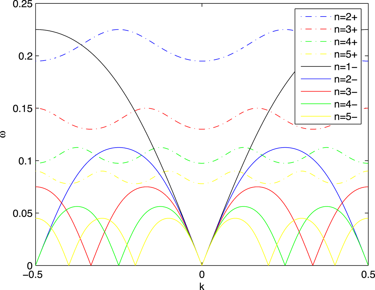
In this section we study the existence of nonresonant Lyapunov families of monochromatic wave trains in the MiM lattice. The range of $g_{\pm }(k,\,n)$ in (1.5) consists of two disjoint frequency bands. We distinguish between optical modes (corresponding to the dashed line in figure 1) and acoustic modes (corresponding to the solid line in figure 1). Assume that $k^*$
 and $\omega ^*$
 solve the equation $\omega ^*=g_{\pm }(k^*,\,n)$
 for exactly one pair $n=\pm n^*\in \mathbb {Z}_{\neq 0}$
 . Then both $\mathcal {K}$
 and $\mathcal {K}^*$
 are two-dimensional.
Theorem 3.1 Let $k^*\in [-1/2,\,1/2]$ and $\omega ^*>0$
 be such that $\omega ^*= g_{\pm }(k^*,\,n^*)$
 , but $\omega ^*\neq g_{\pm }(k^*,\,n)$
 for all $n\in \mathbb {Z}_{>0}\setminus \{n^*\}$
 . Then for every $\varepsilon \geq 0$
 close enough to 0 and every $\phi _0\in \mathbb {R}/2\pi \mathbb {Z}$
 there is a unique analytic function $\omega =\omega (\varepsilon )$
 such that $h_x(x_{n^*},\,x_{-n^*},\,\omega (\varepsilon ),\,k^*)=0$
 for every small $x_{n^*}=\frac {\varepsilon }{2}\mathrm {e}^{\mathrm {i}\phi _0}$
 and $\lim _{\varepsilon \rightarrow 0}\omega (\varepsilon )=\omega ^*$
 .
The dispersion curves $\omega =g_{\pm }(k,\,n)$ for $n=1,\,2,\,3,\,4,\,5$
 , where $\mu =0.5,\,\kappa =2$
 . $\omega =g_{-}(k,\,n)$
 (respectively, $\omega =g_+(k,\,n)$
 ) is shown in solid (respectively, dashed) curve.

Proof. It follows from the $\mathbb {S}^1\oplus \mathbb {Z}_2$ -invariant of $h$
 that it is a smooth function of $\omega,\,k$
 and the invariant $a=x_{n^*}x_{-n^*}$
 . Thus the reduced bifurcation equations $h_x(x_{n^*},\,x_{-n^*},\,\omega,\,k)=0$
 imply $x_{n^*}\frac {\partial h}{\partial a}=x_{-n^*}\frac {\partial h}{\partial a}=0$
 . So it is true that $\frac {\partial h}{\partial a}=0$
 except when $x_{n^*}=x_{-n^*}=0$
 .
In the following, we Taylor expand $h$ near $(x_{n^*},\,x_{-n^*},\,\omega ^*,\,k^*)=(0,\,0,\,\omega ^*,\,k^*)$
 . For this purpose, we shall for $u\in \mathscr {X}^l=\mathcal {K}\oplus \mathcal {M}^*$
 write

Note that the variables $x_{\pm n^*}$ are used to describe the elements of $\mathcal {K}$
 while the others describe the elements of $\mathcal {M}^*$
 . And $h$
 is obtained from $\tilde {H}$
 by viewing in $\tilde {H}$
 the dependent variables $x_n(n\neq \pm n^*)$
 and $y_{i,n}$
 as functions of the independent variables $x_{\pm n^*},\,\omega,\,k$
 for $\mathcal {K}\times \mathbb {R}^2$
 . These functions are defined by the equation $PF(u(x_{n^*},\,x_{-n^*},\,\omega,\,k),\,\omega,\,k)=0$
 . Differentiation of this equation gives that $x_n=\mathcal {O}(\|(x_{n^*},\,x_{-n^*},\,\omega -\omega ^*,\,k-k^*)\|^2)$
 for $n\neq \pm n^*$
 and $y_{i,n}=\mathcal {O}(\|(x_{n^*},\,x_{-n^*},\,\omega -\omega ^*,\,k-k^*)\|^2)$
 for all $n$
 . In terms of the variables $x_n,\,y_{i,n}(i=1,\,2,\,3),\,\omega$
 and $k$
 , the Hamiltonian function $\tilde {H}$
 reads

Then we have

Therefore, we see that $\frac {\partial ^2 h}{\partial \omega \partial a}\Big |_{a=0,\omega =\omega ^*}\neq 0$ . By means of the implicit function theorem, we can for every small positive value of $a=\frac {\varepsilon ^2}{4}$
 , find an $\omega =\omega (\varepsilon )$
 such that $h_x(\frac {\varepsilon }{2}\mathrm {e}^{\mathrm {i}\phi _0},\,\omega (\varepsilon ),\,k^*)=0$
 .
It follows from $u\in \mathcal {K}$ that

then the solutions are exactly of the form given in theorem 1.1. In summary, for every fixed $k^*$ there exists a one-parameter family of wave trains with amplitude $\varepsilon$
 .
4. Bichromatic wave trains
In figure 1, we can clearly see that several dispersion curves intersect transversally. For example, the curve $\omega =g_+(k,\,2)$ (the blue dashed line) and the curve $\omega =g_{-}(k,\,1)$
 (the black solid line) intersect at some point $(\omega ^{*},\,k^*)$
 and no other curves pass through this point. This is the 1:2 resonance. We can also find other resonant situations such as $1:3$
 , $2:3$
 and $2:5$
 resonances and so on.
Throughout this section, we always assume that
(H) There exist two distinct integers $p< q\in \mathbb {Z}_{>0}$
and parameters $\omega ^*>0$ and $k^*\in [-1/2,\,1/2]$ such that $\omega ^*= g_{\pm }(k^*,\,p)$ and $\omega ^*=g_{\pm }(k^*,\,q)$, but $\omega ^*\neq g_{\pm }(k^*,\,n)$ for all $n\in \mathbb {Z}_{>0}\setminus \{p,\,q\}$.


Under assumption (H), both $\mathcal {K}$ and $\mathcal {K}^*$
 are four-dimensional. Let $\mathrm {gcd}(p,\,q)$
 be the greatest common divisor of $p$
 and $q$
 , and define

The invariance of $h$ under the action of the time shift operator $R_{\alpha }$
 implies that $h$
 must be a smooth function of $\omega,\,k$
 and the invariants

Clearly, $a,\,b,\,c,\,d$ are all real when $x_{p}=\overline {x_{-p}}$
 and $x_{q}=\overline {x_{-q}}$
 , i.e. $(u_1,\,u_2,\,u_3,\,u_4)$
 is real-valued. In addition, the invariants have the following relation

and $\varrho$ acts on them as follows

In fact, $h$ is either a smooth function of $(a,\,b,\,c,\,\omega,\,k)$
 if $p+q$
 is odd, or a smooth function of $(a,\,b,\,d,\,\omega,\,k)$
 if $p+q$
 is even. Set

Then $h$ can be considered as a function of $(a,\,b,\,C,\,\omega,\,k)$
 . For convenience, we rewrite the potential function as

where $\gamma =\frac {{\rm d}^{\tilde {p}+\tilde {q}-1}V}{dz^{\tilde {p}+\tilde {q}-1}}(0)$ and $\delta =\frac {{\rm d}^{\tilde {p}+\tilde {q}}V}{{\rm d}z^{\tilde {p}+\tilde {q}}}(0)$
 . Let

for $\varsigma _1$ , $\varsigma _2$
 , $\varsigma _3$
 , $\varsigma _4\in \{a,\,b,\,\omega,\,k\}$
 .
Theorem 4.1 Under assumption (H), function $h$ has the following properties:
(i) The matrix
(4.2)\begin{equation} \mathcal{H}_{a,b,\omega,k}=\left[ \begin{array}{@{}cc@{}} \dfrac{\partial^2 h}{\partial a\partial\omega} & \dfrac{\partial^2 h}{\partial b\partial\omega}\\ \dfrac{\partial^2 h}{\partial a\partial k} & \dfrac{\partial^2 h}{\partial b\partial k}\\ \end{array} \right]_{(a,b,C,\omega,k) =(0,0,0,\omega^*,k^*)} \end{equation}is invertible if and only if the curves $\omega =g_{\pm }(k,\,p)$
and $\omega =g_{\pm }(k,\,q)$ intersect transversely at $(k^*,\,\omega ^*)$.(ii) if $\sin (p\pi k^*)\sin (q\pi k^*)\neq 0$
, then $\frac {\partial h}{\partial C}(0,\,0,\,0,\,\omega ^*,\,k^*)$ is a function of $(\gamma,\,\alpha,\,\beta,\,\cdots,\,\delta )$. In fact, this function is of the form $\frac {\partial h}{\partial C}(0,\,0,\,0,\,\omega ^*,\,k^*)=g(\gamma,\,\alpha,\,\beta,\,\cdots )+\varsigma \delta$, where $\varsigma$ is a nonzero constant and $g$ is some smooth function.


Proof. (i) Firstly, we expand $(u_1,\,u_2,\,u_3,\,u_4)\in \mathscr {X}^l =\mathcal {K}\oplus \mathcal {M}^*$ similarly to formula (3.1). Then the variables $\{z_{p},\,z_{-p},\,z_{q},\,z_{-q}\}$
 are used to describe the elements of $\mathcal {K}$
 while the others describe the elements of $\mathcal {M}^*$
 . Recall that $x_n\ (n\neq \pm p,\,\pm q)$
 and $y_{i,n}$
 can all be viewed as functions of the six independent coordinates $x_n\ (n=\pm p,\,\pm q),\,\omega,\,k$
 satisfying $x_n=\mathcal {O}(\|(x_{p},\,x_{-p},\,x_{q},\,x_{-q},\,\omega ^*-\omega,\,k^*-k)\|^2)$
 for $n\neq \pm p,\,\pm q$
 and $y_{i,n}=\mathcal {O}(\|(x_{p},\,x_{-p},\,x_{q},\,x_{-q},\,\omega ^*-\omega,\,k^*-k)\|^2)$
 for all $n$
 and $i\in \{1,\,2,\,3\}$
 . Then one obtains from (3.2) that

It follows that the determinant of matrix (4.2) is nonzero exactly when the derivatives of $k\mapsto g_{\pm }(k,\,p)$ and $k\mapsto g_{\pm }(k,\,q)$
 at $k^*$
 are different.
(ii) In this part, we set $\omega =\omega ^*$ and $k=k^*$
 and obtain the implicit equations for the dependent variables $x_n(n\neq \pm p,\,\pm q)$
 and $y_{i,n}$
 in terms of the independent variables $x_{\pm p},\,x_{\pm q}$
 . It suffices to prove the theorem under the assumption that $V(z)=\frac {1}{2}z^2+\frac {\delta }{(\tilde {p}+\tilde {q})!}z^{\tilde {p}+\tilde {q}}$
 . Equating all inner products of $F(U,\,\omega ^*,\,k^*)$
 with basis vectors for $\mathcal {M}$
 to zero yields that for $n\neq \pm p,\,\pm q$
 ,

and for $n=\pm p,\,\pm q$ ,

where

when $\tilde {p}+\tilde {q}$ is even, and

when $\tilde {p}+\tilde {q}$ is odd and $\overline {m}=(m_1,\,m_2,\,\cdots,\,m_{\tilde {p}+\tilde {q}-1})$
 . It follows from these equations that for all $n,\,m\in \mathbb {Z}$
 and $i\in \{1,\,2,\,3\}$
 ,

where $\delta _m^n$ is the Kronecker delta. Hence, $D_n=\mathcal {O}(\|(x_p,\,x_{-p},\,x_q,\,x_{-q})\|^{\tilde {p}+\tilde {q}-1})$
 . Then $x_n=\mathcal {O}(\|(x_p,\,x_{-p},\,x_q,\,x_{-q})\|^{\tilde {p}+\tilde {q}-1})$
 for $n\neq \{\pm p,\,\pm q\}$
 and $y_{i,n}=\mathcal {O}(\|(x_p,\,x_{-p},\,x_q, x_{-q})\|^{\tilde {p}+\tilde {q}-1})$
 for all $n$
 and $i\in \{1,\,2,\,3\}$
 . Now we again compute the reduced Hamiltonian function $h(\cdot,\,\omega ^*,\,k^*)$
 :

The function $g(a,\,b)$ appears only when $\tilde {p}+\tilde {q}$
 is even, and the plus or minus sign depends on the exact values of $\tilde {p}$
 and $\tilde {q}$
 . We have here used the fact that when $\sum _{j=1}^l m_j=0$
 , then

Note that $n$ satisfying

has the property $\Gamma _{\kappa,\mu }^{n,\omega ^*}\neq 0$ . Hence,

if $\sin (p\pi k^*)\sin (q\pi k^*)\neq 0$ . This completes the proof.
Note that $\tilde {p}\geq 1$ from figure 1. Then we distinguish two cases: $\tilde {p}>1$
 and $\tilde {p}=1$
 .
4.1. Case 1: $\tilde {p}>1$

In this case, we have the following result.
Theorem 4.2 Resonant wave trains
In addition to assumption (H) and $\tilde {p}>1$ . Assume that the curves $\omega ^*=g_{\pm }(k,\,p)$
 and $\omega ^*=g_{\pm }(k,\,q)$
 intersect transversely at $(k^*,\,\omega ^*)$
 and $\sin (p\pi k^*)\sin (q\pi k^*)\neq 0$
 . Then there are unique analytic functions $\omega _{\pm }=\omega _{\pm }(\varepsilon )$
 and $k_{\pm }=k_{\pm }(\varepsilon )$
 satisfying

such that the local solution set to the bifurcation equation $d_xh(x_p,\,x_{-p},\,x_q,\,x_{-q}, \omega,\,k)=0$ is given by

for $0<\varepsilon _1,\,\varepsilon _2<\varepsilon$ small enough, and $\phi _0\in \mathbb {R}/2\pi \mathbb {Z}$
 , $\eta _+=\frac {\pi }{2\tilde {p}},\, \eta _-=-\frac {\pi }{2\tilde {p}}$
 if $\tilde {p}+\tilde {q}$
 is odd, whereas $\eta _+=0,\,\eta _-=\frac {\pi }{\tilde {p}}$
 if $\tilde {p}+\tilde {q}$
 is even.
The proof is based on the implicit function theorem, which is similar to that theorem 7.2 in [Reference Guo, Lamb and Rink10], and hence is omitted.
4.2. Case 2: $\tilde {p}=1$

In the case where $\tilde {p}=1$ , we divide our analysis into three subcases: $\tilde {q}=2,\,\tilde {q}=3$
 and $\tilde {q}\geq 4$
 . Firstly, we shall treat the case that $\tilde {p}+\tilde {q}$
 is even. Note that $x_p=\overline {x_{-p}}$
 , $x_q=\overline {x_{-q}}$
 , then equations $d_xh(x_p,\,x_{-p},\,x_q,\,x_{-q},\,\omega,\,k)=0$
 read

By applying $\mathbb {S}^1$ -action, we assume that $x_p=x_1>0$
 , where $x_1\in \mathbb {R}$
 . Dividing by $x_1$
 the first equation of (4.5), shows that the remaining periodic solutions may be found by solving


Separating the real and imaginary parts of equation (4.6) gives $\frac {\partial h}{\partial d}\mathrm {Im}(x_q)=0$ . It follows from theorem 4.1 that $\frac {\partial h}{\partial d}(0,\,0,\,0,\,\omega ^*,\,k^*)\neq 0$
 , then we have $\mathrm {Im}(x_q)=0$
 . So $x_q$
 can be replaced by a real number $x_2$
 . Then (4.6) and (4.7) can be rewritten as

In the case where $\tilde {p}+\tilde {q}$ is odd, the analysis is completely similar, except that $\mathrm {Re}(x_q)=0$
 , and $x_q$
 can be replaced by $-\mathrm {i}x_2$
 . Then equation $d_xh(x_p,\,x_{-p},\,x_q,\,x_{-q},\,\omega,\,k)=0$
 can be rewritten as

In summary, equation $d_xh(x_p,\,x_{-p},\,x_q,\,x_{-q},\,\omega,\,k)=0$ can be reduced to


where $C=c$ if $\tilde {p}+\tilde {q}$
 is odd and $C=d$
 if $\tilde {p}+\tilde {q}$
 is even. Since $\frac {\partial ^2 h}{\partial a\partial \omega }(0,\,0,\,0,\,\omega ^*,\,k^*)\neq 0$
 , we can solve equation (4.8) for $\omega$
 based on the implicit function theorem, and then substitute this solution for $\omega$
 into (4.9). Thus finding the desired families of periodic solutions reduces to solving (4.9), where $h$
 is the function of $x_1^2,\,x_2^2,\,x_1^{\tilde {q}}x_2,\,\omega,\,k$
 , and $\omega =\omega (x_1^2,\,x_2^2,\,x_1^{\tilde {q}-2}x_2,\,k)$
 . Hence, (4.9) can be rewritten uniquely as

where $s(0,\,0,\,k)=0$ .
Next, we find solutions to (4.10) by using singularity theory to determine all small amplitude solutions. For this purpose, we consider the following Taylor expansions for $r$ and $s$
 at $(0,\,0,\,k^*)$
 :

where $u=x_1^2$ , $v=x_2^2$
 . The lowest coefficients of $r$
 and $s$
 with respect to $u$
 and $v$
 are given as follows:

The singularity theory has two main theorems that are used to determine the norm form of $W(x_1,\,x_2,\,k)$ . The following preliminaries can be found in Chapter 3 in [Reference Golubitsky and Schaeffer9]. Let $\mathcal {E}_{x,\lambda }$
 denote the space of all functions $g:\mathbb {R}^2\rightarrow \mathbb {R}$
 that are defined and $C^\infty$
 on some neighbourhood of the origin. We shall identify any two functions in $\mathcal {E}_{x,\lambda }$
 which are equal as germs. Let $T(g)$
 be the ‘tangent space’ of a germ $g$
 , which we defined formally as follows.
Definition 4.3 The tangent space to a germ $g$ in $\mathcal {E}_{x,\lambda }$
 consists of all germs of the form

where $a,\,b\in \mathcal {E}_{x,\lambda }$ and $c\in \mathcal {E}_\lambda$
 .
The tangent space constant theorem states that if $T(g+tp)=T(g)$ for all $t\in [0,\,1]$
 and $p\in \mathcal {E}_{x,\lambda }$
 , then $g+tp$
 is equivalent to $g$
 for all $t\in [0,\,1]$
 . The universal unfolding theorem states that if there exist $k$
 germs $p_1,\,\cdots,\,p_k\in \mathcal {E}_{x,\lambda }$
 such that

Then $G(x,\,\lambda,\,\alpha )=g+\sum _{j=1}^k\alpha _jp_j$ is a universal unfolding of $g$
 . First, we allow a more general system of coordinate changes:

where $X_2(0,\,0)\neq 0$ . This change of coordinates preserves the $x_2$
 axis. Meanwhile, when $\tilde {q}=2$
 , we require that $X_3(0,\,0)=0$
 , due to the fact that $s(0,\,0,\,0)=0$
 . It is not difficult to check that these transformations preserve the form of $W$
 and hence can be thought of as operations on the pair $(r(u,\,v),\,s(u,\,v))$
 . In the context of the theory developed in Golubitsky and Schaeffer [Reference Golubitsky and Schaeffer9], one finds that $T(W)$
 is a module of function pairs in $(\mathcal {E}_{u,v},\,\mathcal {M}_{u,v})$
 , where $\mathcal {E}_{u,v}$
 is the ring of germs of smooth, real-valued functions in the variables $u,\,v$
 and $\mathcal {M}_{u,v}\subset \mathcal {E}_{u,v}$
 is the maximal ideal generated by functions vanishing at the origin. Following the results in Theorems 18.1–18.3 in [Reference Golubitsky, Marsden, Stewart and Dellnitz8], this module has the following generators:
(i) when $\tilde {q}\geq 4$
, the generators are $(r,\,s),\,(u^{\tilde {q}-2}s,\,vr)$, $(2ur_u,\,2us_u+(\tilde {q}-2)s)$, $(2vr_v+r,\,2vs_v),\,(2u^{\tilde {q}-2}s_v,\,2vr_v+r)$.(ii) when $\tilde {q}=2$
, the generators are $(r,\,s)$, $(s,\,vr)$, $(2ur_u,\,2us_u)$, $(2vr_v+r,\,2vs_v)$, $(2uvs_v,\,2uv^2r_v+uvr)$.(iii) when $\tilde {q}=3$
, the generators are $(r,\,s)$, $(us,\,vr)$, $(2ur_u,\,2us_u+s)$, $(2vr_v+r,\,2vs_v)$, $(2us_v,\,2vr_v+r)$, $(2u^2s_u+us,\,2uvr_u)$.


Based on the tangent space constant theorem and the universal unfolding theorem, we have
Lemma 4.4
(i) Assume that $\tilde {q}\geq 4$
. If $a_1,\, b_1,\, a_2,\, b_2$ and $a_1b_2-3b_1a_2$ are nonzero. Then the bifurcation equation $W=0$ is equivalent to the normal form
(4.11)\begin{equation} x_1^2x_2+\varepsilon x_2^3+k x_2+x_1^{\tilde{q}}=0, \end{equation}where $\varepsilon =\pm 1$
.(ii) Assume that $\tilde {q}=3$
. If $b_1$ and $\chi \triangleq (2b_2^3-9a_1b_1b_2+27b_1^2a_2)$ are nonzero, then $W=0$ is equivalent to the normal form
(4.12)\begin{equation} x_1^3+mx_1^2x_2+x_2^3+k x_2=0, \end{equation}where
\[ m=3\mathrm{sgn}(\chi)\frac{3a_1b_1-b_2^2}{\chi^{2/3}} \]is a modal parameter.
(iii) Assume that $\tilde {q}=2$
. If $a_2,\,b_2$ are nonzero, then $W=0$ is equivalent to the normal form
(4.13)\begin{equation} \varepsilon x_1^2+x_2^2+k x_2=0, \end{equation}where $\varepsilon =\pm 1$
.


Remark 4.5 Note that when $\tilde {q}=2$ and $\tilde {q}\geq 4$
 , the codimension of $T(W)$
 is one, and the unfolding parameter is $k$
 ; when $\tilde {q}=3$
 , the codimension of $T(W)$
 is two, one is the modal parameter $m$
 and the other is $k$
 . The detailed proof of lemma 4.4 is given in § 18 in [Reference Golubitsky, Marsden, Stewart and Dellnitz8] and hence omitted here.
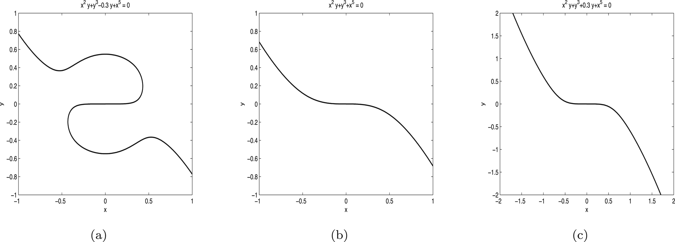
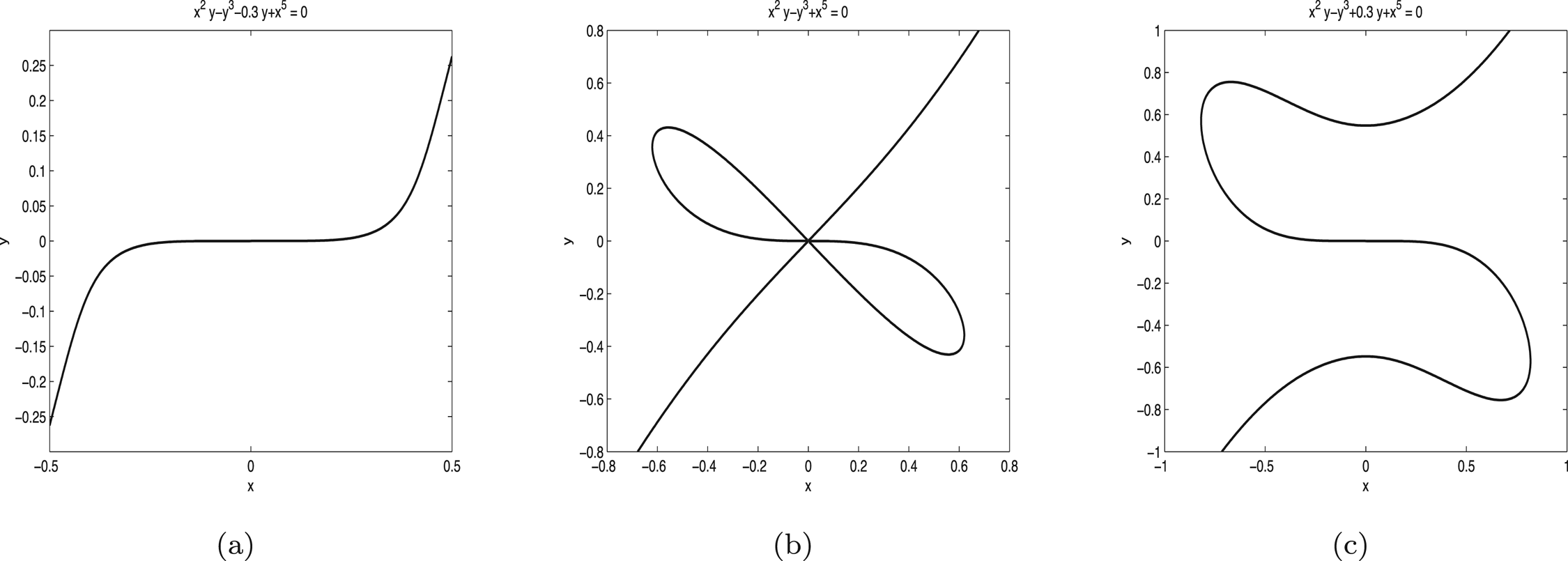
Now we consider the solutions that may be derived from the normal forms in the previous lemma. For the case $\tilde {q}\geq 4$ , equation (4.11) yields the pictures in figures 2 and 3. In the case where $\tilde {q}=3$
 , the pictures of equation (4.12) are similar to figure 2 for all $m\in \mathbb {R}$
 . In the case where $\tilde {q}=2$
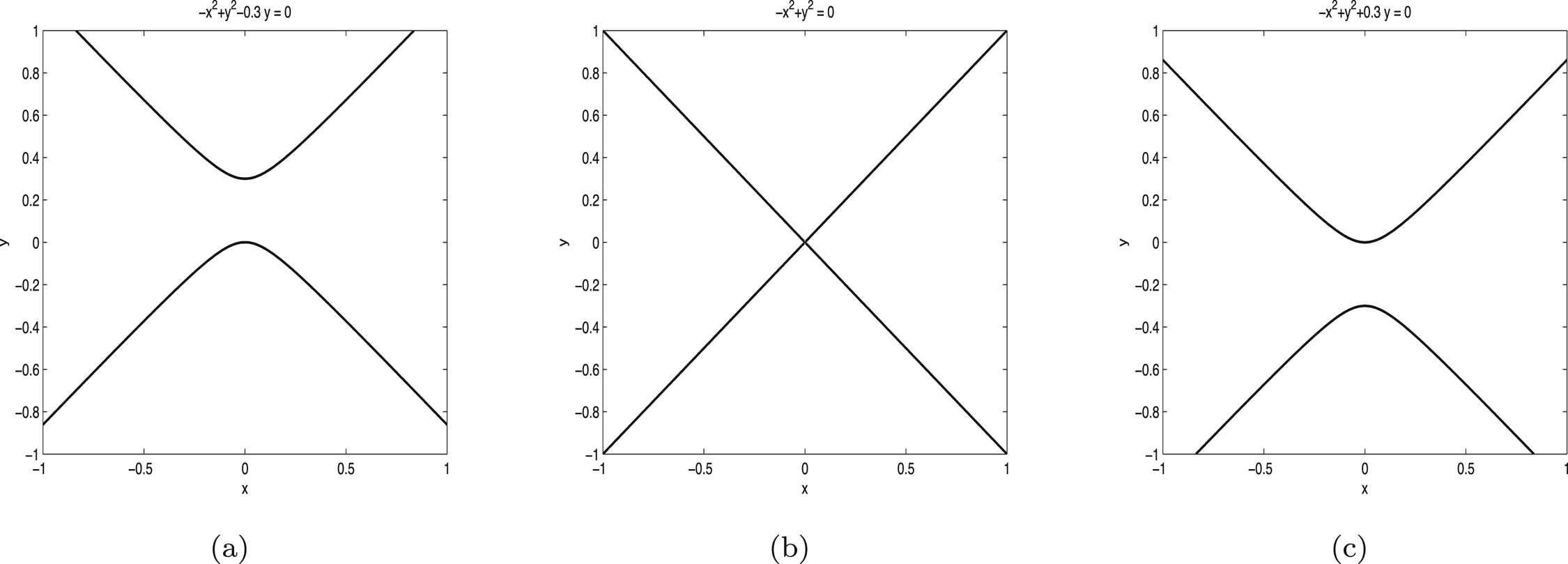
 , equation (4.13) is graphed in figures 4 and 5.
Theorem 4.6 In addition to conditions (H), assume that $\tilde {q}\geq 4$ and $a_1,\, b_1,\, a_2,\, b_2$
 and $a_1b_2-3b_1a_2$
 are nonzero.
(i) Equation (4.11) with $\varepsilon =1$
and $k<0$ has three distinct zeros when $x_1$ varies in some sufficiently small right neighbourhood of 0. Thus, system (1.1) may have three distinct branches of periodic solutions of form (1.7) as $(\omega,\,k)$ varies in some sufficiently small neighbourhood of $(\omega ^*,\,k^*)$.(ii) Equation (4.11) with $\varepsilon =1$
and $k\geq 0$ has only one zero. Thus, system (1.1) may have only one branch of periodic solution of form (1.7) as $(\omega,\,k)$ varies in some sufficiently small neighbourhood of $(\omega ^*,\,k^*)$.(iii) Equation (4.11) with $\varepsilon =-1$
and $k<0$ has only one zero when $x_1$ varies in some sufficiently small right neighbourhood of 0. Thus, system (1.1) may have one branch of periodic solutions of form (1.7) as $(\omega,\,k)$ varies in some sufficiently small neighbourhood of $(\omega ^*,\,k^*)$.(iv) Equation (4.11) with $\varepsilon =-1$
and $k\geq 0$ has three distinct zeros. Thus, system (1.1) may have three distinct branches of periodic solutions of form (1.7) as $(\omega,\,k)$ varies in some sufficiently small neighbourhood of $(\omega ^*,\,k^*)$.


Equation $x^2y+\varepsilon y^3+ky+x^{\tilde {q}}=0$ with $\varepsilon =1$
 and $\tilde {q}=5$
 .

Equation $x^2y+\varepsilon y^3+ky+x^{\tilde {q}}=0$ with $\varepsilon =-1$
 and $\tilde {q}=5$
 .

Equation $\varepsilon x^2+y^2+ky=0$ with $\varepsilon =-1$
 .

Equation $\varepsilon x^2+y^2+ky=0$ with $\varepsilon =1$
 .

In the case where $\tilde {q}=3$ , the bifurcation pictures are essentially the same to those in the case where $\tilde {q}\geq 4$
 and $\varepsilon =1$
 . Thus, the results are similar and hence is omitted.
Theorem 4.7 Under assumptions (H), assume that $\tilde {q}=2$ and $a_2,\,b_2$
 are nonzero.
(i) Equation (4.13) with $\varepsilon =1$
and $k\neq 0$ has two zeros when $x_1$ varies in some sufficiently small right neighbourhood of 0. This means that system (1.1) may have two branches of periodic solutions of form (1.7) as $(\omega,\,k)$ varies in some sufficiently small neighbourhood of $(\omega ^*,\,k^*)$.(ii) Equation (4.13) with $\varepsilon =-1$
has two distinct zeros when $x_1$ varies in a sufficiently small right neighbourhood of 0. Thus, system (1.1) may have two distinct branches of periodic solutions of form (1.7) as $(\omega,\,k)$ varies in some sufficiently small neighbourhood of $(\omega ^*,\,k^*)$.


We remark that the change of the sign of $k$ may affect the number of branches of solutions for the norm forms in the case where $\tilde {q}\geq 4$
 . This means that the number of branches of bichromatic wave trains may change as $k$
 goes across $k^*$
 for system (1.1) under the assumptions of theorem 4.6. However, the bichromatic wave trains in theorem 1.2 are always unique up to a phase shift as $k$
 goes across $k^*$
 .
5. Discussion
By means of Lyapunov–Schmidt reduction and singularity theory, we obtain the small-amplitude solutions near equilibria in nonresonance and $p:q$ resonance, respectively. In particular, the monochromatic and bichromatic wave trains persist near $\mu =0$
 in the nonresonance case and the resonance case $p:q$
 where $q$
 is not an integer multiple of $p$
 . Namely, the wave trains of the MiM lattice shadows that of the corresponding monatomic FPU lattice under the nondegeneracy conditions. In addition, we show the multiplicity of bichromatic wave trains in the resonance case $p:q$
 , where $q$
 is an integer multiple of $p$
 .
Notice that $k$ must be nonzero in the resonance case. In other words, when $k^*=0$
 and $\omega ^*>0$
 , system (1.1) only admits the monochromatic wave trains of form (1.6). Moreover, system (1.1) also has the following solution:

where $y(t)$ is a periodic function and $\nu \in \mathbb {R}$
 . Substituting of (5.1) into (1.1), we obtain the following equation for $y(t)$
 :

Notice that the parameter $\nu$ do not enter in (5.2) because (1.1) is invariant under the transformation

Since $\kappa >0,\,\mu >0$ , equation (5.2) has the general solutions:

for any $c_1,\,c_2\in \mathbb {R}$ . It is easy to see that solution (5.1) belongs to solutions (1.4) with $k=0$
 . Therefore, the nonlinear MiM lattice (1.1) sustains binary oscillations of arbitrarily large amplitudes.
Now, we conclude this paper with some remarks. Note that the discussions in the resonance case $p:q$ where $q$
 is not an integer multiple of $p$
 in § 4 need the nondegeneracy condition (i) in theorem 4.1. If the nondegeneracy condition (i) does not hold, that is, the curves $\omega =g_{\pm }(k,\,p)$
 and $\omega =g_{\pm }(k,\,q)$
 are tangent to each other at the point $(k^*,\,\omega ^*)$
 , then it becomes more complicated and challenging to study the existence and multiplicity of bichromatic wave trains. Furthermore, there may be three distinct integers $p< q< r$
 and $\omega ^*>0$
 and $k^*\in (0,\,1/2]$
 such that $\omega ^*=g_{\pm }(k^*,\,p),\,\omega ^*=g_{\pm }(k^*,\,q),\,\omega ^*=g_{\pm }(k^*,\,r)$
 and $\omega ^*\neq g_{\pm }(k^*,\,n)$
 for all $n\in \mathbb {Z}_{>0}\setminus \{p,\,q,\,r\}$
 . Then the kernel $\mathcal {K}$
 becomes six-dimensional. It would be more interesting to investigate the existence and multiplicity of trichomatic wave trains.
For diatomic chains and MiM lattice, generic solitary waves are expected to be nonlocal, and the existence of such solutions has been proved only for certain asymptotic limits, summarized in [Reference Vainchtein24]. However, numerical and asymptotic results suggest that for a countable collection of antiresonance values of the system’s parameter, there are genuine solitary waves. There are a lot of research on wave trains and solitary waves of monatomic FPU chains ([Reference Filip and Venakides6, Reference Friesecke and Wattis7, Reference Herrmann12, Reference Pankov18, Reference Pankov and Rothos19, Reference Smets and Willem23]) and diatomic chains ([Reference Qin21, Reference Qin22]) with variational approaches. We expect that the variational approaches can also be extended to deal with the MiM lattice.
Acknowledgements
Research supported by the National Natural Science Foundation of P.R. China (grant Nos. 12371195 and 12071446) and the Fundamental Research Funds for the Central Universities, China University of Geosciences (Wuhan) (grant No. CUGST2)