



1 Introduction
Deep learning (Krizhevsky, Sutskever & Hinton Reference Krizhevsky, Sutskever and Hinton2012), reinforcement learning (Mnih et al. Reference Mnih, Kavukcuoglu, Silver, Rusu, Veness, Bellemare, Graves, Riedmiller, Fidjeland and Ostrovski2015) and their performance beyond human capabilities (He et al. Reference He, Zhang, Ren and Sun2015; Silver et al. Reference Silver, Huang, Maddison, Guez, Sifre, van den Driessche, Schrittwieser, Antonoglou, Panneershelvam and Lanctot2016, Reference Silver, Schrittwieser, Simonyan, Antonoglou, Huang, Guez, Hubert, Baker, Lai and Bolton2017) have been recently recognized. In particular, deep learning has shown amazing performance and evolved rapidly day by day, and has been widely applied in many areas as noted by LeCun, Bengio & Hinton (Reference LeCun, Bengio and Hinton2015). Inspired by this advancement, naturally arising questions in turbulence research would include ‘Can deep learning learn turbulence, which is infamously known to be a chaotic and strongly nonlinear phenomenon?’ and ‘If turbulence is learnable, what element of turbulence makes learning possible?’ In order to pursue answers to these questions, we applied deep learning to the prediction of turbulent heat transfer based only on wall-shear and pressure information in channel flow. We investigated whether deep learning can help us to quantify and physically understand the nonlinear relationship underlying turbulence data, which is not easily identified by conventional statistical methods.
Although the application of machine learning to fluid dynamics has become very active recently, the first attempt dates back to Lee et al. (Reference Lee, Kim, Babcock and Goodman1997), who applied an artificial neural network (ANN) to turbulence control for drag reduction. In their study, shallow learning was successfully applied to the prediction of the near-wall wall-normal velocity based on the wall-shear stresses or pressure. Since then, machine learning in various forms has been applied to diverse areas of fluid mechanics, such as flow reconstruction, unsteady flow prediction, flow control, finding solutions to nonlinear partial differential equations (PDEs) and turbulence modelling. For example, flow reconstruction from experimental data using ANNs based on radial basis functions (Pruvost, Legrand & Legentilhomme Reference Pruvost, Legrand and Legentilhomme2001; Hočevar, Širok & Grabec Reference Hočevar, Širok and Grabec2005), turbulence reconstruction from noise-added isotropic and stratified turbulence using an ANN (Maulik & San Reference Maulik and San2017) and flow prediction around a bluff body using the dimension reduction machine learning method (Bright, Lin & Kutz Reference Bright, Lin and Kutz2013) and convolutional neural networks (CNNs) (Miyanawala & Jaiman Reference Miyanawala and Jaiman2017; Jin et al. Reference Jin, Cheng, Chen and Li2018; Lee & You Reference Lee and You2018) were carried out. In order to predict flow information recursively, Hennigh (Reference Hennigh2017) and Mohan & Gaitonde (Reference Mohan and Gaitonde2018) used autoencoder (AE) architectures composed of convolution layers, and Mohan & Gaitonde (Reference Mohan and Gaitonde2018) and Wang et al. (Reference Wang, Xiao, Fang, Govindan, Pain and Guo2018) used long short-term memory (LSTM), too. Similarly, Lusch, Kutz & Brunton (Reference Lusch, Kutz and Brunton2018) applied the AE for the prediction of relatively simple nonlinear dynamics, finding out that the dynamics can be globally linear on the low dimension. Flow control has been one of the active areas and has seen various applications of machine learning (Milano & Koumoutsakos Reference Milano and Koumoutsakos2002; Lorang, Podvin & Quéré Reference Lorang, Podvin and Quéré2008; Duriez et al. Reference Duriez, Parezanovic, Laurentie, Fourment, Delville, Bonnet, Cordier, Noack, Segond and Abel2014; Gautier et al. Reference Gautier, Aider, Duriez, Noack, Segond and Abel2015; Rabault et al. Reference Rabault, Kuchta, Jensen, Réglade and Cerardi2019). A bold approach to solving nonlinear PDEs was made by Raissi, Yazdani & Karniadakis (Reference Raissi, Yazdani and Karniadakis2018) and Raissi et al. (Reference Raissi, Wang, Triantafyllou and Karniadakis2019), who applied deep neural networks to express the solutions of the Navier–Stokes equations in terms of spatial positions and time, and Bar-Sinai et al. (Reference Bar-Sinai, Hoyer, Hickey and Brenner2018), who used CNNs for an accurate discretization of spatial derivatives. In addition, ANNs are nowadays used as a part of the experimental workflows, especially in particle image velocimetry (Lee, Yang & Yin Reference Lee, Yang and Yin2017; Rabault, Kolaas & Jensen Reference Rabault, Kolaas and Jensen2017; Cai et al. Reference Cai, Zhou, Xu and Gao2019)
Another active area of the application of machine learning to fluid mechanics is turbulence modelling, such as large-eddy simulation (LES) (Sarghini, Felice & Santini Reference Sarghini, Felice and Santini2003; Gamahara & Hattori Reference Gamahara and Hattori2017; Vollant, Balara & Corre Reference Vollant, Balara and Corre2017; Beck, Flad & Munz Reference Beck, Flad and Munz2018; Maulik et al. Reference Maulik, San, Rasheed and Vedula2018, Reference Maulik, San, Rasheed and Vedula2019) and Reynolds-averaged Navier–Stokes (RANS) modelling (Tracey, Duraisamy & Alonso Reference Tracey, Duraisamy and Alonso2013, Reference Tracey, Duraisamy and Alonso2015; Duraisamy, Zhang & Singh Reference Duraisamy, Zhang and Singh2015; Ling & Templeton Reference Ling and Templeton2015; Zhang & Duraisamy Reference Zhang and Duraisamy2015; Ling, Jones & Templeton Reference Ling, Jones and Templeton2016a ; Ling, Kurzawski & Templeton Reference Ling, Kurzawski and Templeton2016b ; Parish & Duraisamy Reference Parish and Duraisamy2016; Kutz Reference Kutz2017; Ling et al. Reference Ling, Ruiz, Lacaze and Oefelein2017; Singh, Duraisamy & Zhang Reference Singh, Duraisamy and Zhang2017a ; Singh, Medida & Duraisamy Reference Singh, Medida and Duraisamy2017b ; Wang et al. Reference Wang, Wu, Ling, Iaccarino and Xiao2017a ; Wang, Wu & Xiao Reference Wang, Wu and Xiao2017b ; Wu et al. Reference Wu, Sun, Laizet and Xiao2017; Milani et al. Reference Milani, Ling, Saez-Mischlich, Bodart and Eaton2018; Sotgiu, Weigand & Semmler Reference Sotgiu, Weigand and Semmler2018; Wu, Xiao & Paterson Reference Wu, Xiao and Paterson2018; Duraisamy, Iaccarino & Xiao Reference Duraisamy, Iaccarino and Xiao2019), in which various attempts to improve the subgrid-scale model or the Reynolds stress models have been made. In addition to the above examples, physical interpretation of nonlinear turbulence using neural networks (Ferre-Gine et al. Reference Ferre-Gine, Rallo, Arenas and Giralt1996; Giralt et al. Reference Giralt, Arenas, Ferre-Gine, Rallo and Kopp2000) was carried out. Although practical applications of machine learning are indeed necessary, applications of machine learning for a more fundamental study of turbulence are equally useful, but quite rare.
In the present work, we used deep learning to predict the turbulent heat transfer (the wall-normal heat flux) on the basis of other wall information obtained by DNS of channel flow and also attempted to analyse the physics of the heat transfer through it. In channel flow, Antonia, Krishnamoorthy & Fulachier (Reference Antonia, Krishnamoorthy and Fulachier1988) and Kim & Moin (Reference Kim and Moin1989) found that temperature fluctuations are highly correlated with streamwise velocity fluctuations. Similarly, Abe, Kawamura & Matsuo (Reference Abe, Kawamura and Matsuo2004) reported that wall-normal heat flux fluctuations are mostly similar to streamwise wall-shear stress fluctuations regardless of the Reynolds number, but dissimilarity between them occurs in some regions, in which there are large wall pressure fluctuations. It is well known that the presence and behaviour of vortices near the wall are significant in near-wall transport. High streamwise wall-shear stress on the wall interacts with (is both affected by and affects) the streamwise vortices, and the correlation between them becomes maximum at the side downstream from the shear stress position (Kravchenko, Choi & Moin Reference Kravchenko, Choi and Moin1993). According to Abe & Antonia (Reference Abe and Antonia2009), when these vortices exist, large fluctuating streamwise and spanwise pressure gradients occur, and streamwise gradients intensify or weaken momentum streaks, unlike thermal streaks. From these observations, we hypothesized that the wall-normal heat flux can be explicitly expressed as nonlinear combinations of nearby streamwise wall-shear stress, spanwise wall-shear stress and pressure fluctuations, which can be captured by deep learning. If this hypothesis is true, turbulent heat transfer could be obtained from just the wall information. Then, the trained network might contain information on the physical correlation of the heat transfer; therefore, an analysis of the network may help us to figure out the physical characteristics.
Explicit correlation between the heat transfer and wall information, such as shear stresses or pressure, would be beneficial for practical applications. It is well known that the prediction of turbulent heat transfer in RANS/LES simulations, which are frequently adopted in many industrial applications, is much less accurate than the prediction of skin friction. The construction of a successful machine learning network to accurately predict heat transfer on the basis of wall information would greatly enhance the usefulness of RANS/LES. For example, accurate wall-normal heat flux might be predicted from the wall-shear stresses and pressure obtained by RANS on coarse grids through training the network with RANS and DNS datasets. Such a possibility is discussed in this paper. Furthermore, correct identification of the role of vortices in the heat transfer mechanism would help in the design of artificially generated vortices for heat transfer augmentation (Fiebig Reference Fiebig1995; Jacobi & Shah Reference Jacobi and Shah1995). To date, various types of vortex generators (Torii, Kwak & Nishino Reference Torii, Kwak and Nishino2002; Ahmed, Mohammed & Yusoff Reference Ahmed, Mohammed and Yusoff2012; Liu & Sakr Reference Liu and Sakr2013; Gallegos & Sharma Reference Gallegos and Sharma2017; Alam & Kim Reference Alam and Kim2018) have been studied numerically and experimentally to develop the heat exchangers used in various fields. Therefore, identifying the relationship between the vortex and heat transfer is crucial not only for a fundamental understanding of turbulent physics but also for many practical applications.
This article presents deep learning procedures in § 2, results and discussion in § 3 and conclusions in § 4. In § 2.1, turbulent channel flow simulations based on a spectral method for collecting the data used for deep learning are introduced. In § 2.2, our CNN architecture and network optimization process are described. The resulting prediction accuracy for several Reynolds numbers is presented in § 3.1. In §§ 3.2 and 3.3, observations of inaccurately predicted cases and gradient maps of the trained network are provided. Finally, the possibility that our CNN could be utilized as a turbulence model is discussed in § 3.4.
2 Deep learning procedures
2.1 Data collection by DNS
In order to collect deep learning datasets, DNS of fully developed turbulent channel flow with a passive temperature field were carried out. Mean flow in the
 $x$
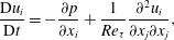
-direction is driven by the mean pressure gradient, and the temperature distribution is developed by the temperature difference between the top and bottom walls. The governing equations are the continuity equation, the incompressible Navier–Stokes equations and the energy equation:
 $$\begin{eqnarray}\displaystyle & \displaystyle \frac{\unicode[STIX]{x2202}u_{i}}{\unicode[STIX]{x2202}x_{i}}=0, & \displaystyle\end{eqnarray}$$
 $$\begin{eqnarray}\displaystyle & \displaystyle \frac{\text{D}u_{i}}{\text{D}t}=-\frac{\unicode[STIX]{x2202}p}{\unicode[STIX]{x2202}x_{i}}+\frac{1}{Re_{\unicode[STIX]{x1D70F}}}\frac{\unicode[STIX]{x2202}^{2}u_{i}}{\unicode[STIX]{x2202}x_{j}\unicode[STIX]{x2202}x_{j}}, & \displaystyle\end{eqnarray}$$
 $$\begin{eqnarray}\displaystyle & \displaystyle \frac{\text{D}T}{\text{D}t}=\frac{1}{PrRe_{\unicode[STIX]{x1D70F}}}\frac{\unicode[STIX]{x2202}^{2}T}{\unicode[STIX]{x2202}x_{j}\unicode[STIX]{x2202}x_{j}}. & \displaystyle\end{eqnarray}$$
Here
 $x_{i}$
,
 $u_{i}$
and
 $T$
are the coordinates, velocity and temperature variables normalized by the channel half-width (
 $\unicode[STIX]{x1D6FF}$
), the friction velocity (
 $u_{\unicode[STIX]{x1D70F}}$
) and half the temperature difference (
 $\unicode[STIX]{x0394}T$
) between the top and bottom walls, respectively;
 $x_{1}$
(
 $x$
),
 $x_{2}$
(
 $y$
) and
 $x_{3}$
(
 $z$
) denote the streamwise, wall-normal and spanwise directions; and the corresponding velocity components are
 $u_{1}$
(
 $u$
),
 $u_{2}$
(
 $v$
) and
 $u_{3}$
(
 $w$
), respectively. The dimensionless parameters are the frictional Reynolds number (
 $Re_{\unicode[STIX]{x1D70F}}$
), which is defined by
 $u_{\unicode[STIX]{x1D70F}}$
,
 $\unicode[STIX]{x1D6FF}$
and the kinetic viscosity
 $\unicode[STIX]{x1D708}$
, and the Prandtl number (
 $Pr=\unicode[STIX]{x1D708}/\unicode[STIX]{x1D6FC}$
), which is fixed as
 $0.71$
, with
 $\unicode[STIX]{x1D6FC}$
denoting the thermal diffusivity.
Simulation parameters for DNS.

Periodic boundary conditions are imposed in the horizontal directions, and the no-slip and constant-temperature conditions are applied at the wall. To numerically solve the governing equations, a pseudo-spectral method with the Fourier expansion for the horizontal directions and the Chebyshev-tau method for the wall-normal direction is used. For time advancement, the third-order Runge–Kutta scheme and the Crank–Nicolson scheme are employed for the nonlinear terms and the viscous terms, respectively. The domain size and the number of grid points for each Reynolds number are listed in table 1, which are greater than or equal to those of Moser, Kim & Mansour (Reference Moser, Kim and Mansour1999). The code has been validated by application to various problems (Yeo, Kim & Lee Reference Yeo, Kim and Lee2009, Reference Yeo, Kim and Lee2010; Lee & Lee Reference Lee and Lee2015; Park & Lee Reference Park and Lee2015; Jang & Lee Reference Jang and Lee2018).
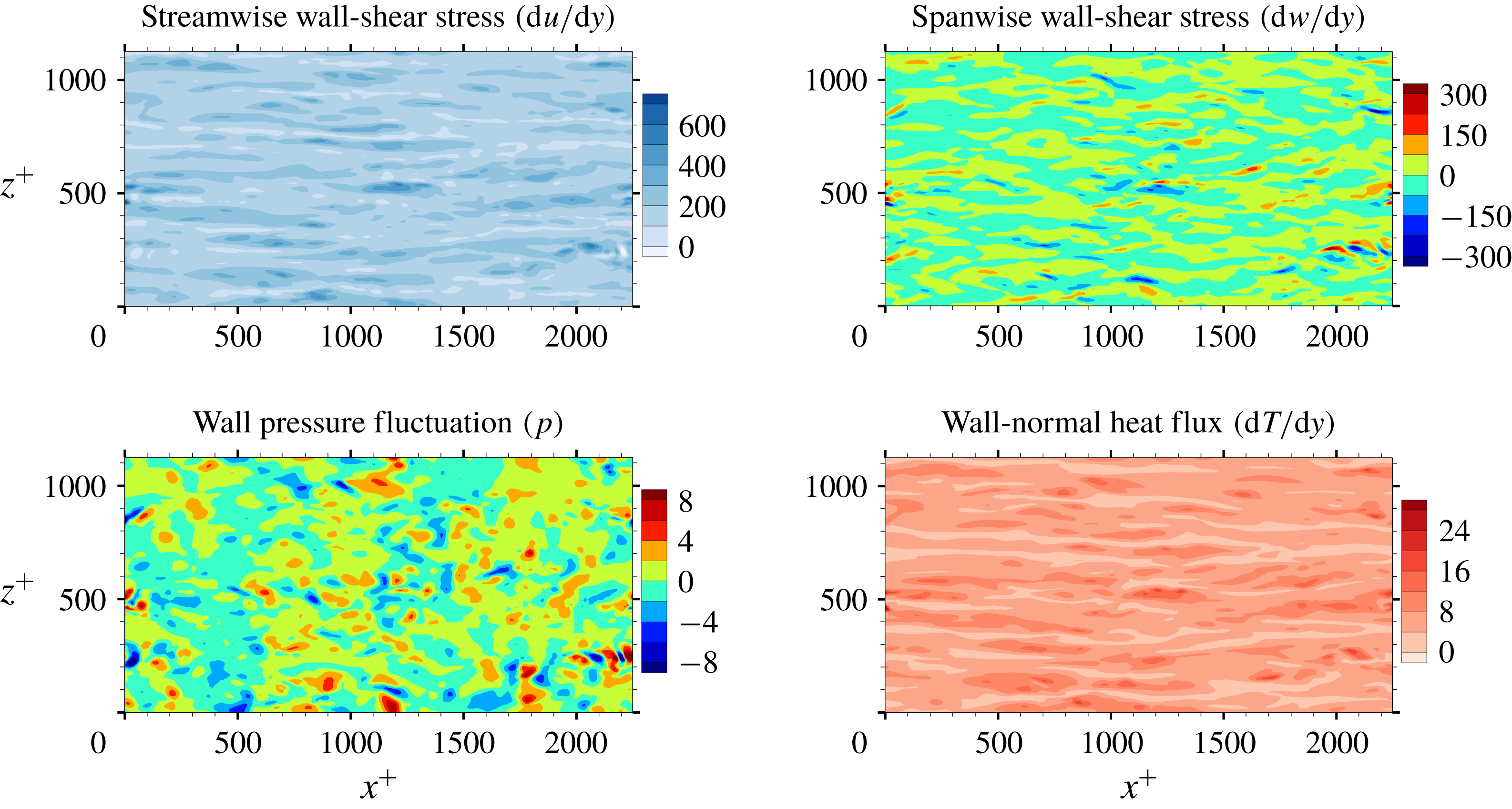
Wall information extracted from DNS that is used for the input and output of a deep learning network. The streamwise wall-shear stress, spanwise wall-shear stress and wall pressure fluctuation are the inputs, and the wall-normal heat flux is the target of deep learning. Here, the spanwise wall-shear stress is referred to as the streamwise wall vorticity.
The data at
 $Re_{\unicode[STIX]{x1D70F}}=180$
are used for training, validation and testing, and the data at the other
 $Re_{\unicode[STIX]{x1D70F}}$
are used for testing only. In table 1,
 $Nu$
denotes the Nusselt number, which is the normalized average heat transfer in the wall-normal direction. As proposed by Kasagi, Tomita & Kuroda (Reference Kasagi, Tomita and Kuroda1992), in the channel flow simulation, the Nusselt number can be well fitted by a linear function of the Reynolds number:
 $$\begin{eqnarray}Nu\approx 0.0284Re_{\unicode[STIX]{x1D70F}}+1.\end{eqnarray}$$
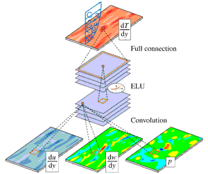
As shown in figure 1, we collected four types of wall information, including the streamwise wall-shear stress (interchangeably called the shear stress)
 $\text{d}u/\text{d}y$
, the spanwise wall-shear stress (or vorticity)
 $\text{d}w/\text{d}y$
and the wall pressure fluctuations
 $p$
as inputs, and the wall-normal heat flux
 $\text{d}T/\text{d}y$
as the prediction target. In order to train the deep learning network with statistically independent data, fields were collected per
 $\unicode[STIX]{x0394}t^{+}=36$
, which is longer than the integral lifetime scale of the spanwise wall-shear and pressure (Quadrio & Luchini Reference Quadrio and Luchini2003). A total of 6400 training fields were accumulated. The size of the training data in the single precision is approximately 3.7 GB. Further, in channel flow, the mirror image of the collected data can be used as the training data by taking advantage of the statistical symmetry between
 $(x,y,z)$
and
 $(x,y,-z)$
. This data augmentation method is expected to help prevent overfitting in addition to imposing symmetry on the deep learning network, and can be critical for a situation where the amount of collected data is insufficient. Although not used in this study, spectral shifting can also be used for data augmentation in the present problem. As a preprocess, the inputs of training data are normalized to have
 $\text{mean}=0$
and
 $\text{standard deviation}=1$
:
 $$\begin{eqnarray}x_{train}^{\prime }=\frac{x_{train}-\unicode[STIX]{x1D707}(x_{train})}{\unicode[STIX]{x1D70E}(x_{train})},\end{eqnarray}$$
where
 $x_{train}$
,
 $x_{train}^{\prime }$
,
 $\unicode[STIX]{x1D707}$
and
 $\unicode[STIX]{x1D70E}$
are the original training data, preprocessed training data, mean and standard deviation of the original training data, respectively.
2.2 Deep learning model: CNN
Among the many types of deep learning algorithm, the CNN proposed by LeCun (Reference LeCun1989) has recently shown remarkable performance, particularly in image classification such as AlexNet (Krizhevsky et al. Reference Krizhevsky, Sutskever and Hinton2012), ZFNet (Zeiler & Fergus Reference Zeiler and Fergus2014), VGGNet (Simonyan & Zisserman Reference Simonyan and Zisserman2014), GoogLeNet (Szegedy et al. Reference Szegedy, Liu, Jia, Sermanet, Reed, Anguelov, Erhan, Vanhoucke and Rabinovichw2015) and ResNet (He et al. Reference He, Zhang, Ren and Sun2015). In the present research, the wall-shear information can be regarded as two-dimensional images, similar to the RGB (red, green, blue) images of the classification problem. CNN is known to efficiently handle the spatial information in the input images to approximate the required output through highly nonlinear mapping. Therefore, we expected that CNN would be a proper model to predict the local value of the heat transfer based on the spatial features in the wall-shear stresses and pressure.
A typical CNN architecture consists of convolution layers, pooling layers and fully connected layers. The core layer is the convolution layer, in which the output calculated from the input images (maps) is maintained in the form of a two-dimensional image so that spatial information can be efficiently extracted. Kernels in the form of
 $3\times 3$
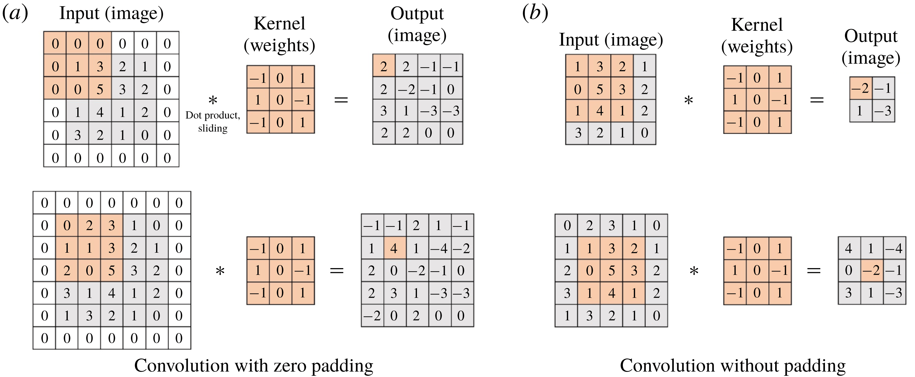
weights are convolved with the input fields, producing feature maps on the hidden layer. Here, zero padding is usually employed to maintain the same output size as the input size, but we did not use such a discontinuous application to break the smoothness of flow data. One characteristic of this discrete convolution operation without padding is that the input and output sizes can be varied, and the output from the small-size input can be a part of the output from the large-size input. For example, the convolution with zero padding can cause different parts of the output to be present at the same spatial location when the inputs have different sizes, as illustrated in figure 2(a). However, the convolution without padding results in the same output at the same location regardless of the input size. In other words, the small-size output is a part of the large-size output (figure 2
b). This property is useful for our problem, and the details are discussed later.
Padding effect of discrete convolution.
There is a problem called the internal covariate shift in which during training the input distribution in each layer can change, as the parameters in the previous layers change (Ioffe & Szegedy Reference Ioffe and Szegedy2015). To suppress this phenomenon, a batch normalization (Ioffe & Szegedy Reference Ioffe and Szegedy2015) that normalizes the input layer using the mean and variance, which are moving-averaged by batch datasets for training steps, is applied after each convolution. Next, a nonlinear function is used to impose nonlinearity in the network. The equations of this layer can be expressed as
 $$\begin{eqnarray}y_{conv}=\unicode[STIX]{x1D70E}(BN(w_{conv}\ast x_{conv})),\end{eqnarray}$$
where
 $x_{conv}$
,
 $w_{conv}$
,
 $BN$
,
 $\unicode[STIX]{x1D70E}$
and
 $y_{conv}$
are the input maps, kernels, batch normalization, nonlinear function and output feature maps, respectively. As the nonlinear function, an exponential linear unit (ELU) function (Clevert, Unterthiner & Hochreiter Reference Clevert, Unterthiner and Hochreiter2015) is used:
 $$\begin{eqnarray}\unicode[STIX]{x1D70E}(x)=\left\{\begin{array}{@{}ll@{}}x, & x\geqslant 0,\\ \text{e}^{x}-1, & x<0.\end{array}\right.\end{eqnarray}$$
This nonlinear function is smooth and expected to be effective in separating turbulent structures of the input such as low- and high-speed streaks, and positive and negative parts of pressure and vorticity. Although a rectified linear unit (ReLU) function is commonly used in image classification, it can eliminate a large amount of information from the input. Therefore, we used the smooth ELU function, which is expected to work a little better for the flow data. In fact, we tried both and found that the ELU function performs slightly better than the ReLU function.
The pooling layer usually extracts only important information so that the size of the input maps is reduced. However, because too much information in the maps can be lost, we do not use this layer. Finally, the fully connected layer connects all components of the feature maps generated through several convolution layers with the output:
 $$\begin{eqnarray}y_{fc}=\sum w_{fc}\,x_{fc}+b_{fc},\end{eqnarray}$$
where
 $x_{fc}$
,
 $w_{fc}$
,
 $b_{fc}$
and
 $y_{fc}$
are the input maps, weights, biases and output of the fully connected layer, respectively. Through the last fully connected layer, a single value of the wall-normal heat flux is predicted.
Before training the constructed network, we first define the loss function, which is defined by the sum of the data loss (
 $L_{i}$
) and the regularization loss (
 $R(w)$
) to prevent overfitting:
 $$\begin{eqnarray}L_{total}=\frac{1}{N}\mathop{\sum }_{i=1}^{N}L_{i}+\unicode[STIX]{x1D706}R(w),\end{eqnarray}$$
where
 $$\begin{eqnarray}\displaystyle & \displaystyle L_{i}=(y_{i}^{DNS}-y_{i}^{CNN})^{2}, & \displaystyle\end{eqnarray}$$
 $$\begin{eqnarray}\displaystyle & \displaystyle R(w)=\frac{1}{2}\mathop{\sum }_{k}w_{k}^{2}. & \displaystyle\end{eqnarray}$$
Here
 $y_{i}^{DNS}$
is the wall-normal heat flux from DNS;
 $y_{i}^{CNN}$
is the predicted value from the CNN;
 $k$
denotes the index of the weights in the network;
 $N$
is the batch size, which denotes the number of datasets used in a training step; and
 $\unicode[STIX]{x1D706}$
is the weight decay parameter, which is fixed as 0.0001. Minimizing this loss function is expected to enable the network to produce good predictions for testing. A commonly used method to minimize the loss is the gradient descent method, which iteratively updates the parameters in the network in the negative direction of the total loss gradient. The gradient can be obtained by the chain rule, whose details are demonstrated well by LeCun et al. (Reference LeCun, Bengio and Hinton2015), and the parameters are updated by the product of the gradient and the learning rate. The larger the learning rate set, the larger the resulting parameter change. The initial learning rate is set to
 $0.0005$
, and we reduce the learning rate by
 $1/5$
per
 $400$
epochs, and the total number of epochs is 2000. Here, one epoch means the period for which the given training datasets are used all at once for training. One of the gradient descent methods, adaptive moment estimation (ADAM) (Kingma & Ba Reference Kingma and Ba2014), which is known to show good convergence and requires little hyperparameter tuning, is used. The open-source library TensorFlow (Abadi et al.
Reference Abadi, Agarwal, Barham, Brevdo, Chen, Citro, Corrado, Davis, Dean and Devin2015) is used to train the CNN.
Modified CNN architecture composed of only convolution layers without zero padding, which is more cost-efficient than the classical architecture shown above because there is no redundant application of the convolution layers. In the modified architecture, the output size is variable with a choice of the input size.

The architecture of the network employing the CNN needs to be briefly discussed. We wanted to construct a network to predict the heat flux at a single position on the basis of the shear stresses and pressure distribution in a nearby rectangular region with size
 $N_{x}\times N_{z}$
. Here,
 $N_{x}$
and
 $N_{z}$
are the number of grid points in the streamwise and spanwise directions, respectively. In this study, the input kernel size
 $N_{x}\times N_{z}$
is mostly fixed to
 $33\times 33$
. Then, in order to predict a heat flux field on a grid of size
 $192\times 192$
, one has to provide an
 $N_{x}\times N_{z}$
size input
 $192\times 192$
times, which is greatly inefficient. However, it can be noticed that predicting the heat flux at the adjacent points requires the input data, whose share of data is large. An example is illustrated in the classical architecture of figure 3, where two input images having the same partial information pass through convolution layers without zero padding, and then identical parts (the black dashed line) in the output feature maps are produced. We can reduce the cost by calculating these overlapped parts only once. To achieve this, we removed the fully connected layer of the classical CNN architecture and added the convolution layer operated by the same number of weights as the fully connected layer. Therefore, the modified CNN performs an identical operation as that of the classical CNN on the input kernel of
 $N_{x}\times N_{z}$
size. However, there is a big difference that the input kernel size can be varied from
 $N_{x}\times N_{z}$
to a maximum of
 $(N_{x}+191)\times (N_{z}+191)$
, and the corresponding output size is varied from
 $1$
to
 $192\times 192$
. For example, by providing an
 $N_{x}\times (N_{z}+1)$
size input to the CNN instead of providing an
 $N_{x}\times N_{z}$
size input twice, the heat flux at the two spanwise-adjacent points can be obtained without any redundant calculation. This modified CNN can quickly predict a heat flux field by using an
 $(N_{x}+191)\times (N_{z}+191)$
input only once.
A total of 12 800 fields – including the collected data and the reflected data using the mirror image, which contains
 $12\,800\times 192\times 192~(=471\,859\,200)$
datasets – were used for training. During the training, we set the size of the input images to
 $(N_{x}+191)\times (N_{z}+191)$
instead of
 $N_{x}\times N_{z}$
as discussed above. This can yield a similar effect to setting a large batch size and thus help quick learning in the constructed network. Keskar et al. (Reference Keskar, Mudigere, Nocedal, Smelyanskiy and Tang2016) reported a problem that the test accuracy of the network trained with a large batch size is worse than that for the one with a small batch size, but this problem did not occur in the present study. The test accuracy of our approach is good, and this method is critically fast for cases that require training of a large amount of data or cases in which the input kernel size (
 $N_{x}\times N_{z}$
) is large. For training of our networks, the batch size is fixed as four fields (
 $=4\times 192\times 192$
); i.e. the networks are trained using four fields per iteration.
In the network that we are constructing, a number of important hyperparameters need to be determined before training, such as the input kernel size (
 $N_{x}\times N_{z}$
), the number of convolution layers, the number of maps in each convolution layer and the convolution kernel size. We first set the input kernel size as
 $33\times 33$
, i.e. approximately
 $389\times 194$
in wall units, from the observation that a streak of the wall heat flux is fully captured in that size. The kernel size in a convolution operation is fixed as
 $3\times 3$
, the size used in VGGNet (Simonyan & Zisserman Reference Simonyan and Zisserman2014). In order to find appropriate values of the other hyperparameters, a grid searching method is used. As the number of convolution layers is varied among three, six and nine, we changed the number of feature maps in the convolution layers from four to 32. Then, we observed training and validation errors calculated using
 $20$
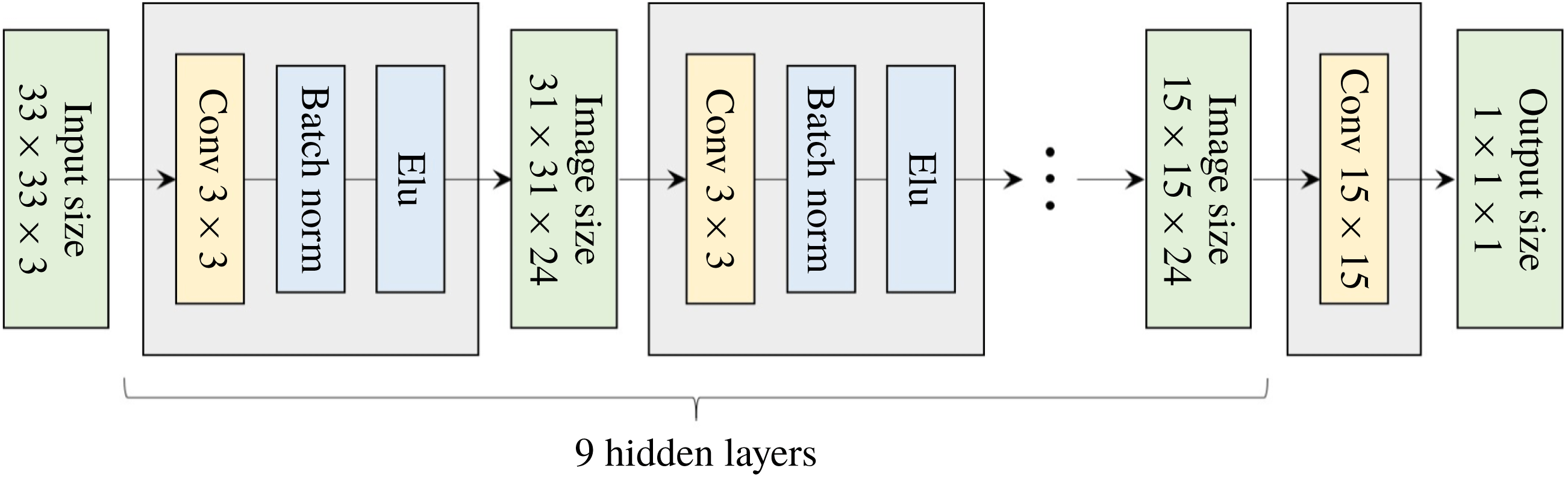
fields that are not among the trained data fields and are sufficiently far away from the training fields. When overfitting, which makes the validation error much larger than the training error, seemed to occur, we increased the number of training datasets and checked the errors again. The results are given in figure 4, and validation errors are sometimes smaller than the corresponding training errors because validation data are randomly selected turbulence data. As the number of feature maps increases, the validation errors decrease and converge to a specific value. When the number of maps is the same, the validation errors with six convolution layers are rather smaller than the errors with three convolution layers (not shown here), but the errors with six and nine convolution layers are almost the same. The results indicate that the depth and width of the network are large enough for the prediction of the local heat flux based on the given inputs. This also means that the heat flux sometimes cannot be expressed by a unique function in terms of the inputs because considerable errors remain. From the above process, an optimal structure of the network among the trained networks is determined, and consists of nine
 $3\times 3$
convolution layers, 24 feature maps in each convolution layer and one final
 $15\times 15$
convolution layer, as shown in figure 5. The total number of weights in the optimal network is approximately 48 000, which is not an extremely large number. Our optimal network was trained for 103 h on a single GPU server (NVIDIA Titan Xp) to obtain the best results. However, while performing a quick training in practical applications, 5 h are enough to guarantee good prediction accuracy close to that of the optimized one.
Mean square error (MSE) of the networks composed of (a) six convolution layers and (b) nine convolution layers with the number of feature maps changed in each convolution layer. For cases where overfitting occurred, we increased the number of original training fields from
 $3200$
to
 $6400$
. The validation errors of a simple linear regression using a single point of shear stress as input and a multiple linear regression using a stencil of shear stresses and pressure are approximately
 $1.05$
and
 $0.38$
, respectively.

Architecture of the optimized network. Here
 $33\times 33~(=N_{x}\times N_{z})$
is the input kernel size needed to predict a single point of output. According to the increase in the input size, the image size in the hidden layer and output size can increase.
3 Results and discussion
3.1 Test of the constructed network
First, the accuracy of the prediction by the trained network was validated against the DNS data at
 $Re_{\unicode[STIX]{x1D70F}}=180$
. The test data are apart from the training data more than 10 000 in wall time units. Fifty test fields were used, and the time interval between them is
 $90$
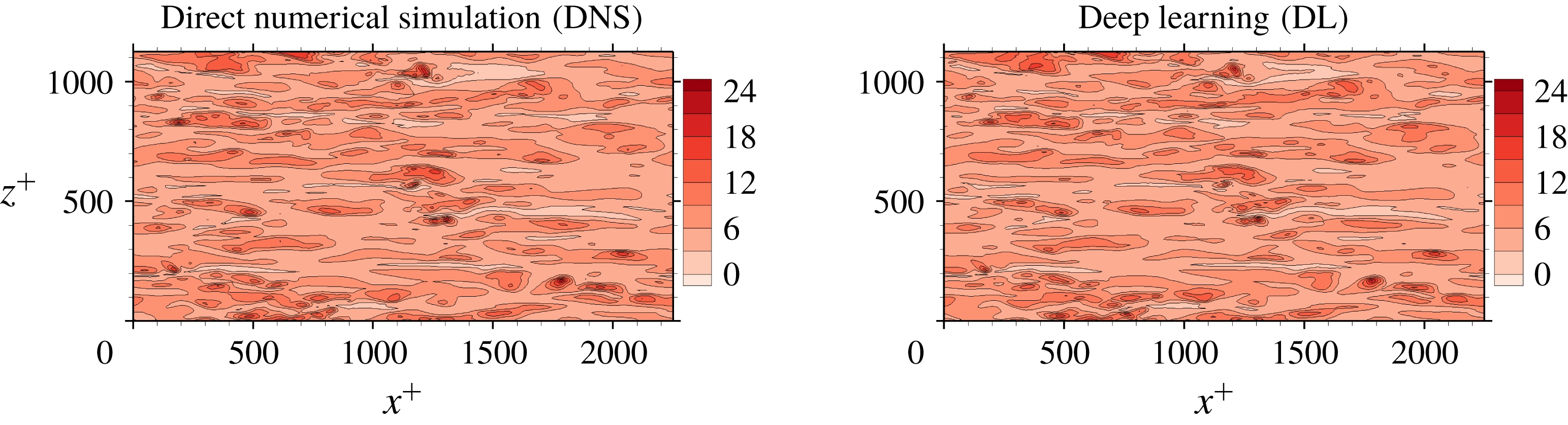
in wall time units, which guarantees that the data are almost uncorrelated with each other. An example comparison between the DNS result of the heat flux and the prediction through deep learning for a test field is presented in figure 6. It indicates that the shape of the structures and the local maximum locations of the prediction agree fairly well with those of the DNS. In order to quantify the prediction accuracy, we used a correlation coefficient (
 $R$
) between the DNS and the prediction values,
 $$\begin{eqnarray}R=\frac{\langle q_{w}^{DNS}q_{w}^{DL}\rangle }{q_{w,rms}^{DNS}q_{w,rms}^{DL}},\end{eqnarray}$$
Comparison of an instantaneous heat flux field between the DNS and the prediction by the trained deep learning network at the Reynolds number
 $Re_{\unicode[STIX]{x1D70F}}=180$
.
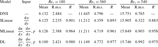
Test results of simple linear regression (SLinear), multiple linear regression (MLinear) and deep learning (DL) at three Reynolds numbers. The network was trained at
 $Re_{\unicode[STIX]{x1D70F}}=180$
, but tested at
 $Re_{\unicode[STIX]{x1D70F}}=180,~360$
and
 $540$
. For Reynolds numbers
 $Re_{\unicode[STIX]{x1D70F}}=360$
and
 $540$
, the same number of input kernel grid points (
 $N_{x}\times N_{z}=33\times 33$
) and the same grid size
 $((\unicode[STIX]{x0394}x^{+},\unicode[STIX]{x0394}z^{+})=(11.781,5.890))$
as those of the trained one (
 $Re_{\unicode[STIX]{x1D70F}}=180$
) were used.
where
 $q_{w}$
is the wall-normal heat flux fluctuations, defined as
 $q_{w}=(\text{d}T/\text{d}y)-\langle \text{d}T/\text{d}y\rangle$
, and
 $q_{w,rms}$
is the root-mean-square (r.m.s.) of
 $q_{w}$
. The angle bracket denotes the average over all test points. For the purpose of comparison, two kinds of linear regression models were considered. One is a simple linear regression (SLinear) using a single point data of the streamwise wall-shear stress as input; and the other is a multiple linear regression (MLinear) using the same inputs as the deep learning (DL). The validation errors of SLinear, MLinear and optimal DL are 1.05, 0.38 and 0.21, respectively (figure 4). Therefore, the test accuracy of DL was expected to be superior to those of the two linear models, especially for high heat flux regions. Quantified test results of the performances, including the mean, r.m.s. and
 $R$
, are shown in table 2. At the tested Reynolds number of 180, the mean values of the prediction by SLinear, MLinear and optimized DL are in very good agreement with those of the DNS. However, the r.m.s. values predicted by DL and MLinear are much closer to the value of the DNS than that of SLinear. The
 $R$
of
 $0.901$
between the DNS and the prediction by the SLinear was obtained at the Reynolds number of 180, indicating that there exists a pointwise correlation between the shear stress and the heat flux. However, it is not good enough for accurate prediction of the heat flux, because a deviation from the pointwise correlation is usually observed in the high-flux regions. On the other hand, from the optimized deep learning model, we obtained an
 $R$
of
 $0.980$
, finding that the deviation from the perfect correlation,
 $1-R$
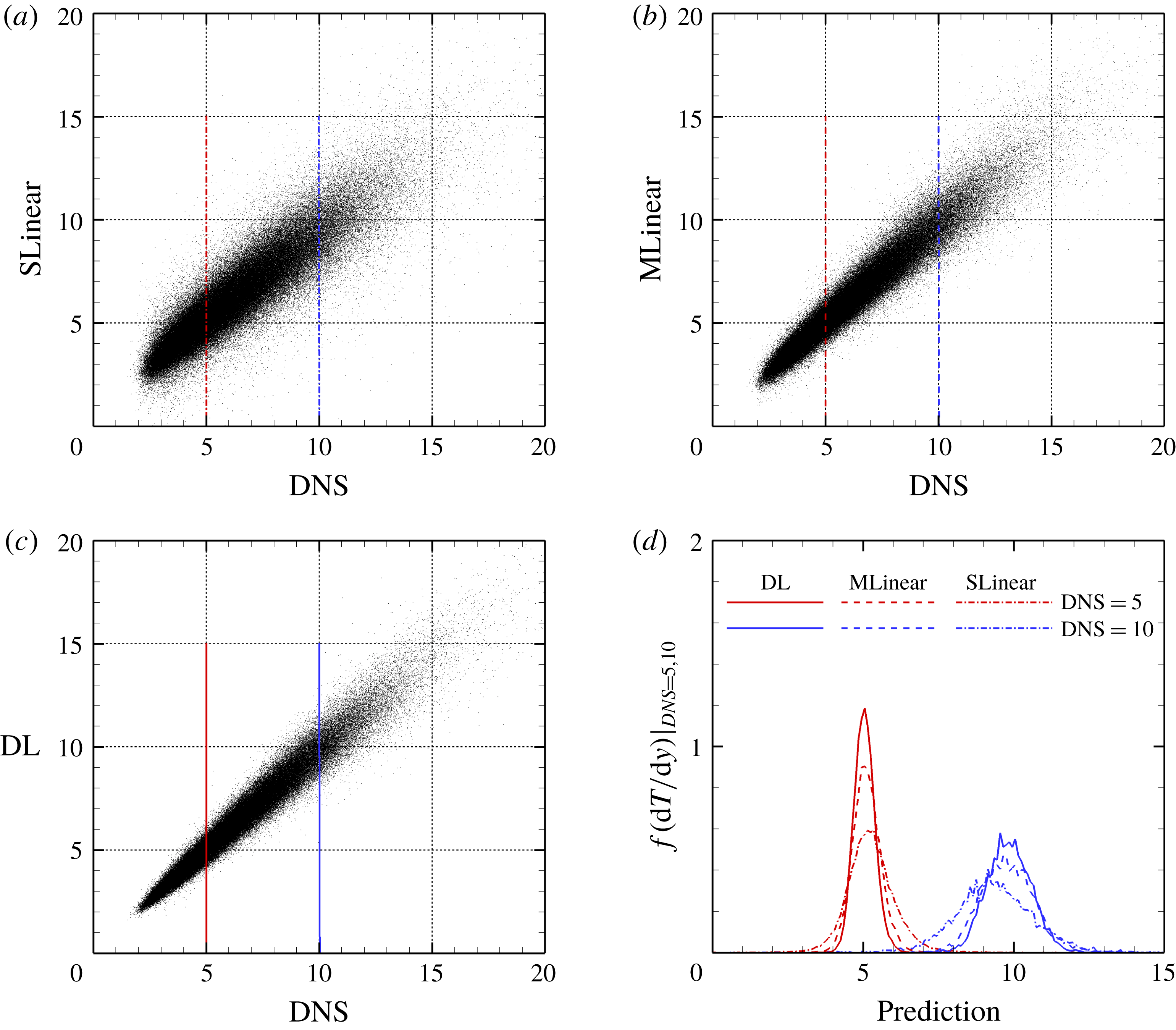
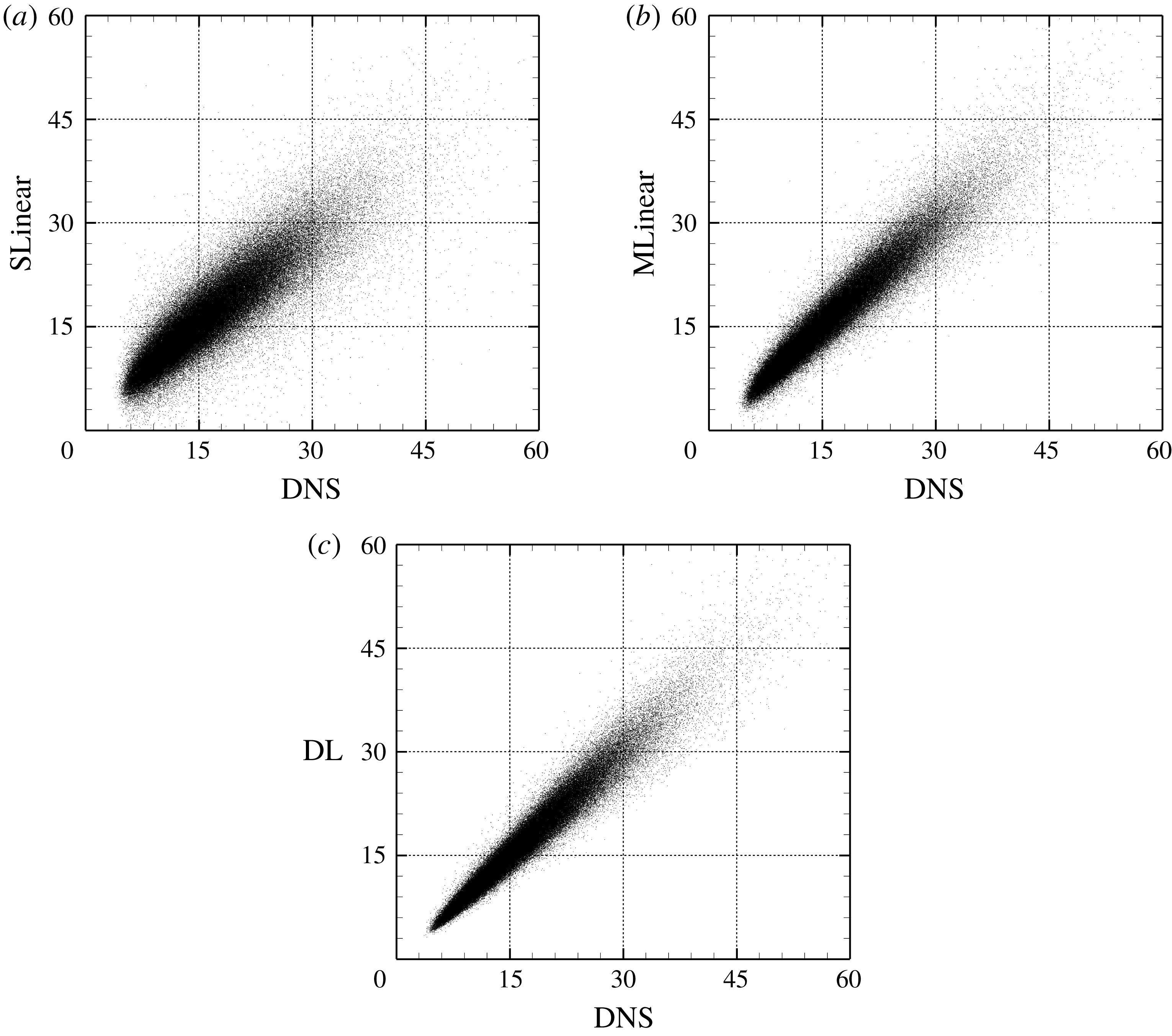
, is one-fifth of that from SLinear and approximately half of that from MLinear, clearly indicating that the nonlinear DL captures the correlation much better than both linear networks. Further, the scatterplots between the DNS and the predictions are given in figure 7, confirming that the prediction by DL is superior to that by both linear models. The cross-sectional distribution of the probability density functions (p.d.f.s) along the red (DNS value = 5) and blue (DNS value = 10) lines in figure 7(a–c) is also presented in figure 7(d), indicating that the peak values obtained by the DL are much higher than those obtained by both linear models. However, a trend is observed for the prediction of a large value: the performance deteriorates for all models.
Comparison of heat flux scatterplot between the DNS and prediction values for the trained Reynolds number using (a) SLinear, (b) MLinear and (c) DL. Only one-tenth of all test data are plotted. (d) The p.d.f.s of prediction data under the condition that the DNS value = 5 and 10. Here, conditioning was achieved by collecting data in the range
 $(5-0.1,5+0.1)$
and
 $(10-0.1,10+0.1)$
among all test data used for calculating the p.d.f.s.
(a) P.d.f.s and (b) high-order moments of the DNS and prediction for the trained Reynolds number.
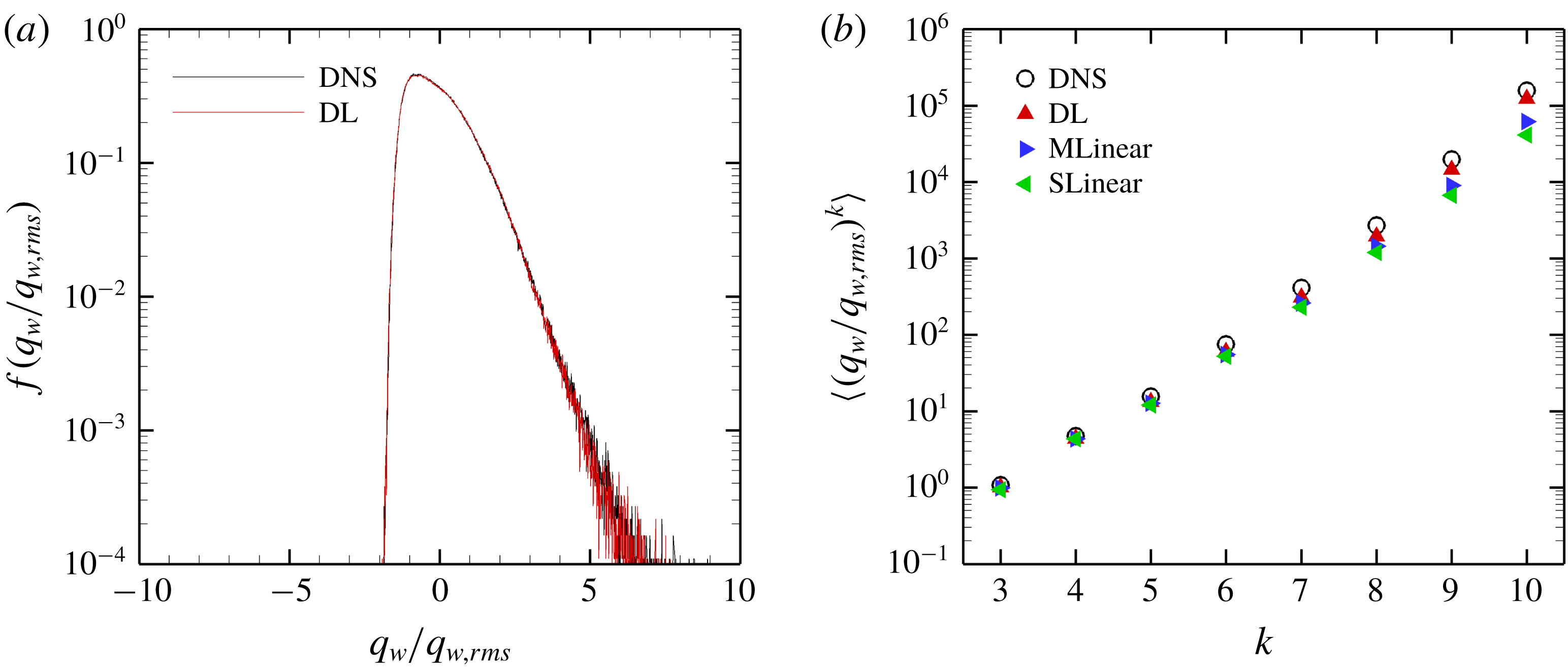
The total p.d.f.s and high-order moments of the heat flux data of the DNS and prediction by the models are compared in figure 8. The prediction of the p.d.f. by DL agrees well with the DNS results except for the very high heat flux parts. The moments predicted by DL are much closer to those of the DNS than those of the linear models even for a very high order. Although MLinear shows relatively higher prediction accuracy than SLinear, DL goes beyond it, especially for high heat flux. These results indicate that deep learning indeed captures well the nonlinear relation between the local heat flux and the spatial information of the shear stresses and pressure at the trained Reynolds number.
Comparison of heat flux scatterplot between the DNS and prediction values for the Reynolds number three times higher than the trained one using (a) SLinear, (b) MLinear and (c) DL.
(a) P.d.f.s of heat flux and (b) high-order moments of the DNS and prediction for the Reynolds number three times higher than the trained number.
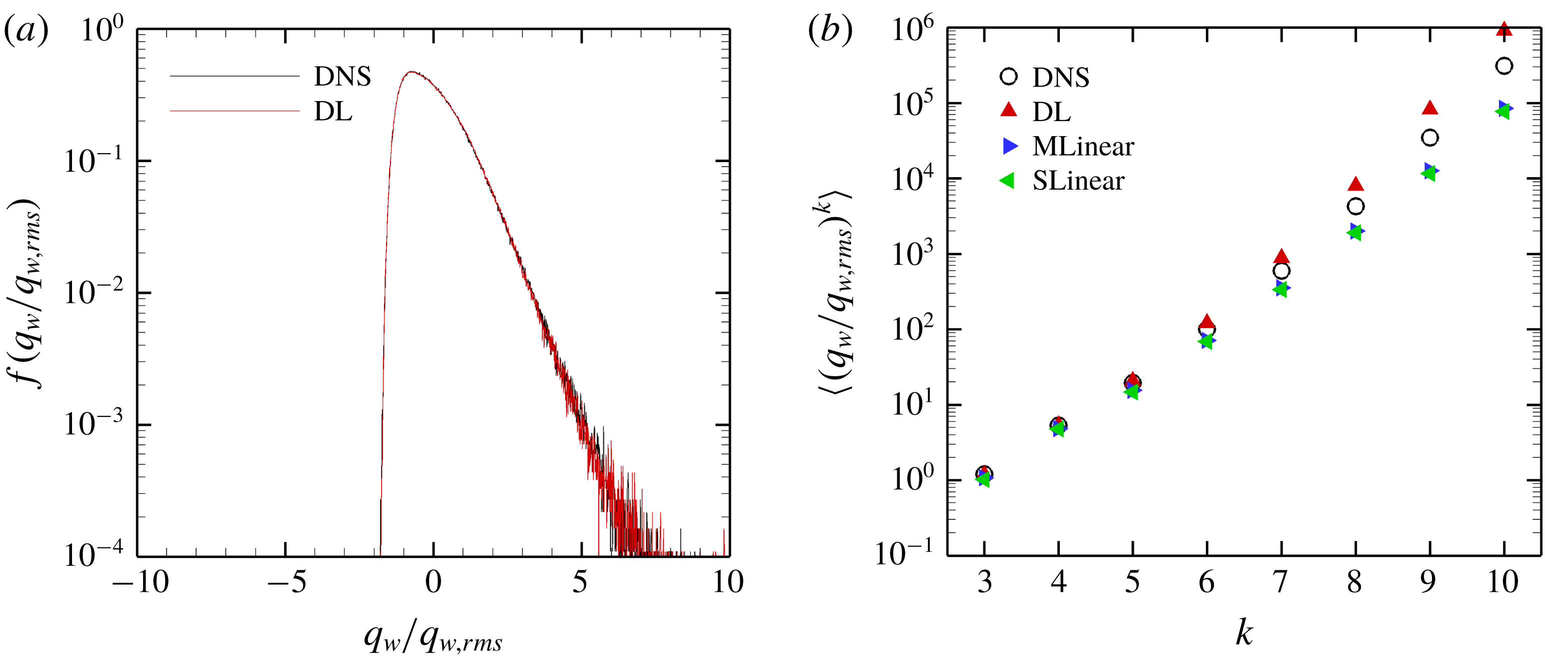
Next, we investigated whether the trained network can predict the turbulent heat transfer at other Reynolds numbers higher than the trained number. The data at other Reynolds numbers, however, have different scales from the trained number. The scales of the wall-shear stresses except pressure increase with the Reynolds number. Therefore, in order to match the input scales to the trained Reynolds number, the test input information except pressure is additionally rescaled by the ratio
 $Re_{\unicode[STIX]{x1D70F}}~(=Re_{\unicode[STIX]{x1D70F},test}/Re_{\unicode[STIX]{x1D70F},train})$
:
 $$\begin{eqnarray}x_{test}^{\prime }=\frac{x_{test}\displaystyle \frac{Re_{\unicode[STIX]{x1D70F},train}}{Re_{\unicode[STIX]{x1D70F},test}}-\unicode[STIX]{x1D707}(x_{train})}{\unicode[STIX]{x1D70E}(x_{train})}.\end{eqnarray}$$
Here
 $x_{test}$
and
 $x_{test}^{\prime }$
are the original input data and preprocessed input data at the tested Reynolds number, respectively; and
 $\unicode[STIX]{x1D707}(x_{train})$
and
 $\unicode[STIX]{x1D70E}(x_{train})$
are the mean and standard deviation of the training data, which were used in (2.5). Further, the target wall-normal heat flux at each
 $Re_{\unicode[STIX]{x1D70F}}$
has different scales. However, if the normalized input maps are used on the trained network, the output in the range of scales at the trained Reynolds number will be produced. To adjust the scales to the heat flux scales at other Reynolds numbers, the predicted outputs are normalized by the inverse ratio of the Nusselt number,
 $$\begin{eqnarray}y_{test}=y_{test}^{\prime }\frac{Nu_{test}}{Nu_{train}},\end{eqnarray}$$
where
 $y_{test}^{\prime }$
is the output of the network and
 $y_{test}$
is the scaled output, which has the scales at the tested Reynolds number. Because the Nusselt number can be well approximated by a simple function of the Reynolds number (2.4) within our simulated Reynolds-number range, it is reasonable to assume that we already know the Nusselt number at the other Reynolds numbers. In short, this simple scaling process is identical to using
 $(1/Re_{\unicode[STIX]{x1D70F}})\,\text{d}u/\text{d}y$
,
 $(1/Re_{\unicode[STIX]{x1D70F}})\,\text{d}w/\text{d}y$
and
 $(1/Nu)\,\text{d}T/\text{d}y$
instead of
 $\text{d}u/\text{d}y$
,
 $\text{d}w/\text{d}y$
and
 $\text{d}T/\text{d}y$
, respectively.
In addition to the above process, the input grid size at the other Reynolds number should be matched to the trained one
 $((\unicode[STIX]{x0394}x^{+},\unicode[STIX]{x0394}z^{+})=(11.781,5.890))$
. In general, an interpolation scheme is necessary for transforming data between different grids. However, the simulation grid size at
 $Re_{\unicode[STIX]{x1D70F}}=360$
and
 $540$
is half of that at
 $Re_{\unicode[STIX]{x1D70F}}=180$
; therefore, interpolation was not used in the present study. For general non-uniform grids, learning the grid locations as a part of the input can be considered.
Test results obtained using the same number of data as the case at
 $Re_{\unicode[STIX]{x1D70F}}=180$
are presented in table 2 and figures 9 and 10. As shown in table 2, the mean values at the other Reynolds numbers are well predicted by SLinear, MLinear and DL models. Because the mean
 $y_{test}^{\prime }$
in the above scaling process of SLinear approximates
 $Nu_{train}$
, it is natural that the mean values of all models show good agreement with the DNS. The r.m.s. prediction by MLinear and DL for higher Reynolds numbers, however, is more accurate than that of SLinear. In fact, the
 $R$
value between the DNS and the prediction by the DL at a Reynolds number of 540 reaches as high a value as
 $0.975$
. It is shown in figure 9 that the prediction by DL is closer to the DNS than both linear models, and the extent of spread is similar to that in figure 7. Figure 10(a) shows that the p.d.f.s of the DNS and the prediction by DL are in good agreement. In figure 10(b), the relatively low-order moments of the p.d.f. produced by DL are also in good agreement with those of the DNS, whereas the difference between them increases with the order of the moment. Although high-order moments are overpredicted by the DL, the relationship between the heat flux and the inputs including the wall-shear stresses and pressure is quite insensitive to the frictional Reynolds number, at least within the tested range.
3.2 Observations of inaccurate predictions
As mentioned in § 3.1, relatively large errors occur in some region in the prediction by deep learning of the high wall-normal heat flux. In this section, we report the reason for poor prediction. It was confirmed through the hyperparameter optimization process that the lack of training datasets and deep learning’s overfitting or underfitting are not the dominant reason for poor prediction. Locally poor prediction implies that our hypothesis that the instantaneous near-wall temperature information can be uniquely expressed by the instantaneous wall stress information is not perfectly valid. In order to find the common characteristics of the poorly predicted flow fields, we investigate the behaviour of the near-wall vortical structures near the high-heat-flux region that show either good or poor prediction. Four representative cases are demonstrated in figures 11–14 with vortices visualized by the
 $\unicode[STIX]{x1D706}_{2}$
method (Jeong & Hussain Reference Jeong and Hussain1995). The first two examples are observed when both the streamwise wall vorticity and pressure fluctuations are similarly aligned with the streamwise direction, but one case shows accurate prediction (figure 11) and the other case shows poor prediction (figure 12). The next two examples are found when the vorticity and pressure are not aligned similarly with each other, but one case shows accurate prediction (figure 13) and the other case shows poor prediction (figure 14).
The first example fields yielding accurate prediction. Here
 $t_{0}$
is the prediction time, and the point is on the local maximum location of the heat flux. The vortices are visualized with
 $\unicode[STIX]{x1D706}_{2}=-0.05$
.
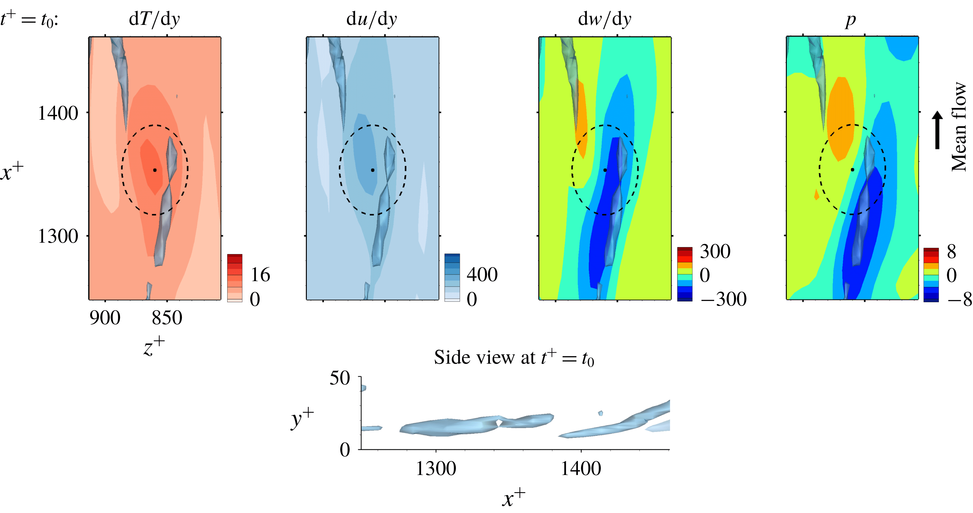
The first example fields yielding poor prediction. The point is on the local maximum error location. The vortices are visualized with
 $\unicode[STIX]{x1D706}_{2}=-0.05$
.

The second example fields yielding accurate prediction. The point is on the local maximum location. The vortices are visualized with
 $\unicode[STIX]{x1D706}_{2}=-0.05$
.
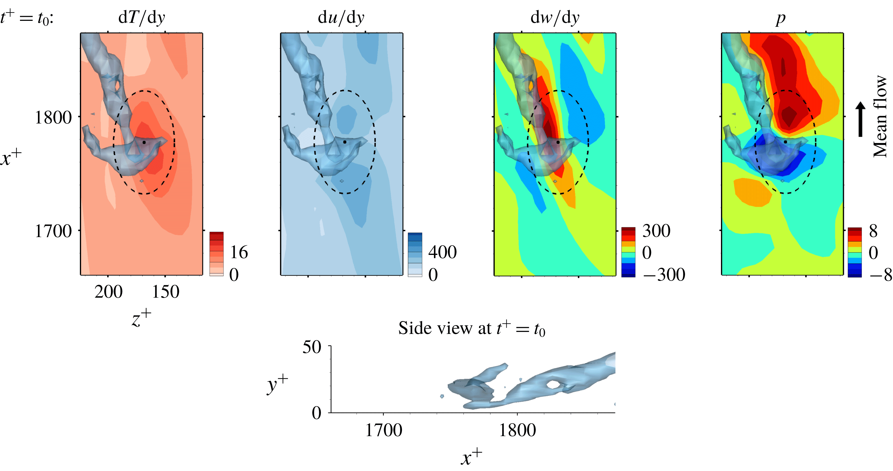
The second example fields yielding poor prediction. The point is on the local maximum error location. The vortices are visualized with
 $\unicode[STIX]{x1D706}_{2}=-0.1$
.

The near-wall streamwise vortices induce a sweeping motion that pushes fluid carrying high momentum and high temperature towards the wall so that both the streamwise wall shear and the heat flux are enhanced. Then, the streamwise vorticity and pressure show high correlation as shown in figure 11 for which deep learning predicts very well. However, for the similar situation shown in figure 12, where the streamwise vorticity is highly correlated with the wall pressure, the prediction by deep learning is poor. The difference between these two cases can be found in the side view of the near-wall vortices shown in figures 11 and 12; the vortex in figure 11 is slightly slanted away from the wall, whereas the vortex in figure 12 is slanted towards the wall at the point of interest. The former case is more frequently observed than the latter case; thus the latter case is not well learned by the network due to the small number of samples in training data, leading to poor prediction. The instantaneous distributions of the input fields alone cannot distinguish well between the two cases, but a consideration of temporal behaviour can help to identify the difference. For the well-predicted case, the strength of the vorticity and pressure increases with time, while the reduction of the vorticity and pressure over time is noticeable in two snapshots captured at different times, as shown in figure 12.
The second group of examples is the case where the wall vorticity distribution is quite different from the pressure distribution. Figure 13 demonstrates the case where a near-wall vortex strongly tilted towards the spanwise direction causes such a situation. Despite the dissimilarity between the shear stress and the heat flux at the prediction time, deep learning captures the difference well. On the other hand, the case shown in figure 14, where the wall vorticity distribution is too complex and there is a large pressure gradient, is not well predicted by deep learning. Here, again, the difference between the two cases lies in the temporal behaviour: the wall vorticity and pressure increase with time at the point of interest, leading to an increase in the heat flux in the former case (figure 13), whereas the pressure gradient decreases very quickly with time, leading to a quick increase in the shear stress in the latter case (figure 14).
Deep learning results considering the pressure field
 $p^{\ast }$
at an earlier time by
 $\unicode[STIX]{x0394}t^{+}$
as an extra input for prediction of the local heat flux. Training was performed using data of
 $Re_{\unicode[STIX]{x1D70F}}=180$
, and tests were carried out at
 $Re_{\unicode[STIX]{x1D70F}}=180$
and 540.

Through these observations, we can conjecture that the accurately predicted cases are found in the regions where the vorticity and pressure increase with time and the heat flux is enhanced, and that the inaccurately predicted cases are observed in the regions where the vorticity and pressure decrease with time. In particular, the sharp decrease in the streamwise gradient of pressure is responsible for poor prediction. To improve the performance of deep learning, the temporal information can be considered in the input. We carried out additional deep learning taking into account the pressure at a little earlier time than the present time as an extra input. We varied the time interval (
 $\unicode[STIX]{x0394}t^{+}$
) between the original inputs and the additional input from 0.9 to 7.2 in wall time units. As shown in table 3, the mean and r.m.s. values of all the deep learning models are very similar to those of the DNS. Although the models considering the temporal information (
 $p^{\ast }$
) show similar correlation coefficients between the prediction and the DNS, the model at
 $\unicode[STIX]{x0394}t^{+}=7.2$
is the best among the implemented models in the prediction of the local heat flux, with a correlation of approximately 0.983, which is slightly higher than the case without considering the temporal information. For the test at
 $Re_{\unicode[STIX]{x1D70F}}=540$
, which is not trained, the correlation coefficient between the prediction and the DNS is approximately 0.979. It is confirmed that pressure information for just one extra time step can improve the prediction accuracy. The results imply that information from several time steps of all variables might enhance the prediction of the local heat flux. Then, three-dimensional convolutional neural networks with time-directional convolution or recurrent neural networks, which use sequential information as inputs, might work as well. It will be more effective to apply the Lagrangian perspective considering the mean propagation speed of the input information when using those methods. However, the current deep learning, which does not consider time-dependent information, shows sufficiently reliable prediction accuracy.
3.3 Gradient analysis of the trained network
In the previous section, we have shown that the local heat flux can be well predicted on the basis of the nearby distributions of the wall-shear stresses and pressure by deep learning, which connects the input and the output through a nonlinear explicit relationship. Although the number of weights involved in the trained network is huge, an investigation of the relationship between the input and output might provide some clues to a better understanding of the near-wall physics of turbulence. In this section, we analyse the relationship between the wall-shear stresses, pressure and heat flux using the gradient map. First, we focus on the parts of the inputs that are important for the local heat flux prediction. The sensitivity analysis was performed by Simonyan, Vedaldi & Zisserman (Reference Simonyan, Vedaldi and Zisserman2013) to visualize the class saliency map for image classification problems. For regression problems, the sensitivity can be defined as the gradient of the output with respect to the input maps at each pixel, indicating how much the change in each input pixel value affects the output:
 $$\begin{eqnarray}S_{i,j}=\frac{\unicode[STIX]{x2202}O(I_{i,j})}{\unicode[STIX]{x2202}I_{i,j}}.\end{eqnarray}$$
Here
 $S_{i,j}$
,
 $I_{i,j}$
and
 $O(I_{i,j})$
are respectively the gradient maps, the input kernel maps over
 $N_{x}\times N_{z}$
regions used for prediction of a single point value of heat flux, and the output, which represents the convolutional neural network; and
 $i$
and
 $j$
represent the pixel indices of the minimum input in the streamwise (
 $x$
) and spanwise (
 $z$
) directions, respectively. The position
 $i=0,j=0$
corresponds to the point of interest. If we approximate the network as a multiple linear regression model composed of the same number of weights as the pixels of the input, the gradient signifies the values of the weights multiplied by each pixel of input,
 $$\begin{eqnarray}S_{i,j}\approx w_{i,j}\quad \text{if }O(I_{i,j})\approx \sum w_{i,j}\,I_{i,j}+b,\end{eqnarray}$$
where
 $w_{i,j}$
and
 $b$
are the weights and bias of the multiple linear regression approximating the network.
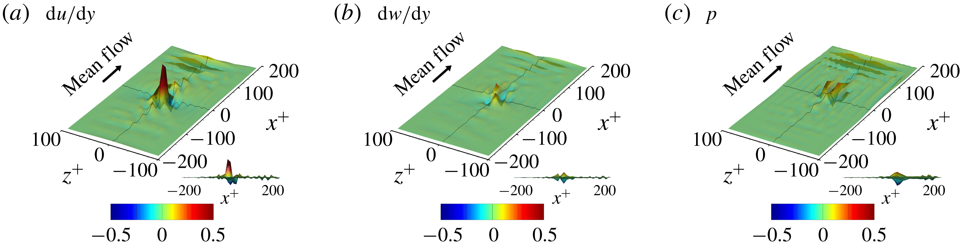
The gradient map obtained from an input kernel size dataset is quite different for each input dataset due to the nonlinear nature of the network and sometimes too noisy to allow any pattern to be recognized. The noise might originate from the training process under complicated situations where the relationship between the inputs and the output is not unique. In other words, it may be a kind of overfitting. However, the pixelwise average of the gradient maps over several input datasets shows a noticeable pattern regardless of the hyperparameters. Figure 15 shows the average gradient maps of the test datasets, which clearly demonstrate a non-negligible pattern near the point of interest. Therefore, it makes sense to investigate these patterns to understand the role of the nearby input data in determining the heat flux at the point of interest.
Average gradient maps of the optimal network. The black line is the centreline of each axis, and
 $(0,0)$
is the point of interest where the local heat flux is predicted. The side view is provided at the bottom right of each panel.
(a–c) Average and (d–f) r.m.s. of the noise-reduced gradient maps of the network using the large-size inputs.
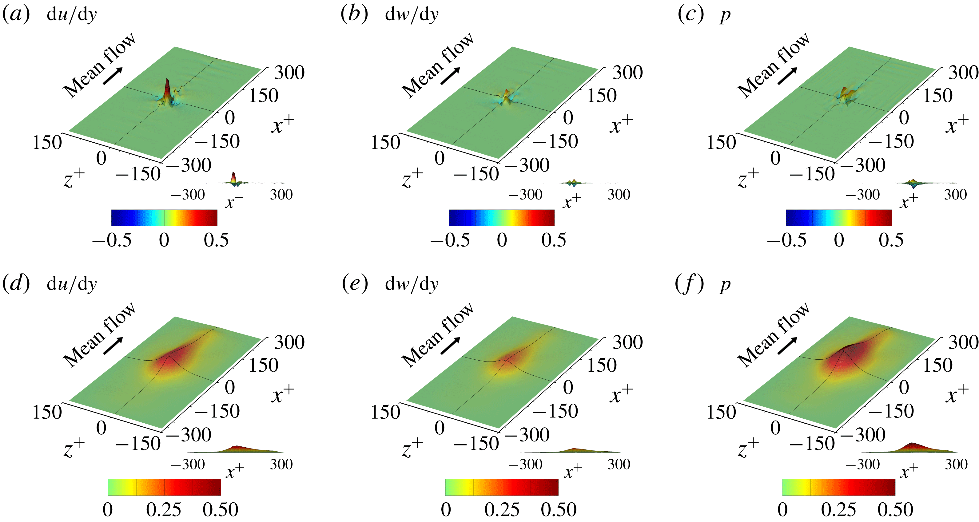
Before discussing the implications of the gradient map in detail, the quality of the gradient map needs to be refined. As shown in figure 15, wavy noise is observed in the downstream region in all gradient maps of the wall-shear stresses and pressure, and appears to be a numerical artifact. Upon investigation, we found that this phenomenon is related to the weights in the edge of the input image in the last layer. One way to resolve this is to apply stronger regularization to the weights towards the edge of the input image; however, this did not prove to be very successful. Another attempt to suppress this noise can be made by increasing the input kernel size, the region connected with a single point heat flux, because the noise is likely to come from the discontinuity of the weight distribution near the edges. We increased the input kernel size from
 $33\times 33$
to
 $49\times 49$
just for the purpose of the gradient analysis, to eventually suppress the noise significantly, as shown in figure 16.
In addition to the average, the r.m.s. of the fluctuations of the gradient maps is also shown in figure 16. The parts in which both the average and r.m.s. of the gradient are very small can be regarded as unnecessary regions for the prediction of the local heat flux. It appears that the regions
 $x^{+}<-150$
(upstream) or
 $|z^{+}|>100$
(spanwise sides) are unnecessary parts, while the downstream region up to
 $x^{+}=300$
is the necessary part. This implies that information located further in the downstream direction rather than the upstream direction is more critical in the prediction of the heat flux. However, the prediction accuracy is only slightly enhanced with an increase in the input kernel size as shown in the comparison between DL and DL3 in table 4, and thus increasing the input kernel size in the downstream direction is not expected to enhance the accuracy significantly. Besides, because the average and r.m.s. of the gradient maps are non-negligible only in the narrow neighbourhood of the point of interest, we can assume that the critical parts are very narrow in the context for good prediction.
Deep learning results for different combinations of the input fields. Input grid points (
 $N_{x}\times N_{z}$
) are increased from
 $33\times 33$
(DL) to
 $49\times 49$
(DL1, DL2, DL3) in order to reduce the noise of the average gradient maps.

In such narrow parts of the average gradient map of the trained network, strong gradient values in the specific distribution are observable regardless of the hyperparameters, implying some physical meaning. For the comparative analysis with the present model (DL3), two more deep learning procedures with a different combination of the inputs, such as a model using the shear stress and vorticity as the inputs (DL1) and another model using the shear stress and pressure as the inputs (DL2), were carried out (table 4). In addition to these three cases, other deep learning procedures including models using only one type of input and a model not using the shear stress as input were performed and the results are provided in table 5 in appendix A. Because the prediction accuracy of DL1, DL2 and DL3 is much higher than that of the other cases, we consider only these cases here, except to mention that it is interesting that the model using only the vorticity and pressure without the information of momentum streaks can predict thermal streaks well and produces a correlation coefficient of 0.959 with DNS data. While the accuracy of DL1 and DL2 is similar, the prediction of DL3 is slightly more accurate than those of DL1 and DL2. Also, for observing the linear relation between the input and output, a multiple linear regression (MLinear1) using the same inputs as DL3 was carried out. The accuracy of MLinear1 is almost the same as that of MLinear (table 2). Here, L1 regularization was used to prevent noise in the gradient map of MLinear1. For MLinear1, the r.m.s. values of the fluctuations of gradient maps are all zero simply because
 $S_{i,j}$
becomes equal to
 $w_{i,j}$
. The magnified views near the point of interest of the average gradient maps of DL1, DL2, DL3 and MLinear1 are presented in figures 17, 18, 19 and 20, respectively.
Magnified view of the average gradient maps of DL1 in which the inputs are the shear stress and vorticity.
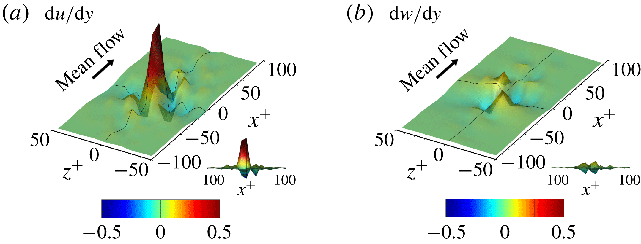
Magnified view of the average gradient maps of DL2 in which the inputs are the shear stress and pressure.

Magnified view of the average gradient maps of DL3 in which the inputs are the shear stress, vorticity and pressure.

Magnified view of the gradient maps of MLinear1 in which the inputs are the shear stress, vorticity and pressure.
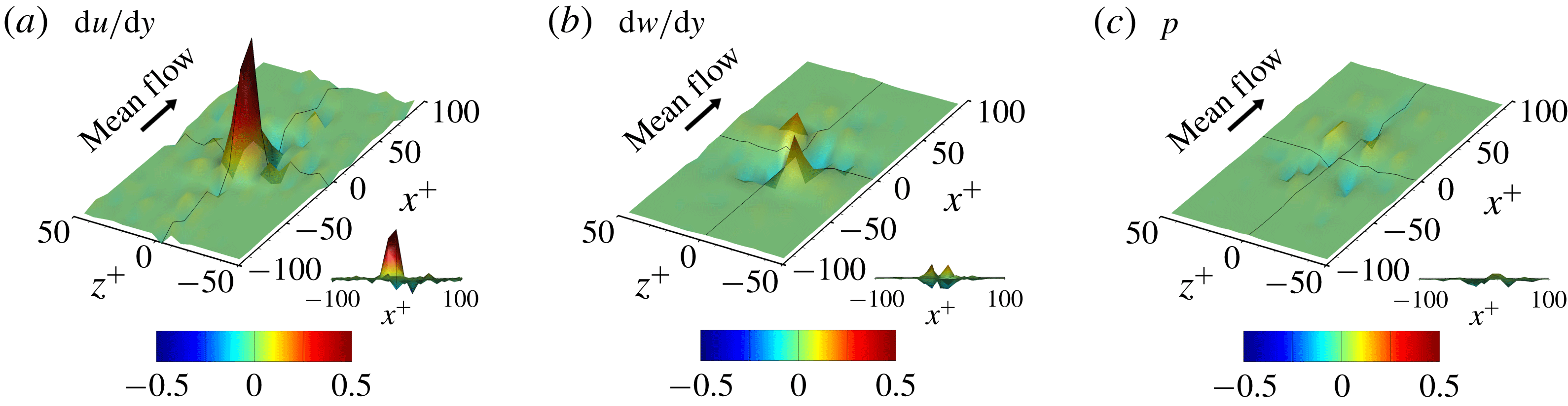
For all cases, the average gradient maps show that the streamwise wall-shear stress is the most influential in the determination of the heat flux, as expected, and the strong positive peak is found to be slightly shifted towards upstream of the point of interest (
 $x^{+}<0$
). A negative gradient is commonly observed in the spanwise sides and downstream of the strong positive peak in all cases. For DL1, DL3 and MLinear1, the average gradient maps of the streamwise vorticity are large on both sides downstream (
 $x^{+}>0,|z^{+}|>0$
), which is consistent with the report for the relationship between the shear stress and the streamwise vortices (Kravchenko et al.
Reference Kravchenko, Choi and Moin1993). In the first quadrant of the input map (
 $x^{+}>0,z^{+}>0$
), the gradient of the heat flux with respect to the vorticity is positive, whereas the gradient is negative in the fourth quadrant (
 $x^{+}>0,z^{+}<0$
), due to the skew symmetricity (
 $S_{i,j}=-S_{i,-j}$
). On the other hand, in the second (
 $x^{+}<0,z^{+}>0$
) and third (
 $x^{+}<0,z^{+}<0$
) quadrants, similar correlations exist with signs opposite to the first and fourth one, respectively. This implies that the sweep motions downstream or vortices crossing from the third to the first or from the second to the fourth quadrant can strongly enhance the local heat flux even if the shear stress is low. The average gradient maps of streamwise shear stress and vorticity in all cases, including the linear model, show similar distributions. However, this does not necessarily mean that the linear and DL models act similarly. It is noteworthy that the prediction accuracy of DL1 (
 $R=0.977$
), which uses only the wall-shear stresses as input, is higher than that of MLinear1 (
 $R=0.964$
), although MLinear1 uses more input information. Furthermore, the DL model produces meaningful distributions of the r.m.s. of the fluctuations of gradient maps, which is absent in the linear model. This input-dependent property of DL is a major difference between the nonlinear mapping and linear one, which somehow produces a better correlation than the linear network.
For DL2, in which the streamwise shear stress and pressure are used as input, the average gradient map of the pressure upstream is negatively correlated with the heat flux at the point of interest, whereas that downstream is positively correlated while maintaining the symmetry in the spanwise direction (
 $S_{i,j}=S_{i,-j}$
). This indicates that the pressure gradient in the streamwise direction at the point of interest indeed positively influences the heat flux, which is consistent with the results of Abe & Antonia (Reference Abe and Antonia2009). Comparing DL2 and DL3 (figures 18 and 19), however, we can notice that the average gradient maps of the pressure are significantly different. This difference is obviously caused by the inclusion of the vorticity in the input for DL3, suggesting that there might be some correlation between the vorticity and the pressure fields. Kim (Reference Kim1989) reported that the large-negative-pressure parts strongly correspond to the large-streamwise-vorticity parts, and the vorticity is similar to the spanwise pressure gradient. For DL3 and MLinear1, which use the same input information, a remarkable difference is observed in the average gradient map of the pressure, as shown in figures 19(c) and 20(c), while the average gradient maps of the wall-shear stresses are similar. This indicates that pressure influences the heat flux through the nonlinear mapping when the entire wall information including shear stresses and pressure is used as input. This explains why the linear network performs relatively well, but the nonlinear DL produces a better result by capturing the nonlinear relation between the input and output.
Additional deep learning procedures to quantitatively investigate the dependence between the wall variables are carried out, and the results are presented in table 6 in appendix A. Prediction of the vorticity based on the nearby pressure information is very accurate with
 $R=0.974$
, but the inverse prediction of the pressure based on the vorticity is not so accurate with
 $R=0.881$
. This suggests that pressure has more information than the vorticity and that the wall pressure cannot be predicted on the basis of wall information alone.
In fact, the average gradient maps, which we have discussed above, contain more information on the gradient of the input of low magnitude, because the input field of low magnitude is more frequently found. Therefore, the average gradient map might be biased to the input of low magnitude. However, we are more interested in the behaviour of the input fields that cause a strong heat flux. In order to focus on the gradient maps of large-magnitude inputs, here, we observe the change in output caused by the relative change in the input magnitude. In other words, relative gradient maps to observe the output change when the value on each pixel of the input maps is multiplied by a factor
 $f$
that is almost equal to 1 were defined:
 $$\begin{eqnarray}RS_{i,j}=\frac{O(f\,I_{i,j})-O(I_{i,j})}{\text{sign}(I_{i,j})(f-1)},\end{eqnarray}$$
where
 $RS_{i,j}$
are the relative gradient maps, and
 $f$
is 1.1. In the operation of
 $f\,I_{i,j}$
,
 $f$
is multiplied to an input variable at the
 $i,j$
position only. The
 $RS_{i,j}$
value is similar to
 $S_{i,j}$
, but it emphasizes large-amplitude input. Figure 21 shows the average relative gradient maps for DL3, which is consistent with the previous average gradient maps (figure 19), indicating that the average gradient maps are valid for the overall range of the inputs in our problem. The only noticeable difference is found in the amplitude of the average gradient maps such that the peak value of the gradient map of the shear stress decreases. The decrease implies that, as the input values are large, the linear relationship between the shear stress and the heat flux becomes weak. There is a similar quantity that reflects the magnitude of the input to the gradients such as
 $|I_{i,j}|\,S_{i,j}$
, which can intuitively extract the relations between turbulent structures and predicted heat fluxes. We also confirmed that the average result of this quantity is similar to the relative gradient map.
Magnified view of the relative average gradient maps of DL3.
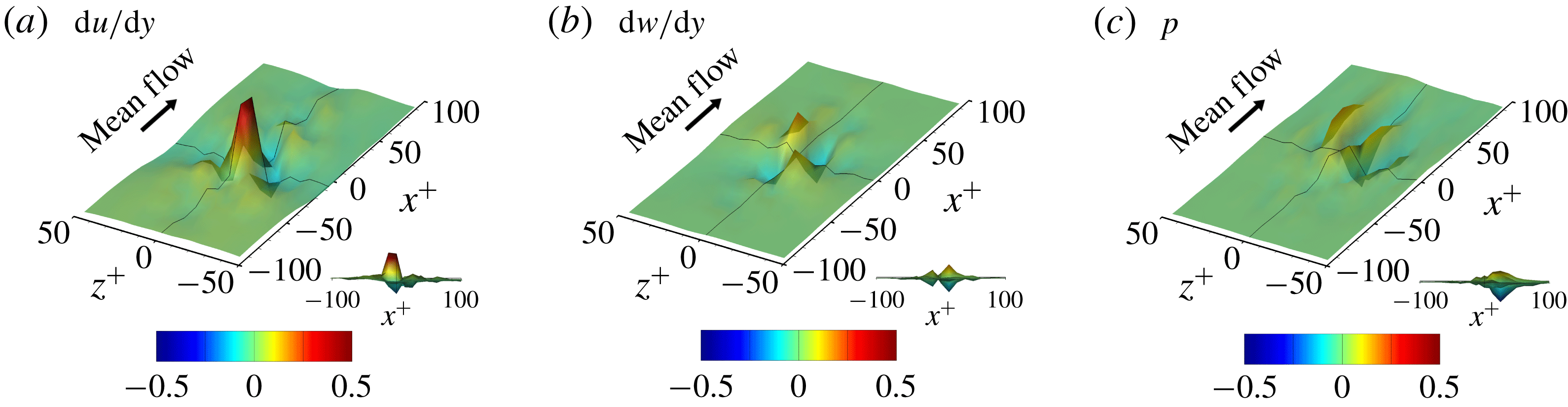
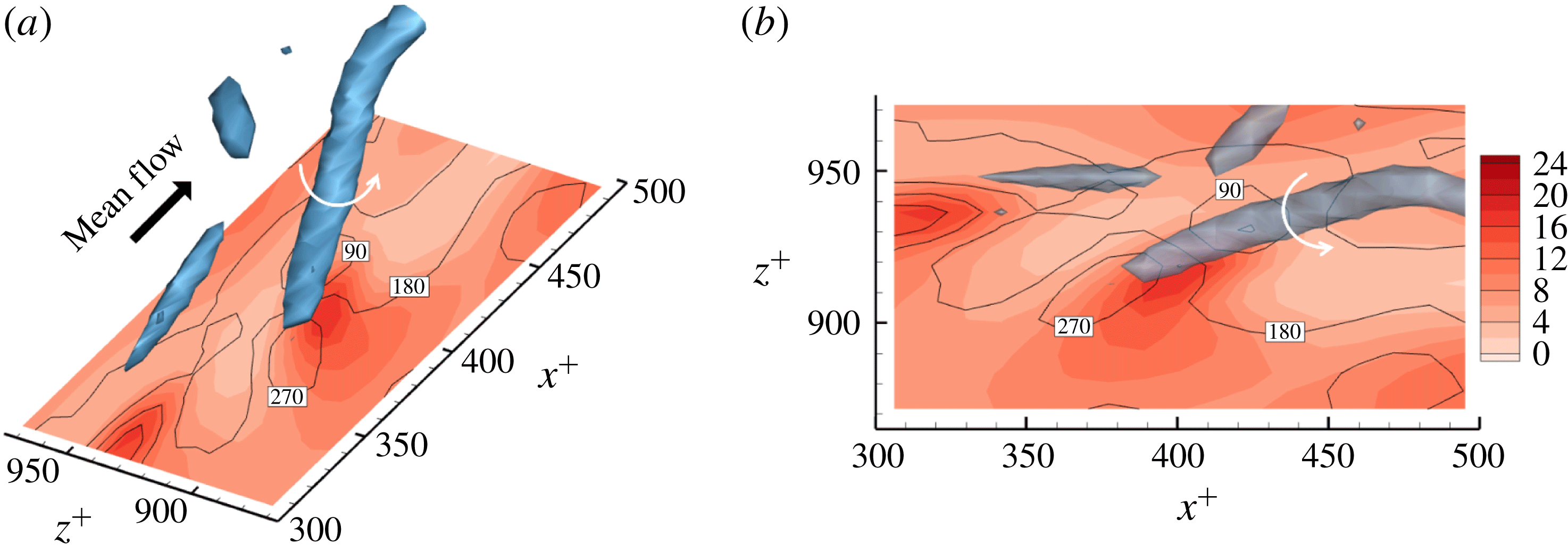
Figure 22 demonstrates a good example that clearly shows the relationship between the local heat flux and the nearby vorticity on the wall. There is a strong streamwise vortex that is slightly tilted anticlockwise in the horizontal (
 $x$
–
 $z$
) plane. Then, a strong and positive streamwise vorticity occurs on the wall and is tilted, and high heat transfer is observed along this vortex. The local maximum value is approximately three times higher than the average heat transfer rate, while the streamwise shear stress value near the maximum position is approximately the average shear stress. This situation results in a large contribution to the positive values at the first and third quadrants in figures 17(b), 19(b), 20(b) and 21(b). Conversely, the negative values in the second and fourth quadrants are obviously caused by the vortex tilted clockwise on the horizontal (
 $x$
–
 $z$
) plane.
Representative case with high heat transfer at
 $Re_{\unicode[STIX]{x1D70F}}=180$
. Panel (b) is the top view of panel (a). Isocontours are used for the heat flux, the lines are used for the streamwise shear stress, and
 $\unicode[STIX]{x1D706}_{2}=-0.1$
. The local maximum value of the heat flux is approximately three times higher than the average heat flux, while the local shear stress value at the same location is similar to the mean shear stress.
In addition to the gradient, the second-order derivatives can be used to identify the local complexity of a function (Wahba Reference Wahba1990). However, in our applications of deep neural networks to represent the relationships between turbulence data, when the network is deeper, the second-order gradients typically increase significantly without a meaningful increase in the prediction accuracy. The increase in the second-order gradients results in rather noisy individual gradient maps. In other words, the overfitting, which does not affect the prediction accuracy, makes gradient analysis difficult even when the number of training datasets is large enough. In order to analyse individual cases through the gradient maps, it is critical to minimize such overfitting. There are several possible methods to prevent overfitting, such as to make the network relatively shallow, to strengthen the regularization, and to directly add the average of the second derivatives to the loss function as a constraint (this greatly increases the computation load and memory). Those are not attempted in the present study. In short, the second-order derivatives are so sensitive to the hyperparameters that investigation of them was not so informative, and it is crucial that they be reduced for a deeper gradient analysis.
Finally, we briefly mention what we can learn from an analysis of the weights of the trained network. In general, it is almost impossible to completely understand the role of all weights in a multilayered network. However, because we are adopting a convolution network, we might be able to grasp the roles of some weights in successful learning by investigating the distribution of the weights. Here, we focus on the first convolution layer, which is directly applied to the input fields to predict the target output. In order to quantify the importance of each kernel in the convolution layer, we carried out a kernel sensitivity analysis. All the weights of a specific kernel were deliberately set to zero while keeping the weights of other kernels as the trained networks, and the resulting change in the prediction accuracy in terms of the correlation coefficient
 $R$
was monitored. The changes are generally proportional to the magnitude of the weights in the kernels, but not always, because of the scale factor in the batch normalization.
Kernel sensitivity analysis for quantifying the importance of kernels. (a) Weight distribution of the kernels in the first convolution layer; (b) changes in
 $R$
; and (c) magnified view of prominent kernels that play an important role in the prediction of heat flux.

Figure 23(a,b) shows the
 $3\times 3$
weight distribution of the kernels in the first convolution layer of the trained network and the corresponding response of the kernel sensitivity test in terms of the change in
 $R$
for the case DL3, respectively. Here, the first, second and third input maps correspond to the shear stress, vorticity and pressure, respectively, and the number of output feature maps in the first layer is 24. The orientation of the
 $3\times 3$
weights is such that the horizontal and vertical directions denote the streamwise and spanwise directions, respectively. Almost all the kernels at least slightly influence the prediction performance. In particular, among the kernels of the first input map, the kernels of the fifth and twentieth output feature maps play the most important roles. The weight distribution of the corresponding kernels shown in figure 23(c) indicates that the dominant weights of the fifth feature map are all negative while those of the twentieth map are positive. This implies that each kernel detects the low-speed and high-speed streaks of the shear stress, which are characterized by negative and positive values, respectively, through the action of the nonlinear activation function given in (2.7). Because these streaks influence the heat flux through different mechanisms, the network needs to differentiate these in the layer of feature map extraction.
An investigation of the tenth feature maps of the vorticity and pressure input maps shown in figure 23(c) revealed that the feature map of the vorticity extracts the vorticity value itself while that of the pressure extracts the spanwise gradient of the pressure. This indicates that both maps detect the presence of a near-wall vortex because the vorticity and spanwise gradient of the pressure are highly and negatively correlated. When one signal is weaker than the other, these kernels capture the difference between them. This result is closely related to the nonlinear effect reflected on the average gradient maps of the pressure, shown by the difference between figures 19(c) and 20(c). It can be seen that the weight distribution of the twenty-third feature maps shown in figure 23(c) is opposite in sign to the tenth maps for both the vorticity and pressure inputs. This preserves the reflectional symmetry so that the streamwise vortex rotating either positively or negatively about the streamwise direction can be detected equally. There are other important kernels, but it is not easy to understand their roles in the physical sense. Understanding the role of kernels in the deeper layer and the connections between the layers is even harder. With the development of more sophisticated methods for analysing deep learning such as visualizations using deconvolution (Zeiler & Fergus Reference Zeiler and Fergus2014) and layerwise relevance propagation (Bach et al. Reference Bach, Binder, Montavon, Klauschen, Müller and Samek2015), we might have more opportunities to further understand the physics of turbulence.
3.4 Application to low-resolution data
We presented the model for predicting turbulent heat transfer from the spatial information of shear stresses and pressure on the wall. We showed that the heat transfer could be well predicted by the nonlinear network if accurate wall-shear stresses and pressure, which are provided by DNS, are used as input. In more practical applications, such as LES or RANS, however, such high-quality input data are not available. Therefore, the DL framework that we developed could not be directly applied to LES or RANS. In this section, we investigate the possibility that our DL could be utilized in LES or RANS.
We carried out a new deep learning procedure, DL-RV, for the prediction of the well-resolved turbulent heat transfer using poorly resolved wall-shear stresses and pressure. This procedure is similar to the super-resolution reconstruction of turbulence (Fukami, Fukagata & Taira Reference Fukami, Fukagata and Taira2019), in which they had the same input variables as the output variable. Our poorly resolved input data were obtained by truncation of the DNS data in the horizontal wavenumber domain, and the number of grids in the physical domain was set equal to the full resolution through spectral interpolation. Thus, the number of input kernel grids (
 $N_{x}\times N_{z}$
) and the grid interval in wall coordinates (
 $\unicode[STIX]{x0394}x^{+},\unicode[STIX]{x0394}z^{+}$
) are the same as those in table 2. The target output is the accurate heat flux data obtained from DNS. Various wave resolutions between
 $128\times 128$
(full) and
 $16\times 16$
were considered as the training input data. The DL network was trained using the data of those resolutions altogether.
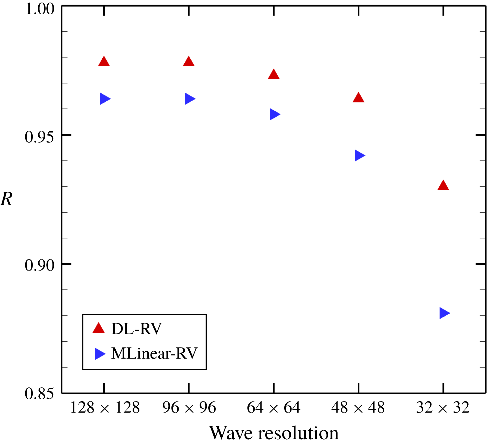
The prediction results of the trained DL-RV in terms of the correlation coefficient
 $R$
are shown in figure 24. For the purpose of comparison, a multiple linear regression, MLinear-RV, was trained using the same training data as that of DL-RV. As expected, as the resolution decreases, the accuracy of DL-RV and MLinear-RV decreases naturally due to the lack of input information. The prediction accuracy of MLinear-RV decreases considerably with a decrease in the input wave resolution, while that of DL-RV drops relatively slowly. Even at the resolution of
 $32\times 32$
, the value of
 $R$
for DL-RV is around 0.93, which is not bad given that the input data were filtered over four grids in each direction. This implies that the relationship between the poorly resolved inputs and the fully resolved heat flux is strongly nonlinear. The fields predicted by DL-RV and MLinear-RV when the wave resolution of the input is
 $32\times 32$
are illustrated in figure 25. Although the locally high heat flux is not completely represented as compared to the DNS data, the overall trend is well captured by DL-RV, while in the prediction by MLinear-RV, the small-scale behaviours are hardly found. These results clearly indicate that our DL model has the potential to be applied to low-resolution simulations such as RANS or LES.
Prediction accuracy with change in input resolution at
 $Re_{\unicode[STIX]{x1D70F}}=180$
. For all cases, the turbulent heat transfer of training and testing data was a fully resolved one.
Predicted turbulent heat transfer from the low-resolution input fields using DL-RV. (a) The DNS field and the low-resolution input field; and (b) the DNS heat flux field, and the predicted heat flux fields by DL-RV and MLinear-RV.

We have not trained our DL network using RANS or LES data. However, we have shown that the poorly resolved input can yield accurate output if the network is properly trained. For successful training, one needs pairs of RANS or LES input data and accurate output data, which are usually not available. As a remedy to this problem, unsupervised learning could be considered. Kim & Lee (Reference Kim and Lee2019) showed that it is possible to learn a similarity between simulations with different Reynolds numbers through unsupervised learning of turbulence. Likewise, connecting data from low-resolution and high-resolution simulations would be possible.
4 Conclusions
The current study proposes a CNN model that can predict the wall-normal heat flux on the basis of only wall information, including the streamwise wall-shear stress, spanwise wall-shear stress (streamwise vorticity) and pressure fluctuations. In order to collect data used for the training of the CNN, DNS of turbulent channel flow with a passive temperature field at three frictional Reynolds numbers (
 $180$
,
 $360$
and
 $540$
) were conducted. A total of
 $6400$
uncorrelated fields at
 $Re_{\unicode[STIX]{x1D70F}}=180$
and
 $50$
extra uncorrelated fields were collected as training and test data, respectively. In addition, the 50 fields obtained at
 $Re_{\unicode[STIX]{x1D70F}}=360$
and
 $540$
were collected only for test data. Several deep learning procedures were performed, tested and analysed using the given data.
In order to predict a field (
 $192\times 192$
) of the heat flux quickly, we used only convolution layers without zero padding. We constructed an architecture such that the output size can be changed depending on the change in the input size without any overlapped calculation. A single point of the output is connected with only small regions (input kernel size,
 $N_{x}\times N_{z}$
) of the input, even if the input size is bigger than
 $N_{x}\times N_{z}$
. During training, we used the biggest size input (
 $(191+N_{x})\times (191+N_{z})$
), which produces a similar effect to using a large batch size and thus stably and quickly learns sufficient training data on the network. The constructed network was trained using ADAM, and the grid searching method was performed to optimize the depth and width of the CNN. The resulting optimal CNN architecture consists of nine
 $3\times 3$
convolution layers, 24 feature maps in each convolution layer, and one
 $15\times 15$
convolution layer.
The prediction accuracy of the optimized model is quantified via comparison of several statistics of the heat flux against the DNS, such as mean, r.m.s., correlation coefficient (
 $R$
), p.d.f. and high-order moments. A simple linear regression model and a multiple linear regression model were considered for performance comparison. Test results show that, at
 $Re_{\unicode[STIX]{x1D70F}}=180$
, all the mean values of prediction are very similar to the DNS values, whereas the r.m.s. values predicted by deep learning and multiple linear regression are much closer to the DNS values than those predicted by the simple linear regression. Further,
 $1-R~(=0.02)$
of the optimal CNN is approximately one-fifth of
 $1-R~(=0.10)$
of the linear regression and half of
 $1-R~(=0.036)$
of the multiple linear regression. The p.d.f. and high-order moments of the optimal model also agree well with the DNS, confirming that deep learning can predict turbulent heat transfer considerably well. For the tests at
 $Re_{\unicode[STIX]{x1D70F}}=360$
and
 $540$
, the network trained at
 $Re_{\unicode[STIX]{x1D70F}}=180$
yielded a predictive performance similar to that of the trained
 $Re_{\unicode[STIX]{x1D70F}}$
. These results indicate that the relationship between the heat flux and the inputs including shear stresses and pressure is almost independent of the frictional Reynolds number within the tested range. Locally poor prediction was observed in some regions of the high heat flux, and an investigation of these regions revealed that an often large streamwise pressure gradient at an earlier time than the prediction time was identified as being responsible for the poor prediction.
In order to understand the physics associated with the local heat flux, we observed the gradient maps of the trained optimized network. The average and r.m.s. of the gradient maps were calculated, and the results reveal which parts of the input fields are critical for the local heat flux prediction. Both average and r.m.s. are very small in the region beyond 150 wall units in the upstream direction and in the region further than 100 in the spanwise direction, indicating that the information there is almost unnecessary for the prediction. In contrast, there are quite large r.m.s. values even up to 300 in the downstream direction. In particular, the average gradient maps near the point of interest show a similar trend regardless of the hyperparameters. For the shear stress, the average gradient map shows the strongest peak near the point of interest, a little bias towards the upstream direction. For the vorticity, the average gradient map is strong on both sides downstream, and they have opposite signs. Further, the map is strong on both sides upstream, and their signs are opposite to the downstream signs. This result implies that either when the vortex pair is downstream, or when a vortex crosses diagonally at the point of interest, the local heat flux can be enhanced. For the pressure, the average gradient map is biased towards the downstream direction due to the strong correlation with the vorticity, and it is observed that the trained network somehow captures the difference between them. Also, a noticeable difference is observed in the pressure maps of the DL and linear models, indicating that the linear model could not utilize the pressure information for prediction because of the nonlinear relationship. In short, we identified the spatial relationship between the local heat flux and inputs, which is nonlinear, through the analysis of the trained DL models.
For a practical application such as turbulence modelling, we carried out DL using various resolution input data as the training data. As a result, the DL model is less sensitive to the input resolution, indicating the possibility that our model could be a good heat flux model in turbulence simulation. There are some remaining issues, such as whether the trained model works well in modelled simulations like RANS or LES. For successful training, RANS input and accurate output should be provided. We expect that ‘unsupervised learning’, which can connect the low-resolution and high-resolution simulations, would be a key for it. This certainly suggests a future research direction.
In summary, we have proved our hypothesis in a current application of deep learning, namely, that the heat flux field, which is one of the near-wall turbulence fields, can be accurately predicted on the basis of only wall information, such as the shear stress and pressure. This clearly indicates that the wall information of the stresses and pressure is indeed sufficient to capture the near-wall physical process responsible for the determination of the heat flux. We have also shown that an investigation of the trained network structure can reveal the hidden physics of the near-wall turbulence. This is promising and encourages wider applications of machine learning to various turbulence phenomena for a better understanding of fundamental physics as well as for practical applications. Our code and the relevant datasets will be released as an open-source upon publication. Detailed information is given in appendix B.
Acknowledgements
This work was supported by the National Research Foundation of Korea (NRF) grant funded by the Korea government (MSIP) (2017R1E1A1A03070282).
Appendix A. Additional deep learning
Several deep learning procedures for different choices of input and output were carried out for the purpose of quantifying the dependence of the difference in prediction accuracy on the change of input and confirming the dependence between the input variables. Although the input and output changes require a new optimization process of the network, under the assumption that the difference will not be large, we used the same size of the input images
 $(49\times 49)$
and the same structure of the network as in DL3, which is composed of nine
 $3\times 3$
convolution layers, 24 feature maps in each convolution layer, and one
 $31\times 31$
convolution layer. The network was trained for 2000 epochs using 6400 original training fields with mirror-imaged ones, and the learning rate was reduced to
 $1/5$
per 400 epochs.
Deep learning results for various combinations of input fields for the local heat flux prediction. Training was carried out using data of
 $Re_{\unicode[STIX]{x1D70F}}=180$
, but tests were performed at
 $Re_{\unicode[STIX]{x1D70F}}=180$
and 540.
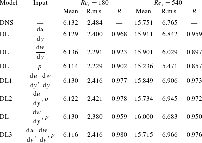
Deep learning results for various choices of input and output fields.
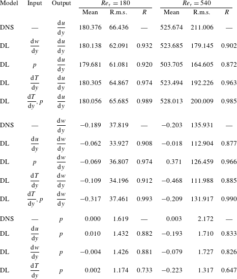
The results quantifying the prediction accuracy of deep learning for different combinations of input fields are given in table 5, including DL1, DL2 and DL3. All the mean values of the prediction show no large difference compared to the DNS. Interestingly, when the streamwise shear stress is not used as a part of the input, the local heat flux can be predicted relatively well on the basis of the pressure and vorticity information together, but not on the basis of one of these alone. The performance difference is more pronounced at
 $Re_{\unicode[STIX]{x1D70F}}=540$
.
In addition, the results of deep learning procedures that were carried out for quantification of the relationship between one field and other fields for various combinations of input and output are given in table 6. Here, for the test at a higher Reynolds number than the trained number, a similar scaling process as that applied to (3.2) and (3.3) was applied. As the preprocess of the input, the shear stresses and the heat flux except the pressure are scaled by the ratio of the frictional Reynolds numbers and the ratio of the Nusselt numbers, respectively. As the postprocess of the output, the predicted shear stresses except the pressure are scaled by the inverse ratio of the frictional Reynolds numbers.
The first thing to note in table 6 is the fact that the local vorticity can be predicted well on the basis of the nearby pressure information with a correlation of 0.974, whereas the inverse prediction of the pressure on the basis of the nearby vorticity information is much less accurate with
 $R=0.881$
. This indicates that pressure contains more information than vorticity, which is consistent with our observation that the average gradient maps of pressure for DL2 and DL3 (figures 18 and 19) are different. Besides, other deep learning procedures that predict wall information using the nearby heat flux were carried out, as given in table 6. Similarly to DL2, the network whose inputs are the heat flux and pressure can predict the local streamwise shear and vorticity very well (
 $R=0.989$
and
 $R=993$
, respectively), indicating that the dissimilarity between the shear and the heat flux is strongly related to pressure, as reported by Abe & Antonia (Reference Abe and Antonia2009). Finally, the predictions of pressure based on the shear stress, vorticity and heat flux are all poor. This indicates that, for the prediction of pressure, which is a global quantity, the wall information of stress or heat flux is not enough. For all cases, the performance differences are more pronounced in the test at
 $Re_{\unicode[STIX]{x1D70F}}=540$
.
Appendix B. Code release as open source
Our code and the relevant datasets are released as open source. We created a public repository, https://github.com/junhyuk6/THT-CNN, which will host the code and data upon publication of our paper.



