1 Introduction
The need to control (reduce) jet noise is most pressing for the take-off stages of aircraft operation and it is important to understand the influence of forward flight on jet noise generation mechanisms. Early experimental research showed that jets in flight conditions are quieter compared to the same jets in a static environment (see e.g. Crighton, Ffowcs Williams & Cheeseman Reference Crighton, Ffowcs Williams and Cheeseman1977; Tanna & Morris Reference Tanna and Morris1977) and a number of theoretical and semi-empirical corrections to account for the flight conditions have been derived (cf. Michalke & Michel Reference Michalke and Michel1979a
,Reference Michalke and Michel
b
). These corrections can be used to obtain reasonable predictions of the noise levels, and it has been shown that the pressure power spectral density (PSD) for a co-flowing jet at
 $90^{\circ }$
should scale with
 $(u_{CL}-u_{co})^{5}u_{CL}^{3}$
, where
 $u_{CL}$
and
 $u_{co}$
are the jet exit centreline and co-flow velocities, respectively. Thus the velocity scaling shows a considerable dependence on the co-flow velocity.
However, it is not clear whether this velocity scaling applies only to the overall PSD or whether it also applies to different frequency ranges and individual azimuthal modes of the jet noise. Overcoming this lack of detailed understanding has become even more important in current jet noise research, where the error bars in measurements of jet noise have become smaller and high-quality simulations are able to match experimental data within 2–3 dB (see e.g. Bogey, Marsden & Bailly Reference Bogey, Marsden and Bailly2011). The lack of a fundamental understanding of the differences between noise sources in static and flight conditions is also a barrier when it comes to extrapolating the results of noise control strategies (such as microjets and/or chevrons) to flight conditions, as was clearly demonstrated in recent work by Shur, Spalart & Strelets (Reference Shur, Spalart and Strelets2010), in which the efficiency of a microjet noise reduction concept in static and flight conditions was examined.
Juvé, Sunyach & Comte-Bellot (Reference Juvé, Sunyach and Comte-Bellot1979) were one of the first to perform a modal decomposition (azimuthally) of the acoustic far field and found that, depending on the observation angle, different azimuthal modes dominated and showed a characteristic shape. In a more recent study by Kopiev et al. (Reference Kopiev, Chernyshev, Faranosov, Zaitsev and Belyaev2010), the azimuthal correlation of the far-field noise was investigated for unexcited and tone-excited jets. However, both studies only considered a single jet Mach number and therefore did not investigate the Mach-number scaling of the azimuthal modes. Cavalieri et al. (Reference Cavalieri, Jordan, Colonius and Gervais2012), however, did report the velocity dependence of the sound radiation for azimuthal modes
 $m=0$
, 1 and 2 for jet Mach numbers between 0.4 and 0.6 and found that, for a nozzle-diameter-based Strouhal number of 0.2, the velocity exponent depended strongly on observation angle, with values ranging from close to 8 at
 $20^{\circ }{-}30^{\circ }$
to around 7 at
 $90^{\circ }$
with respect to the axis. The velocity scaling of the azimuthal modes
 $m=1$
and 2 was found to be similar to the axisymmetric mode
 $m=0$
and the total for the overall sound pressure level. Although the study was limited to a fairly narrow Mach-number range, to Strouhal numbers and azimuthal modes up to unity and
 $m=2$
, respectively, due to the constraints of the experimental set-up, the results are relevant, as the most significant contribution of jet mixing noise is within this parameter space. However, this investigation did not include any effect of co-flow and the reported exponent appears to be contradicting other studies, such as those reported in Tam et al. (Reference Tam, Viswanathan, Ahuja and Panda2008), where an exponent of close to 8 was reported at
 $90^{\circ }$
, rising to even larger values at smaller angles relative to the downstream direction.
Therefore, to get further physical insight into the dominant jet noise generation mechanisms and velocity scalings for varying jet exit and co-flow velocities, it is desirable to obtain high-fidelity data of both the hydrodynamic and acoustic fields of the jet simultaneously. For the results to be reliable, however, it is important that the simulated jet captures all relevant mechanisms. It is well known that several different sources contribute to the overall sound radiation from subsonic jets: (i) large-scale structures mainly occurring close to the potential core region, (ii) breakdown of large-scale structures into fine-scale turbulence near the end of the potential core, (iii) fine-scale turbulence within the initial shear layers of fully turbulent jets, and (iv) trailing-edge noise resulting from the interaction between flow and the solid wall at the nozzle exit. Furthermore, the importance of the initial conditions on the jet development and noise has been well documented (Hussain & Zedan Reference Hussain and Zedan1978; Gutmark & Ho Reference Gutmark and Ho1983; Zaman Reference Zaman1985; Raman, Zaman & Rice Reference Raman, Zaman and Rice1989; Bogey & Bailly Reference Bogey and Bailly2010). Thus, to capture the above-mentioned noise generation mechanisms and to consider realistic initial conditions for the jet, simulations in which the nozzle is included and the flow exiting the nozzle is fully turbulent are required. This configuration was considered by Sandberg, Suponitsky & Sandham (Reference Sandberg, Suponitsky and Sandham2012), who simulated turbulent flow exiting a pipe into a laminar co-flow for three subsonic jet Mach numbers and varying co-flows, using direct numerical simulation (DNS) to eliminate uncertainties associated with turbulence modelling.
However, subsequent studies of these data using phased-array techniques found that the original DNS were contaminated by high levels of internal noise, generated within the pipe, and that it was difficult to extract the jet mixing noise, in particular for the axisymmetric mode (Sandberg & Tester Reference Sandberg and Tester2012; Tester & Sandberg Reference Tester and Sandberg2013). Therefore, a new set of DNS were performed with several vital modifications, most noteworthy an explicit elimination of fluctuations in the axisymmetric mode of the turbulent inflow generation, and the use of an acoustic liner boundary condition for the inside of the pipe. In a precursor study, an acoustic liner model based on an impedance boundary condition was shown to be effective at removing acoustic fluctuations within the pipe without affecting the turbulent flow field (Olivetti, Sandberg & Tester Reference Olivetti, Sandberg and Tester2015). The first analysis of the new DNS data has shown that the change in inflow boundary condition is largely responsible for reduction of internal noise of the axisymmetric mode, while the main role of the acoustic liner is the absorption of internal noise for higher azimuthal modes (Sandberg Reference Sandberg2014). The main focus of the current paper is on using a source breakdown technique, based on a phased-array approach, to establish the Mach-number scaling of individual azimuthal Fourier modes of far-field pressure for the jet mixing noise component of co-flowing jets for a jet Mach-number range from 0.4 to 0.8.
The paper is structured as follows. The definition of all the relevant non-dimensional parameters and the governing equations are given in § 2. The DNS code, the numerical set-up and the phased-array technique are presented in § 3. In § 4.1, the general features of the hydrodynamic and acoustic fields are discussed, followed by a presentation of the Mach-number scalings for the axisymmetric and higher azimuthal modes obtained using the phased-array technique in conjunction with a source breakdown in § 4.2. The paper concludes with a discussion of the most important results in § 5.
2 Governing equations
The flow and noise field under consideration is governed by the full compressible Navier–Stokes equations in cylindrical coordinates. The fluid is assumed to be an ideal gas with constant specific heat coefficients. For simplicity, all equations in this section are presented in tensor notation. All dimensional quantities, denoted by an asterisk, are made dimensionless using the flow quantities in the pipe, with the bulk velocity in the pipe,
 $\bar{u}^{\ast }$
, used as reference velocity. The diameter of the pipe
 $D^{\ast }$
was chosen as the reference length and all lengths, e.g. the axial coordinate
 $z$
and the radial coordinate
 $r$
, given in the paper have been non-dimensionalized with
 $D^{\ast }$
. The non-dimensionalization results in the Reynolds number
 $Re={\it\rho}_{\infty }^{\ast }\bar{u}^{\ast }D^{\ast }/{\it\mu}_{\infty }^{\ast }$
, the Mach number
 $M=\bar{u}^{\ast }/c_{\infty }^{\ast }$
and the Prandtl number
 $Pr={\it\mu}_{\infty }^{\ast }c_{p}^{\ast }/{\it\kappa}_{\infty }^{\ast }$
. Note that the jet Reynolds number
 $Re_{jet}$
is computed using the dynamic viscosity based on the inner pipe wall temperature
 $T_{w}$
and the centreline axial velocity at the pipe exit,
 $u_{CL}$
, not the bulk velocity. The jet Mach number
 $M_{jet}$
and the co-flow Mach number
 $M_{co}$
are based on the bulk velocity in the pipe and the speed of sound using wall temperature
 $T_{w}$
and free-stream temperature, respectively.
The non-dimensional continuity, momentum and energy equations are:
 $$\begin{eqnarray}\displaystyle & \displaystyle \frac{\partial {\it\rho}}{\partial t}+\frac{\partial }{\partial x_{k}}({\it\rho}u_{k})=0, & \displaystyle\end{eqnarray}$$
 $$\begin{eqnarray}\displaystyle & \displaystyle \frac{\partial }{\partial t}({\it\rho}u_{i})+\frac{\partial }{\partial x_{k}}[{\it\rho}u_{i}u_{k}+p{\it\delta}_{ik}-{\it\tau}_{ik}]=0, & \displaystyle\end{eqnarray}$$
 $$\begin{eqnarray}\displaystyle & \displaystyle \frac{\partial }{\partial t}({\it\rho}E)+\frac{\partial }{\partial x_{k}}\left[{\it\rho}u_{k}\left(E+\frac{p}{{\it\rho}}\right)+q_{k}-u_{i}{\it\tau}_{ik}\right]=0, & \displaystyle\end{eqnarray}$$
where the total energy is defined as
 $E=T/[{\it\gamma}({\it\gamma}-1)M^{2}]+(1/2)u_{i}u_{i}$
with
 ${\it\gamma}=1.4$
. The molecular stress tensor and the heat flux vector are computed as
 $$\begin{eqnarray}{\it\tau}_{ik}=\frac{{\it\mu}}{Re}\left(\frac{\partial u_{i}}{\partial x_{k}}+\frac{\partial u_{k}}{\partial x_{i}}-\frac{2}{3}\frac{\partial u_{j}}{\partial x_{j}}{\it\delta}_{ik}\right),\quad q_{k}=\frac{-{\it\mu}}{({\it\gamma}-1)M^{2}PrRe}\frac{\partial T}{\partial x_{k}},\end{eqnarray}$$
respectively, where the Prandtl number is assumed to be constant at
 $Pr=0.72$
. The molecular viscosity
 ${\it\mu}$
is computed using Sutherland’s law (cf. White Reference White1991), setting the ratio of the Sutherland constant over free-stream temperature to 0.36867, implying a reference free-stream temperature of 300 K. To close the system of equations, the pressure is obtained from the non-dimensional equation of state
 $p=({\it\rho}T)/({\it\gamma}M^{2})$
. In the current paper,
 $u$
,
 $v$
and
 $w$
denote the axial, radial and azimuthal velocity components, respectively.
3 Numerical set-up
3.1 Direct numerical simulation code
The compressible Navier–Stokes equations (2.1)–(2.3) for conservative variables are solved in cylindrical coordinates using an in-house code that is fourth-order accurate in space and time. The axial/radial directions are discretized using a central difference scheme with Carpenter boundary stencils, while the azimuthal direction is discretized using a pseudospectral method employing the FFTW library. The latter enables an axis treatment that exploits parity conditions of individual Fourier modes (Sandberg Reference Sandberg2011). Time marching is achieved by an ultra-low-storage fourth-order Runge–Kutta scheme (Kennedy, Carpenter & Lewis Reference Kennedy, Carpenter and Lewis2000) and the stability of the code is enhanced by a skew-symmetric splitting of the nonlinear terms (Kennedy & Gruber Reference Kennedy and Gruber2008). Additional numerical details and validation of the code can be found in Sandberg et al. (Reference Sandberg, Pichler, Chen, Johnstone and Michelassi2015) and specific details concerning the current pipe–jet set-up have been reported in Sandberg et al. (Reference Sandberg, Suponitsky and Sandham2012).
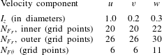
To generate a spatially developing turbulent pipe flow, a turbulent inflow generation technique was required. In the current work, the same procedure was followed as outlined in Sandberg (Reference Sandberg2012), which in summary requires the following steps: at the pipe inlet the mean streamwise velocity, density and temperature profiles obtained from precursor periodic pipe calculations were prescribed. Turbulent fluctuations calculated using a digital filter technique (Touber & Sandham Reference Touber and Sandham2009), using parameters also obtained from the periodic pipe simulations, were superposed onto the mean flow values. The approach by Touber & Sandham (Reference Touber and Sandham2009) of separating the turbulent inlet condition into an inner and outer region was also adopted in the current study and preliminary simulations of turbulent pipe flows confirmed the finding of Touber & Sandham (Reference Touber and Sandham2009) that the digital filter technique is robust to the choice of filter coefficients. All coefficients used for the digital filter in the final jet simulations are compiled in table 1. It was found that the contamination of the previous series of DNS with high levels of internal noise, in particular for the axisymmetric mode (Sandberg & Tester Reference Sandberg and Tester2012; Tester & Sandberg Reference Tester and Sandberg2013), could be partly attributed to the inflow boundary condition outlined above producing mass-flow-rate fluctuations. Therefore, the perturbation velocities of the axisymmetric mode
 $m=0$
were explicitly set to zero at the pipe inlet for the new set of DNS, thus eliminating mass-flow-rate fluctuations in the pipe. Removing velocity fluctuations in
 $m=0$
was found to have no effect on the developed pipe flow downstream.
Coefficients for digital filter technique (Touber & Sandham Reference Touber and Sandham2009). The boundary between inner and outer layers is set to
 $(r-0.5)=0.05$
.

Liner coefficients for all jet Mach numbers
 $M_{jet}$
.
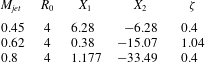
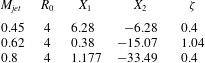
However, removing fluctuations in the axisymmetric mode could not avoid internal noise sources in the higher azimuthal modes contributing to the overall noise field, in particular for Strouhal numbers above their cut-on frequencies. Thus, as an additional measure, a time-domain impedance boundary condition based on a mass–spring–damper analogy, was used, as defined by Tam & Auriault (Reference Tam and Auriault1996). It can be written in a form where the generic resistance parameter
 $R_{0}$
is identified as the dissipative term of the mass–spring–damper model and the two reactance parameters are identified as mass reactance
 $X_{1}$
and stiffness
 $X_{2}$
, which are chosen to produce resonance at the required Strouhal number. For the different jet Mach numbers, the liner parameters were set as listed in table 2. Scalo, Bodart & Lele (Reference Scalo, Bodart and Lele2015) note that a damping ratio
 ${\it\zeta}$
(defined in equation (25b) of Scalo et al.
Reference Scalo, Bodart and Lele2015) greater than unity results in ‘inadmissible (or anti-causal) impedance’. The damping ratio for the coefficient values used is less than unity for the lowest and highest jet Mach numbers but marginally above unity for the jet Mach number 0.62. This did not lead to stability or convergence issues of the DNS solution; however, it should be noted that coefficients originally chosen for the jet Mach number 0.62 case to achieve stronger attenuation were such that the damping ratio was significantly larger than unity and these DNS did experience stability issues. The acoustic liner boundary condition was thoroughly tested in Olivetti et al. (Reference Olivetti, Sandberg and Tester2015) using a pipe configuration terminated with a non-reflecting boundary condition. It was shown that the time-domain model implemented in the DNS solver, using the coefficients listed in table 2, was effective at removing acoustic fluctuations within the pipe without affecting the turbulent flow field, i.e. a fully turbulent pipe flow profile was obtained at the pipe exit.
3.2 Simulation geometry and grid
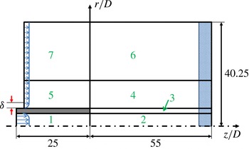
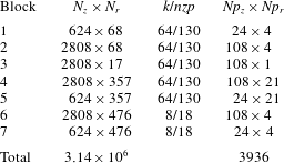
The computational domain is composed of seven blocks, as shown in figure 1: flow inside the pipe (block 1), jet development downstream of the pipe exit (blocks 2, 3, 4 and 6), and co-flow and acoustic field upstream of the pipe exit (blocks 5 and 7). Figure 1 also shows the dimensions of the computational domain, determined from preliminary turbulent pipe and jet simulations (Sandberg et al.
Reference Sandberg, Suponitsky and Sandham2012). The number of grid points in each block and the number of subdomains in the streamwise (
 $z$
) and radial (
 $r$
) directions are given in table 3.
Sketch of the computational domain; the shaded region at the outflow denotes the region in which the zonal characteristic boundary condition (Sandberg & Sandham Reference Sandberg and Sandham2006) was applied.

Number of grid points, Fourier modes
 $k$
/collocation points
 $nzp$
and the number of computing cores for each block in the computational domain (see figure 1).

In the azimuthal direction, 64 or 8 Fourier modes corresponding to 130 or 18 collocation points were used in the turbulent flow (blocks 1 to 5) and acoustic regions (blocks 6 and 7), respectively, resulting in a total of
 $225\times 10^{6}$
grid points.
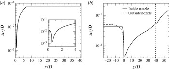
Grid spacing in the radial (a) and axial (b) direction. Vertical dashed line denotes the onset of the zonal characteristic boundary condition (Sandberg & Sandham Reference Sandberg and Sandham2006).

The grid distribution is presented graphically in figure 2. It can be observed that the finest grid spacing was
 ${\rm\Delta}z/D=0.0045$
and
 ${\rm\Delta}r/D=0.00129$
at the nozzle exit. The grid is then stretched up to
 $r/D=6.25$
in the radial direction, from where an equidistant grid with
 ${\rm\Delta}r/D=0.0711$
is maintained up to the free-stream boundary. In the axial direction, the grid is gradually stretched moderately to a maximum grid spacing of
 ${\rm\Delta}z/D=0.05015$
at
 $z/D=39.5$
. The upper bounds of
 ${\rm\Delta}z/D$
and
 ${\rm\Delta}r/D$
were chosen to resolve acoustic waves up to Strouhal number
 $St_{D}\approx 2$
(based on the jet velocity and diameter) with at least 10 grid points.
The turbulent inflow technique described in § 3 is used for the inlet condition of the inside of the pipe. For the inlet boundary of the outside of the pipe, a laminar boundary layer (Blasius solution) was prescribed, reaching
 ${\it\delta}/D=0.025$
at the jet exit. At the outflow boundary a zonal characteristic boundary condition was applied (Sandberg & Sandham Reference Sandberg and Sandham2006), while characteristic boundary conditions were used at the upper free-stream boundary.
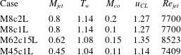
Simulation parameters.

Four different cases were conducted (table 4), all using acoustic liner conditions inside the pipe, to study the Mach-number scaling effect of the jet mixing noise for higher azimuthal modes. The changes in density and temperature were less than 15 % of the wall values, with the wall set to be isothermal at the adiabatic temperature (
 $T_{w}$
given in table 4). All DNS were run for 150 non-dimensional time units (based on diameter and bulk velocity inside the pipe) to allow the initial transients to leave the domain. Each case was then continued for at least 350 time units to achieve statistical convergence. The spatial and temporal resolution of the simulations were rigorously assessed and were found to be adequate (Sandberg et al.
Reference Sandberg, Suponitsky and Sandham2012).
4 Results
4.1 Flow characteristics
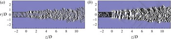
Instantaneous contours of the streamwise density gradient are shown for the near-nozzle region in figure 3 to visualize the turbulent flow exiting the long pipe into the co-flow. The cases M45c1L and M8c2L are compared to each other because both feature roughly the same velocity difference between jet exit and co-flow velocity, i.e. a non-dimensional velocity excess of
 ${\it\lambda}\approx 4$
. For either case, it can be observed that the initial shear layers of the jet are turbulent and do not need to undergo a laminar–turbulent transition, resulting in a rapidly developing turbulent jet. Figure 3 also reveals significant differences between the two cases, such as (the expected) significantly increased amplitudes of the density gradient in the higher-Mach-number case, revealing downstream-radiating sound not seen for the lower jet Mach number at these contour levels, an apparent higher coherence of the shear layer structures in the case with higher jet exit Mach number, and seemingly different spreading rates. The latter observation, however, appears to be associated with the particular time instant at which the two cases are compared, as plotting the time- and azimuthally averaged azimuthal vorticity component (figure 4
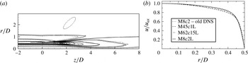
a) reveals that the axial growth of the two jet cases is very similar.
Instantaneous contours of streamwise density gradient near the nozzle: (a) M45c1L case, (b) M8c2L case; with levels [
 $-3\times 10^{-2}$
;
 $3\times 10^{-2}$
].

For a quantitative assessment of the flow exiting the pipe, figure 4(b) shows the time- and azimuthally averaged streamwise velocity profiles of the current DNS and the highest jet Mach number from the previous series of DNS that were conducted without liner boundary condition and unmodified inlet boundary conditions. Case M8c1L is identical to case M8c2L and was omitted for clarity. The profiles were normalized with the centreline value to allow for better comparison of the profiles across Mach numbers. It can be observed that, with increasing Mach number in the pipe, the velocity profiles become fuller. More importantly, overall, it can be observed that the flow exiting the pipe in all cases exhibits a profile reminiscent of a moderate-Reynolds-number fully developed turbulent pipe flow, i.e. the boundary layer thickness of the turbulent flow is relatively thick. This means that the developing jet shear layers will be considerably thicker than those of asymptotically high-Reynolds-number jets, as typically studied in laboratory experiments. The implication of this is that the frequencies associated with the spatial scales of flow events in the pipe interacting with the nozzle lip will be in the same range as those of the jet mixing noise, unlike in high-Reynolds-number jets, where the separation between those two noise generation mechanisms is clear, as will be shown later. However, the objective of the current study is to shed some light on the Mach-number scaling of individual modes of jet mixing noise and the fact that additional noise sources might be in the same frequency range is not seen to be problematic, but rather as an additional challenge for the postprocessing of the DNS data.
(a) Contour lines of time- and azimuthally averaged azimuthal vorticity component for cases M8c2L (solid) and M45c1L (dashed) with 21 levels for range [
 $-$
4; 4]. (b) Time- and azimuthally averaged streamwise velocity profiles, scaled by the centreline velocity, for selected cases from current series of DNS and high jet Mach-number case from previous series of DNS (Sandberg et al.
Reference Sandberg, Suponitsky and Sandham2012), denoted by ‘M8c2 – old DNS’.

Figure 4 also reveals that the flow exiting the pipe for case M8c2L is virtually identical to the case M8c2 from the previous series of DNS, despite the use of a liner boundary condition and the removal of fluctuations in the axisymmetric mode at the pipe inlet boundary in the current case. Sandberg et al. (Reference Sandberg, Suponitsky and Sandham2012) showed for the previous series of DNS that the turbulence statistics at the nozzle exit could be collapsed with profiles in the fully developed region. Owing to the similarity of the current case to the previous DNS result, the flow exiting the pipe can again be considered fully developed and therefore constitutes a well-defined turbulent upstream condition suitable for direct noise computations.
4.2 Acoustic characteristics and source breakdowns
For a qualitative impression of the resulting acoustic field, instantaneous contours of the dilatation field
 $\partial u_{i}/\partial x_{i}$
for an azimuthal slice of the entire axial/radial computational domain are shown in figure 5 for cases M8c2L, M45c1L and the equivalent case from the previous set of DNS (Sandberg et al.
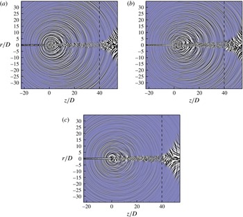
Reference Sandberg, Suponitsky and Sandham2012). For all cases, sound waves can be observed emanating from the end of the pipe (
 $z/D=0$
) and from the jet core. Importantly, no interference of the acoustic field from boundary reflections can be detected, which is particularly encouraging given the very small contour levels chosen (
 $\pm 1\times 10^{-4}$
for the M45c1L case).
For the higher-Mach-number cases, the noise radiation is considerably more directive than for the lower-Mach-number case, with the highest sound radiation intensity observed by visual inspection of the dilatation field at
 ${\it\theta}=30^{\circ }{-}40^{\circ }$
, where
 ${\it\theta}$
is defined with respect to the streamwise direction.
Comparing the new DNS with liner and improved turbulent inflow boundary condition (M8c2L) to the previous M8c2 case reveals striking differences. Firstly, the dilatation field inside the pipe is significantly weaker for the new case, in particular for
 $z/R\geqslant -20$
. Secondly, the acoustic waves emanating from the nozzle and near-jet regions are considerably more directional, indicating a reduction in nozzle-based noise radiation. For all cases, upstream-radiating noise emanating from the nozzle lip can also be detected, although more weakly. Overall, from these figures it would appear that for the lower jet Mach-number case it will be very difficult to extract the jet noise component of the far-field noise in order to investigate the Mach-number scaling.
Instantaneous contours of dilatation field for azimuthal plane
 ${\it\Theta}=0^{\circ },180^{\circ }$
: (a) previous M8c2 case (Sandberg et al.
Reference Sandberg, Suponitsky and Sandham2012), (b) current M8c2L case, both with levels
 $[-5\times 10^{-4};~5\times 10^{-4}]$
; (c) current M45c1L case with levels
 $[-1\times 10^{-4};1\times 10^{-4}]$
.

For that reason, the far-field noise generated by the turbulent jet was investigated with a phased-array technique in order to quantitatively separate the jet mixing noise from any other sources of noise that might be present, e.g. nozzle lip noise. Although such techniques have been available for many years, successful application to large-eddy simulations and DNS data has often been prevented by a combination of two factors: the lack of far-field data and the lack of sufficient time history (record length) to obtain adequate accuracy in the required statistical quantities, such as the spectral density and cross-spectral density of the radiated unsteady pressure.
In the current study, a polar array of virtual microphones has been located at 20 jet nozzle diameters from the nozzle, within the uniform co-flow, having ascertained that the field is obeying the inverse square law at this radius, without any significant reflections from the DNS domain boundaries. The DNS record length, in excess of 350 convective time units for all cases, permits the number of averages for the cross-spectral density to be of order 100 with a filter separation, expressed as a Strouhal number based on the nozzle diameter, of 0.1. A microphone spacing of
 $0.5^{\circ }$
is used over an aperture of
 $140^{\circ }{-}10^{\circ }$
to the jet axis (i.e.
 $40^{\circ }{-}170^{\circ }$
to the ‘intake’ axis), although even finer spacing is available, if required. To assess the contribution of individual azimuthal modes to the overall noise, the pressure PSDs were Fourier-decomposed in the circumferential direction, after removing the pressure non-dimensionalization used for the DNS, to obtain the pressure in pascals.
To understand the acoustic source characteristics of the jet flow in more detail, these polar data have been analysed for each azimuthal mode with a recently developed phased-array code, named AFINDS and described in more detail in Tester, Gabard & Ricoup (Reference Tester, Gabard and Ricoup2012). As well as the usual imaging capability, it is able to extract a ‘noise source breakdown’ using a model in which the jet mixing noise is represented by one or two axially distributed line sources, although in the current work only one jet noise source is used. In addition, two nozzle-based sources are included in the model, each represented by a simple point source, one being a representation of the radiation due to acoustic sources within the jet pipe, the other due to the lip noise source identified previously (Tester & Sandberg Reference Tester and Sandberg2013).
AFINDS is an example of an ‘inverse method’ but differs from most other implementations by allowing for the directivity of each source in the model. It uses a nonlinear least-squares technique to match the observed cross-spectral matrix (CSM) across the polar array with the sum of the CSMs for each source in the model, but only for certain columns in the matrix. The selection corresponds to the choice of ‘reference’ microphones in the array, at which the source image is required for inspection. Conventional beamforming uses all the columns in the matrix but the current approach is preferred for reasons discussed previously (Tester & Glegg Reference Tester and Glegg2010). The key assumptions in AFINDS are: (1) all the sources are mutually incoherent; (2) the initial values of the source positions must be reasonably accurate; (3) each source directivity can be adequately represented by a fourth-order polynomial in the cosine of the polar angle; and (4) the axially distributed jet model can be represented by an analytic function of the form
 $z^{n-1}\exp [-nz/z_{c}]$
(see e.g. Fisher, Harper-Bourne & Glegg Reference Fisher, Harper-Bourne and Glegg1977), where
 $z_{c}$
is the centroid of the axial distribution and
 $n$
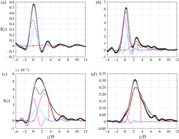
is a symmetry parameter typically in the range 2–4, here taken as 4. The output of the nonlinear least-squares process is a set of estimates for the ‘unknowns’, which are the source intensities, the source directivities and the source positions. The quality of the source breakdown can be inspected by comparing the total DNS image with the AFINDS ‘fitted’ image at the different reference microphones along with the component source images. An example is shown in figure 6(a–d), as viewed at
 $90^{\circ }$
to the jet, for the two lower-Mach-number conditions and azimuthal modes
 $m=0$
and 3. These demonstrate the range of ‘source balance’ in the current study, ranging from a condition where the jet mixing noise source is very weak compared to the two nozzle-based sources to a condition where it dominates. At the lowest flow condition, M45c1L, in figure 6(a),
 $4m=0$
, the two nozzle-based sources dominate and the extremely weak jet noise source is not evident from the DNS source image alone. At the somewhat higher flow Mach number M62c15L, the jet noise is just visible. At the two highest flow conditions for
 $m=0$
, the jet mixing noise dominates, not shown here, but there is still a significant contribution from the nozzle-based sources. At the lowest flow condition for
 $m=3$
in figure 6(c), all three sources are comparable, but without this source breakdown process, the DNS image could be misinterpreted as a single jet mixing noise source. Similarly for the higher-Mach-number condition in figure 6(d), the two nozzle-based sources cause a weak ripple in the DNS source image, not unlike ripples elsewhere in the image. This figure also shows how well the analytic jet noise model fits the data.
Source images for
 $St_{D}=1$
at
 $90^{\circ }$
to the jet: (a) M45c1L,
 $m=0$
, (b) M62c15L,
 $m=0$
, (c) M45c1L,
 $m=3$
, (d) M62c15L,
 $m=3$
. The open black symbols represent the image of the DNS data, and the solid lines show the AFINDS fits. The solid red line represents the AFINDS source breakdown image of the jet noise source, the solid magenta line the first nozzle-based source (internal noise) and the solid cyan line the second nozzle based source (lip noise).

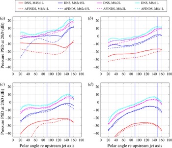
Using the AFINDS source intensity and directivity coefficients, the jet mixing noise source level and directivity may be compared with those of the DNS, which contains all the sources, over the whole polar arc. Figure 7 shows this comparison for all four flow conditions for each azimuthal mode. As indicated from the source image examples in figure 6, the DNS radiation is largely dominated by the nozzle-based sources at M45c1L, except for
 $m=3$
. At the highest Mach number, for both co-flow values, M8c2L and M8c1L, the jet noise dominates except in the forward arc (polar angle
 ${<}90^{\circ }$
). It is also of interest to note that the directivity of the AFINDS jet mixing noise for the axisymmetric mode
 $m=0$
in figure 7(a) exhibits a sharp increase at small angles to the jet axis for the two lower jet Mach numbers M45c1L and M62c15L, very much like the ‘superdirectivity’ identified previously by Cavalieri et al. (Reference Cavalieri, Jordan, Colonius and Gervais2012). Their experiments covered the acoustic Mach-number range 0.4–0.6, which is similar to that encompassed by our two lower flow conditions. At our two higher flow conditions the superdirectivity is less obvious, with both the DNS and AFINDS jet noise following a smooth pattern more like those of the higher-order azimuthal modes. Overall, for the axisymmetric mode, which dominates the overall noise field, the peak directivity is seen to be at around
 $30^{\circ }$
or less to the jet axis.
Comparison of DNS total directivity and AFINDS jet noise directivity (PSD, dB) at
 $St_{D}=1$
for the four jet flow conditions (see table 4): (a)
 $m=0$
, (b)
 $m=1$
, (c)
 $m=2$
, (d)
 $m=3$
.

To help understand these results, it is worth mentioning that AFINDS has also been used to compare case M8c2L to another DNS case using the same flow parameters and overall set-up, but without the liner boundary condition, which quantified the effect of the acoustic liner model on the respective contributions from the nozzle based and the jet mixing noise sources. The results obtained from the noise source breakdown showed that the liner only marginally affects the axisymmetric mode while being very effective at reducing nozzle-based noise contributions in the higher azimuthal modes (Sandberg & Tester Reference Sandberg and Tester2014). The scaling properties of these jet mixing noise levels are studied in the following section.
4.3 Mach-number scaling
Based upon the AFINDS source breakdown technique, the Mach-number scaling of the jet noise component for all jet Mach numbers is considered in our new series of DNS. In this study we consider scaling of the radiated sound field mainly at
 $90^{\circ }$
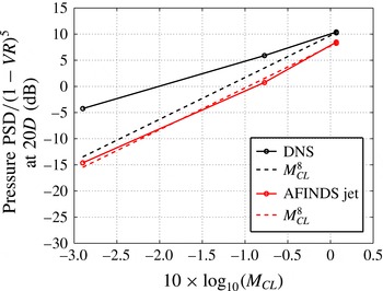
to the jet axis, which is closely related to the jet mixing noise source strength and essentially free of any convection or refraction effects. The resulting Mach-number scaling is shown in figure 8 for a normalized PSD summed over the axisymmetric mode
 $m=0$
and the higher azimuthal modes
 $m=1$
,
 $2$
and
 $3$
for a Strouhal number of
 $St_{D}=1$
. This frequency was chosen because the acoustic liner boundary condition used inside the pipe was set to resonate at this frequency and it was therefore expected that the jet noise component would be least contaminated by internal noise at this frequency. Note that the PSD is plotted versus the Mach number based on the centreline velocity.
Mach-number scaling of the jet noise component at
 $90^{\circ }$
for
 $St_{D}=1.0$
. The open black symbols with solid line represent the DNS data, dashed lines show
 $M^{8}$
scaling (based on jet axis velocity), and red open symbols with solid line are the AFINDS fit for the jet noise component of the overall noise field.

In figure 8, the PSD at
 $90^{\circ }$
and distance 20 diameters from the nozzle for
 $St_{D}=1.0$
is normalized by
 $(1-u_{co}/u_{CL})^{5}$
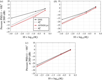
to account for jet noise co-flow effects, based on previous experimental studies. Note that four data points are included, one each for the cases M45c1L, M62c15L, M8c1L and M8c2L, with the latter two being at the same location of the horizontal axis. The scaling obtained from DNS directly corresponds approximately to an
 $M^{5}$
scaling, indicating that, in addition to jet mixing noise, there are other noise sources present, such as, for example, nozzle lip noise. However, when performing the source breakdown using AFINDS to separate out the jet noise source, the expected Mach-number scaling of
 $M^{8}$
is obtained, particularly accurately for
 $M_{jet}>0.62$
, a well-established scaling law for isothermal jet noise, both experimentally (Viswanathan Reference Viswanathan2006) and theoretically. This result is very encouraging in two respects. Firstly, it demonstrates the capability of AFINDS to extract the jet noise source from the overall acoustic field, and secondly it shows that the series of DNS solutions is capturing the expected physics over a wide range of jet Mach numbers and realistic co-flows.
Mach-number scaling of the jet noise component at
 $90^{\circ }$
for
 $St_{D}=1.0$
for azimuthal Fourier modes (a)
 $m=0$
, (b)
 $m=1$
and (c)
 $m=3$
. Symbols and lines as described in the caption of figure 8.

In order to produce the following figures, the far-field pressure field was decomposed into azimuthal Fourier modes in order to investigate the Mach-number scaling of the individual circumferential modes. In figure 9 the total pressure PSD at
 $St_{D}=1.0$
, displayed the same way as in figure 8 and from the same spatial location, is shown for modes
 $m=0$
,
 $m=1$
and
 $m=3$
. The picture for
 $m=0$
is very similar to that of the total noise field, i.e. the scaling of the raw data is nowhere close to
 $M^{8}$
scaling, while the jet noise source extracted from the data using the noise source breakdown technique agrees very well with the theoretical prediction. However, when considering
 $m=0$
only, a near-exact
 $M^{8}$
scaling is obtained across all simulated Mach numbers, implying that when considering all Fourier modes there are some contributions from higher modes at the lowest jet Mach number that cause the scaling to slightly deviate from an eighth power law (cf. figure 8). This is in contrast to the velocity exponent of just over 7 found for jets in static conditions by Cavalieri et al. (Reference Cavalieri, Jordan, Colonius and Gervais2012) for
 $m=0$
at
 $St_{D}=0.2$
. When investigating the behaviour of
 $m=1$
, several observations can be made. First, the raw DNS data now display an
 $M^{8}$
scaling when considering only cases M62c15L, M8c1L and M8c2L. This implies that the liner boundary conditions used in the DNS are removing most of the internal noise sources and therefore the overall far-field noise mainly comprises jet mixing noise in these cases. At the lowest jet Mach number simulated, extracting the jet noise source using AFINDS is required in order to obtain a Mach-number scaling with approximately eighth power. For
 $m=3$
, the behaviour described for
 $m=1$
is even clearer, with the DNS raw data coming even closer to an eighth power-law scaling (implying even better performance by the liner boundary conditions) and the AFINDS jet noise source exhibiting a nearly perfect
 $M^{8}$
scaling across all jet Mach numbers investigated.
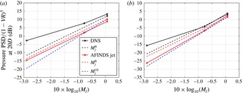
Mach-number scaling of the jet noise component at
 $90^{\circ }$
for
 $St_{D}=0.4$
for azimuthal Fourier modes (a)
 $m=0$
and (b)
 $m=1$
. Symbols and lines as described in the caption of figure 8, but with additional
 $M^{10}$
scaling line.

The crucial and, to the authors’ knowledge, formerly unknown finding is that for
 $St_{D}=1.0$
it appears as if all azimuthal Fourier modes adhere to the same Mach-number scaling for co-flowing jets at
 $90^{\circ }$
to the jet axis.
In order to assess whether the Mach-number scaling of the individual azimuthal modes is not confined to
 $St_{D}=1$
, two additional Strouhal numbers were investigated, one significantly lower,
 $St_{D}=0.4$
, corresponding to the peak in the power spectral density, and one significantly higher,
 $St_{D}=1.4$
. The results are shown in figures 10 and 11. The results for the lower frequency are similar to those at
 $St_{D}=1$
. For the axisymmetric mode, again we extract the jet noise source using AFINDS and find a Mach-number scaling with an exponent very close to eight. For higher modes (mode
 $m=1$
is shown), using the raw DNS data,
 $M^{8}$
scaling can only be observed for the higher jet Mach-number cases. Looking at the jet noise source only, extracted with AFINDS, we find the scaling for
 $m=1$
is actually closer to an
 $M^{10}$
scaling.
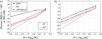
Mach-number scaling of the jet noise component at
 $90^{\circ }$
for
 $St_{D}=1.4$
for azimuthal Fourier modes (a)
 $m=0$
and (b)
 $m=1$
. Symbols and lines as described in the caption of figure 8, but with additional
 $M^{10}$
scaling line.

At the higher frequency
 $St_{D}=1.4$
(figure 11), the picture is less clear than for the lower Strouhal numbers considered. For the axisymmetric mode, the raw DNS data do not give a constant Mach-number scaling over the range of jet Mach numbers simulated and for no segment is close to an eighth power law. When isolating the jet noise source with AFINDS, the Mach-number scaling between cases with
 $M_{jet}=0.45$
and
 $M_{jet}=0.8$
is weaker than
 $M^{8}$
. However, the case M62c15L does not fall on the same line and requires further investigation. For the first azimuthal mode
 $m=1$
, the acoustic liner boundary condition again appears to serve its purpose well and the data obtained from the raw data and from AFINDS produce nearly the same line, except for an amplitude increase of approximately 4 dB for the DNS data. Despite being very similar, both exhibit a scaling with an exponent slightly lower than eight and similar to that of the axisymmetric mode, if case M62c15L is excluded. For the moment a clear reason for why the Mach-number scaling of the jet noise source changes for higher frequencies cannot be given. However, one possible explanation is that the DNS jet noise spectra appear to roll off more rapidly than typical measured narrow-band spectra of high-Reynolds-number jets and the resulting lower amplitudes at higher frequencies might be a challenge for the postprocessing.
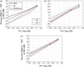
Mach-number scaling of the jet noise component for
 $St_{D}=1$
for azimuthal Fourier mode
 $m=0$
at (a)
 $60^{\circ }$
and (b)
 $30^{\circ }$
to the jet axis and (c) for mode
 $m=1$
at
 $30^{\circ }$
. Symbols and lines as described in the caption of figure 8, with the addition of a tenth power line through the M8c1L point.

Finally in figure 12 results are presented for angles other than
 $90^{\circ }$
, specifically for
 $60^{\circ }$
and
 $30^{\circ }$
to the jet axis, and the first two modes
 $m=0$
and 1. At
 $60^{\circ }$
the AFINDS result for the axisymmetric mode does not show a clear scaling over the entire Mach-number range. However, if neglecting the M62c15L case, the scaling appears to be much closer to an exponent of 10 than 8. At the smaller angle of
 $30^{\circ }$
the results obtained with AFINDS more clearly suggest an
 $M^{10}$
scaling. It should be noted that the tenth power line is anchored to the M8c1L point for all cases, as the co-flow effect is not scaled accurately at these small angles, as exemplified by the large offset of the M8c2L point at the smallest angle considered (figure 12
b). For the first azimuthal mode
 $m=1$
, at
 $30^{\circ }$
the AFINDS result is again close to an
 $M^{10}$
scaling. This agrees with exponents from measured data for angles close to the jet axis (Viswanathan Reference Viswanathan2006) which approach 10 for the isothermal jet.
In order to be able to generalize the above results to high-Reynolds-number turbulent jets with considerably thinner nozzle boundary layers, a thorough study in which the inlet boundary layer thickness, fluctuation level, azimuthal organization and jet Reynolds number are all varied would be desirable. The phased-array and source breakdown analysis of data for the individual azimuthal modes presented in the current paper could again be applied; however, the far-field pressure data could be provided by carefully executed laboratory experiments to avoid unnecessarily high computational cost.
5 Conclusions
A series of DNS of fully turbulent flow exiting a long pipe were conducted at target Reynolds number, based on jet exit velocity at the axis, of
 $Re_{jet}=8000$
, for varying jet exit and co-flow Mach numbers.
The main objective of the work was to investigate the Mach-number scaling of the jet noise for individual azimuthal Fourier modes. In order to assess pure jet mixing noise, a number of challenges had to be overcome. Firstly, based on previous experience with DNS of pipe–jet configurations, several key features were required to be included in the simulations to produce as clean a jet noise field as possible. To suppress possible internal noise sources emanating from the pipe exit and contaminating the acoustic far field, an acoustic liner model was applied to the interior nozzle walls. In addition, the turbulent inflow generation technique was modified to be free of velocity fluctuations in the axisymmetric mode. Furthermore, despite the DNS producing a much cleaner jet noise field than earlier simulations, the use of a source breakdown code was essential in order to isolate the jet noise source from the overall noise field, in particular for the axisymmetric mode
 $m=0$
.
Despite the significant reduction of unwanted noise source within the pipe, the use of a phased-array source breakdown technique was essential to isolate the jet noise source, in particular for the axisymmetric mode. For the Reynolds and Mach numbers simulated with DNS, it is found that the overall jet noise sources, i.e. the sum of the azimuthal modes, shows the expected
 $M^{8}$
scaling with the centreline jet Mach number when accounting for co-flow effects by scaling the results with
 $(1-u_{co}/u_{CL})^{5}$
. More importantly, the DNS results also suggest that the individual azimuthal modes exhibit the same scaling, at least for Strouhal numbers up to
 $St_{D}=1$
. At higher frequencies, a consistent scaling over the entire
 $M_{jet}$
range could not be found and the exponent is lower than eight. The reason for this behaviour is still unknown and is the subject of a current investigation. The main emphasis has been on
 $90^{\circ }$
, as the
 $M^{8}$
scaling with the jet exhaust Mach number and co-flow Mach number is well established. However, initial results at two other angles,
 $60^{\circ }$
and
 $30^{\circ }$
, were also generated with the phased-array source breakdown technique and indicate an increase of the velocity exponent of the jet noise source towards 10 at
 $30^{\circ }$
, with the higher azimuthal modes again showing the same behaviour as the axisymmetric mode.
Acknowledgements
Fruitful discussions with Professor C. L. Morfey are gratefully acknowledged. Computer time was provided by the UK Turbulence Consortium under EPSRC grant EP/L000261/1.