1 Introduction
Low-density jets have attracted considerable attention over the last few decades as a result of their role in industrial processes such as fuel injection and plasma spraying. Under certain conditions, such jets can develop global hydrodynamic instability, leading to self-excited oscillations at a limit cycle (Sreenivasan, Raghu & Kyle Reference Sreenivasan, Raghu and Kyle1989; Huerre & Monkewitz Reference Huerre and Monkewitz1990; Monkewitz et al. Reference Monkewitz, Bechert, Barsikow and Lehmann1990). On the one hand, such oscillations can be beneficial in situations where mixing is desired. On the other hand, they can be detrimental in situations where they excite unwanted acoustic or structural resonances. Therefore, it is important to be able to predict the onset of global hydrodynamic instability as well as the frequency and amplitude of the resulting limit-cycle oscillations (LCOs).
1.1 Bifurcation of a low-density jet
Raghu & Monkewitz (Reference Raghu and Monkewitz1991) have shown that a low-density jet becomes globally unstable via a Hopf bifurcation: after a critical point (the Hopf point), the jet becomes unstable to infinitesimal perturbations and transitions to a self-excited state characterised by LCOs. Near the Hopf point, the growth rate is small, implying that the oscillation amplitude (
 $a$
) evolves much more slowly than the oscillation frequency (
 $\unicode[STIX]{x1D714}$
) (Raghu & Monkewitz Reference Raghu and Monkewitz1991). Landau (Reference Landau1944) proposed an equation to model the amplitude evolution in this specific regime, which Stuart (Reference Stuart1960) later formulated for plane Poiseuille flow using an energy balance. This has become known as the Stuart–Landau equation:
 $$\begin{eqnarray}\frac{\text{d}a}{\text{d}t}=k_{1}a+k_{2}a^{3}+\cdots \,,\end{eqnarray}$$
where
 $t$
is time,
 $k_{1}$
is a linear driving/damping parameter and
 $k_{2}$
is a nonlinear parameter. The Hopf point is at
 $k_{1}=0$
, after which (
 $k_{1}>0$
) the system becomes linearly unstable.
The Hopf bifurcation in low-density jets is usually considered to be supercritical (Monkewitz et al.
Reference Monkewitz, Bechert, Barsikow and Lehmann1990; Raghu & Monkewitz Reference Raghu and Monkewitz1991), i.e. LCOs cannot occur before the Hopf point (
 $k_{1}<0$
). Therefore, the linear parameter (
 $k_{1}$
) alone determines the stability boundaries of the system. However, Sreenivasan et al. (Reference Sreenivasan, Raghu and Kyle1989) observed a hysteretic regime in which LCOs can occur even when
 $k_{1}<0$
. This led Kyle & Sreenivasan (Reference Kyle and Sreenivasan1993) to suggest that the Hopf bifurcation in low-density jets can also be subcritical, which Zhu, Gupta & Li (Reference Zhu, Gupta and Li2017) later formally established. In a system with a subcritical Hopf bifurcation, a finite-amplitude perturbation can trigger the system to LCOs via contributions from the nonlinear terms (such as
 $k_{2}a^{3}$
) even when
 $k_{1}<0$
. This regime, where LCOs can occur despite the system being linearly stable, is called the bistable regime.
An important implication from the existence of a subcritical bifurcation in a system is that the nonlinear terms need to be calculated before the stability boundaries can be determined. The challenge, however, is that existing methods applied to jets (Raghu & Monkewitz Reference Raghu and Monkewitz1991) and wakes (Provansal, Mathis & Boyer Reference Provansal, Mathis and Boyer1987; Dusek, Le Gal & Fraune Reference Dusek, Le Gal and Fraune1994; Sipp & Lebedev Reference Sipp and Lebedev2007) can only calculate the nonlinear terms from measurements of the system dynamics after the emergence of LCOs. In other words, such methods can describe the system behaviour via post-processing, which is itself useful, but they lack predictive capabilities, particularly for nonlinearities.
1.2 Bifurcation analysis and system identification of fluid dynamical systems
In most fluid dynamical systems, it is important to know where the bifurcation points are, as they determine the stability boundaries. The most direct way of finding the bifurcation points is to solve the time-dependent Navier–Stokes equations and determine the parameter value (e.g. the Reynolds number,
 $Re$
) at which the flow undergoes a qualitative change in behaviour. Alternatively, one can obtain steady solutions of the system at a lower computational cost, and then solve for the eigenvalues of its Jacobian matrix (Jackson Reference Jackson1987; Dijkstra et al.
Reference Dijkstra, Wubs, Cliffe, Doedel, Dragomirescu, Eckhardt, Gelfgat, Hazel, Lucarini, Salinger, Phipps, Sanchez-Umbria, Schuttelaars, Tuckerman and Thiele2014). However, if applied to systems with complex geometries or boundaries, such direct methods can be expensive and unreliable, as it is often difficult to define the boundary conditions with sufficient accuracy to produce meaningful numerical solutions (Kim & Moin Reference Kim and Moin1985; Thompson & Troian Reference Thompson and Troian1997). In such cases, one needs to first identify the system using the data available and then determine its bifurcation points. System identification (SI) methods for this purpose can be divided into two classes: (i) purely data-driven methods and (ii) hybrid methods.
In purely data-driven methods, the governing equations of a physical system are found exclusively from experimental data, without the need to assume a system model a priori. For example, Schmidt & Lipson (Reference Schmidt and Lipson2009) used symbolic regression to identify the nonlinear differential equations governing a variety of physical systems, ranging from simple harmonic oscillators to chaotic double pendula. In that procedure, experimental data are fitted to simple mathematical building blocks based on Hamiltonians and Lagrangians. New equations are then added to these via genetic programming. Although useful for simple systems, symbolic regression becomes impractical for systems containing a large number of degrees of freedom. To overcome this problem, Brunton, Proctor & Kutz (Reference Brunton, Proctor and Kutz2016) recognised that the key dynamics of most physical systems is usually simple enough to be described by just a few leading terms. This makes it possible to use sparsity-promoting tools and machine learning to identify low-dimensional models of physical systems at a reduced computational cost. Recently, Shimizu & Kawahara (Reference Shimizu and Kawahara2018) also used machine learning to determine the low-dimensional equations governing low-
 $Re$
turbulence in plane Couette flow, enabling the entire bifurcation cascade to be reproduced and studied.
Purely data-driven methods for SI are useful for their role in explaining many naturally occurring phenomena for which there is an abundance of experimental data but nearly no knowledge of the governing equations. In engineering situations, however, collecting experimental data is usually expensive, but there is often some knowledge of the underlying system dynamics. Therefore, for such situations, a hybrid method may be more suitable. In hybrid methods, an appropriate low-dimensional model is assumed for the system, and then experimental data are used to determine the parameter values of the model and their variations with the physical parameters of the system (Price & Valerio Reference Price and Valerio1990; Thothadri & Moon Reference Thothadri and Moon2005). For example, (1.1) can be assumed to be a low-dimensional model of a jet or wake in the vicinity of a Hopf bifurcation. Variations in
 $k_{1}$
and
 $k_{2}$
with
 $Re$
can then be extracted from experimental data, as demonstrated by Provansal et al. (Reference Provansal, Mathis and Boyer1987) and Raghu & Monkewitz (Reference Raghu and Monkewitz1991). These conventional methods, however, are limited to nearly noise-free measurements and to systems with a supercritical Hopf bifurcation.
Recently, Noiray & Schuermans (Reference Noiray and Schuermans2013) and Boujo & Noiray (Reference Boujo and Noiray2017) have extended the aforementioned SI methods to exploit the influence of noise, which, in their experiments, came from background turbulence in the flow field of a thermoacoustic system. They replaced the Stuart–Landau equation with its corresponding Fokker–Planck equation, yielding expressions for the probability density function, which is equivalent to the long-time average of the noise-affected measurements. Bonciolini et al. (Reference Bonciolini, Ebi, Boujo and Noiray2018) further extended this method to enable SI of a laboratory-scale combustor undergoing a subcritical Hopf bifurcation. However, to be able to determine the nonlinear terms, all of these SI methods require at least some data from the LCO regime. Consequently, these methods cannot predict the nature of a bifurcation or the resulting LCO dynamics. In fact, in most of these methods, the nonlinear terms are ignored in the regime before the Hopf point (
 $k_{1}<0$
) (Provansal et al.
Reference Provansal, Mathis and Boyer1987). By contrast, Zhu (Reference Zhu2017, chap. 3) has shown from the noise-induced dynamics of a low-density jet that the nonlinear terms are active even before the stability boundaries are reached, i.e. in the unconditionally stable regime, where the system is stable to infinitesimal as well as finite-amplitude perturbations.
1.3 Noise-induced dynamics: coherence resonance
In a pioneering work, Wiesenfeld (Reference Wiesenfeld1985) explored the effect of noise on oscillatory systems and found that the spectra of the noise-induced dynamics contain precursors capable of forecasting impending nonlinear instabilities. In particular, it was found that the system response to noise becomes more coherent (or less noisy) on approach to the Hopf point. Later, Pikovsky & Kurths (Reference Pikovsky and Kurths1997) found for the FitzHugh–Nagumo system that the coherence in the noise-induced dynamics first increases, reaches a maximum and then decreases as the noise amplitude increases. They termed this phenomenon coherence resonance. Ushakov et al. (Reference Ushakov, Wünsche, Henneberger, Khovanov, Schimansky-Geier and Zaks2005) formally defined coherence resonance in terms of the coherence factor and showed that systems with Hopf bifurcations generally exhibit some degree of coherence resonance.
Recently, Kabiraj et al. (Reference Kabiraj, Steinert, Saurabh and Paschereit2015) and Zhu (Reference Zhu2017) reported coherence resonance in two different fluid dynamical systems: a thermoacoustic oscillator and a low-density jet, respectively. Gupta et al. (Reference Gupta, Saurabh, Paschereit and Kabiraj2017) phenomenologically modelled coherence resonance in a thermoacoustic system, enabling the noise-induced dynamics arising from supercritical and subcritical Hopf bifurcations to be explored in detail. Moreover, Zhu (Reference Zhu2017) experimentally demonstrated the use of coherence resonance to identify the different types of Hopf bifurcation in a low-density jet via the noise-induced dynamics in only the unconditionally stable regime. However, information obtained in this specific regime has yet to be exploited for SI of any experimental system – fluid dynamical or otherwise.
1.4 Contributions of the present study
In this paper, we develop an SI framework that uses data from only the unconditionally stable regime to predict the nonlinear behaviour of a low-density jet in the vicinity of its Hopf bifurcation. Specifically, we aim to predict (i) the order of nonlinearity, (ii) the locations and types of the bifurcation points (and hence the stability boundaries) and (iii) the resulting LCO dynamics – without having to operate the system in the potentially dangerous linearly unstable or bistable regimes.
Below, we present the experimental data and SI methodology in §§ 2 and 3, respectively. We then show the results in § 4 in terms of the order of nonlinearity, dynamic and stochastic bifurcations and the LCO dynamics beyond the bifurcation points, before concluding in § 5.
2 Experimental data
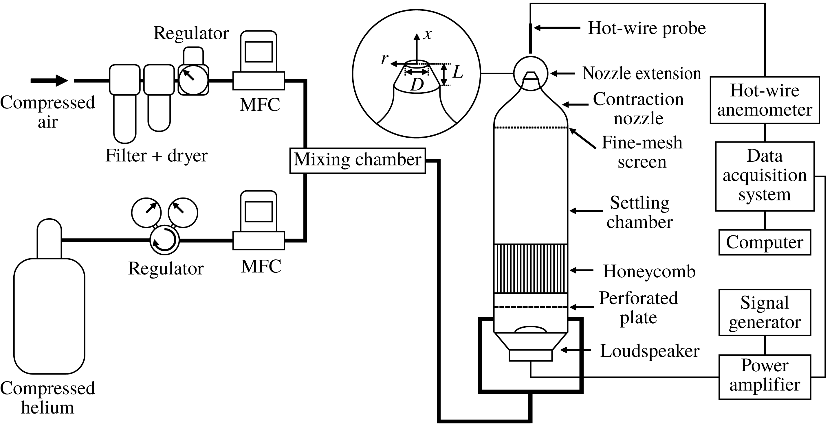
We use the experimental data from Zhu (Reference Zhu2017). Figure 1 shows the set-up used to collect the data, which consists of an axisymmetric nozzle assembly, an acoustic forcing system, gas supply lines and a hot-wire anemometer. In this set-up, a laminar helium–air jet discharging into quiescent ambient air is perturbed by external noise. There are three main independent control parameters governing the stability boundaries of the jet and its LCO dynamics. These are (i) the jet-to-ambient density ratio,
 $S\equiv \unicode[STIX]{x1D70C}_{j}/\unicode[STIX]{x1D70C}_{\infty }$
, (ii) the aspect ratio of the nozzle tip,
 $L/D$
, which controls the thickness of the initial shear layer, and (iii) the jet Reynolds number,
 $Re\equiv \unicode[STIX]{x1D70C}_{j}U_{j}D/\unicode[STIX]{x1D707}_{j}$
, where
 $U_{j}$
is the jet centreline velocity,
 $D$
is the nozzle exit diameter and
 $\unicode[STIX]{x1D707}_{j}$
is the dynamic viscosity of the jet fluid. In this paper, we keep the first two parameters fixed and vary only
 $Re$
.
A schematic of the experimental set-up used to produce a low-density jet perturbed by external noise (Zhu Reference Zhu2017). MFC: mass flow controller.
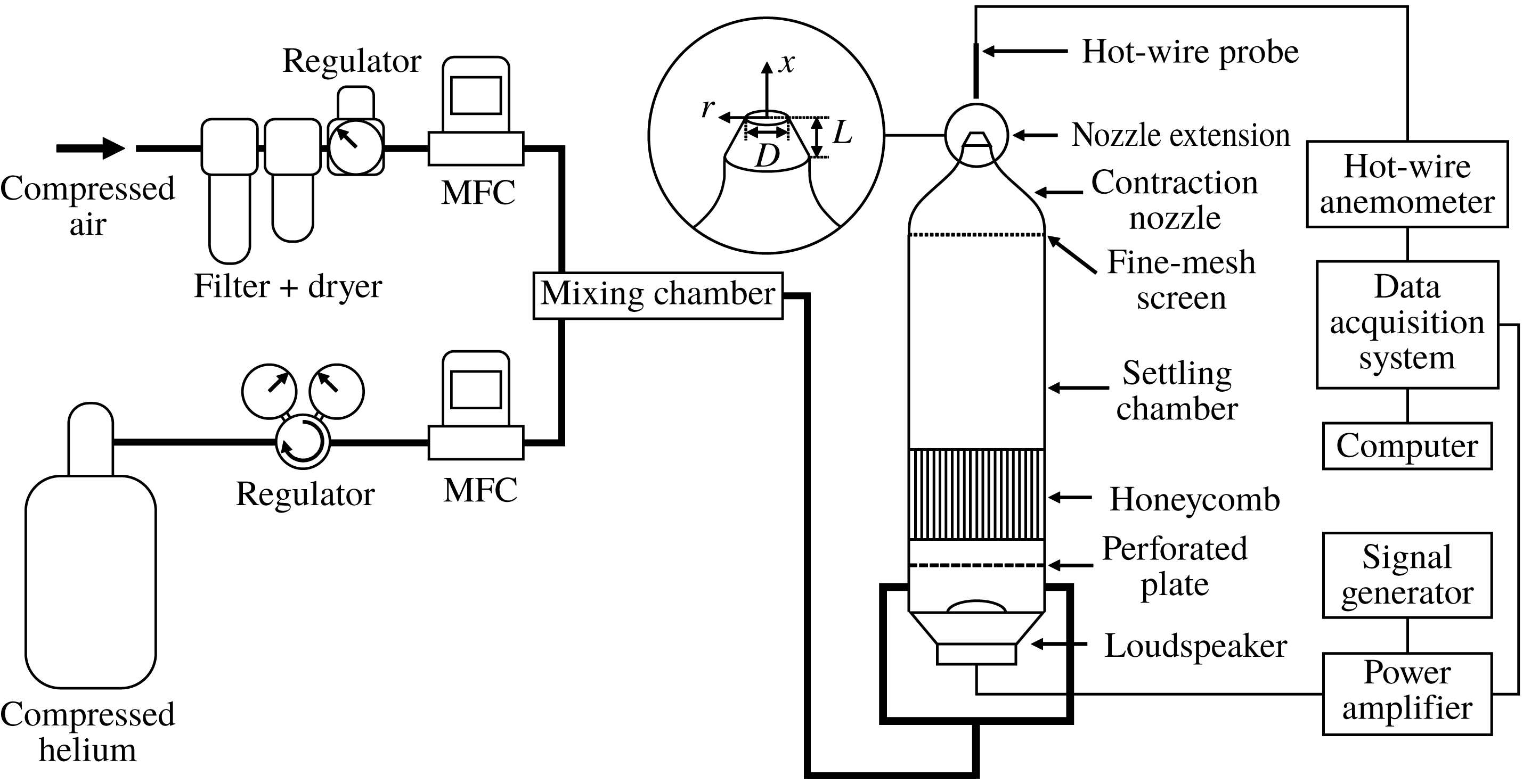
The acoustic forcing system consists of three components: (i) a signal generator (Keysight 33512B), (ii) a power amplifier (Alesis RA150), and (iii) a loudspeaker (FaitalPRO 3FE25). The signal generator produces Gaussian noise with a bandwidth of 0–20 MHz. The upper frequency limit of the noise (20 MHz) is four orders of magnitude higher than the natural global frequency of the jet. Therefore, the noise felt by the jet is essentially white. The noise amplitude is controlled by regulating the input voltage into the loudspeaker (
 $V$
) with the power amplifier. The noise-induced dynamics of the jet is measured in terms of the local streamwise velocity in the potential core, using a hot-wire probe positioned on the jet centreline,
 $1.5D$
downstream from the jet exit. The output voltage from the hot-wire probe is digitised at a frequency of 32 768 Hz. Further details on these measurements can be found in Zhu (Reference Zhu2017).
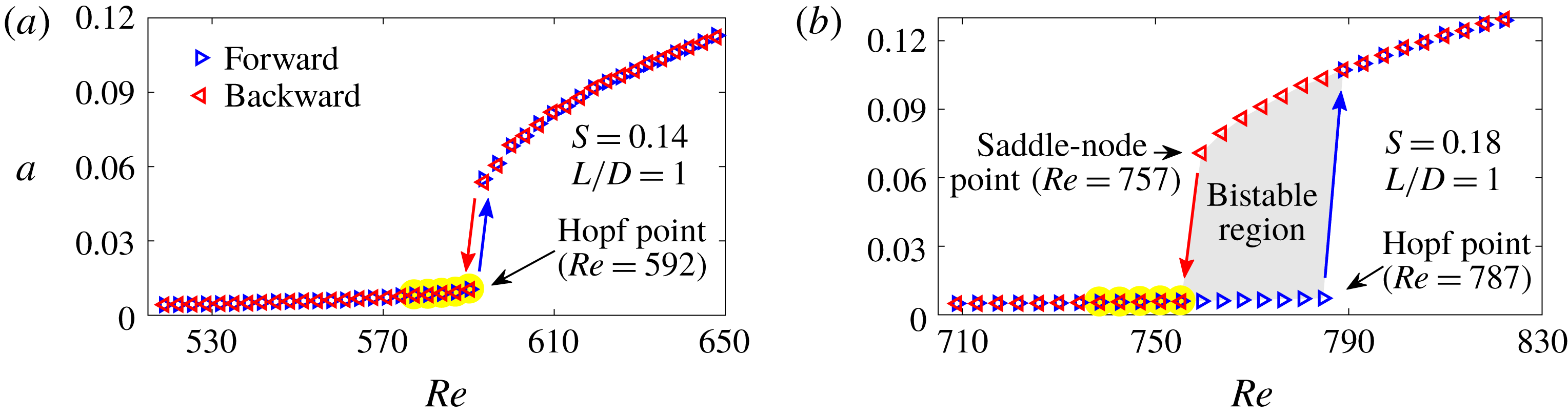
Bifurcation diagrams for two experimental cases: (a) ExpSuper and (b) ExpSub. In the legend, the terms ‘forward’ and ‘backward’ refer to data collected by increasing and decreasing
 $Re$
, respectively. The data used for SI are collected exclusively in the unconditionally stable regime, as highlighted in yellow.
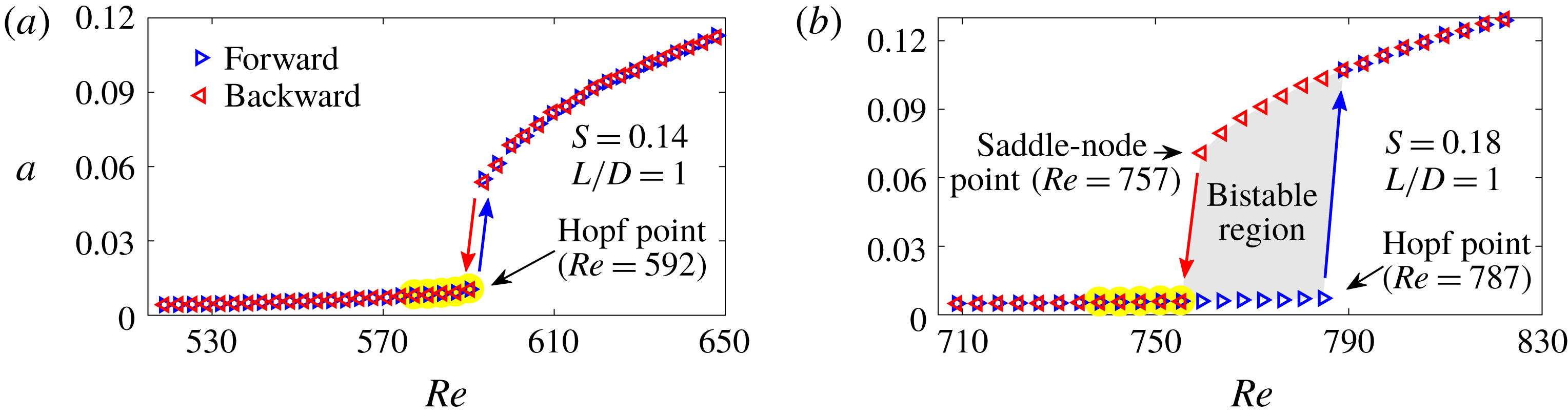
We consider two representative flow conditions, whose bifurcation diagrams are shown in figure 2. In figure 2(a), where
 $S=0.14$
and
 $L/D=1$
, the Hopf point is at
 $Re=592$
, below which LCOs are not observed. Thus, this condition is experimentally determined to be supercritical and is called ExpSuper here. In figure 2(b), where
 $S=0.18$
and
 $L/D=1$
, the Hopf point is at
 $Re=787$
, below which LCOs are observed down to
 $Re=757$
, which is a saddle-node point. Thus, this condition is experimentally determined to be subcritical and is called ExpSub here. In this study, the data used for SI are collected exclusively in the unconditionally stable regime, which is highlighted in yellow in figure 2.
3 Methodology for system identification
3.1 System model
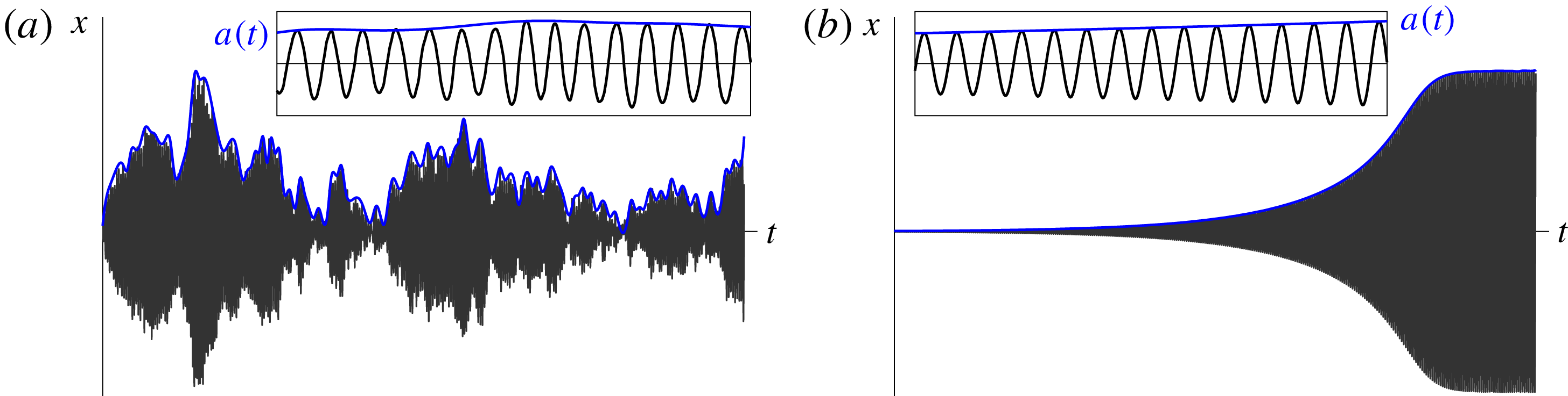
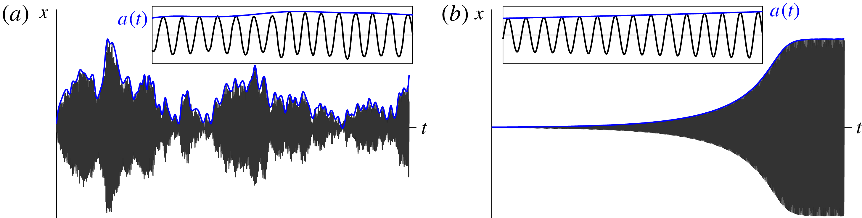
Figure 3 shows cartoon drawings relating the oscillation amplitude,
 $a(t)$
, to the instantaneous state of the system,
 $x(t)$
, e.g. velocity measurements from a hot-wire probe, for (a) a marginally unconditionally stable regime and (b) a marginally linearly unstable regime. For both regimes, the evolution of
 $a(t)$
, which can be approximated by a Stuart–Landau equation, is at a much slower rate than that of
 $x(t)$
. The effect of noise on the system is felt via
 $x(t)$
, for which we assume the following governing equation:
 $$\begin{eqnarray}\ddot{x}-(\unicode[STIX]{x1D716}+\unicode[STIX]{x1D6FC}_{1}x^{2}+\unicode[STIX]{x1D6FC}_{2}x^{4}+\unicode[STIX]{x1D6FC}_{3}x^{6}+\unicode[STIX]{x1D6FC}_{4}x^{8}+\cdots ){\dot{x}}+x+\unicode[STIX]{x1D6FD}x^{3}=\sqrt{2d}\unicode[STIX]{x1D702}(t),\end{eqnarray}$$
where
 $\unicode[STIX]{x1D702}(t)$
is a unit additive white Gaussian noise term representing the effect of the loudspeaker,
 $d$
is its amplitude,
 $\unicode[STIX]{x1D716}$
is the linear growth/damping term,
 $\unicode[STIX]{x1D6FC}_{1},\unicode[STIX]{x1D6FC}_{2},\unicode[STIX]{x1D6FC}_{3}$
,
 $\unicode[STIX]{x1D6FC}_{4},\ldots$
are the nonlinear system parameters and
 $\unicode[STIX]{x1D6FD}$
is the anisochronicity factor, which controls the shift in oscillation frequency with amplitude. Equation (3.1) is non-dimensionalised such that (i) the natural frequency is fixed at 1 for all
 $Re$
and (ii)
 $x\equiv u^{\prime }/\overline{u}$
, where
 $u^{\prime }$
is the measured velocity fluctuation and
 $\overline{u}$
is its time average. Here
 $\unicode[STIX]{x1D6FC}_{1}$
is a counterpart to
 $k_{2}$
in (1.1) and determines the nature of the Hopf bifurcation.
Evolution of
 $a(t)$
and
 $x(t)$
for (a) noise-induced dynamics in the marginally unconditionally stable regime and (b) noise-free limit-cycle development in the marginally linearly unstable regime. In both cases, the evolution of
 $a(t)$
is slower than that of
 $x(t)$
.
To derive the probabilistic solution of (3.1), we first use the method of variation of parameters (Nayfeh & Mook Reference Nayfeh and Mook1979; Nayfeh Reference Nayfeh1981), transforming the instantaneous state of the system (
 $x$
) into its amplitude (
 $a$
) and phase (
 $\unicode[STIX]{x1D719}$
):
 $$\begin{eqnarray}x(t)=a(t)\cos (t+\unicode[STIX]{x1D719}(t)).\end{eqnarray}$$
This leads to two equations (3.1) and (3.2) in three unknowns:
 $x(t)$
,
 $a(t)$
and
 $\unicode[STIX]{x1D719}(t)$
. Thus, we can impose a third condition that is independent of (3.1) and (3.2). Following Nayfeh (Reference Nayfeh1981), we take this condition to be
 $$\begin{eqnarray}{\dot{x}}(t)=-a(t)\sin (t+\unicode[STIX]{x1D719}(t)).\end{eqnarray}$$
It should be noted that so far we have made no assumptions about
 $a$
and
 $\unicode[STIX]{x1D719}$
being slow variables. This transformation simply allows us to derive two first-order differential equations from one second-order differential equation and is popular in analyses of noisy nonlinear oscillators (Roberts Reference Roberts1986; Zhu & Yu Reference Zhu and Yu1987; Xu et al.
Reference Xu, Gu, Zhang, Xu and Duan2011; Yamapi et al.
Reference Yamapi, Filatrella, Aziz-Alaoui and Cerdeira2012). Its effectiveness, particularly when
 $a$
and
 $\unicode[STIX]{x1D719}$
are slow variables, will soon become clear. By (i) differentiating (3.2) and subtracting (3.3) from it and (ii) differentiating (3.3), we get the following two equations, respectively:
 $$\begin{eqnarray}\displaystyle & \displaystyle 0={\dot{a}}(t)\cos (t+\unicode[STIX]{x1D719}(t))-a(t)\dot{\unicode[STIX]{x1D719}}(t)\sin (t+\unicode[STIX]{x1D719}(t)), & \displaystyle\end{eqnarray}$$
 $$\begin{eqnarray}\displaystyle & \displaystyle \ddot{x}(t)=-{\dot{a}}(t)\sin (t+\unicode[STIX]{x1D719}(t))-a(t)\cos (t+\unicode[STIX]{x1D719}(t))-a(t)\dot{\unicode[STIX]{x1D719}}(t)\cos (t+\unicode[STIX]{x1D719}(t)). & \displaystyle\end{eqnarray}$$
 $\sin ^{2}(\unicode[STIX]{x1D703})=1/2-(1/2)\cos (2\unicode[STIX]{x1D703})$
), we get the following transformed first-order equations in
 $a$
and
 $\unicode[STIX]{x1D719}$
:
 $$\begin{eqnarray}\displaystyle & \displaystyle {\dot{a}}=\underbrace{\left(\frac{\unicode[STIX]{x1D716}}{2}a+\frac{\unicode[STIX]{x1D6FC}_{1}}{8}a^{3}+\frac{\unicode[STIX]{x1D6FC}_{2}}{16}a^{5}+\frac{5\unicode[STIX]{x1D6FC}_{3}}{128}a^{7}+\frac{7\unicode[STIX]{x1D6FC}_{4}}{256}a^{9}+\cdots \right)+Q_{1}(a,\unicode[STIX]{x1D6F7})}_{f_{1}}-\underbrace{(\sqrt{2d}\sin \unicode[STIX]{x1D6F7})}_{g_{1}}\unicode[STIX]{x1D702}_{1}, & \displaystyle \nonumber\\ \displaystyle & & \displaystyle\end{eqnarray}$$
 $$\begin{eqnarray}\displaystyle & \displaystyle \dot{\unicode[STIX]{x1D719}}=\underbrace{\frac{3\unicode[STIX]{x1D6FD}}{8}a^{2}+Q_{2}(a,\unicode[STIX]{x1D6F7})}_{f_{2}}-\underbrace{\left(\frac{\sqrt{2d}}{a}\cos \unicode[STIX]{x1D6F7}\right)}_{g_{2}}\unicode[STIX]{x1D702}_{2}, & \displaystyle\end{eqnarray}$$
 $\unicode[STIX]{x1D702}_{1}$
and
 $\unicode[STIX]{x1D702}_{2}$
are independent white noise terms and
 $\unicode[STIX]{x1D6F7}(t)=t+\unicode[STIX]{x1D719}(t)$
. Lastly,
 $Q_{1}(a,\unicode[STIX]{x1D6F7})$
and
 $Q_{2}(a,\unicode[STIX]{x1D6F7})$
are the sum of all the terms with first-order sine and cosine components (i.e. in the form of
 $a^{n_{1}}\cos n_{2}\unicode[STIX]{x1D6F7}$
, where
 $n_{1}$
and
 $n_{2}$
are integers). Up to this point, the equations are exact, but, in the averaging procedure to follow, we will assume that
 $a$
and
 $\unicode[STIX]{x1D719}$
are slow variables, implying that terms of the form
 $\int _{0}^{2\unicode[STIX]{x03C0}}a^{n_{1}}\cos n_{2}\unicode[STIX]{x1D6F7}$
become zero. Therefore, after time averaging and for
 $d=0$
(no noise), equation (3.5a
) has the same form as the Stuart–Landau equation, which justifies our choice of the governing equation for
 $x(t)$
. Equation (3.5) contains deterministic parts (
 $f_{1},f_{2}$
) and stochastic parts (
 $g_{1},g_{2}$
). When stochastically averaged as per Stratonovich (Reference Stratonovich1963, Reference Stratonovich1967), equation (3.5) transforms into a stochastic differential equation for
 $a$
, which can be written in Itô sense as
 $$\begin{eqnarray}\text{d}a=\boldsymbol{m}\,\text{d}t+\unicode[STIX]{x1D748}\,\text{d}W,\end{eqnarray}$$
 $$\begin{eqnarray}\displaystyle \boldsymbol{m} & = & \displaystyle T^{av}\{f_{1}\}+T^{av}\left\{\int _{-\infty }^{0}\left(\frac{\unicode[STIX]{x2202}g_{1}(s)}{\unicode[STIX]{x2202}a}g_{1}(s+\unicode[STIX]{x1D70F})+\frac{\unicode[STIX]{x2202}g_{1}(s)}{\unicode[STIX]{x2202}\unicode[STIX]{x1D719}}g_{2}(s+\unicode[STIX]{x1D70F})\right)\langle \unicode[STIX]{x1D702}(s)\unicode[STIX]{x1D702}(s+\unicode[STIX]{x1D70F})\rangle \,\text{d}\unicode[STIX]{x1D70F}\right\}\nonumber\\ \displaystyle & = & \displaystyle \left(\frac{\unicode[STIX]{x1D716}}{2}a+\frac{\unicode[STIX]{x1D6FC}_{1}}{8}a^{3}+\frac{\unicode[STIX]{x1D6FC}_{2}}{16}a^{5}+\frac{5\unicode[STIX]{x1D6FC}_{3}}{128}a^{7}+\frac{7\unicode[STIX]{x1D6FC}_{4}}{256}a^{9}+\cdots \right)+\frac{d}{2a},\end{eqnarray}$$
 $$\begin{eqnarray}\unicode[STIX]{x1D748}^{2}=T^{av}\left\{\int _{-\infty }^{\infty }g_{1}(s)g_{1}(s+\unicode[STIX]{x1D70F})\langle \unicode[STIX]{x1D702}(s)\unicode[STIX]{x1D702}(s+\unicode[STIX]{x1D70F})\rangle \,\text{d}\unicode[STIX]{x1D70F}\right\}=d,\end{eqnarray}$$
 $\text{d}W$
is a unit Wiener process,
 $T^{av}$
denotes the time average of the functions and
 $\boldsymbol{m}$
and
 $\unicode[STIX]{x1D748}$
represent the drift and diffusion terms of
 $a$
, respectively. Finally, the equation for
 $a$
is transformed into equations for the probability density function of
 $a$
, yielding the Fokker–Planck equation:
 $$\begin{eqnarray}\displaystyle & \displaystyle \frac{\unicode[STIX]{x2202}}{\unicode[STIX]{x2202}t}P(a,t)=-\frac{\unicode[STIX]{x2202}}{\unicode[STIX]{x2202}a}[\boldsymbol{m}(a,t)P(a,t)]+\frac{\unicode[STIX]{x2202}^{2}}{\unicode[STIX]{x2202}a^{2}}\left[\frac{\unicode[STIX]{x1D748}^{2}(a,t)}{2}P(a,t)\right], & \displaystyle\end{eqnarray}$$
 $$\begin{eqnarray}\displaystyle & \displaystyle P(a)=Ca\exp \left[\frac{a^{2}}{d}\left(\frac{\unicode[STIX]{x1D716}}{2}+\frac{\unicode[STIX]{x1D6FC}_{1}}{16}a^{2}+\frac{\unicode[STIX]{x1D6FC}_{2}}{48}a^{4}+\frac{5\unicode[STIX]{x1D6FC}_{3}}{512}a^{6}+\frac{7\unicode[STIX]{x1D6FC}_{4}}{1280}a^{8}+\cdots \!\right)\right]. & \displaystyle\end{eqnarray}$$
Here
 $P(a,t)$
denotes the probability that the oscillation amplitude has a value of
 $a$
at a given time
 $t$
,
 $P(a)$
is its stationary solution and
 $C$
is a normalisation constant. These equations are independent of the anisochronicity factor
 $\unicode[STIX]{x1D6FD}$
.
3.2 Actuator model
One of the key challenges in SI is modelling the effect of an actuator on an experimental system. This is because the way in which an actuator input, e.g. the loudspeaker voltage (
 $V$
), is fed into a system, via the noise amplitude (
 $d$
), is unique to that particular system. This difficulty can be circumvented by turning to output-only SI, in which the actuator input is not modelled (Noiray & Schuermans Reference Noiray and Schuermans2013; Boujo & Noiray Reference Boujo and Noiray2017). We will discuss this further in § 5. Here, we derive a relationship between
 $V$
and
 $d$
based on experiments, with only two assumptions: (i) a power-law relationship exists between
 $V$
and
 $d$
, such that
 $d=b+kV^{n}$
, where
 $b$
is the inherent amplitude of background noise,
 $k$
is the proportionality constant and
 $n$
is the exponent; and (ii)
 $b\ll d$
. Thus, we can write
 $$\begin{eqnarray}\ln \left(\frac{d}{-\unicode[STIX]{x1D716}}\right)\approx n\ln V+\ln \left(\frac{k}{-\unicode[STIX]{x1D716}}\right).\end{eqnarray}$$
The logarithm of (3.8) gives the ratio between
 $d$
and one of the system parameters (
 $\unicode[STIX]{x1D716},\unicode[STIX]{x1D6FC}_{1},\ldots$
) at each value of
 $V$
(see the matrix in (3.11)). We choose
 $\unicode[STIX]{x1D716}$
based on its smallest variance in multiple experimental replications, and plot
 $\ln (d/\!-\unicode[STIX]{x1D716})$
against
 $\ln V$
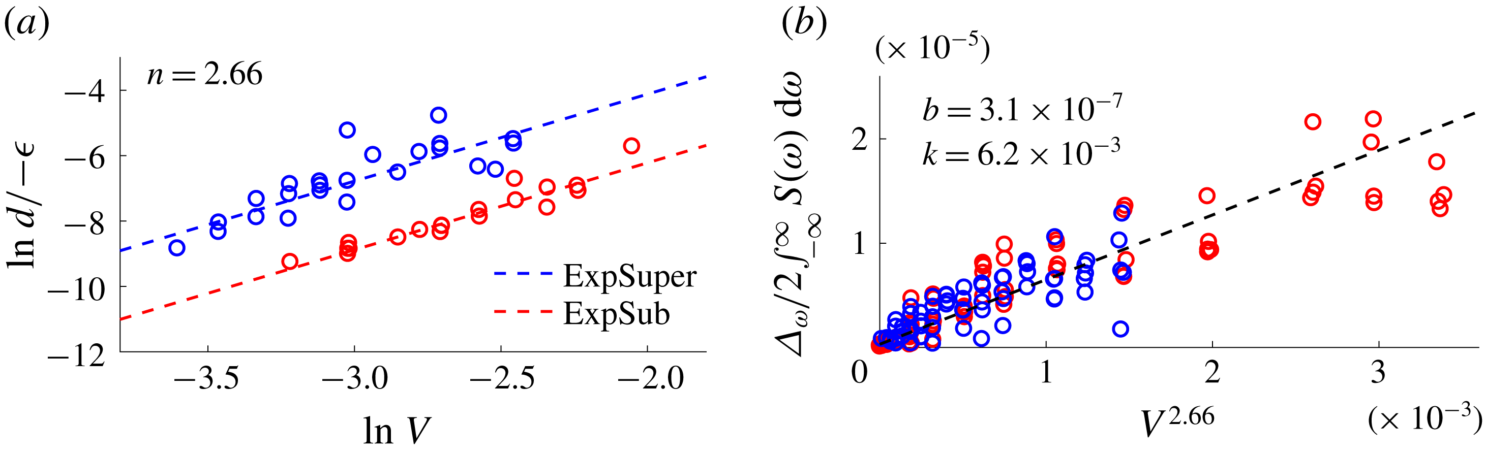
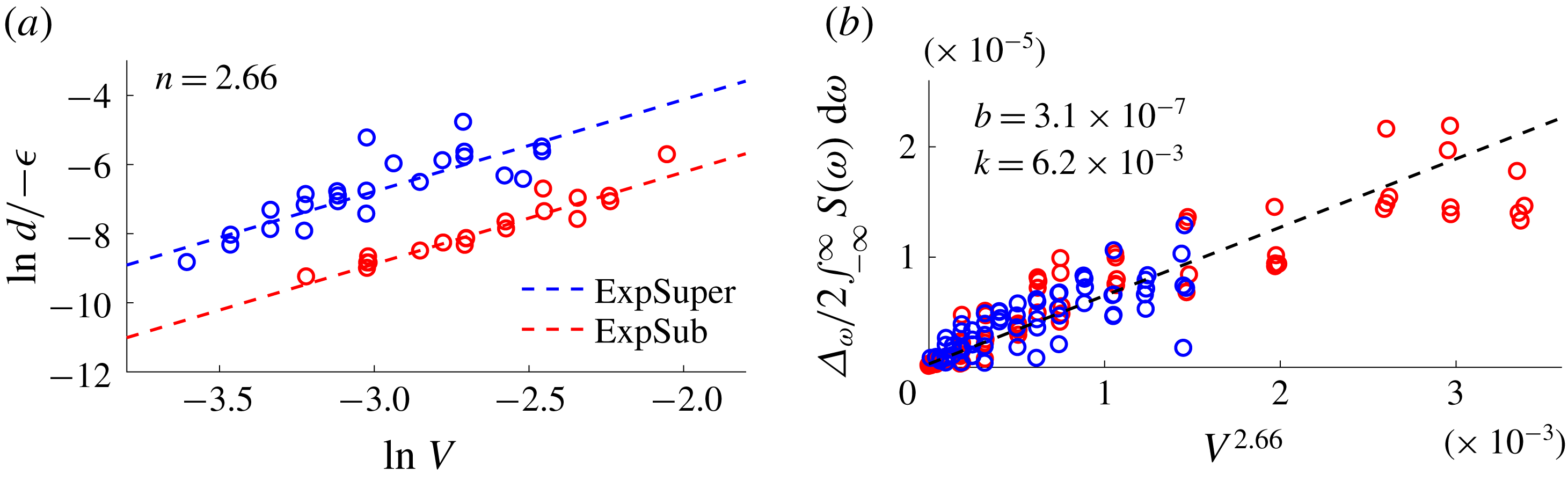
in figure 4(a). The data for both ExpSuper and ExpSub fit well with a common slope of
 $n=2.66$
. The
 $y$
-intercept directly gives
 $\ln (k/\!-\unicode[STIX]{x1D716})$
, but neither
 $k$
nor
 $\unicode[STIX]{x1D716}$
is known at this stage.
Modelling of the actuator to determine (a)
 $n$
and (b)
 $b$
and
 $k$
. The markers are experimental data, and the dotted lines are linear fits.
To find
 $k$
and
 $b$
, we use information in the spectral domain. Following Ushakov et al. (Reference Ushakov, Wünsche, Henneberger, Khovanov, Schimansky-Geier and Zaks2005), we derive an equation for the jet spectrum (
 $S_{u}$
):
 $$\begin{eqnarray}\int _{-\infty }^{\infty }S_{u}(\unicode[STIX]{x1D714})\,\text{d}\unicode[STIX]{x1D714}=\frac{2d}{\unicode[STIX]{x1D6E5}_{\unicode[STIX]{x1D714}}}=\frac{2(b+kV^{n})}{\unicode[STIX]{x1D6E5}_{\unicode[STIX]{x1D714}}},\end{eqnarray}$$
where
 $\unicode[STIX]{x1D6E5}_{\unicode[STIX]{x1D714}}$
is the half-width at half-maximum when a Lorentzian curve is fitted to
 $S_{u}$
. The coefficients
 $k$
and
 $b$
are then extracted from the
 $y$
-intercept and gradient of the data in figure 4(b), respectively. Thus, the relationship between the input loudspeaker voltage and the noise amplitude is
 $d=(3.1\times 10^{-7})+(6.2\times 10^{-3})V^{2.66}$
. The fact that data for both ExpSuper and ExpSub fit this power-law model and that
 $b$
is indeed very small justifies our modelling assumptions for the actuator.
3.3 System identification
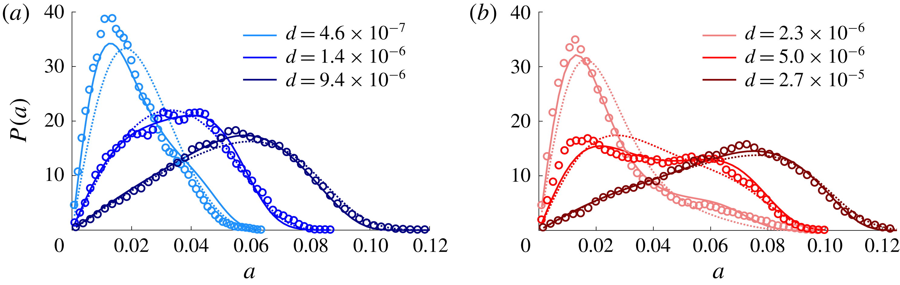
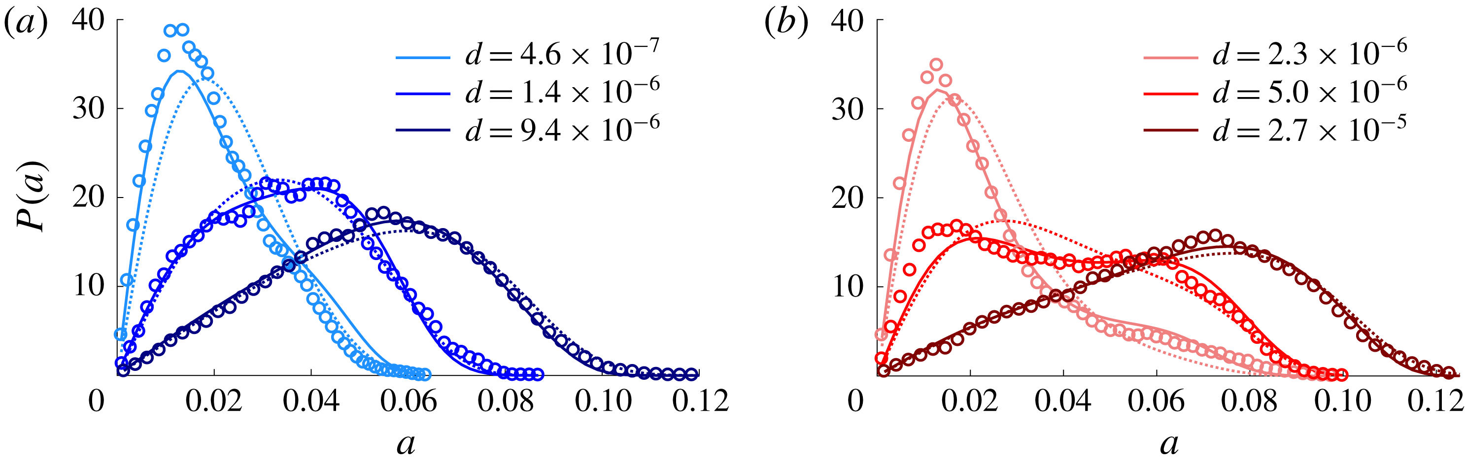
Figure 5 shows the probability density function of the velocity fluctuation amplitude,
 $P(a)$
, in the jet for (a) ExpSuper and (b) ExpSub under increasing noise amplitudes. The model coefficients (
 $\unicode[STIX]{x1D716}$
and
 $\unicode[STIX]{x1D6FC}_{1,\ldots }$
) are found by fitting polynomials to (3.8) with the measured
 $P(a)$
. More specifically, the model coefficients are found via a linear least-squares fitting solution of the following matrix problem:
 $$\begin{eqnarray}\left[\begin{array}{@{}c@{}}\ln P(a_{b1})-\ln a_{b1}\\ \ln P(a_{b2})-\ln a_{b2}\\ \vdots \\ \ln P(a_{bN})-\ln a_{bN}\end{array}\right]=\left[\begin{array}{@{}ccccc@{}}1 & a_{b1}^{2} & a_{b1}^{4} & a_{b1}^{6} & \cdots \\ 1 & a_{b2}^{2} & a_{b2}^{4} & a_{b2}^{6} & \cdots \\ \vdots & \vdots & \vdots & \vdots & \\ 1 & a_{bN}^{2} & a_{bN}^{4} & a_{bN}^{6} & \cdots \end{array}\right]\left[\begin{array}{@{}c@{}}\ln C\\ {\displaystyle \frac{\unicode[STIX]{x1D716}}{2d}}\\ {\displaystyle \frac{\unicode[STIX]{x1D6FC}_{1}}{16d}}\\ {\displaystyle \frac{\unicode[STIX]{x1D6FC}_{2}}{48d}}\\ \vdots \end{array}\right],\end{eqnarray}$$
where
 $a_{b1},a_{b2},\ldots ,a_{bN}$
are uniformly distributed bins of
 $a$
(i.e. the
 $x$
axis of figure 5). At each
 $Re$
, there are 20 and 19 different levels of
 $d$
in ExpSuper and ExpSub, respectively. For each value of
 $d$
, there are five sets of data. The final values of the model coefficients are determined by averaging across all levels and sets of
 $d$
at each
 $Re$
. In this averaging procedure, we exclude outliers by discarding the data points within 20 % of the extrema. Figure 5 shows that the ability of the model to reproduce
 $P(a)$
improves as the number of nonlinear terms in the model increases.
Probability density function
 $P(a)$
at different noise amplitudes for (a) ExpSuper (
 $Re=584$
) and (b) ExpSub (
 $Re=755$
). The markers are experimental data, and the dashed and solid lines are numerical estimates from the N5 model (up to
 $\unicode[STIX]{x1D6FC}_{2}$
, quintic order) and the N9 model (up to
 $\unicode[STIX]{x1D6FC}_{4}$
, nonic order), respectively.
4 Results and discussion
4.1 Determination of the order of nonlinearity
The order of nonlinearity in the system is determined based on the number of nonlinear terms required to reproduce the measured
 $P(a)$
. This is achieved by successively adding higher-order nonlinear terms to (3.1) until the rank of the matrix in (3.11) becomes deficient. Figure 5(b) shows that, at an intermediate noise amplitude, two peaks appear in
 $P(a)$
. This behaviour is called bimodality and is observed in both ExpSuper and ExpSub. We derive a condition for the amplitude (
 $a_{m}$
) at which extrema of
 $P(a)$
occur:
 $$\begin{eqnarray}d+\unicode[STIX]{x1D716}a_{m}^{2}+\frac{\unicode[STIX]{x1D6FC}_{1}}{4}a_{m}^{4}+\frac{\unicode[STIX]{x1D6FC}_{2}}{8}a_{m}^{6}+\frac{5\unicode[STIX]{x1D6FC}_{3}}{64}a_{m}^{8}+\frac{7\unicode[STIX]{x1D6FC}_{4}}{128}a_{m}^{10}+\cdots =0.\end{eqnarray}$$
For bimodality to exist, there must be two positive solutions of
 $a_{m}^{2}$
at some values of
 $d$
. For this to occur, the model must have nonlinear terms up to at least quintic order (
 $\unicode[STIX]{x1D6FC}_{2}$
).
To reproduce
 $P(a)$
, we show three different models. The first model, called N5, has up to fifth-order (quintic) nonlinearity, requiring up to
 $\unicode[STIX]{x1D6FC}_{2}$
, which is the minimum for bimodality. The second and third models have up to ninth-order (called N9; up to
 $\unicode[STIX]{x1D6FC}_{4}$
) and thirteenth-order (called N13; up to
 $\unicode[STIX]{x1D6FC}_{6}$
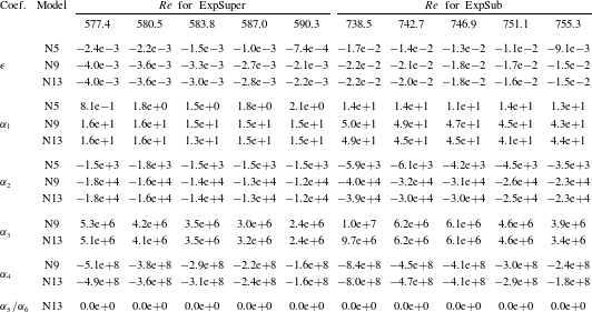
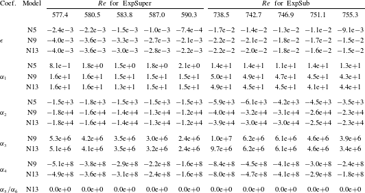
) nonlinearity, respectively. Table 1 lists the coefficients for the three models. It can be seen that when going from N5 to N9, the coefficients change significantly – by an order of magnitude in many cases. However, when going from N9 to N13, only a small change in the coefficients is observed, with
 $\unicode[STIX]{x1D6FC}_{5}$
and
 $\unicode[STIX]{x1D6FC}_{6}$
being negligible. In figure 5, we observe that the N9 model (solid lines) reproduces
 $P(a)$
satisfactorily. Thus, we conclude that the nonlinearity in this system is up to ninth order.
Model coefficients for ExpSub and ExpSuper. The models N5, N9 and N13 have up to
 $\unicode[STIX]{x1D6FC}_{2}$
,
 $\unicode[STIX]{x1D6FC}_{4}$
and
 $\unicode[STIX]{x1D6FC}_{6}$
terms, respectively. Increasing the order of nonlinearity above the nonic term (
 $\unicode[STIX]{x1D6FC}_{4}$
) does not further improve the agreement with the experimental data.
4.2 Prediction of dynamic and stochastic bifurcations
The main motivation for SI is to be able to predict dynamic bifurcations (i.e. the Hopf and saddle-node points) and, hence, the stability boundaries. In addition to this, we also predict stochastic P-bifurcations, i.e. when the system switches from unimodal to bimodal behaviour (Zakharova et al. Reference Zakharova, Vadivasova, Anishchenko, Koseska and Kurths2010). Stochastic P-bifurcations are important for determining the dynamic bifurcations of noisy systems (Zakharova et al. Reference Zakharova, Vadivasova, Anishchenko, Koseska and Kurths2010).
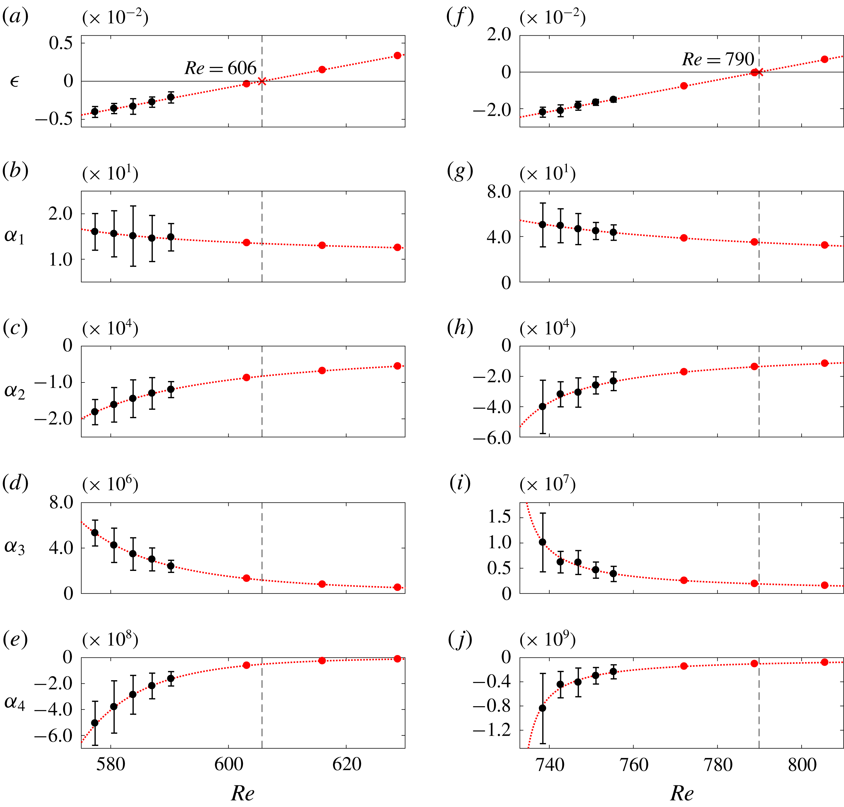
Model coefficients with respect to
 $Re$
for (a–e) ExpSuper and (f–j) ExpSub. The black markers with error bars are the experimental data. The dotted red lines are (a,f) linear fits and (b–e,g–j) power-law fits. The red markers are the extrapolated points for ExpSuper (
 $Re=603$
, 616, 629) and for ExpSub (
 $Re=772$
, 789, 806).
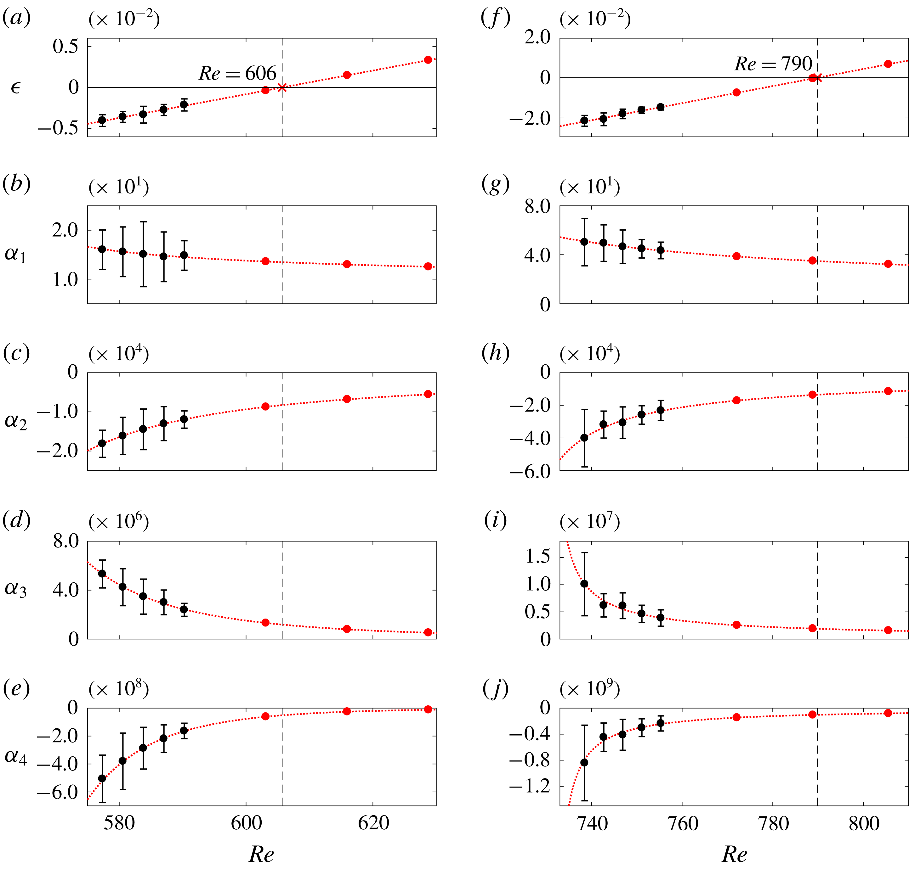
To predict the bifurcation points, we extrapolate the model coefficients calculated in § 4.1 to higher
 $Re$
, as shown in figure 6. We use a linear regression for
 $\unicode[STIX]{x1D716}$
, much as Provansal et al. (Reference Provansal, Mathis and Boyer1987) did in their experiments on a cylinder wake. For the higher-order coefficients, we use a power-law fit:
 $\unicode[STIX]{x1D6FC}_{n}\propto (Re-m_{1})^{-m_{2}}$
, where
 $m_{1}$
and
 $m_{2}$
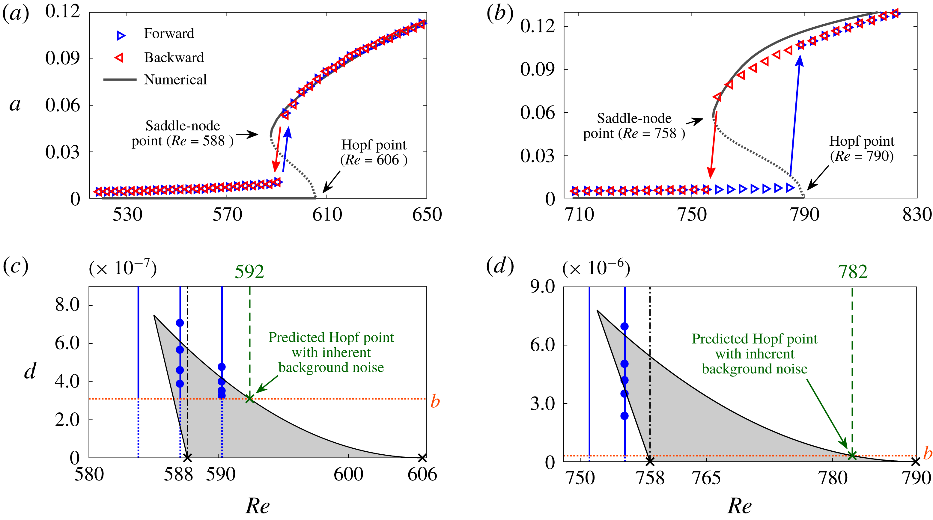
are positive constants obtained from least-squares fitting of the experimental data. From the extrapolated coefficients, we generate dynamic and stochastic bifurcation plots for ExpSuper and ExpSub, and compare them in figure 7 with our experimental data. The dynamic bifurcation plots are generated by solving (3.5a
) without the effect of noise, whereas the stochastic bifurcation plots are generated by finding solutions of (4.1) that have two positive
 $a_{m}^{2}$
.
Dynamic and P-bifurcation plots for (a,c) ExpSuper and (b,d) ExpSub. In (a,b), the solid and dotted lines denote the stable and unstable solutions, respectively, as calculated from the model. In (c,d), the grey areas denote the bimodal regime calculated from the model, the blue vertical lines denote where the experiments were conducted and the blue circular markers denote where bimodality is observed experimentally. The orange horizontal lines denote the inherent amplitude of the background noise.
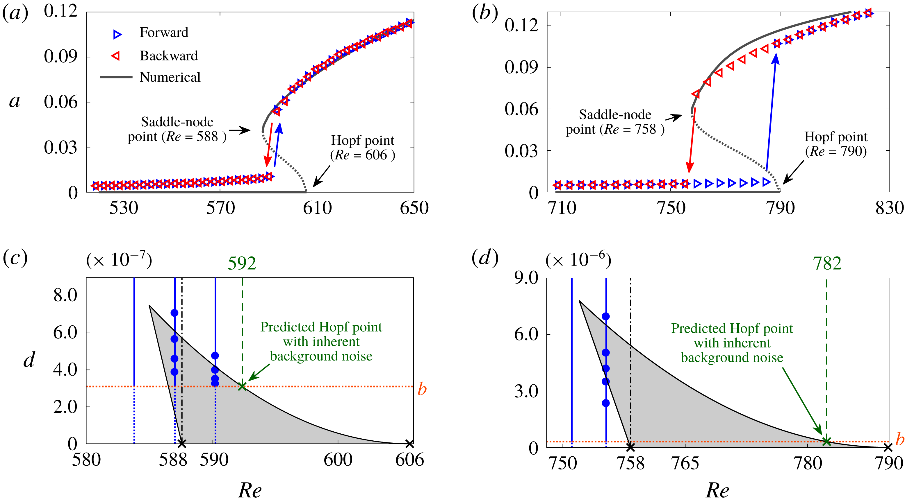
Figure 7(a,b) shows that, without noise (
 $d=0$
), the numerically predicted Hopf and saddle-node points are, respectively, at
 $Re=606$
and 588 for ExpSuper, and at
 $Re=790$
and 758 for ExpSub. The model correctly identifies ExpSub to be subcritical but, curiously, it identifies ExpSuper to be subcritical as well, which might seem to contradict the experiments. However, a careful examination of the experimental data (figure 7
a) shows a marked jump in the oscillation amplitude at the bifurcation point. We speculate that this jump occurs because the Hopf and saddle-node points have either collided or moved so close to each other as to be indistinguishable within the limits of experimental uncertainty. This interpretation of supercritical-like behaviour can also explain previous observations of a similar amplitude jump in the low-density jet experiments of Hallberg & Strykowski (Reference Hallberg and Strykowski2006) and Zhu et al. (Reference Zhu, Gupta and Li2017). Moreover, the presence of background noise shrinks the hysteretic bistable region by triggering LCOs. Next, we examine the effect of background noise on dynamic bifurcations using P-bifurcation plots.
Bimodality is usually associated with subcritical Hopf bifurcations (Zakharova et al.
Reference Zakharova, Vadivasova, Anishchenko, Koseska and Kurths2010). As shown in figure 7(c,d), bimodality (grey areas) exists between the Hopf and saddle-node points, even for infinitesimally weak noise. Bimodality represents the tendency of a system to switch between the zero-amplitude state and the LCO state in the bistable regime. In the presence of finite-amplitude noise, this tendency can be observed even before the system reaches the saddle-node point. This is seen in our experiments (figure 7
c,d: blue markers) and is well predicted by our model. Background noise, however, can shrink the bimodal region by triggering LCOs. In figure 7(c,d), this shrinkage can be seen as a tapering of the bimodal region (grey area) above the inherent amplitude of the background noise,
 $b$
(orange horizontal line). Therefore, for an accurate comparison between the predicted and experimentally observed bifurcation points, we must account for the effect of noise. We do this by locating the points (green crosses) at which
 $b$
(orange horizontal line) intersects the bimodal region (grey area). For ExpSuper (figure 7
c), this gives a predicted Hopf point of
 $Re=592$
, which matches exactly with the experimentally observed value at
 $Re=592$
(figure 2
a). As mentioned earlier, the absence of a bistable region can be understood because it is exceedingly small. For ExpSub (figure 7
d), the intersection of
 $b$
and the bimodal region gives predicted Hopf and saddle-node points of
 $Re=782$
and 758, respectively, which match well with the experimentally observed values at
 $Re=787$
and 757 (figure 2
b).
4.3 Prediction of the system dynamics beyond the bifurcation points
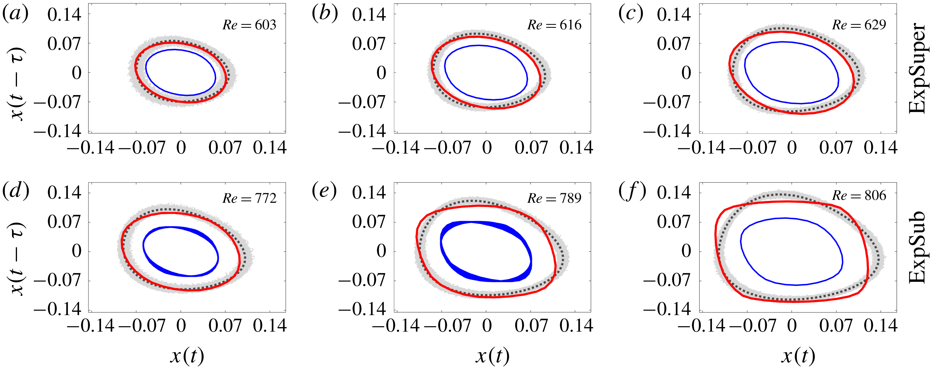
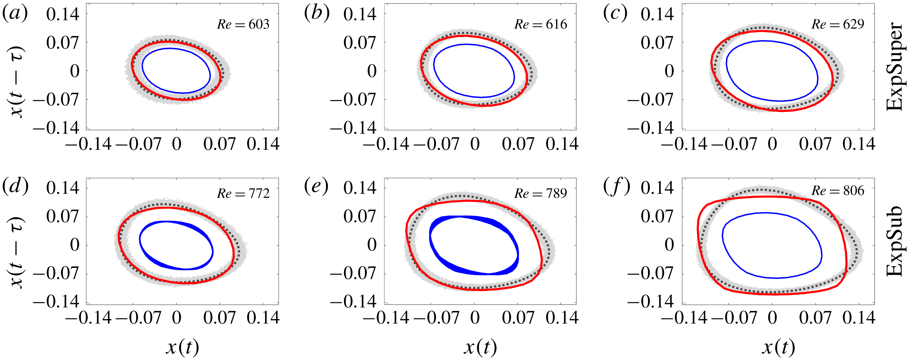
We now turn to predicting the system dynamics away from the bifurcation points. Figure 8 shows phase portraits of the LCOs for (a–c) ExpSuper at
 $Re=603$
, 616 and 629, and (d–f) ExpSub at
 $Re=772$
, 789 and 806. These are compared with the corresponding LCOs from the experiments. In seminal work, Takens (Reference Takens1981) showed that the dynamical properties of a system containing many degrees of freedom can be represented by just a single scalar time series with an appropriately chosen time delay (
 $\unicode[STIX]{x1D70F}$
). Here, we show the phase portrait in two dimensions with
 $\unicode[STIX]{x1D70F}$
calculated using the average mutual information method of Fraser & Swinney (Reference Fraser and Swinney1986). The comparison between the experimental and numerical LCOs shows that the N9 model can accurately predict both the amplitude and shape of the LCO orbits. This further highlights the important role that the higher-order nonlinear terms have in determining the system dynamics.
Phase portraits of the LCOs for (a–c) ExpSuper and (d–f) ExpSub. The experimental LCO orbits (grey bands) are shown alongside their mean orbits (black dotted lines). These can be compared with the numerically obtained LCO orbits from the N5 model (blue line) and the N9 model (red line).
5 Conclusions
We perform SI of a low-density jet from its noise-induced dynamics, using a low-order oscillator model and its corresponding Fokker–Planck equation. To the best of our knowledge, this is the first time that SI has been achieved on an experimental system using the noise-induced dynamics in only the unconditionally stable regime, i.e. without having to operate in the regimes where LCOs may occur. We show that our estimated numerical model can accurately predict three key system properties: (i) the order of nonlinearity, (ii) the locations and types of the bifurcation points (and hence the stability boundaries) and (iii) the limit-cycle dynamics beyond the bifurcation points.
There are two main implications of this work that go beyond low-density jets. First, the SI methodology proposed here should be applicable to many other dynamical systems, as the only inherent assumption made about the system is that it obeys the Stuart–Landau equation. This assumption is, in fact, valid in the vicinity of the Hopf point for many dynamical systems – hydrodynamic or otherwise. Consequently, the Stuart–Landau equation has been used in a number of other SI methodologies in the literature (see § 1). However, in all of those studies, it has been assumed that the nonlinear terms can only be obtained from data collected during the occurrence of LCOs, in the unstable or bistable regime. With our SI methodology, however, we show that data from the noise-induced dynamics in the unconditionally stable regime are themselves enough to determine the bifurcation points and to predict the LCO dynamics beyond those points. Thus, our SI methodology opens up new pathways for the development of early-warning indicators and active-control strategies against unwanted oscillations in systems operating near a Hopf point. This is particularly useful for the design of systems prone to exhibiting dangerously energetic LCOs, such as thermoacoustic oscillations in gas turbines and rocket engines.
Second, the prediction of system nonlinearity – in particular, the order and signs of the nonlinear terms – can provide physical insight into the system. For plane Poiseuille flow, Stuart (Reference Stuart1960) was able to explain that the physical meaning of a positive
 $k_{2}$
term is that the distortion of the fundamental instability mode is dominant over the combination of the distortion of the mean motion and the generation of harmonics. It is beyond the scope of this paper to perform an equivalent analysis for the low-density jet and extend it to the higher-order terms. Stuart (Reference Stuart1960), however, did not attempt to calculate the nonlinear terms, which we have done here.
As for improvements to this SI methodology, we should be able to relax the assumption that the background noise amplitude is small. In many natural and engineered systems, background noise can be significant, making the development of an actuator model difficult. An instinctive solution is to turn to output-only SI methods, but these are usually only reliable when the input data size is large (Mevel et al. Reference Mevel, Benveniste, Basseville, Goursat, Peeters, Van der Auweraer and Vecchio2006). This problem can be alleviated through the use of adjoint equations, as demonstrated by Boujo & Noiray (Reference Boujo and Noiray2017). Furthermore, in the simple axisymmetric jet studied here, we have used information collected at only one spatial location. This keeps the system size small without adversely affecting the quality of the predictions for the bifurcation points and LCO dynamics. However, there could be other, more complicated, flows for which it may be useful to include information about the spatial structure of the global instability mode. In such cases, we may need to incorporate the use of sparsity-promoting tools and machine learning in this SI framework to deal with the larger data matrices.
Acknowledgements
This work was funded by the Research Grants Council of Hong Kong (Project Nos 16235716 and 26202815). V.G. was supported by the National Natural Science Foundation of China (grant no. 11672123) and by the Shenzhen Science and Technology Program (grant no. JCYJ20170412151759222). M.L. was supported by the Hong Kong PhD Fellowship Scheme.