Introduction
The introduction and spread of invasive non-native species (INNS) has a dominant and wide-ranging impact on ecosystems and economies (He and Silliman, Reference He and Silliman2019; IPBES, Reference In Roy, Pauchard, Stoett and Renard Truong2023). Globally, approximately 200 new non-native species (NNS) are recorded annually (IPBES, Reference In Roy, Pauchard, Stoett and Renard Truong2023); however, not all NNS become invasive (i.e., problematic) (Williamson and Fitter, Reference Williamson and Fitter1996). Once introduced, an NNS population may establish (survive and reproduce for multiple generations), grow (in abundance), and spread (disperse to new sites from the site of introduction). Over time, distribution and abundance may increase exponentially, causing negative impacts due to the species becoming widespread and highly abundant (the species is now invasive) (Blackburn et al., Reference Blackburn, Pyšek, Bacher, Carlton, Duncan, Jarošík, Wilson and Richardson2011). These stages of the Invasion Process, which are not fully explicit and can therefore be categorised in various ways (e.g., Blackburn et al., Reference Blackburn, Pyšek, Bacher, Carlton, Duncan, Jarošík, Wilson and Richardson2011; Crooks, Reference Crooks2005; Williamson and Fitter, Reference Williamson and Fitter1996), will be termed introduction, establishment, growth, spread, and invasive impact for the purpose of this study. Understanding where an NNS lies within this process helps to determine whether it is, or is likely to become, invasive (Sakai et al., Reference Sakai, Allendorf, Holt, Lodge, Molofsky, With, Cabin, Cohen, Norman, McCauley, O’Neil, Parker, Thompson and Weller2001) – particularly in relation to density-dependant impacts such as resource competition – and also helps to optimise management (see the Invasion Curve; Victorian Government, 2010).
The transition of an NNS through the Invasion Process after initial introduction can take years or decades, and is notoriously difficult to predict, with time lags potentially occurring at each stage, and initial dates of introduction being hard to determine (Crooks, Reference Crooks2005). Common causes of lags include the exponential nature of population growth, biotic interactions, and the time required for sufficient propagule pressure and genetic variance to accumulate, and for evolutionary processes to occur (Crooks, Reference Crooks2005; Roman and Darling, Reference Roman and Darling2007; Sakai et al., Reference Sakai, Allendorf, Holt, Lodge, Molofsky, With, Cabin, Cohen, Norman, McCauley, O’Neil, Parker, Thompson and Weller2001). While identifying such lags and causal factors can be challenging (Crooks, Reference Crooks2005), population parameters can serve as indicators of environmental suitability, and the potential for population growth, spread, and invasive impact.
The Asian date mussel (Arcuatula senhousia) is an NNS of the intertidal and subtidal zones across the globe (maximum depth tolerance = 20 m; Kuroda et al., Reference Kuroda, Habe and Oyama1971). The native range of A. senhousia extends from Singapore northwards to Siberia (Chuang, Reference Chuang1961; Kulikova, Reference Kulikova1978). Its introduced range has become similarly extensive since the first reported introduction event on the Pacific coast of North America in the 1920s (Dexter, Reference Dexter1983); A. senhousia is now present in Oceania (Willan, Reference Willan1985, Reference Willan1987) and Africa (Lourenço et al., Reference Lourenço, Henriques, Catry, Pedro and Catry2018). In the 1980s, Hoenselaar and Hoenselaar (Reference Hoenselaar and Hoenselaar1989) reported A. senhousia from Europe for the first time, in the Western Mediterranean Sea ecoregion (ICES, 2025). In Northern Europe, the earliest record for A. senhousia was from 2002, from Arcachon Bay in France (Bachelet et al., Reference Bachelet, Blanchet, Cottet, Dang, Montaudouin, Moura Queirós, Gouillieux and Lavesque2009). Subsequently, A. senhousia has been recorded in the UK (first record in 2011, from the Solent) (Watson et al., Reference Watson, Dyos, Barfield, Stebbing and Dey2021; Worsfold et al., Reference Worsfold, Pennisi and Ashelby2020) and the Netherlands (first record in 2017, from Goese Meer; Faasse, Reference Faasse2018). Currently, A. senhousia is at relatively low densities of typically <100 ind. m−2 in Northern Europe (Bachelet et al., Reference Bachelet, Blanchet, Cottet, Dang, Montaudouin, Moura Queirós, Gouillieux and Lavesque2009; Faasse, Reference Faasse2018; Massé et al., Reference Massé, Jourde, Fichet, Sauriau, Dartois, Ghillebaert and Dancie2022; Watson et al., Reference Watson, Dyos, Barfield, Stebbing and Dey2021), although densities have reached >10,000 ind. m−2 in other parts of the globe, including temperate regions such as New Zealand (Creese et al., Reference Creese, Hooker, Luca and Wharton1997). In areas where A. senhousia has been recorded as invasive due to impacts on benthic community composition and resource competition, populations typically exceed densities of >1,000 ind. m−2, with conspecifics joining via byssal threads to form ‘mats’ (in New Zealand [Creese et al., Reference Creese, Hooker, Luca and Wharton1997], USA [Crooks, Reference Crooks1998; Crooks and Khim, Reference Crooks and Khim1999], and Italy [Como et al., Reference Como, Pais, Saba, Sprovieri and Magni2016; Mistri, Reference Mistri2002; Munari, Reference Munari2008]).
High population densities result from high individual fecundity, particularly for short-lived ephemeral species such as A. senhousia which typically lives for one year, although reported lifespans range from nine months (Morton, Reference Morton1974) to 17 or 18 months (Crooks, Reference Crooks1996; George and Nair, Reference George and Nair1974) and up to two years (Crooks, Reference Crooks1996). Living into a second year likely increases the chance of successful spawning and recruitment (Morton, Reference Morton1989), thereby facilitating higher fecundity, densities, and likelihood of invasive impact. Growth rate is similarly variable, with estimates ranging from 8 mm (Bachelet et al., Reference Bachelet, Blanchet, Cottet, Dang, Montaudouin, Moura Queirós, Gouillieux and Lavesque2009) to 25 mm (Crooks, Reference Crooks1996) per year. Faster growth may reduce time taken to reach sexual maturity and so, like a longer lifespan, increase individual – and by extension population – fecundity. Reported variation in bivalve spawning and recruitment is largely influenced by water chemistry, including temperature, chlorophyll levels (i.e., food availability), and salinity (e.g., Feng and Papeş, Reference Feng and Papeş2017; Liang et al., Reference Liang, Kim, Zhang, Lim and Kang2009; Sarà et al., Reference Sarà, Romano, Widdows and Staff2008; Sgro et al., Reference Sgro, Turolla, Rossi and Mistri2002; Verween et al., Reference Verween, Vincx and Degraer2007). Substrate type and availability also influence density. Arcuatula senhousia can attach to hard substrates, although higher densities of A. senhousia are typically associated with fine sediment (Crooks, Reference Crooks1996; Mistri, Reference Mistri2002; Morton, Reference Morton1974; Willan, Reference Willan1987) and the presence of filamentous or fibrous settlement substrate such as vegetation (Kikuchi, Reference Kikuchi1964; Kulikova, Reference Kulikova1978). These environmental factors vary temporally and spatially; consequently, so too does the invasive potential of NNS such as A. senhousia.
In Northern Europe, the reproductive cycle, growth rate, and lifespan of A. senhousia have been assessed to varying degrees, though by a limited number of studies and not all for the same population/location over the same time period (Bachelet et al., Reference Bachelet, Blanchet, Cottet, Dang, Montaudouin, Moura Queirós, Gouillieux and Lavesque2009; Faasse, Reference Faasse2018; Massé et al., Reference Massé, Jourde, Fichet, Sauriau, Dartois, Ghillebaert and Dancie2022; Watson et al., Reference Watson, Dyos, Barfield, Stebbing and Dey2021). Furthermore, the spatial and temporal variation of influential environmental variables limits the confidence that can be assigned to estimates of invasion stage. Therefore, the primary aim of this study was to determine the current invasion stage and potential future impact of A. senhousia in Northern Europe by assessing all aforementioned population parameters from the same population, during the same timeframe.
The A. senhousia population in the Solent, UK, was selected as an ideal study population due to evidence of self-sustaining and persistent populations, indicating a potential INNS risk (Watson et al., Reference Watson, Dyos, Barfield, Stebbing and Dey2021). Arcuatula senhousia’s population dynamics (density, individual lifespan and growth rate) and reproductive cycle (spawning and recruitment) were assessed through sampling conducted using a scientific dredge (from April 2021 to March 2022). Analysis included length-frequency distribution (LFD), electronic length-frequency analysis (ELEFAN), gonadosomatic index (GSI), condition index (CI), and histology. To support the interpretation of results, environmental variables were also assessed: sonar scan data (to assess water depth, vegetation presence/type, and sediment type) and drop-down camera data (to assess vegetation presence/type and A. senhousia distribution) obtained for this study; sediment particle size data (to assess sediment type) collected by the Environment Agency (EA) prior to the study period; and water chemistry data (to assess sea surface temperature, salinity and chlorophyll) collected by the EA during the study period.
The second aim of this study was to determine whether A. senhousia spawning in the Solent occurs outside of the June to October period identified by Watson et al. (Reference Watson, Dyos, Barfield, Stebbing and Dey2021), whose sampling was limited to March (early spring) through to October (early autumn). Prolonged spawning periods – whether single, extended or consisting of multiple events – are common across multiple bivalve species and reflect their capacity to adapt reproductive cycles to environmental conditions (Gosling, Reference Gosling2003a).
Materials and methods
Population dynamics and reproductive cycle
Specimens of A. senhousia were obtained from Southampton Water, an estuary on the south coast of England (50°50′52″N, 1°19′42″W) which hosts the Port of Southampton and multiple passenger ferry terminals and is lined by industrial and residential developments (Figure 1). The specimen collection site was within the River Test (one of the main freshwater inputs to Southampton Water), in an area of 0.08 km2 (1.7 km perimeter) which lies adjacent to a shipping channel (Figure 1). This location was selected based on prior records indicating the presence of A. senhousia in the area (Watson et al., Reference Watson, Dyos, Barfield, Stebbing and Dey2021).
Southampton Water, in the Solent region on the south coast of England, showing: i) the specimen collection area where dredging was carried out and a sonar scan was conducted to assess water depth, vegetation presence/type, and sediment type; ii) the area where a drop-down camera survey was conducted to assess vegetation presence/type and Arcuatula senhousia distribution; iii) the location where water samples were taken by the Environment Agency (EA) to assess sea surface temperature, chlorophyll, and salinity. Satellite image depicts a mix of residential, industrial, and agricultural land use. Satellite image: Map Data © 2025 Google.

Specimens were collected in April, June, July, October and November 2021, and January and March 2022 (one sampling trip per month), using a 60 × 20 cm dredge with a 5 mm mesh. A mean length of 1.8 km (0.001 km2) was dredged each month, consisting of four to five separate tracks. Dredged material was sieved with 5 mm mesh in a laboratory, within 2–3 hours of collection, to extract specimens. Journey time from the specimen collection site to the laboratory was 2–3 hours. Extracted specimens were placed in 40 L tanks with a continuous flow of harbour water until specimen processing (dissection or fixation), which occurred within 2–3 days.
Mean monthly population density was calculated as the mean density per dredge track. These values are relative estimates due to the low-resolution data, resulting from the extended track lengths and potential specimen loss through the 5 mm mesh. For April, population density was calculated by dividing the total number of specimens collected by the total area dredged, since track numbers were not recorded that month.
Gonadosomatic index and condition index
Both GSI and histology were used to determine the reproductive cycle due to their respective advantages and limitations (Brewer et al., Reference Brewer, Rabeni and Papoulias2008; Ojea et al., Reference Ojea, Pazos, Martínez, Novoa, Sánchez and Abad2004). CI was also assessed in combination with GSI and histological analysis, since it is considered a sensitive index for determining the reproductive cycle of bivalves (Ojea et al., Reference Ojea, Pazos, Martínez, Novoa, Sánchez and Abad2004; Peharda et al., Reference Peharda, Mladineo, Bolotin, Kekez and Skaramuca2006). In each sampling month, 20–40 specimens with a shell length (SL) of at least 16 mm (i.e., specimens of reproductive age; Sgro et al., Reference Sgro, Turolla, Rossi and Mistri2002) were randomly selected from all specimens extracted from the dredged material. The same specimens were used for GSI and CI analyses. Their adductor muscles were cut before they were placed in 70% ethanol and dissected 1-4 weeks later. Total tissue and gonad tissue was weighed to the nearest 1 mg. Each specimen’s tissue and shell were dried in an oven at 60°C for 24 hours, then weighed to the nearest 1 mg. GSI and CI were calculated using standard equations (Siah et al., Reference Siah, Pellerin, Amiard, Pelletier and Viglino2003; Walne, Reference Walne1976, respectively).
Gonad index and gonad stage
Each sampling month, 10–20 specimens were placed in sample pots containing 40 mL of Bouin’s fixative for 3 days, with pots inverted at least once daily. Specimens were fixed whole (shell and tissue) due to their small size (20–30 mm), reducing the risk of tissue damage during dissection (Kim et al., Reference Kim, Ashton-Alcox and Powell2006). After fixation, 5 mm cross-sections were cut using a scalpel and placed in 70% ethanol for 1–7 days before tissue embedding using standard procedures (Howard et al., Reference Howard, Lewis, Keller and Smith2004; Kim et al., Reference Kim, Ashton-Alcox and Powell2006). After sectioning, tissue was stained with Haematoxylin and Eosin (H&E). Specimens collected in April were stained using Clin-Tech’s H&E rapid staining kit (catalogue number 631210); however, due to difficulties obtaining more of this product, all other specimens were stained with Abcam’s H&E staining kit (product number ab245880). Stained tissues were assessed by scanning the microscope slides using an Olympus VS200 Research Slide Scanner and visualising the resulting images with OlyVIA software (Ver. 2.9.1). Gonad tissue was categorised into one of four reproductive stages – resting, developing, ripe, or spawning – and assigned a numerical stage (Seed, Reference Seed1969). The mean GI was calculated for each sampling month using the standard equation (Bayne, Reference Bayne1976). GI values range from zero, when the entire population is resting, to five when fully ripe (Bayne, Reference Bayne1976).
Length-frequency distribution and growth rate
Length-frequency distribution graphs were used to analyse both population dynamics and the reproductive cycle. The SLs of all specimens were measured using callipers to an accuracy of 0.5 mm. SL was measured as the maximum dimension across the shell, taken perpendicular to the hinge line (Gosling, Reference Gosling2003b). Histograms and kernel density plots were used to assess whether the populations were uni- or bimodal. In April, the relatively small sample size (n = 31) made it difficult to distinguish how many cohorts were present, so the excess mass test was applied (testing the null hypothesis that the true number of modes is >1) using the ‘modetest’ function in the ‘multimode’ library in R (Ameijeiras-Alonso et al., Reference Ameijeiras-Alonso, Crujeiras and Rodriguez-Casal2021). The mode of each age group (hereafter referred to as cohort) in months with a unimodal distribution (April and June) was identified by using the ‘mlv’ function (method = ‘Parzen’) in the ‘modeest’ R package (Poncet, Reference Poncet2019). For months with a bimodal distribution (July, October, November, January, March) cohort modes were identified using the ‘locmodes’ function of the ‘multimode’ R package (Ameijeiras-Alonso et al., Reference Ameijeiras-Alonso, Crujeiras and Rodriguez-Casal2021). Both functions calculate modes based on the kernel density estimate.
The length-frequency dataset for A. senhousia was analysed using the ELEFAN method, implemented via the ‘ELEFAN’ function in the ‘TropFishR’ R package (Mildenberger et al., Reference Mildenberger, Taylor and Wolff2017). This approach fits a growth curve based on the von Bertalanffy growth function, allowing estimation of growth parameters from observed size distributions. Length-frequency data were plotted for each sampling month using different bin sizes until cohorts could be clearly distinguished, resulting in a bin size of 1 (i.e., 1 mm). The parameter MA (the number of length classes over which the moving average is performed) was selected by approximating the number of bins spanning the smallest (i.e., youngest) cohort width, resulting in MA = 11. Given a bin size of 1, MA = 11 corresponds to averaging over 11 adjacent bins, which spans a total length of 11 mm. A square root transformation was applied to the frequency counts to enhance cohort detection. Asymptotic length was calculated using the Powell–Wetherall method (‘Powell-Wetherall’ function in the ‘TropFishR’ R package; Mildenberger et al., Reference Mildenberger, Taylor and Wolff2017), resulting in an estimated length of 35 mm. The R command used for this analysis was ELEFAN (lengthfrequencydata, agemax = 2, MA = 11, addl.sqrt = TRUE, method = ‘optimise’, Linf_fix = 35).
Water chemistry and physical environment
Environmental data in and around the specimen collection site (Figure 1) were recorded, and data collected by the EA were analysed, to explore the potential drivers of the reproductive cycle and population dynamics. Sea surface temperature, chlorophyll, and salinity data were downloaded from the EA’s online Water Quality Archive (Environment Agency, 2023) for April 2021 to March 2022 and plotted. These data had been collected approximately 0.8 km northwest of the specimen collection site (Figure 1), comprising one sample per month (n = 12). To determine substrate type at the specimen collection site and the surrounding area (within 3 km), particle size data for Southampton Water were obtained from the EA via email correspondence. These data were collected in 2011 (n = 3 samples), 2013 (n = 4 samples), and 2016 (n = 2 samples) as part of routine monitoring for the Water Framework Directive (WFD). Sediment type was determined by calculating a mean particle size for each sample and matching it to the corresponding Wentworth Size Class (Wentworth, Reference Wentworth1922). Additionally, water depth, vegetation presence and type, and sediment hardness at the specimen collection site were assessed via a sonar scan of the entire site conducted on 16 August 2022 for this study and plotted. On the same day, the distribution and patchiness of A. senhousia, as well as vegetation presence and type within the dredge sampling area, were assessed using a drop-down camera survey (n = 64 samples). Methods for the sonar scan and drop-down camera survey are detailed in Supplementary Material: SM1.
Results
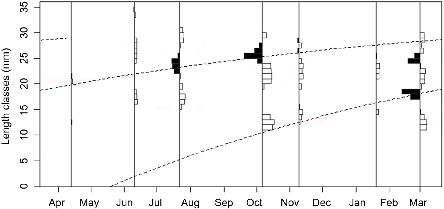
A total of 1,029 specimens were collected via dredging. Per sampling month, the numbers of specimens collected ranged from 31 to 283, and mean population density ranged from 0.05 to 0.5 individuals per m2 (ind. m−2). Mean dredged track length was 435 m (range: 165–824 m; SD = ± 198). SL ranged from 6.5 to 29.0 mm (mean = 20.6 mm; ±4.2 SD). ELEFAN determined a growth coefficient (K) of 0.93 and predicted that A. senhousia grew to 22 mm in length during the first year, with an average monthly growth rate of 1.8 mm (Figure 2). Growth slowed over time, with individuals growing an additional 6 mm if they lived into a second year (Figure 2). Based on the mean SL of 20.6 mm and the ELEFAN-derived growth curve, the mean lifespan was estimated at 11 months. The maximum lifespan, based on the maximum recorded SL of 29 mm, and the growth curve, was 23 months (Figure 2).
Reconstructed length-frequency distribution with growth curves, using Electronic Length Frequency Analysis (ELEFAN) (L∞ = 35 cm, K = 0.93 year−1) based on Arcuatula senhousia shell length (SL) data collected from April 2021 to March 2022. The black and white bars are positive and negative deviations from the moving average. Solid lines indicate the position within the month that sampling was carried out. Dashed lines link successive peaks of growing cohorts as extrapolated by the model, forming the growth curve, representing the growth of an individual in the population.

Seasonal changes in population dynamics and reproduction
Two age cohorts were apparent throughout much of the sampling year (July 2021 to March 2022), indicated by a bimodal distribution of SL data. The first and second cohorts detected were termed Cohort 1 (C-1) and Cohort 2 (C-2), respectively (Figure 3). Developing gonad tissue was observed in specimens from every sampling month (Figure 4), although marked seasonal changes in reproductive status and population dynamics were evident. Specimen collection began in April 2021, when only C-1 was present, and the data distribution was unimodal (excess mass = 0.10; p = 0.54) with a modal SL of 18.0 mm (Figure 3). Assuming a mean growth rate of 1.8 mm per month during the first year, specimens collected in April 2021 likely originated from a spawning event the year before, in June 2020 (18.0 mm ÷ 1.8 mm = ∼ 10 months prior). Population density was lowest in April 2021, at 0.04 ind. m−2 (n = 31).
Length-frequency histograms (grey columns) and kernel density plots (overlaid black solid lines) for Arcuatula senhousia collected from April 2021 to March 2022. Shell length (SL) modes of the first cohort to become apparent (C-1) are shown in light grey circles (with dotted outline), shell length modes of the second cohort to become apparent (C-2) are shown in dark grey circles (with solid outline).

The condition index (A), gonadosomatic index (B) gonad index (C) and gonad stage (D) of a subtidal Arcuatula senhousia population in the UK, from April 2021 to March 2022 (data were collected in April, June, July, October, November, January, and March). Also, (E) displays the mean density of individuals per m2 (ind. m-2) and (F) displays the sea surface salinity (ppt), temperature (°C) and chlorophyll (µg/l) data collected from April 2021 to March 2022 by the Environment Agency (EA) (see sample location in Figure 1).

After April 2021, the modal SL of C-1 increased, peaking at 23.4 mm in July 2021 (Figure 3). In July, a second cohort was also apparent (C-2), with a modal SL of 14 mm (before July 2021, only two A. senhousia specimens with an SL <14 mm were detected: 12.5 mm SL in April 2021, and 12 mm SL in June 2021) (Figure 3). Based on the growth rate, C-2 specimens collected in July 2021 likely resulted from a spawning event the year before, in November 2020 (14 mm ÷ 1.8 mm = ∼ 7.8 months prior). CI, GSI, and GI had increased markedly from April 2021 and peaked in June 2021 (mean = 20.8, 28.6 and 4.4, respectively) when the highest percentage of ripe gonad tissue was recorded (9/20 specimens = 45%) (Figure 4; see histology images in Supplementary Material: SM2). Sea surface temperature and chlorophyll also peaked in June 2021 and July 2021, respectively (see Water Chemistry section) (Figure 4). Population density had increased by a factor of 2.0 from April to June 2021 (reaching 0.08 ind. m−2; n = 158), and by a further factor of 3.9 from June to July 2021 (reaching 0.31 ind. m−2; n = 174) (Figure 4).
After July 2021, the modal SL of C-1 continued to increase, reaching 28.3 mm in November 2021. In contrast, C-2 growth was minimal for the rest of the specimen collection period, with modal SL reaching 17.1 mm by October 2021 and 17.2 mm by March 2022 (Figure 3). By October 2021, population density had increased by a factor of 1.6 since July 2021 (reaching 0.50 ind. m−2; n = 283) – the highest recorded since April 2021 – but decreased markedly by a factor of 0.1 (reaching 0.06 ind. m−2; n = 80) by November 2021 (Figure 4). CI, GSI, and GI had also decreased markedly by October 2021 (mean = 8.4, 15.4, and 2.0, respectively), although GI increased by November 2021 (mean = 2.6) (Figure 4). Similarly, sea surface temperature and chlorophyll had decreased by October 2021 and remained low for the rest of the specimen collection period (see Water Chemistry section; Figure 4). Spawning gonad tissue was detected for the first time in November 2021 (3/10 specimens = 30%), while CI remained low (mean = 8.0) and GSI continued to decline (mean = 9.1; Figure 4).
From November 2022 to January 2022, the modal SL of C-1 decreased to 24.4 mm (Figure 3), and population density decreased by a factor of 0.8, to 0.05 ind. m−2 (n = 71) – the lowest since April 2021. By January 2022, CI remained low (mean = 8.1), GSI had decreased (mean = 5.1), GI had decreased (mean = 1.6), and spawning gonad tissue was no longer detected. Only developing (6/9 specimens = 66%) and resting (3/9 specimens = 33%) gonad tissue were observed (Figure 4). From January 2022 to March 2022, the modal SL of C-2 decreased to 23.7 mm (Figure 3), while population density increased by a factor of 3.8 (reaching 0.19 ind. m−2; n = 232). By March 2022, CI had decreased (mean = 7.5); GSI had increased (mean = 6.7); GI had increased (mean = 1.8), and spawning gonad tissue was again detected (3/9 specimens = 33%; Figure 4).
Water chemistry
Monthly sea surface salinity was relatively constant, although it decreased markedly from February (31.16 ppt) to March (22.93 ppt) 2022 (Figure 4). Mean annual sea surface salinity was 29.31 ppt (range: 22.93–31.49 ppt; SD = ±2.46; Figure 4). Sea surface temperature increased from May (11.2°C) to June (20.5°C), remained above 18°C until September, and then gradually decreased, reaching its lowest values between December (9.1°C) and February (7.9°C) (Figure 4). Mean annual sea surface temperature was 13.9°C (range: 7.9–20.5°C; SD = ±4.7) (Figure 4). Sea surface chlorophyll remained <2 µg/l for most of the year, although increased from June (2.20 µg/l) to July (8.60 µg/l), then decreased from July to August (2.90 µg/l), before returning to <2 µg/l for the rest of the sampling period (Figure 4). Mean annual chlorophyll was 1.79 µg/l (range: 0.77–8.60 µg/l; SD = ±2.36; Figure 4).
Physical environment
The specimen collection site was silty and subtidal, with patchy vegetation. Depth below Mean Lower Low Water (MLLW) ranged from 0 to −2 m (Supplementary Material: SM3), indicating that part of the site would be exposed during tides at or below MLLW. Deeper areas (−2 to −9 m below MLLW) were located to the northeast of the site, adjacent to and within the shipping channel. Considering the EA sediment particle size data, sediment at the specimen collection site and within 3 km consisted of silt, ranging from fine to coarse silt on the Wentworth Scale. Sediment within the site and within 0.5 km of its boundary was classified as medium silt, corresponding to a mean sediment grain size between 0.0156–0.0310 mm (Supplementary Material: SM4). These results were in accordance with the sediment hardness data collected in 2022 (Supplementary Material: SM5). Considering a relative scale of 0–0.25 (soft, e.g. mud), 0.25–0.4 (medium, e.g. silt), and 0.4–0.5 (hard e.g. sand, gravel, and rock) (Helminen et al., Reference Helminen, Linnansaari, Bruce, Dolson-Edge and Curry2019), the majority of the site comprised sediment of medium hardness (0.1–0.4), particularly between depths of 0 to −1 m (Supplementary Material: SM5). The sonar scan showed that vegetation was present throughout the majority of the site (Supplementary Material: SM6). The drop-down camera survey indicated that the vegetation was patchy, but poor visibility prevented identification of flora and fauna. However, a red seaweed dominated the dredge samples and may have been a species of Gracilariaceae (Supplementary Material: SM6). Poor visibility also prevented assessment of A. senhousia density and patchiness, although extensive A. senhousia mats did not appear to be present.
Discussion
Densities
Densities of A. senhousia recorded in Southampton Water, UK, in the present study, were very low (<1 ind. m−2) compared to other records from Northern Europe: 1–290 ind. m−2 in the UK (Watson et al., Reference Watson, Dyos, Barfield, Stebbing and Dey2021); 1–97 ind.−2 in France (Bachelet et al., Reference Bachelet, Blanchet, Cottet, Dang, Montaudouin, Moura Queirós, Gouillieux and Lavesque2009; Massé et al., Reference Massé, Jourde, Fichet, Sauriau, Dartois, Ghillebaert and Dancie2022), and 120 ind.−2 in the Netherlands (Faasse, Reference Faasse2018). These low densities likely reflect the low-resolution dredge sampling method used in this study, which collected material over a broad area and so may underrepresent patchily distributed species such as A. senhousia (Crooks, Reference Crooks1996), particularly when combined with a 5 mm mesh used for both dredging and sieving. In contrast, the other studies employed finer-scale methods, including grab sampling (0.1 m2 grab) followed by sieving with a 1 mm mesh (Massé et al., Reference Massé, Jourde, Fichet, Sauriau, Dartois, Ghillebaert and Dancie2022) and 0.5 mm mesh (Watson et al., Reference Watson, Dyos, Barfield, Stebbing and Dey2021), scrape sampling (Faasse, Reference Faasse2018) and visual surveys (Bachelet et al., Reference Bachelet, Blanchet, Cottet, Dang, Montaudouin, Moura Queirós, Gouillieux and Lavesque2009). Additionally, repeated sampling of the site could have reduced population density over time; however, this is unlikely considering the lack of dredge track overlap and the large area of the sampling site (0.08 km2 = 80,000 m2). Even if survey design influenced density estimates, it is still likely that densities were <10–100 ind. m−2 considering the extremely low values recorded. In other parts of A. senhousia’s native range (Ito and Kajihara, Reference Ito and Kajihara1981; Takenaka et al., Reference Takenaka, Komorita and Tsutsumi2016) and introduced range (Creese et al., Reference Creese, Hooker, Luca and Wharton1997; Reusch and Williams, Reference Reusch and Williams1998), much higher densities – up to 10,000s ind. m−2 – have been reported. Therefore, in Northern Europe, A. senhousia populations are likely still within a lag phase which commonly follows initial introduction and establishment of an NNS (Crooks, Reference Crooks2005).
The water chemistry and physical environment results did not indicate an obvious cause for the low A. senhousia densities. The interpretation of water chemistry influence was limited by a small sample size, but the reproductive period was relatively prolonged, indicating suitable conditions (see Spawning and Recruitment section). Water depth was within the known tolerance range of A. senhousia (Kuroda et al., Reference Kuroda, Habe and Oyama1971), and suitable substrate for settlement (i.e., patchy vegetation) (Kikuchi, Reference Kikuchi1964; Kulikova, Reference Kulikova1978) and mat formation (i.e., fine sediment) (Crooks, Reference Crooks1996; Mistri, Reference Mistri2002; Morton, Reference Morton1974; Willan, Reference Willan1987) was present. Low densities may therefore have been caused by other factors, such as the exponential nature of population growth, the time required for sufficient propagule pressure and genetic variance to accumulate, and for evolutionary processes to occur (Crooks, Reference Crooks2005; Roman and Darling, Reference Roman and Darling2007; Sakai et al., Reference Sakai, Allendorf, Holt, Lodge, Molofsky, With, Cabin, Cohen, Norman, McCauley, O’Neil, Parker, Thompson and Weller2001). It is also possible that ecological interactions, such as predation, were limiting densities, particularly since A. senhousia specimens have been found with suspected gastropod drill holes in Southampton Water (Supplementary Material: SM7). Within its native and introduced ranges, numerous predators of A. senhousia have been recorded, including birds (e.g. diving ducks and oystercatchers) (Creese et al., Reference Creese, Hooker, Luca and Wharton1997; Willan, Reference Willan1987; Yamamuro et al., Reference Yamamuro, Oka and Hiratsuka1998), boring carnivorous gastropods (Kushner and Hovel, Reference Kushner and Hovel2006; Reusch, Reference Reusch1998; Slack-Smith and Brearley, Reference Slack-Smith and Brearley1987), and crabs (Cabiddu et al., Reference Cabiddu, Addis, Palmas and Pusceddu2023; Mistri, Reference Mistri2004). The thin shell of A. senhousia (Morton, Reference Morton1974) likely also makes it susceptible to predation by echinoderms, since starfish are major predators of the thicker-shelled mussel Mytilus edulis (Saier, Reference Saier2001). Further research is recommended to investigate the factors contributing to low densities in the UK.
Lifespan
The maximum lifespan of A. senhousia, based on the maximum SL of 29 mm and ELEFAN-derived growth curve, was estimated at 23 months. Living for a second year, as opposed to one, likely increases reproductive success in a variable environment. Similarly, in France, individuals may live up to 2 years, considering a reported maximum SL of 33 mm (Bachelet et al., Reference Bachelet, Blanchet, Cottet, Dang, Montaudouin, Moura Queirós, Gouillieux and Lavesque2009). Although 2 years is the longest lifespan recorded, it typically applies to a small proportion of the population (Crooks, Reference Crooks1996; Morton, Reference Morton1974) as reflected in this study: the mean SL of 20.6 mm indicates an average lifespan of 11 months. Arcuatula senhousia is commonly reported as living for one year, often experiencing mortality rates of 70–100% within a single season (Crooks, Reference Crooks1996; Takahashi, Reference Takahashi1992; Uchida, Reference Uchida1965). In this study, population density decreased tenfold from October 2021 to November 2021.
The maximum SL observed was lower than values reported elsewhere in Europe, including France (33 mm; Bachelet et al., Reference Bachelet, Blanchet, Cottet, Dang, Montaudouin, Moura Queirós, Gouillieux and Lavesque2009) and Italy (36 mm; Sgro et al., Reference Sgro, Turolla, Rossi and Mistri2002). Predation may have contributed to both the comparatively smaller maximum size and the sharp decline in density (i.e., mortality) from October 2021 to November 2021. Spatial variation in predation pressure may explain differences between intertidal (Watson et al., Reference Watson, Dyos, Barfield, Stebbing and Dey2021) and subtidal (this study) populations in the UK, where intertidal individuals reached 32 mm in SL. Other potential mortality drivers include anoxia (Yamamuro et al., Reference Yamamuro, Ishitobi and Ishitobi2000), disease (Elston and Ford, Reference Elston, Ford and Shumway2011; Foster et al., Reference Foster, Dey, Ward, Bateman, Green, Morritt, Stebbing, Bass and Clarke2025), and salinity decline due to elevated freshwater input (Mcdonald and Wells, Reference Mcdonald and Wells2010; Slack-Smith and Brearley, Reference Slack-Smith and Brearley1987). EA data indicated that salinity remained within the species’ reported tolerance range (17–37 ppt; Cohen, Reference Cohen2005) throughout the study period, although unrecorded intra-month variation may have exceeded this range. Notably, salinity fluctuations in the River Test can be substantial during the autumn and winter, with lows of 12 ppt having been recorded (Williams and Muxagata, Reference Williams and Muxagata2006).
While intertidal A. senhousia populations are typically ephemeral (e.g., Takenaka et al., Reference Takenaka, Komorita and Tsutsumi2018), the presence of two cohorts throughout most of the study period (July 2021 to March 2022) indicates that subtidal populations may persist across years, with C-2 replacing C-1 following high mortality events. This supports Creese et al.’s (Reference Creese, Hooker, Luca and Wharton1997) hypothesis that ephemeral intertidal populations New Zealand are seeded by more extensive and persistent subtidal populations. Similarly, a near-unimodal size distribution observed in an intertidal population in France (Bachelet et al., Reference Bachelet, Blanchet, Cottet, Dang, Montaudouin, Moura Queirós, Gouillieux and Lavesque2009) indicated intertidal ephemerality. Subtidal populations may therefore pose a greater risk of impact than intertidal populations, as their comparative long-term persistence could lead to prolonged competition for food and space with native benthic species, particularly at high densities.
Growth rate
While the cohort analysis indicates that growth rate varied throughout the year, the ELEFAN-derived growth curve estimated a mean growth rate of 1.8 mm per month during A. senhousia’s first year, resulting in an estimated SL of 22 mm at 12 months. This is comparable to growth rates reported in France (8–22 mm per year; Bachelet et al., Reference Bachelet, Blanchet, Cottet, Dang, Montaudouin, Moura Queirós, Gouillieux and Lavesque2009), and in regions where the species is invasive: 15–20 mm per year in New Zealand (Creese et al., Reference Creese, Hooker, Luca and Wharton1997); 24–25 mm per year in Italy (Mistri, Reference Mistri2002); and 25 mm per year in California (Crooks, Reference Crooks1996). The growth coefficient (K) was 0.93, higher than reported from California – 0.76 (Takahashi, Reference Takahashi1992) and 0.38–0.90 (Crooks, Reference Crooks1996) – where densities have reached 7,500 ind. m−2 (Crooks, Reference Crooks1996). Rapid growth likely reduces the time required to reach sexual maturity. Indeed, in all months, the observed cohorts exceeded the minimum sexual maturity threshold of 14–20 mm SL (Mistri, Reference Mistri2002; Sgro et al., Reference Sgro, Turolla, Rossi and Mistri2002). Both cohorts were therefore likely spawning concurrently, maximising reproductive potential.
Spawning and recruitment
This study determined a relatively prolonged primary spawning period for A. senhousia, from June (early summer) to October (early autumn) in 2021, consistent with findings from France (Bachelet et al., Reference Bachelet, Blanchet, Cottet, Dang, Montaudouin, Moura Queirós, Gouillieux and Lavesque2009) and the UK (Watson et al., Reference Watson, Dyos, Barfield, Stebbing and Dey2021). This spawning period was evidenced by declines in GI, GSI, and CI, followed by increased population density, indicating successful recruitment from spawning that likely occurred during the same months in the previous year (in 2020). The mode of C-1 when first detected in April 2021 (18.0 mm), divided by the mean growth rate (1.8 mm per month) indicates an age of approximately 10 months (i.e., spawning in June 2020). This study also presents the first evidence of secondary spawning in Northern Europe, occurring from November (late autumn) potentially through to January (early winter), as indicated by a decrease in GI (Bayne, Reference Bayne1976). Additional support includes: 100% individuals with developing gonad tissue in October, followed by 30% individuals with spawning gonads in November, and the mode of C-2 when it was first detected in July (14 mm), which, divided by mean growth rate, indicates an age of 7.8 months (i.e., spawning in November 2020). Spawning-stage gonad tissue was also observed in March; however, CI, GSI, and GI values remained low from January to March, suggesting limited spawning activity at the population level. Further interpretation is constrained by March being the final month of specimen collection.
A prolonged primary spawning period and secondary spawning event likely maximises the chance of reproduction during periods with optimal environmental conditions for larval growth survival and settlement. Prolonged spawning periods have similarly been reported in A. senhousia’s native temperate range, in Japan, occurring from May (spring) to November (autumn) (Chiba, Reference Chiba1977; Kato and Akiyama, Reference Kato and Akiyama1959). In contrast, more restricted spawning periods have been reported in Italy (September to November; Sgro et al., Reference Sgro, Turolla, Rossi and Mistri2002), Hong Kong (January to April; Morton, Reference Morton1974) and Southern Sakhalin, Russia (July to September; Kulikova, Reference Kulikova1978), indicating particularly suitable environmental conditions for reproduction in the UK.
Temperature is the primary factor regulating bivalve reproduction in temperate waters (Vélez and Epifanio, Reference Vélez and Epifanio1981). The primary spawning period coincided with elevated sea surface temperatures from July (summer) to October (autumn), ranging from 15–21°C. This temperature range is consistent with other datasets from Southampton Water (Gomez-Castillo, Reference Gomez-Castillo2022; Williams and Muxagata, Reference Williams and Muxagata2006). Similarly, in A. senhousia’s native range of the Sea of Okhotsk, Southern Sakhalin (Russia), spawning also occurs when sea surface temperature is 15–20°C (Kulikova, Reference Kulikova1978). Temperatures <15°C (as recorded from April to May, and November to March in this study) may therefore limit reproduction, as supported by a laboratory experiment which determined that such temperatures are lethal to A. senhousia embryos (Liang et al., Reference Liang, Kim, Zhang, Lim and Kang2009).
From November to January there was evidence of spawning when temperatures were <15°C, as per the monthly EA data. However, it is possible that sea surface temperature actually exceeded 15°C for a period in November, since previous records show values of 16–17°C in Southampton Water at this time (Gomez-Castillo, Reference Gomez-Castillo2022; Williams and Muxagata, Reference Williams and Muxagata2006). The low temperatures (≤10°C) recorded from December to March are typical for the region (Gomez-Castillo, Reference Gomez-Castillo2022; Williams and Muxagata, Reference Williams and Muxagata2006) and would likely cause larval mortality if spawning occurred (Liang et al., Reference Liang, Kim, Zhang, Lim and Kang2009). Therefore, the window for larval survival and recruitment during the secondary spawning period was likely narrow, potentially explaining the lower abundance of individuals comprising C-2 in July compared to C-1. Determining successful recruitment from the 2021 spawning events is challenging in this study, as newly recruited individuals were likely difficult to detect due to their 2–8 week planktonic larval duration (CIESM, 2005; Cohen, Reference Cohen2011; George and Nair, Reference George and Nair1974) and small size at settlement (0.25–0.28 mm; Kulikova, Reference Kulikova1978). Additionally, individuals with an SL <5mm were likely excluded by the 5 mm dredge and sieve mesh.
The likely November 2021 (late autumn) spawning occurred during a period of low chlorophyll levels (1–2 μg/l), in contrast to higher levels of up to 8 μg/l recorded in July (mid-summer). Similar autumn chlorophyll ranges have been reported by other studies of Southampton Water (Gomez-Castillo, Reference Gomez-Castillo2022; Williams and Muxagata, Reference Williams and Muxagata2006). This indicates that A. senhousia can switch between a reproductive strategy that is conservative (gametes produced during a period of relatively low phytoplanktonic food availability) or opportunistic (gametes produced during a period of relatively high phytoplanktonic food availability) (Philippart et al., Reference Philippart, Van Bleijswijk, Kromkamp, Zuur and Herman2014). It should be noted, however, that the chlorophyll levels reported in this study may not accurately reflect fluctuations in the presence and abundance of phytoplankton species consumed by A. senhousia.
The identification of A. senhousia’s spawning periods by this study presents an opportunity for targeted monitoring and management. Monitoring during these periods – particularly July to October, when populations densities were highest, and planktonic larvae likely present – may improve detection. If mitigation is deemed required/appropriate, measures should be implemented before spawning to minimise population fecundity, and thereby limit population density and the potential for resource competition. However, prevention of introduction via pathway management remains the most effective management approach for marine INNS (Giakoumi et al., Reference Giakoumi, Katsanevakis, Albano, Azzurro, Cardoso, Cebrian, Deidun, Edelist, Francour, Jimenez, Mačić, Occhipinti-Ambrogi, Rilov and Sghaier2019).
Invasion stage
Arcuatula senhousia in Northern Europe is likely still within the Growth stage of the Invasion Process, as indicated by low population densities. While not directly investigated by this study, the results indicate a high potential for natural spread. To date, evidence of natural spread has been limited, with most records from the Solent (Watson et al., Reference Watson, Dyos, Barfield, Stebbing and Dey2021) and elsewhere in Northern Europe (Bachelet et al., Reference Bachelet, Blanchet, Cottet, Dang, Montaudouin, Moura Queirós, Gouillieux and Lavesque2009; Faasse, Reference Faasse2018; Massé et al., Reference Massé, Jourde, Fichet, Sauriau, Dartois, Ghillebaert and Dancie2022) originating primarily from marinas, ports and harbours, implicating spread via anthropogenic pathways (vessel hulls and ballast water are major pathways for the introduction and spread of marine INNS; Molnar et al., Reference Molnar, Gamboa, Revenga and Spalding2008). In this study, the identified prolonged spawning period may increase the exposure of gametes and larvae to a variety of water currents, enhancing dispersal potential. Combined with A. senhousia’s long planktonic larval duration of 2–8 weeks (CIESM, 2005; Cohen, Reference Cohen2011; George and Nair, Reference George and Nair1974), natural spread within the UK – and potentially from the UK to France or the Netherlands – is plausible. Indeed, larval dispersal potential has been estimated to be 116 km considering a 16-day larval period (Shanks, Reference Shanks2009). While A. senhousia has already been recorded in these countries, the arrival of additional propagules could increase propagule pressure and, ultimately ecological impact. Larval dispersal modelling is recommended to confirm this potential.
Subtidal UK populations of A. senhousia have the potential for high fecundity due to fast growth, extended maximum lifespan, overlap in reproducing generations, prolonged spawning, successful recruitment, and a flexible reproductive strategy. Similar traits are likely present in French populations, where larger maximum SL, comparable growth rates, and June to October spawning period have been reported in the intertidal (Bachelet et al., Reference Bachelet, Blanchet, Cottet, Dang, Montaudouin, Moura Queirós, Gouillieux and Lavesque2009). Therefore, it may only be a matter of time before densities exceeding 1,000 ind. m−2 are recorded in Northern Europe. Population density increase may be rapid: in Auckland, New Zealand, densities increased from 6 to 660 ind. m−2 in 1 year (Willan, Reference Willan1987) and reached 16,000 ind. m−2 14 years after the first record of introduction (Creese et al., Reference Creese, Hooker, Luca and Wharton1997).
Conclusion
This study predicts that A. senhousia will continue to spread to new locations in Northern Europe via natural spread and anthropogenic pathways, and will eventually reach high population densities, potentially resulting in density-dependant resource competition. The timing and location of these impacts are difficult to predict due to the complexities of the Invasion Process (Blackburn et al., Reference Blackburn, Pyšek, Bacher, Carlton, Duncan, Jarošík, Wilson and Richardson2011; Crooks, Reference Crooks2005). However, given the rapid population growth observed in other regions, and the fact that A. senhousia was first recorded in Northern Europe more than 20 years ago (in 2002; Bachelet et al., Reference Bachelet, Blanchet, Cottet, Dang, Montaudouin, Moura Queirós, Gouillieux and Lavesque2009), further population growth and spread could be imminent, and invasive impact could be realised within the next decade. Since 2003, sea surface temperatures along the south coast of England have risen by approximately 0.42°C per decade (Kassem et al., Reference Kassem, Amos and Thompson2023). This warming trend is expected to extend periods when sea surface temperatures exceed 15°C each year. As a result, there may be an extended A. senhousia spawning period, increased larval survivorship and enhanced recruitment success. These conditions would support higher individual and population fecundity, higher densities and ultimately greater invasive impact. Consequently, potential impacts on ecosystem services within Northern Europe, identified by Watson et al. (Reference Watson, Dyos, Barfield, Stebbing and Dey2021), may soon be realised.
Supplementary material
The supplementary material for this article can be found at https://doi.org/10.1017/S0025315425100702.
Acknowledgements
We thank those who assisted with the fieldwork undertaken for this study, specifically the skipper of Research Vessel Noctiluca, Dr. Graham Maylon, crew member Dr. Andy van der Schatte Olivier, and the Technicians at the Institute of Marine Sciences, Marc Martin and Jennifer Mackeller. Also, thank you to the skipper of the Angelle Marie, David Baldacchino and his crew, including Robin Somes who kindly volunteered his time to assist. With regards to data analysis, thank you to John Bignell for assisting with the interpretation of the histology images. We also thank the reviewers of this manuscript. This work was supported by a University of Portsmouth Bursary scheme provided to Dr. Kate Dey.
Author contributions
All authors contributed to the study conception and design. Material preparation, data collection, and analysis were performed by Dr. Kate Dey. The first draft of the manuscript was written by Dr. Kate Dey and all authors commented on previous versions of the manuscript. All authors read and approved the final manuscript.
Funding
The work was funded by a University of Portsmouth Bursary provided to Dr. Kate Dey for her PhD studies. The authors declare that no funds, grants, or other support were received during the preparation of this manuscript.
Competing interests
The authors declare none.
Data availability
The data that support the findings of this study are available from the corresponding author, Dr. Kate Dey, upon reasonable request. Environment Agency data are published under the Open Government License and are available for download via the Water Quality Archive: https://environment.data.gov.uk/water-quality/view/landing.