Introduction
Characterizing soil seedbanks is important for defining the flora of an area, understanding ecological systems in nature and in agriculture, and forecasting future emergence (Cardina and Sparrow Reference Cardina and Sparrow1996; Forcella Reference Forcella1992; Hoffman et al. Reference Hoffman, Owen and Buhler1998; Price et al. Reference Price, Wright, Gross and Whalley2010). Despite these crucial needs, seedbank collection and characterization are tedious processes, with various methods yielding incomplete results that have been debated, compared, and improved over the years (Ball and Miller Reference Ball and Miller1989; Price et al. Reference Price, Wright, Gross and Whalley2010). Methods to describe soil seedbanks generally fall into two categories: the germinable seedbank method (GSB) or the extractable seedbank method (ESB). Over time, there have been improvements to both types of methods to increase efficiency in seed recovery and species detection. While the Malone flotation method (Malone Reference Malone1967) has been widely used, it favors large seeds and misses species during the extraction process (Gross Reference Gross1990; Mesgaran et al. Reference Mesgaran, Mashhadi, Zand and Alizadeh2007).
In general, it is considered that the ESB provides a more complete representation of the total seedbank (Abella et al. Reference Abella, Chiquoine and Vanier2013; Gonzalez and Ghermandi Reference Gonzalez and Ghermandi2012), while the GSB is considered to represent what would emerge in the field (Cardina and Sparrow Reference Cardina and Sparrow1996; Forcella Reference Forcella1992). However, in some cases, the GSB might detect species that were unaccounted for in the ESB, especially species that have very small seeds or camouflage with the soil particles (Abella et al. Reference Abella, Chiquoine and Vanier2013; Ball and Miller Reference Ball and Miller1989; Gonzalez and Ghermandi Reference Gonzalez and Ghermandi2012; Gross Reference Gross1990; Marshall and Arnold Reference Marshall and Arnold1994), even from paired samples (Ball and Miller Reference Ball and Miller1989). Overall, the GSB might underestimate the entirety of the seedbank, and the ESB is still prone to seed losses due to the extraction procedure (e.g., sieving, floating, or repetitions per sample) (Gonzalez and Ghermandi Reference Gonzalez and Ghermandi2012; Mesgaran et al. Reference Mesgaran, Mashhadi, Zand and Alizadeh2007; Price et al. Reference Price, Wright, Gross and Whalley2010).
Of the studies that have compared various iterations of these methods in different environments, several have created artificial seedbanks with known numbers of seeds to assess recovery (Buhler and Maxwell Reference Buhler and Maxwell1993; Espeland et al. Reference Espeland, Perkins and Leger2010; Mesgaran et al. Reference Mesgaran, Mashhadi, Zand and Alizadeh2007; Tsuyuzaki Reference Tsuyuzaki1994). A few comparisons of natural seedbanks have used paired samples (Abella et al. Reference Abella, Chiquoine and Vanier2013; Ball and Miller Reference Ball and Miller1989; Forcella Reference Forcella1992; Price et al. Reference Price, Wright, Gross and Whalley2010), but the majority have randomly assigned samples to each method (Cardina and Sparrow Reference Cardina and Sparrow1996; Gonzalez and Ghermandi Reference Gonzalez and Ghermandi2012; Gross Reference Gross1990; Marshall and Arnold Reference Marshall and Arnold1994), which reduces the possibility of isolating the variation generated by the seedbank quantification method. In most cases, the sample size used has also been small, ranging from 18 to 80 paired or random samples. An exception was a study conducted by Ball and Miller (Reference Ball and Miller1989), who used the flotation extraction method as proposed by Malone (Reference Malone1967) to analyze 144 paired samples. However, the accuracy of seed detection could be negatively affected by the flotation extraction method (Gross Reference Gross1990; Mesgaran et al. Reference Mesgaran, Mashhadi, Zand and Alizadeh2007). Furthermore, most studies have examined the similarity of each method for a single or few species independently, and few agricultural seedbanks have been used to compare these methods to characterize weed communities using indexes such as richness, evenness, and diversity. Gonzalez and Ghermandi (Reference Gonzalez and Ghermandi2012) reported differences in composition between methods based solely on species richness and species by species inconsistencies. A methods comparison study by Abella et al. (Reference Abella, Chiquoine and Vanier2013) analyzed species composition as single number, but the objective was to identify rare species in natural systems.
Because the literature contains both GSB and ESB methods, it would be useful to describe the relationship between these two methods to facilitate comparisons. This is particularly important to make better use of the increasing number of studies assessing weed diversity and its role in agroecosystem biodiversity. It was hypothesized that the GSB underestimates indexes describing weed seedbank composition compared with the ESB, but these methods provide similar characterization of weed communities. Therefore, the objectives of the present research were (1) to use a large number of paired weed seedbank samples to determine the relationship between the GSB and ESB for parameters that describe weed communities; and (2) to generate a conversion factor to facilitate the comparison of studies using the GSB with others using the ESB, and vice versa, to describe weed diversity in agricultural fields.
Materials and Methods
Seedbank Sampling and Characterization
Seedbank samples were collected from 2012 to 2016 from experimental plots at the North Florida Research and Education Center campuses located in Quincy (42 plots; 84.55°W, 30.6°N) and Marianna (24 plots; 85.10°W, 30.52°N), FL. The soil in Quincy was a Dothan sandy loam (fine-loamy, kaolinitic, thermic Plinthic Kandiudult), and in Marianna the soil was a mosaic of Fuquay coarse sand (loamy, kaolinitic, thermic, Arenic Plinthic Kandiudult) and a Red Bay fine sandy loam (fine-loamy, kaolinitic, thermic Rhodic Kandiudult). Seedbank samples were collected as part of long-term studies assessing peanut (Arachis hypogaea L.)–cotton (Gossypium hirsutum L.)–bahiagrass (Paspalum notatum Flueggé)–bahiagrass rotations (for field and plot details, see Leon et al. [Reference Leon, Wright and Marois2015] and Leon and Wright [Reference Leon and Wright2018]). These seedbank collections generated a total of 204 samples, which provided a good opportunity to compare seedbank methods using more statistical power than previous studies.
In April, before any herbicides were applied, 3.5-cm-diameter soil probes were used to retrieve 20-cm-deep soil cores. Eight cores were collected from each field following a serpentine pattern spacing the samples 1.5 to 3 m apart. The soil cores were pooled and homogenized by manually breaking up soil structure, mixing the soil, and removing plant residue. All seedbank samples were stored in ziplock bags at 4 C in the dark and were analyzed within 4 mo after collection.
To properly assess the impact of the method on seedbank characterization, each seedbank sample was analyzed with both methods. This captured the variability introduced by the method and avoided confounding effects associated with using independent samples for each method, as was commonly done in previous studies (Gonzalez and Ghermandi Reference Gonzalez and Ghermandi2012). Therefore, after homogenization, samples were split into two fractions, a 650±10 g subsample was used to study the GSB and a 200-g sample was used to study the ESB. A smaller sample was necessary to expedite seed extraction in the ESB. For the GSB method, during the third week of May, the sample was spread on a plastic tray forming a 1.5-cm soil layer and maintained in a greenhouse under daily irrigation with micro-sprinklers to maintain field capacity. The greenhouse was maintained at 28±5 C and had natural light (14-h photoperiod). During 5 wk, weed seedlings were identified, counted, and removed once or twice per week depending on emergence rate. This process was repeated after a 2-wk period during which irrigation was withheld and the soil was stirred to favor seedling emergence.
In the case of the ESB, the samples were washed with tap water using very low pressure, and a sieve was used to retain only >150-μm particles and eliminate most of the clay and silt. The washing period was approximately 20 min per sample, and sample stirring was done carefully to avoid any seed damage. This step was important, because our goal was to maximize weed seed counts and avoid losses or underestimations common to mechanical and/or high-pressure elutriation or flotation seed-extraction methods (Gross Reference Gross1990; Mesgaran et al. Reference Mesgaran, Mashhadi, Zand and Alizadeh2007). Extractable seedbank samples contained predominantly weed seeds, sand, small plant residues, and invertebrate corpses (exoskeletons) and eggs. Random samples were collected from the material that was not retained in the sieve and analyzed to confirm the absence of weed seeds or seed coat fragments. After being washed, samples were air-dried at 22 C for several days and then transferred to paper bags. Each sample was divided into 10 fractions, and each fraction was spread on a petri dish to form a thin layer that allowed weed seed count and identification under a dissecting microscope. Weed seeds were separated from the rest of the materials with a thin spatula. Weed seeds were identified based on morphology using the weed seedbank collection of the West Florida Research and Education Center in Jay, FL. Only intact seeds that properly represented the morphological traits for identification were counted. Seeds with structural damage, empty seed coats, or partial seed coats were not counted to minimize the bias associated with including nonviable seeds. Seeds that could not be identified based on morphology were germinated, and the resulting plant was grown until it was identifiable. When identification was not possible due to lack of germination, the morphology was noted, and a “dummy” code was assigned and used throughout the study to track the species.
Data Analysis
Weed seed counts from each method were adjusted to 100-g samples and used to estimate the following weed community parameters: total density, richness (S), evenness (J), and Shannon-Weiner diversity (H’) (Leon et al. Reference Leon, Wright and Marois2015; Sosnoskie et al. Reference Sosnoskie, Herms and Cardina2006). The overall estimates were compared for those parameters using paired t-tests (α=0.05) to provide a rigorous comparison that emphasized the differences between methods at the sample level. Also, Pearson’s correlation and linear regression analyses were used to quantify the level of similarity between both methods when describing weed community diversity and composition. Also, for each weed species that was detected in both seedbank methods, relative density and relative detection frequency were determined. Relative density was estimated as the proportion of individuals of a given species detected in all samples based on the total number of weed individuals from all species detected in all samples. Similarly, relative detection frequency was estimated as the proportion of samples that contained a given species, regardless of the number of individuals, based on the total number of samples.
Results and Discussion
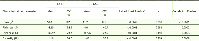
Paired t-tests showed clear differences between the ESB and GSB methods for each characterization parameter (Table 1). The most dramatic difference between methods was for density, which was more than 5 times higher in the ESB compared with the GSB. Although the difference in richness was not as large, the ESB still detected more than 30% more weed species than the GSB. Conversely, the differences between methods for diversity and evenness were smaller. For example, ESB diversity was only 9% higher than GSB diversity, while evenness was 10% higher in the GSB compared with the ESB. Although the variability of these two methods was similar (Table 1), the resulting characterization by all four parameters was different. The GSB is commonly used to compare treatment effects and to correlate soil seedbanks to emerged weed flora the following year (Forcella Reference Forcella1992; Cardina and Sparrow Reference Cardina and Sparrow1996). However, no conversion factor has been established between the GSB and ESB. Studies have found different weed compositions in the same seedbank because detection and overrepresentation of particular species might be favored depending on method (Abella et al. Reference Abella, Chiquoine and Vanier2013; Gonzalez and Ghermandi Reference Gonzalez and Ghermandi2012; Price et al. Reference Price, Wright, Gross and Whalley2010).
Comparison of estimation of weed community parameters for extractable (ESB) or germinable (GSB) seedbank methods using paired t-tests and Pearson’s correlation.

a Total number of individuals in 100 g soil.
b CV, coefficient of variation.
c Indicates the probability of significant differences between methods.
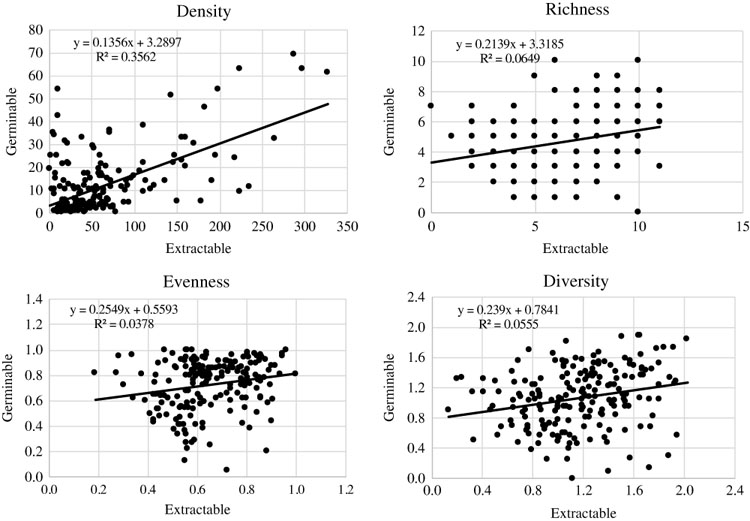
For all parameters studied, methods were weakly correlated, with coefficients ranging from 0.19 to 0.59 (Table 1). The correlation between ESB and GSB seed density was the only coefficient above 0.5, and thus seed density was the parameter with the largest differences in magnitude and highest variability. Regression analysis confirmed that all parameters had weak positive linear relationships between methods (Figure 1). The best-fit model for density described only 35% of the variation, but all other parameter models explained less than 7%, with the lowest under 4% (Figure 1). Due to the weak relationships, it would be difficult to create a conversion factor that could be reliably used to link both seedbank methods. While the methods have similar precision, these analyses demonstrate there is enough variability introduced by the method on species detection and density quantification that suggest they do not provide similar weed seedbank characterizations.
Relationship between extractable (ESB) and germinable (GSB) methods using paired samples for total weed density in 100 g soil; species richness (S); species evenness (J); Shannon-Weiner diversity (H′).

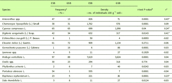
While ESB density was higher than GSB density overall (Table 1; Figure 1), this trend was not true for every species (Table 2). Only half of the species detected by both methods were found in higher quantity in the ESB (Table 2). Seedbank quantification tends to find different species compositions by different methods, commonly with several species unique to each method in addition to species common to both methods (Ball and Miller Reference Ball and Miller1989; Abella et al. Reference Abella, Chiquoine and Vanier2013). Paired t-tests confirmed that the total number of individuals of each species was different between methods, except for Ipomoea spp., Oxalis spp., and goosegrass [Eleusine indica (L.) Gaertn.] (Table 2).
Comparison of extractable (ESB) and germinable (GSB) seedbank methods by species composition.

a Relative frequency is the number of samples with at least one individual of the weed species divided by the total number of samples in the study.
b Indicates the probability of significant differences between methods for density.
c An asterisk (*) indicates that the correlation between methods was significant (α=0.05).
The density of most species did not correlate between the two methods, except for wild radish (Raphanus raphanistrum L.), Amaranthus spp., large crabgrass [Digitaria sanguinalis (L.) Scop.], and Cyperus spp., with r values of 0.23, 0.43, 0.41, and 0.24, respectively. Previous research indicated that the ESB often favored seeds based on size and density (Gross and Renner Reference Gross and Renner1989; Mesgaran et al. Reference Mesgaran, Mashhadi, Zand and Alizadeh2007; Tsuyuzaki Reference Tsuyuzaki1994), and the GSB favored seeds based on dormancy relief and germination requirements (Cardina and Sparrow Reference Cardina and Sparrow1996; Gonzalez and Ghermandi Reference Gonzalez and Ghermandi2012; Gross Reference Gross1990). While most comparison studies introduce a bias to the ESB method by using a floatation method, the present study uniquely exhumed the entire 200-g soil sample, even examining the sieved material for missed seeds. Granting the rigorous exhumation of the ESB, the fact that some species had greater detection in the GSB reinforces the idea that these methods cannot be used interchangeably.
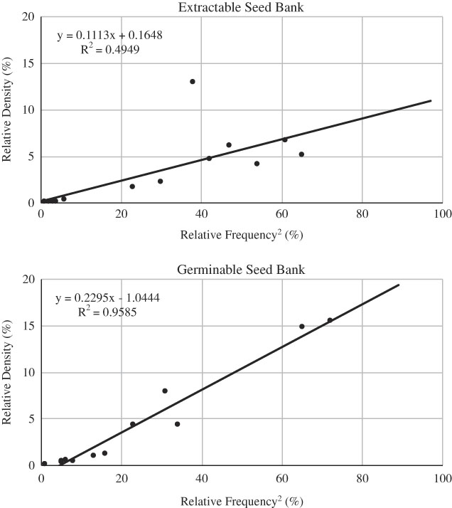
Species that occur more frequently may be predicted to have higher total densities, and this behavior is more likely to occur when the species is evenly distributed across the field or landscape. In the case of weed communities with rare species or species exhibiting highly aggregated distribution, it might be difficult to properly describe the richness and diversity of the community. In the present study, both methods had a positive relationship between the relative density of species and the relative frequency at which they occurred (Figure 2). Therefore, when enough samples are collected, both methods can generate data to successfully use techniques such as rarefaction to estimate weed species richness approximating the contribution of rare species (Koellner et al. Reference Koellner, Hersperger and Wohlgemuth2004; Rotches-Ribalta et al. Reference Rotches-Ribalta, Blanco-Moreno, Armengot, Chamorro and Sans2015). However, considering that the ESB exhibits higher weed species detection than the GSB, the former might be more useful for rarefaction analysis than the latter.
Relationship between relative species frequency and relative species density within extractable (ESB) and germinable (GBS) methods for seedbank characterization. Relative frequency was estimated as the number of samples in which a specific weed species was present based on the total number of samples in the study. Relative density was estimated as the total number of individuals of a species divided by the total individuals for each method.

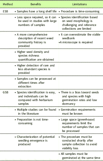
The results of the present study clearly showed that the ESB and GSB do not provide the same information to describe weed communities. In addition to having different quantification of certain species as reported by earlier studies, characterization of density, richness, evenness, and diversity differed between methods and lacked a consistent relationship. Nevertheless, it is interesting that although significant, the differences between methods for evenness and diversity were relatively small compared with density and richness. Therefore, estimating diversity and evenness might be a useful way to compare ESB and GSB studies, especially when rare species or species with low abundances within the community represent a minor proportion of the community or are ignored to emphasize predominant weed species. Furthermore, considering that both methods had similar precision (see coefficient of variation columns in Table 1), it is important to determine under what circumstances or for what objectives one might choose one method or the other (Table 3). The GSB is adequate when there is enough greenhouse space available for the number of samples and particularly important for studies that are comparing the effect of different treatments or conditions on the germinable seedbank. Also, this method requires less labor time per sample than the ESB. For example, in the present study, the GSB required an average of 18 min for sample preparation and analysis (including evaluation time), while the ESB required up to 73 min. Key aspects for improving the GSB method include providing opportunities to break dormancy by disturbing soil or cold stratification (Gross Reference Gross1990), deciding to use undisturbed cores or broken soil in trays (Cardina and Sparrow Reference Cardina and Sparrow1996), reducing space needed in the greenhouse by sieving soil to concentrate samples (Ter Heerdt et al. Reference Ter Heerdt, Verweij, Bekker and Bakker1996), or selecting the appropriate watering technique for the soil type (Espeland et al. Reference Espeland, Perkins and Leger2010). However, to characterize the seedbank while maximizing species detection and quantification, the ESB is still necessary, because it has the best chance of recovering rare species and seeds with long dormancy or specific germination requirements. Multiple efforts have been conducted to expedite seed extraction, including the use of flotation solvents (Buhler and Maxwell Reference Buhler and Maxwell1993; Tsuyuzaki Reference Tsuyuzaki1994), hydropneumatic elutriator (Gross and Renner Reference Gross and Renner1989), sieving, and cloth bag extraction (Mesgaran et al. Reference Mesgaran, Mashhadi, Zand and Alizadeh2007). Regardless of the technique used, when the extraction process is done carefully to minimize seed loss, the ESB is useful to process large number of samples, because the samples can be stored in a small area, and seed counts do not have to be done simultaneously for all samples. Researchers should be mindful of these benefits and limitations when considering the best method for study objectives. The present research presents information to help inform the selection of seedbank analysis methods to characterize weed communities for more efficient and reliable research results.
Benefits and limitations of extractable (ESB) and germinable (GSB) seedbank methods for weed community characterization.

Acknowledgments
No conflicts of interest have been declared. This research received no specific grant from any funding agency or the commercial or not-for-profit sectors. We want to thank Rocio van der Laat, Michael Dozier, Robert Murell, Sharon Howell, Timothy Ayankojo, and Ignacio Leon for technical support.