

Introduction
Recent research has shown that the amount of nitrogen (N) fertilizer applied in excess of crop uptake is an important determinant of N discharge from catchments in tropical Queensland, in which sugarcane production is a major land use (Thorburn and Wilkinson, Reference Thorburn and Wilkinson2013). Thus, increasing the efficiency of N use in cropping systems such as sugarcane is an important step in protecting the economic and ecological benefits provided by the Great Barrier Reef (Bell, Reference Bell2015). Importantly, an increase in N use efficiency (NUE) also offers opportunities to improve profitability, providing an incentive for practice change.
The key input criteria used in deriving N fertilizer management recommendations for sugarcane using the SIX EASY STEPS (6ES) system (Schroeder et al., Reference Schroeder, Wood, Moody, Bell and Garside2005, Reference Schroeder, Hurney, Wood, Moody and Allsopp2010; Schroeder, Reference Schroeder2009) are the yield potential (YP) of sugarcane and the N mineralization potential of the soil; the latter is estimated as a function of the soil organic matter content in the top 20 cm. Given the varied scale and availability of yield and soil information, 6ES is not prescriptive about the scale at which such information is brought to bear on the delivery of fertilizer recommendations. However, common practice is for 6ES to be implemented using a district yield potential (DYP) which is defined as the estimated highest average annual district yield (based on mill statistics collected since 1990) multiplied by 1.2 (Schroeder, Reference Schroeder2009). The DYP is multiplied by a factor to determine nitrogen required (1.4 kg N/t cane for the first 100 tonnes of cane and 1.0 kg N/t for additional tonnage above 100), and a discount is then applied based on soil organic carbon (%OC; for a 120 t/ha ratoon crop, the discount ranges from 10 kg N/ha when %OC is 0.41–0.8% up to 60 kg N/ha for %OC>2.4%).
The gradual adoption of Precision Agriculture (PA) technologies, such as yield monitors, has provided compelling evidence of significant variation in sugarcane yield at the within-field scale (Bramley and Quabba, Reference Bramley and Quabba2002; Johnson and Rickard, Reference Johnson and Richard2005; Bramley and Jensen, Reference Bramley and Jensen2013; Rodrigues et al., Reference Rodrigues, Magalhães, Franco, de Beauclair and Cerri2013; Bramley et al., 2017a). Likewise, the use of remote sensing as a yield prediction tool (Robson et al., Reference Robson, Abbott, Lamb and Bramley2012, Reference Robson, Rahman, Falzon, Verma, Ohansen, Robinson, Lakshmanan, Salter and Skocaj2016), suggests that yield may vary markedly within a given region. This variation raises questions as to the merits of using DYP as an input to 6ES from the perspective of NUE and the possible on- and off-site impacts of excessive N use (Bell, Reference Bell2015 and references therein).
This paper presents a spatial analysis of yield variation in the Herbert River district over seven seasons using mill records, together with analysis of yield variation at the field and farm scales using yield monitor data. Our aim is to move towards a more location-specific application of 6ES than is currently typically employed when based on DYP.
Materials and methods
We note at the outset that sugarcane is a grass which, when harvested, re-grows vegetatively as a ‘ratoon’ crop. A typical Australian sugarcane crop cycle would see cane planted as soon as is feasible after the wet season; that is, most likely around mid-late April. The resulting ‘plant crop’ is harvested approximately 15 months after planting, with the harvest season extending from early June to mid-late November. The ratoon crop is harvested approximately 12 months later, and the cycle continues, with each subsequent crop termed the ‘first ratoon’, ‘second ratoon’ and so forth. In a typical sugarcane rotation, the plant crop is followed by four ratoon crops, after which the fourth ratoon is ploughed out and the field either left fallow or planted to a break crop, typically a pulse, such as cowpea or soybean. This is then either harvested or ploughed in as a green manure before replanting sugarcane. Typically, a farm will be planted with a range of different sugarcane varieties. Note also that, for a range of reasons including the availability of planting material, previous crop performance and progress of the harvest, a typical sugarcane field or ‘block’ may comprise a number of ‘sub-blocks’ planted to cane of differing variety or age, both in terms of ratoon number (‘crop class’) and age since the last harvest. The collective result on any individual farm is an array of variety/crop class/crop age combinations.
For the district scale analysis reported here, sugar mill records from the 2009-2015 harvest seasons in the Herbert River district were used. For each of these seven harvest seasons, data were available on a sub-block basis covering yield of sugarcane (t/ha), variety and crop class (i.e. ratoon number). These data were geo-referenced to the centroid of sub-block boundaries pertinent to each record/year. Since 6ES makes no distinction between varieties, we assumed for this analysis that YP for all varieties in any given year was the same.
The district scale analysis followed the approach described by Bramley et al. (Reference Bramley, Ouzman and Gobbett2017b). In brief, mill data were filtered on the basis of crop class and data retained for plant crops and for first, second, third and fourth ratoon crops; data for crop classes older than fourth ratoon were discarded and data for standover cane (cane not harvested the previous year) were also discarded. Re-plant crops (i.e. when no fallow was used) were assumed to have the same YP as plant crops. For each crop class in each year, the retained data were normalized to a mean of zero and standard deviation of one, and any records that were not within +/−3 standard deviations of the mean were discarded.
For each crop class by year combination, maps of normalized yield were then interpolated onto a 100 m x 100 m raster grid derived from the boundary to the Herbert River cane growing area, using local block kriging in VESPER (Minasny et al., Reference Minasny, McBratney and Whelan2005) with a data cloud of 100 points (i.e. 100 sub-block records), exponential variograms and blocks of 500 m. In addition, for each year, the normalized crop class-based datasets were merged and a further map layer was interpolated summarizing annual yield variation for the district as a whole, independent of crop class. Typically, the support of crop class-based and ‘all crops’ maps was approximately 2,500 and 13,000 sub-block records respectively. Note that it was not possible to factor crop age since last harvest into this analysis.
For maps at the within-farm, -block and -sub-block scales, yield monitor data were used. These derived from an ongoing locally-implemented yield monitoring and harvester-tracking project being run in the Herbert River district (Lawrence DiBella, Herbert Cane Productivity Services Ltd – pers. comm.). The mapping of these data followed the protocol of Bramley and Jensen (Reference Bramley and Jensen2013), albeit using data that had been normalized (mean of zero, standard deviation of one) on a per harvest event basis, to remove artefacts due to crop age (time since harvest), crop class, varietal differences, mill consignment errors and yield monitor calibration. Following kriging, the maps were back-transformed to a t/ha basis using the mean yield calculated from mill records of sub-block tonnages and knowing the area harvested. The map data were then further adjusted to a first ratoon equivalent basis using a relationship describing ratoon yield decline (Bramley et al., Reference Bramley, Ouzman and Gobbett2017b).
Similarities in patterns of spatial variation in the mapped data between years were examined using k-means clustering in JMP (v.11.0.0, SAS Institute, Cary, NC, USA) with map display using the ArcGIS software suite (v10.4; ESRI, Redlands, CA, USA). In the case of block and farm scale data, the effects of missing yield data due to either the lack of crop (i.e. fallow) or yield monitoring equipment failure, were accommodated in the clustering using the method outlined by Bramley et al. (Reference Bramley, Jensen, Webster and Robson2017a) in which the mean value of normalized yield in years for which data are available is used as an estimate of normalized yield in the year of missing data, prior to back transformation using an appropriate local mean.
Results
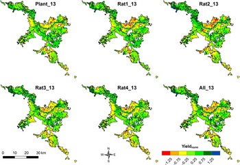
Irrespective of crop class, the patterns of variation in yield in any given year show marked spatial structure and follow a characteristic pattern when examined at district scale (Figure 1). Thus, when the normalized yield data for each crop class are pooled and a crop class-independent map generated (bottom right map in Figure 1), it has the same characteristic pattern of spatial variation in yield as is seen in maps interpolated on an individual crop class basis. This is in spite of the decline in mean yield from plant cane to fourth ratoon (Bramley et al., Reference Bramley, Ouzman and Gobbett2017b); mean yields of fourth ratoon over the study period were approximately 74% of those of plant cane in any given year.
Variation in the yield of sugarcane in the Herbert River district in 2013 for plant and first to fourth ratoon (Rat1-Rat 4) crops. Also shown (bottom right) is a map summarizing the variation across the combined crop classes. Note that the same legend applies to all maps and that the units of Yieldnorm are standard deviations; in 2013, the standard deviation in yield of first ratoon, for example, was 24.1 t/ha. Mean yields for each crop class (Plant-Rat4) were 86.6, 79.3, 73.6, 65.6 and 63.7 t/ha.

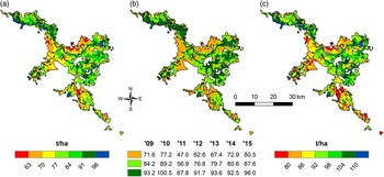
Very similar results to those obtained in 2013 (Figure 1) were obtained for each of the years 2009–2015 (not shown) such that when the crop class-independent maps (e.g. bottom right map in Figure 1) are compared across years, these also show the same characteristic pattern of within-district yield variation seen in Figure 1. Given the higher support of crop class-independent maps compared to those for a single class, they were used for conversion to a first ratoon equivalent basis knowing the district mean first ratoon yield in each year of the study. These were then used to map the mean yield of first ratoon equivalent crops over the 2009–2015 period (Figure 2a). They were also used for clustering using k-means, to identify zones of characteristic performance across seasons (Figure 2b) based on the reasonable assumption (Figure 1) that variation in yield of first ratoon characterized variation in any crop class. Since 6ES defines DYP on the basis of the estimated highest average annual district yield, it is of interest to examine variation in the maximum yield obtained at any location in addition to the mean. As Figure 2c clearly indicates, the pattern of variation in maximum yield is essentially the same as the pattern of variation in mean yield (Figure 2a); that is, characteristically low yielding areas also have the lowest maximum yield over the seven years of the study. In other words, the maps shown in Figures 1 and 2 provide a robust basis for consideration of spatial variation in YP (as opposed to actual yield) at regional scale, with Figure 2b offering one possible delineation of sub-regions for which different values of DYP might be assigned for the purposes of implementing 6ES.
Mean yield (a) of first ratoon sugarcane (2009–2015); (b) k-means clustering (3 cluster solution) of season specific maps; and (c) maximum yield (2009–2015) of first ratoon sugarcane in the Herbert River district.

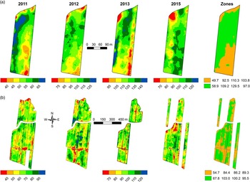
Unsurprisingly, yield maps displayed at either the whole farm, or block scale, also showed significant variation (Figure 3), and whilst the patterns of variation were less stable across seasons than has been observed previously (Bramley et al., Reference Bramley, Jensen, Webster and Robson2017a), clustering of the map data still enabled identification of potential management zones. In the case of the block scale (Figure 3a), the differences between zone means were of the order of 18% of the mean yield achieved in the lower yielding zone, except in 2015, whilst at the whole farm scale (Figure 3b), differences in zone means varied from approximately 7–24%. It is not known whether the smaller between-zone difference in 2015 might be attributable to any targeted remedial action, taken during replanting following the 2013 harvest, to improve performance in the lower yielding zones. However, the between-zone differences in mean yield are sufficient to warrant differential application of fertilizer N.
Variation in sugarcane yield 2011–2015 (no data were available in 2014) as measured using a yield monitor during harvest when mapped at either (a) the sub-block or (b) whole farm scale. In all cases, yields have been adjusted to a first ratoon equivalent based on sub-block mill records and the relative performance of different crop classes (Bramley et al., Reference Bramley, Ouzman and Gobbett2017b). Note that in (a) each map has its own legend; in (b) the legend shown for 2013 also applies to 2012 and 2015; and that the sub-block shown in (a) was second ratoon in 2011, third ratoon in 2012 and fourth ratoon in 2013 after which, it was replanted (no fallow) and so was first ratoon in 2015. Note also that the sub-block (a) is located to the central western side of the farm (b).

Discussion
The results suggest that there is a marked spatial variation in yield at regional scale in the Herbert River district, and that the patterns of this variation are stable across seasons and crop class. Importantly, the patterns of variation seen in all of the regional scale maps (Figure 1 and 2) are similar, a result which lends weight to the idea that there is no such thing as a single DYP that applies equally to all parts of the district. The results therefore provide a basis for moving away from the use of DYP as input to 6ES and, for those Herbert growers who have not yet adopted PA for the fine-tuning of fertilizer management at the within-block or -farm scales, a basis for a more location-specific application of 6ES. Since DYP, as used in 6ES, is based on the estimated highest average annual district yield, the map of variation in maximum yield obtained (Figure 2c) might provide a useful basis for location-specific estimates of YP.
For growers who have adopted PA, and/or have access to yield maps (e.g. Figure 3), such maps clearly provide a basis for targeted management of N at the within-block or within-farm scale. However, in the context of implementing 6ES at these scales, Figure 3 raises a potential problem. In the present analysis, we processed normalized yield data and following mapping, back-transformed it to a t/ha basis knowing the mean and coefficient of variation in yield; the data were then adjusted to a first ratoon equivalent using an expression describing yield decline as a function of ratoon number (Bramley et al., Reference Bramley, Ouzman and Gobbett2017b). Presumably due to the greater range of variation at the farm, compared to block scale, different values of the apparent zone mean yield are obtained when considered at the different scales. Thus, whilst the spatial structure in the data is retained when expressed at either block (Figure 3a) or farm scale (Figure 3b), different estimates of YP would be obtained if calculated as a function of the zone means at these different scales. Figure 3 also suggests that, in this example, inter-seasonal variation is greater than the effect of ratoon yield decline. It also suggests that, in contrast to the results of Bramley et al. (Reference Bramley, Jensen, Webster and Robson2017a), patterns of variation in yield at the within-block and -farm scale may vary sufficiently across seasons such that data spanning more than one crop cycle may be needed for delineation of management zones. Nonetheless, even if Figure 3 were used to estimate YP on the basis of the maximum yield obtained in each zone over the study period (c.f. Schroeder, Reference Schroeder2009; Schroeder et al., Reference Schroeder, Hurney, Wood, Moody and Allsopp2010), different N rates for each zone would be warranted.
Recently, in a study focused in a sugarcane field in the Burdekin region, Webster et al. (Reference Webster, Bramley and Jensen2016) used knowledge of yield variation at the within-block scale, coupled with measurement and modelling of the N budget, to demonstrate that under conventional uniform fertilizer management, areas of cane blocks that are low yielding are those which pose the greatest risk of N loss offsite. This is because they are the areas of lowest NUE. We therefore infer that, when fertilizer recommendations are made on the basis of DYP, characteristically low yielding areas within a cane growing district will be those where NUE is low and therefore where the risk of loss of N offsite is greatest. We therefore suggest that the kind of mill record-based analysis presented here could provide a useful basis for refining 6ES, or for that matter, any fertilizer recommendations based on a yield potential, and so improving N use efficiency. (Indeed, a similar approach could be used for other crops, for example grains, for which georeferenced records of deliveries to grain silos could be used.). For sugarcane grower adopters of PA, targeted N management within blocks will similarly lead to improved NUE and thus, a reduction in the risk of N loss to the Great Barrier Reef.
Conclusions
These results show that for the Herbert River district, there is no single value for DYP which can be uniformly applied to all Herbert cane fields. Accordingly, more location-specific estimates of YP, whether derived from mill records or yield monitors would provide a useful refinement to the implementation of 6ES and contribute to a reduced risk of off-site export of N from cane farms. Since the kind of data which underpin the regional scale analysis reported here are available in all Australian cane growing regions, similar analyses to those reported here are to be encouraged. Meanwhile, adoption of PA clearly has the potential to enable improved NUE and, as a consequence, improved environmental stewardship.
Acknowledgements
This work was jointly funded by CSIRO, Herbert Cane Productivity Services Ltd (HCPSL), Sugar Research Australia (SRA) and the Queensland Department of Environment and Heritage Protection through SRA project No. 2015_070. We are most grateful to Wilmar Sugar Pty Ltd for providing mill records and to HCPSL for providing yield monitor data. The support and assistance of Lawrence DiBella, Michael Sefton and Rod Nielson (HCPSL) and Raymond DeLai (Wilmar) in this work is gratefully acknowledged. Tony Webster (CSIRO) kindly commented on an earlier draft of the manuscript.