Multilevel Models

Multilevel models (also known as mixed models or hierarchical models) has been extensively covered in excellent manuals (e.g., Goldstein, Reference Goldstein2003; Hox, Reference Hox2010; Raudenbush & Bryk, Reference Raudenbush and Bryk2002). Data are characterized because sampling units are organized in a higher level of analysis. Thus, it is typically distinguished between Level–1 units (e.g., students, patients or workers) and Level–2 units (classrooms, hospitals or departments). Then, Level–1 units are clustered (or nested) in Level–2 units. It is expected that Level–1 units belonging to the same cluster correlates or show some dependency between them. Intraclass correlation index (ICC) measures the magnitude of dependency between Level–1 units and it is very important in multilevel models as an initial step (i.e., the null model that usually serves as an initial model) to test the importance of taking into account the two levels in the data. However, and more interesting, the various levels are not only a nuisance. Multilevel models permits the researchers to model simultaneously group and individual levels (i.e., combining them) in a single model. Multilevel models take into account different random effects simultaneously: There is not only one residual random variance to be explained, as occurs in conventional single-level regressions. Level–2 unit form is another random variance (i.e., intercept variance) to be modeled, and consequently, explained. And, if there are Level–1 effects that vary in Level–2 units, then random slopes may be relevant to be considered. This causes that several random sources of different levels are explained jointly that makes so attractive these models revealing contextual effects, cross-interaction effects and another desirable features that emerge from multilevel models.

We describe mathematically three models; two of them serve as examples to perform multiple imputation with all the R code explained (see Usage example section). We use the notation from Scott et al. (Reference Scott, Shrout and Weinberg2013).

The random intercept model with a Level–1 and Level–2 predictors are represented as:

(1) $$ {\mathrm{y}}_{\mathrm{ij}=}{\beta}_0+{\beta}_1\left({x}_{ij}\right)+{\beta}_2\left({w}_j\right)+{\mu}_{0j}+{\varepsilon}_{ij} $$

y_ij denotes the dependent variable for person i in the group j, $ {x}_{ij} $ is a Level–1 predictor; $ {w}_j $ denotes a Level–2 predictor. Fixed effects are denoted by $ {\beta}_0 $ (intercept model), $ {\beta}_1 $ is the Level–1 regression coefficient and $ {\beta}_2 $ is the Level–2 regression coefficient. Random effects are denoted by $ {\mu}_{0j} $ (Level–2 random intercepts) and $ {\varepsilon}_{ij} $ , Level–1 residuals. Random effects are aasassumed to be independent and follow normal distribution with mean zero and variances $ \tau 02 $ and $ \sigma e2 $ are assumed to be independent and follow normal distribution with mean zero and variances $ {\tau}_0^2 $ and $ {\sigma}_e^2 $ respectively.

The random slope model is represented as:

(2) $$ {y}_{ij=}{\beta}_0+{\beta}_1\left({x}_{ij}\right)+{\beta}_2\left({w}_j\right)+{\mu}_{0j}+{\mu}_{1j}\left({x}_{ij}\right)+{\varepsilon}_{ij} $$

Another Level–2 random effect emerges in this model: $ {\mu}_{1j} $ (Level–2 random slopes). Random Level–2 effects are assumed to be independent of Level–1 random effect. $ {\mu}_{0j} $ and $ {\mu}_{1j} $ are normally distributed with means = $ \left(\begin{array}{c}0\\ {}0\end{array}\right) $ , and variance-covariance, $ \Sigma =\left(\begin{array}{cc}{\tau}_0^2& {\tau}_{01}\\ {}{\tau}_{01}& {\tau}_1^2\end{array}\right) $ . Again, $ {\varepsilon}_{ij} $ are assumed to follow a normal distribution with mean 0 and constant variance $ {\sigma}_e^2 $ . Within the Bayesian framework the constant Level–1 variance assumption (homoscedasticity assumption) is not always necessary and different $ {\sigma}_e^2 $ can be accommodated (heteroscedasticity) (van Buuren, Reference Buuren and Hox2011). In fact, van Buuren (Reference Buuren and Hox2011) and Resche-Rigon and White (Reference Resche-Rigon and White2016) point out that multiple imputation methods that allow heteroscedasticity produces more reliable imputations. Other authors as Audigier et al. (Reference Audigier, White, Jolani, Debray, Quartagno, Carpenter, Buuren and Resche-Rigon2018) consider that homoscedasticity are only preferred in the presence of small sample size by groups. We will deal more extensively these issues later.

Finally, a model with a cross-level interaction will be expressed as:

(3) $$ {y}_{ij=}{\beta}_0+{\beta}_1\left({x}_{ij}\right)+{\beta}_2\left({w}_j\right)+{\beta}_3\left({w}_j\right)\left({x}_{ij}\right)+{\mu}_{0j}+{\mu}_{1j}\left({x}_{ij}\right)+{\varepsilon}_{ij} $$

Where the novelty is now the regression coefficient $ {\beta}_3 $ -which represent the joint effect of w and x on the dependent variable $ {y}_{ij} $ (usually, w is said to moderate the relation between Level–1 x variable and y dependent variable).

Mechanisms and Missing Data Patterns

Briefly, since these issues have been addressed extensively in numerous sources (e.g., Enders, Reference Enders2010; Schafer, Reference Schafer1997), it is important for the researcher to have some notion of the mechanisms and the patterns that generate missing data. Following Rubin classification system for missing data (1976), we have three general mechanisms generating missing data: Missing Completely At Random (MCAR), Missing At Random (MAR) y Missing Not At Random (MNAR). Suppose $ \mathbf{Y} $ is a data set partially observed ( $ {\mathbf{Y}}^{obs} $ ) and partially missing ( $ {\mathbf{Y}}^{miss} $ ) and $ \boldsymbol{\phi} $ represent the vector parameter of the missing data mechanism. Let be R the missing data indicator of $ \mathbf{Y} $ (1 if a score is observed and 0 if a score is missing). MCAR occurs when the probability of missing data is unrelated with the variable itself and unrelated to other observed variables. Formally, MCAR occurs when the distribution of missing data is $ P\left(\mathbf{R}|{\mathbf{Y}}^{obs},{\mathbf{Y}}^{miss},\boldsymbol{\phi} \right)=P\left(\mathbf{R}|\boldsymbol{\phi} \right) $ . Although MCAR is the most benign cause of missing data, this is unusual in correlational/observational studies and represents a very stringent assumption (except when the missing is planned by design). MAR is a more reasonable assumption and occurs when the distribution of missing data is $ P\left(\mathbf{R}|{\mathbf{Y}}^{obs},\boldsymbol{\phi} \right) $ , that is, R depends on the observed data and some parameter, $ \boldsymbol{\phi} $ , that relates $ {\mathbf{Y}}_{obs} $ with R. Finally, MNAR occurs when $ P\left(\mathbf{R}|{\mathbf{Y}}^{obs},{\mathbf{Y}}^{miss},\boldsymbol{\phi} \right) $ because R depends on (among other things) the unobserved data ( $ {\mathbf{Y}}^{miss} $ ).

Here it should be clarified that, while the researcher is interested in the parameters of his analysis/substantive model, $ \boldsymbol{\theta} $ (i.e., the model that guides research and answers a theoretical question), there are, as we see, the parameters responsible for the missing data, $ \boldsymbol{\phi} $ , usually considered a nuisance parameters. Rubin’s (Reference Rubin1976) work established the conditions where, $ \boldsymbol{\phi} $ do not interfere with $ \boldsymbol{\theta} $ (which is what would happen if a researcher was fortunate enough to have all the observed data). Under MCAR or MAR missing mechanisms, Rubin demonstrated that treatment strategies for missing values by Full Information Maximum Likelihood and by Multiple Imputation do not need to consider (to estimate) $ \boldsymbol{\phi} $ to consistently and efficiently estimate $ \boldsymbol{\theta} $ (i.e., the substantive parameters). This is what is known in the literature as ignorable missingness.

The pattern of missing data refers to the configuration of missing data. This is clearly nowadays less important than mechanisms but, initially, when the first algorithms were developed to treat missing data, the configuration was important (not now, as the algorithm work well regardless of the patterns). For example, a very distinguishable pattern (called, monotone pattern) occurs in clinical longitudinal studies due to attrition phenomena: a patient who leaves the study no longer has values observed in the following waves. However, in multilevel analysis it is still important to consider whether the missing data is due to a systematic or sporadic pattern (in fact, our proposed guide takes into account this patters, see Table 3). When some variables are fully unobserved in some clusters (for example, all the students in some classrooms do not answer to some relevant performance measures), this is a systematically missing data pattern (Audigier et al., Reference Audigier, White, Jolani, Debray, Quartagno, Carpenter, Buuren and Resche-Rigon2018). As opposed, sporadically missing data patters are specific to each individual observation (does not affect the whole cluster to which the individual belongs).

Table 1.

Methods to Conduct Univariate Multilevel Imputation Via FCS

TABLE 2

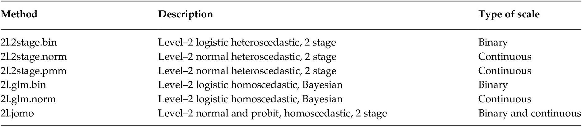
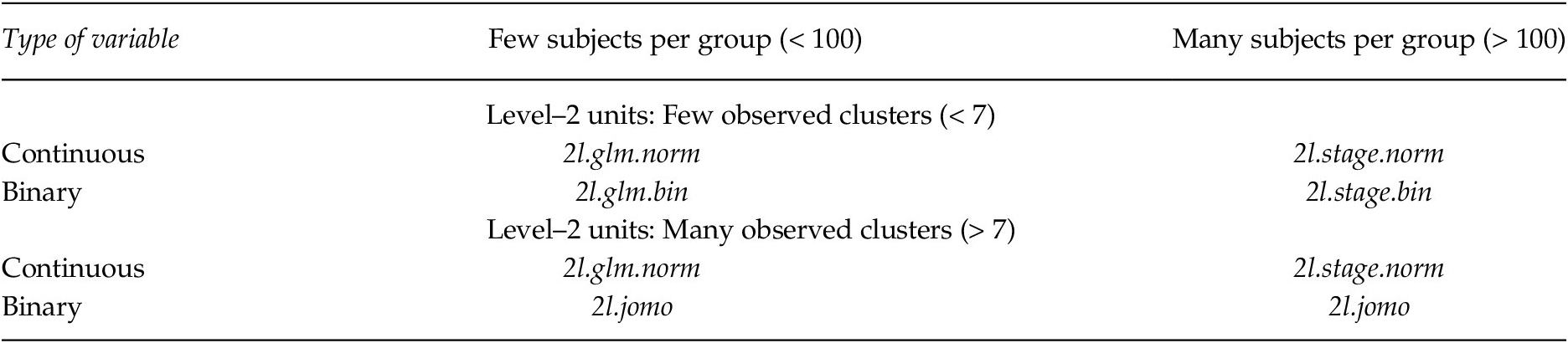
FCS Imputation Methods in R Mice Package depending on the Sample Size

TABLE 3.

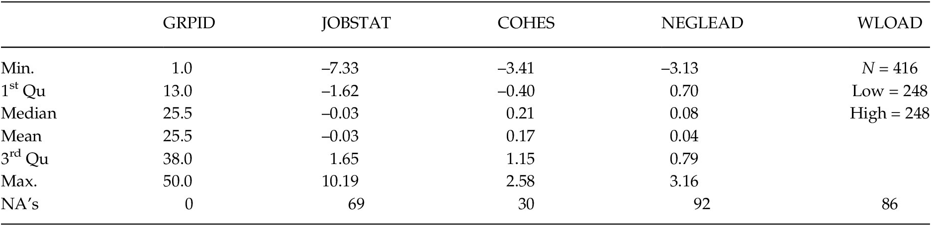
Descriptive Statistics of Leadership Data Set

Multiple Imputation

Traditionally, when a researcher have to deal with the problem of missing data, a case deletion strategy (also known as listwise deletion or an omitted strategy) has been followed (this is the option that is set by default in many commercial statistical packages). This strategy consist of simply ignoring those cases which missing data. Consequently, case deletion is computationally simple as the algorithms work with complete matrices. The counterpart is that it relies on very strong assumptions. Case deletion only is appropriate (unbiased) when MCAR is the missing data mechanism, often, as has been pointed out, an unrealistic assumption. We discard in the following case deletion strategy, as the modern lines to handle missing has been extensively developed for decades (Little & Rubin, Reference Little and Rubin2002; Schafer, Reference Schafer1997). They are usually referred to as Full Information Maximum Likelihood (hereafter referred to as FIML) and Multiple Imputation (hereafter referred to as MI) methods, appropriate when missing data is MCAR or MAR.

Enders (Reference Enders2017) or Grund et al. (Reference Grund, Lüdtke and Robitzsch2018) has pointed out that FIML is a good strategy to manage missing data in multilevel models when missing values are only circumscribed to the dependent variable. However, they currently claim that MI is the best general method to handle missing data in multilevel models. It is because MI is better suited to a variety of scenarios. Accordingly, in this work, we will not recommend FIML to applied researchers. Instead, as the state of the art focuses on MI methods within multilevel models, we will consider this method bellow.

As mentioned, MI is more flexible since it deals with missing data in Level–1 and Level–2 predictors variables (and not only in the dependent variable). MI is well suited for a great variety of multilevel models: It works appropriately in random intercept models, random slope models, models that estimate contextual effects or models with cross-level interactions. MI has proven to work well with incomplete categorical covariates, combination of continuous and categorical predictors or models that include auxiliary variables in order to better estimate missing values.

MI is characterized by three phases: The imputation phase, the analysis phase and the pooling phase. In the imputation phase MI generate multiple copies of the original (and incomplete) data set, each of which containing different estimates of the missing values. This phase is the most technical and important one, so we devote the next paragraphs to this phase. The analysis phase is simple, as it estimates the analysis or substantive model in each of the filled-in copies generated in the previous phase. In fact, the copies can be imputed with different software than that used for the analysis phase. In the pooling phase, the parameters estimated in each data set are combined into a single set of results. The estimates and standard errors are then pooled according to Rubin's rules (Reference Rubin1987).

Paying our attention to the imputation phase, to be clear for the reader, a distinction is made between the analysis model and the imputation model. The analysis model is the model on which the researcher focuses his or her theoretical interest and motivates the research. The imputation model is the one intended to generate copies of the database that will later allow the analysis model to be correctly estimated (i.e., to make valid inference and valid estimates). It is crucial that there is compatibility (also known as congeniality) between the imputation model and the analysis model (e.g., Enders, Hayes, et al., Reference Enders, Hayes and Du2018). The general rule is that the imputation model must at least consider all the effects estimated in the analysis model. When the imputation model omits important effects, this produces uncongenial models. For example, if an interaction effect is present in the analysis model and is not included in the imputation model, subsequent analyses can attenuate the interaction effect (Enders, Reference Enders2010).

In the imputation phase, whose aim is to create several copies from the imputation model, there are two clearly separate steps: The posterior-step and the imputation-step (for details see Enders, Reference Enders2010, pp. 190–194; Enders, Keller, et al., Reference Enders, Keller and Levy2018). This iterative two-step algorithm approach samples parameter values from the imputation model and uses the parameters to define a distribution of imputed values. In the posterior-step a Bayesian analysis describe the posterior distribution of $ {\boldsymbol{\theta}}^{\boldsymbol{I}} $ which depends on $ {\mathbf{Y}}^{obs} $ , that is, P( $ {\boldsymbol{\theta}}^{\boldsymbol{I}}\left|{\mathbf{Y}}^{obs}\right) $ where $ {\mathbf{Y}}^{obs} $ represents the observed information and $ {\boldsymbol{\theta}}^{\boldsymbol{I}} $ is a vector of parameters of the imputation model (superscript I is included to differentiate the parameters of the imputation model from those of the analysis model). MI relies heavily on Bayesian methodology, but exists alternatives to draw parameters in the posterior-step as to draw them via REML, two-stage estimator, etc. (e.g., for other strategies see Audigier et al., Reference Audigier, White, Jolani, Debray, Quartagno, Carpenter, Buuren and Resche-Rigon2018). Here we base our explanation in the commonly Bayesian strategy. The posterior-step estimation usually is based in a Gibbs sampler algorithm (which pertain to a more widely and general estimation method known as Markov Chain Monte Carlo or MCMC) which has had exponential growth during the last years (Gelman & Hill, Reference Gelman and Hill2007). In the imputation step, MI replaces missing values based on the observed data and the statistical model (the imputation model). The replacements (also known plausible values) are generated by drawing from the posterior predictive distribution of the missing data, given the observed data and the parameters of the imputation model (Grund et al., Reference Grund, Lüdtke and Robitzsch2018). More formally, the plausible imputed values come from the imputation model, P( $ {\mathbf{Y}}^{miss}\left|{\mathbf{Y}}^{obs},{\boldsymbol{\theta}}^{\boldsymbol{I}}\right) $ , where $ {\mathbf{Y}}^{miss} $ represents the missing information.

Imputation Phase: JM and FCS

The imputation phase differentiates between two general strategies or frameworks to drawing plausible values from the posterior predictive distribution of the missing data: Joint modeling (JM) and fully conditional specification (FCS) (see, for example, Enders, et al., Reference Enders, Mistler and Keller2016, p. 4; Enders, Hayes, et al., Reference Enders, Hayes and Du2018, pp. 697–701; Grund, et al., Reference Grund, Lüdtke and Robitzsch2018, pp. 114–115; van Buuren, Reference Buuren2018). The reader may find this section somewhat more technical. It is not necessary to follow the guidelines proposed below, but it gives an idea of the basic notions that differentiate one strategy from another. Both strategies have different versions and just to illustrate their differences, we present JM and FCS in the random slope model, where both the outcome and the predictor variables have missing values. Suppose the analysis model is (this is the model introduced in Equation 2 without the Level–2 predictor to make easier the explanation):

(4) $$ {y}_{ij=}{\beta}_0+{\beta}_1\left({x}_{ij}\right)+{\mu}_{0j}+{\mu}_{1j}\left({x}_{ij}\right)+{\varepsilon}_{ij} $$

This is a random slope model (i.e., the effect that predictor x has on y is not the same in all clusters), where $ {y}_{ij} $ is the score of the outcome variable for the subject i in the cluster j, $ {x}_{ij} $ is the Level–1 predictor variable. $ {\beta}_0 $ and $ {\beta}_1 $ are the fixed effects (intercepts and slope coefficients, respectively), $ {\mu}_{j0} $ is the Level–2 random intercept, $ {\mu}_{1j} $ is the Level–2 random slope and $ {\varepsilon}_{ij} $ is the Level–1 residual.

Joint Modeling: The JM imputation model is a multivariate regression modelFootnote ¹:

(5) $$ {y}_{ij}={\gamma}_{(y)}+{\upsilon}_{j(y)}+{e}_{ij(y)} $$

$ {x}_{ij}={\gamma}_{(x)}+{\upsilon}_{j(x)}+{e}_{ij(x)} $

where $ {\gamma}_{(y)} $ and $ {\gamma}_{(x)} $ are the fixed effects (intercepts), $ {\upsilon}_{j(y)} $ and $ {\upsilon}_{j(x)} $ Level–2 random intercepts, $ {e}_{ij(y)} $ and $ {e}_{ij(x)} $ Level–1 residuals, both normally distributed: $ \left(\begin{array}{c}{\upsilon}_{j(y)}\\ {}{\upsilon}_{j(x)}\end{array}\right)\sim N\left(0,{\Sigma}_{\upsilon}\right) $ , $ \left(\begin{array}{c}{e}_{ij(y)}\\ {}{e}_{ij(x)}\end{array}\right)\sim N\left(0,{\Sigma}_{ej}\right) $ . In addition, $ {\Sigma}_{\upsilon } $ and $ {\Sigma}_{ej} $ are distributed under the inverse Wishart distributionFootnote ². In the posterior step, Bayesian estimation via MCMC algorithms (e.g., Gibbs sampler, see Schafer & Yucel, Reference Schafer and Yucel2002, for details) draws plausible estimates from the posterior distribution of the imputation model parameters (details can be consulted, for example, in Enders, Hayes, et al., Reference Enders, Hayes and Du2018). Then, once the parameters has been drawn, the imputation-step takes place. JM draws missing values at once from a join probability distribution (usually multivariate normal distribution), where the estimated parameters in the posterior-step are used to replace missing values from a multivariate normal distribution (the t superscript reflects iteration t):

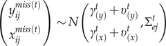(6) $$ \left(\begin{array}{c}{y}_{ij}^{miss(t)}\\ {}{x}_{ij}^{miss(t)}\end{array}\right)\sim N\left(\begin{array}{c}{\gamma}_{(y)}^t+{\upsilon}_{(y)}^t\\ {}{\gamma}_{(x)}^t+{\upsilon}_{(x)}^t\end{array},{\Sigma}_{ej}^t\right) $$

Fully Conditional Specification: Unlike JM, FCS draws missing value from univariate distribution conditioned to other model variables (see, for example, Carpenter & Kenward, Reference Carpenter and Kenward2013; Hughes et al., Reference Hughes, White, Seaman, Carpenter, Tilling and Sterne2014). Now, imputations is variable-by-variable, where it is used a series of univariate regression models with an incomplete variable regressed on complete and previously imputed variables. In each imputation step, the missing values for a particular variable are replaced from a conditioned distribution to all other variables, including variables that have been filled in the previous step. In FCS the researcher has to choose the imputation method for each incomplete variable of the model (e.g., linear regression if the outcome variable is continuous, logistic regression if the outcome variable is binary, etc.). Following the previous analysis model, for FCS the imputation models for y and x are:

(7) $$ {y}_{ij}={\gamma}_{0(y)}+{\gamma}_{1(y)}{x}_{ij}+{\gamma}_{2(y)}{\overline{x}}_j+{\upsilon}_{0(y)}+{\upsilon}_{1(y)}{x}_{ij}+{e}_{ij(y)} $$

where, $ {\upsilon}_{0(y)} $ and $ {\upsilon}_{1(y)} $ follows a bivariate normal distribution, $ \left(\begin{array}{c}{\upsilon}_{0(y)}\\ {}{\upsilon}_{1(y)}\end{array}\right)\sim N\left(0,{\Sigma}_{\upsilon (y)}\right) $ , and $ {e}_{ij(y)} $ is also normally distributed, $ {e}_{ij(y)} $ $ \sim N\left(0,{\sigma}_{e(y)}^2\right) $ .

(8) $$ {x}_{ij}={\gamma}_{0(x)}+{\gamma}_{1(x)}{y}_{ij}+{\gamma}_{2(x)}{\overline{y}}_j+{\upsilon}_{0(x)}+{\upsilon}_{1(x)}{y}_{ij}+{e}_{ij(x)} $$

where, $ \left(\begin{array}{c}{\upsilon}_{0(x)}\\ {}{\upsilon}_{1(x)}\end{array}\right)\sim N\left(0,{\Sigma}_{\upsilon (x)}\right) $ , and $ {e}_{ij(x)} $ $ \sim N\left(0,{\sigma}_{e(x)}^2\right) $ .

Again, Bayesian estimation is conducted with MCMC algorithms and estimates parameters are sampled from the posterior distribution. After that, imputation-step takes place and missing values are replaced based on previously estimated parameter (note that the parameters contain the superscript t, while the imputed values depend on the previous t – 1 iteration):

(9) $$ {y}_{ij}^{miss(t)}\sim N\left({\gamma}_{0(y)}^{(t)}+{\gamma}_{1(y)}^{(t)}{x}_{ij}^{\left(t-1\right)}+{\gamma}_{2(y)}^{(t)}{\overline{x}}_j^{\left(t-1\right)}+{\upsilon}_{0j(y)}^t+{\upsilon}_{1j(y)}^{(t)}{x}_{ij}^{\left(t-1\right)},{\sigma}_{e(y)}^2\right) $$

(10) $$ {x}_{ij}^{miss(t)}\sim N\left({\gamma}_{0(x)}^{(t)}+{\gamma}_{1(x)}^{(t)}{y}_{ij}^{(t)}+{\gamma}_{2(x)}^{(t)}{\overline{y}}_j^{(t)}+{\upsilon}_{0j(x)}^t+{\upsilon}_{1j(x)}^{(t)}{y}_{ij}^{(t)},{\sigma}_{e(x)}^2\right) $$

Therefore, both strategies (JM and FCS), although addressing imputation differently, both go through by means of an iteratively algorithm, usually a Gibbs sampler algorithm, the two described steps (i.e., posterior-step and imputation-step). In the posterior-step values of $ {\boldsymbol{\theta}}^{\boldsymbol{I}} $ are sampled from the posterior distribution P( $ {\boldsymbol{\theta}}^{\boldsymbol{I}}\left|{\mathbf{Y}}^{obs}\right) $ . Then, in the imputation-step, missing values are replaced from the predictive distribution P( $ {\mathbf{Y}}^{miss}\left|{\mathbf{Y}}^{obs},{\boldsymbol{\theta}}^{\boldsymbol{I}}\right) $ . 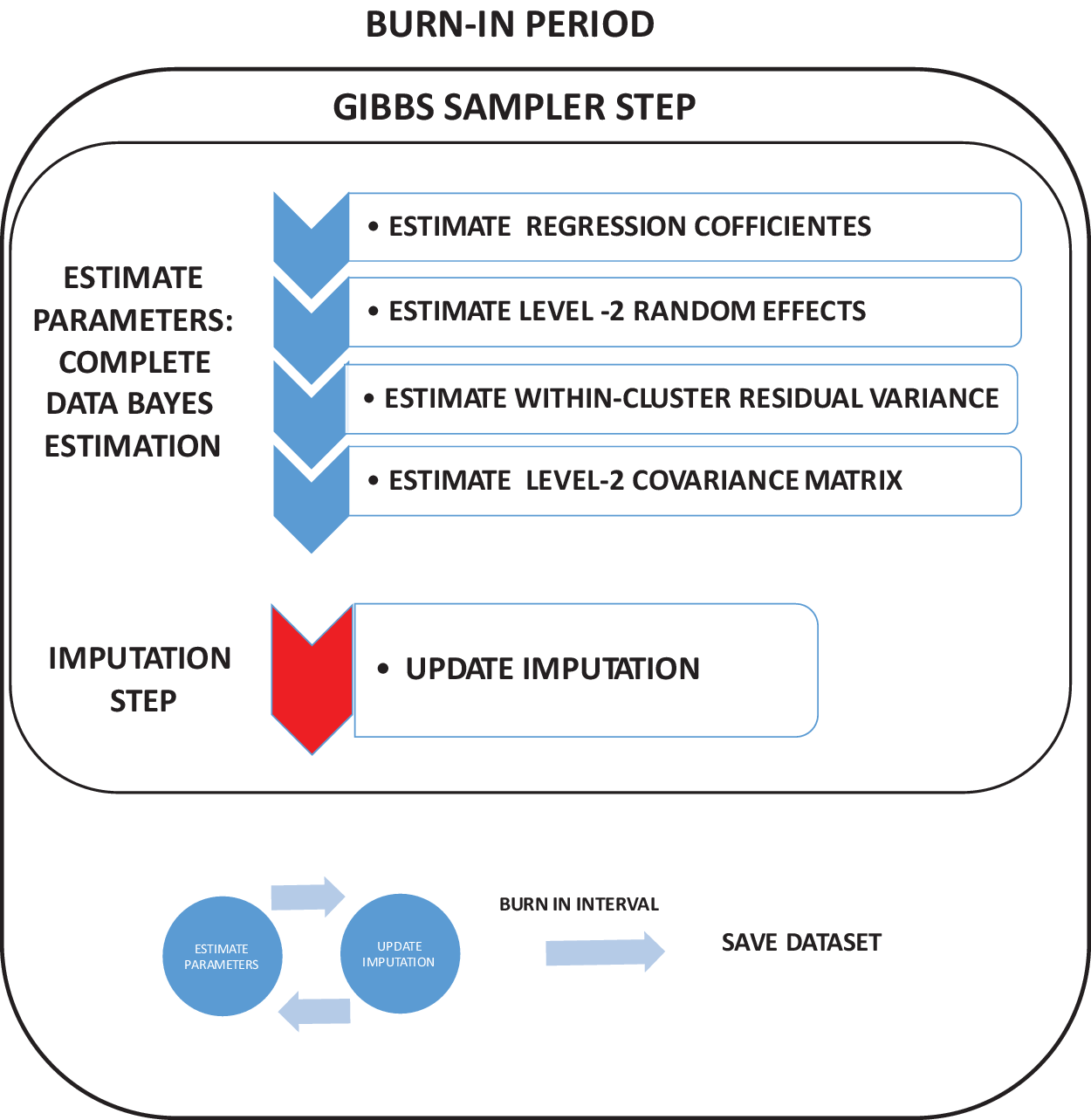Figure 1 schemes the aforementioned steps. Note that the figure details the parameters that are estimated in a multilevel model (fixed effects, random effects and random covariances), shows the imputation-step and ends up illustrating a filled-in data set after a burn-in period. This two-step algorithm works iteratively. A burn-in period needs to be established. That is, when the data is imputed it is necessary an initial burn-in period before datasets are generated to ensure the parameters distribution are stabilized (i.e., to ensure a stationary posterior distribution is reached). After the first dataset is generated the researcher must specify some number of cycles between imputation and imputation (i.e., a number of between-imputation iterations, see Enders, Reference Enders2010, p. 211). The researcher must pay especially attention to convergence criteria when conducting MI imputation methods (Enders, Reference Enders2010).

Figure 1.

Scheme of the Gibbs Sampler Algorithm to Impute Values in Multilevel Models

Note. General scheme of the Gibbs sampler algorithms. In the Bayesian approach first the $ \boldsymbol{\theta} $ is estimated in four steps: First is the fixed regression coefficients are estimated, followed by the Level-2 random effects (usually intercepts and slope for the Level-2 units). Then Level-1 variance is estimated. Finally, the Level-2 covariance (e.g., intercept and slope variance and intercept-slope covariance) is estimated. After that, this is conducted the imputation step where missing data is filled.

Convergence Criteria in JM and in FCS and Auxiliary Variables

Convergence criteria: As we already know, in the imputation phase of the JM models, a predetermined number of datasets are generated (say, m datasets). These datasets are not imputed consecutively because the MCMC would causes autocorrelation between generated (imputed) datasets. Thus, the algorithm (e.g., Gibbs sampler) performs a series of iterations without saving data ensuring the imputation parameters of the model have converged into stationary distributions (e.g., 5,000 iterations can be adequate). This is the way to generate independent imputations and this is the reason because the convergence criteria is not such easy as it is in other estimation methods (e.g., ML methods). The multiple imputation methods we are considering in this paper, e.g., those implemented in jomoImpute( ) function of the R package mitml as we will see later, takes as an argument the number of iterations until burn-in, n.burn argument in jomoImpute( ) function, and the number of iteration between two consecutive imputed data sets, n.iter argument in jomoImpute( ) function. For example, as a default argument these functions generate 5,000 iterations and a separation of 100 iteration between imputed datasets. In the Joint Modeling Example 1, we will see how to parameterize both arguments. A common criterion for examining convergence is to use what is known as potential scale reduction which it is recommended to be below 1.050 (Enders, Reference Enders2010; Gelman & Rubin, Reference Gelman and Rubin1992). This numeric criterion is included in the R package mitml package. This package also offers the user a series of diagnostic graphs (a description of these graphs can be found in Grund et al., Reference Grund, Robitzsch and Lüdtke2019).

In the burn-in phase of the FCS models, the necessary amount of major iterations to achieve convergence is much smaller than in the case of JM. The key why FCS algorithms achieve such rapid convergence is that they create univariate regression imputation models that are independent. In the R package we will recommend for FCS strategy, mice package, convergence can be reached in as few as 10 or 20 iterations (van Buuren & Groothuis-Oudshoorn, Reference Buuren and Groothuis-Oudshoorn2011). The number of iterations for burn-in is also an argument of the imputation function mice ( ) (the argument is maxit which has 5 default iterations). The complete procedure produces an imputed database.

As with JM, with FCS the researcher must ensure that the algorithm has converged and the imputed data are independent. What is frequently done is to interpret the diagnostic graphs (for example, see in mice manual from van Buuren & Groothuis-Oudshoorn, Reference Buuren and Groothuis-Oudshoorn2011, pp. 38–39 graphs for convergence and non-convergence estimation parameters). We will visit these diagnostic graphs in the Examples 1 and 2 (and we will explain them there).

Auxiliary variables: In general, within MI has been extensively recommended what is called as an inclusive strategy (see Collins et al., Reference Collins, Schafer and Kam2001; Graham, Reference Graham2003). This means that in the imputation model it is recommended to include all the variables that can account for missing data (including second-order effects such as interactions, polynomial terms, etc., if these help in the imputation). The more predictors in the imputation model, the more plausible the data loss mechanisms are MAR (as opposed to MNAR, see van Buuren & Groothuis-Oudshoorn, Reference Buuren and Groothuis-Oudshoorn2011, p. 22). Despite this recommendation, some caution should be taken so as not to generate an unwieldy imputation model. For example, in practice, models with a maximum of 15–25 variables in the imputation model usually work well and more variables can lead to problems (e.g., multicollinearity, convergence problems, etc.) (van Buuren & Groothuis-Oudshoorn, Reference Buuren and Groothuis-Oudshoorn2011, p. 15). It is recommended that the imputation model contains all the variables of the analysis model (if not, the uncongeniality problem may arise causing bias estimates). In addition, imputation model should include all variables related with nonresponse (e.g., categorical variables related with the probability of nonresponse, continuous variables in which differ respond and nonrespond groups, etc.). Therefore, the researcher should make a careful examination of his/her data before specifying an imputation model, so that he/she can collect all the auxiliary variables that are of interest. Finally, it should be noted that including auxiliary variables which, in turn, have high ratios of missing data, can causes estimation problems and should be avoided.

Software

The methods (and recommended libraries) that we will use for this guide are the most relevant and current from the author's point of view.

Joint Modeling methods. Which package: For joint modeling (JM) we recommend to use mitml package with jomo method (Quartagno & Carpenter, Reference Quartagno and Carpenter2020). jomo method is included in mitml package as jomoImpute function. Why: mitml is recommended for its versatility (Grund et al., Reference Grund, Robitzsch and Lüdtke2019). This package incorporates convergence diagnosis statistics, analysis and pooling phase facilities, visualizations tools, and include methods (as jomo) with the capacity to handle categorical (not only continuous) variables, heteroscedasticity within-cluster variance and manage systematic and sporadic missing data. Studies: The recommendation is supported by extensive simulation work carried out by Enders, Hayes, et al. (Reference Enders, Hayes and Du2018), Grund et al. (Reference Grund, Lüdtke and Robitzsch2016, Reference Grund, Lüdtke and Robitzsch2018), Audigier et al. (Reference Audigier, White, Jolani, Debray, Quartagno, Carpenter, Buuren and Resche-Rigon2018) or van Buuren (Reference Buuren2018). Note the reader that there are other JM methods that are well tested as pan (Schafer & Yucel, Reference Schafer and Yucel2002; Yucel, Reference Yucel2008) realcome (Carpenter & Kenward, Reference Carpenter and Kenward2013) and jm-mplus (Asparouhov & Muthén, Reference Asparouhov and Muthén2010), but they are subsumed in jomo method. When: we recommend using jomo method in multilevel random intercept and contextual models with missing Level–1 and missing Level–2 predictor variables (continuous and categorical). We choose these models because jomo has shown very good properties in the previous cited works dealing with random intercept models (unbiased estimates, good coverage for confidence intervals, efficient standard errors, and so on). Although some works show that jomo is a good enough method (but not perfect) for models with random slopes or cross-level interaction (Enders, Hayes, et al., Reference Enders, Hayes and Du2018), they tend to present some problems when estimate random slope variance or fixed cross-level coefficient, especially when the number of clusters are small.

Fully Conditional Specification methods. Which package: Among FCS strategy, we will use the mice package (van Buuren & Groothuis-Oudshoorn, Reference Buuren and Groothuis-Oudshoorn2011; van Buuren et al., Reference Buuren, Groothuis-Oudshoorn, Robitzsch, Vink, Doove and Jolani2015) and its micemd plugging (Audigier & Resche-Rigon, Reference Audigier and Resche-Rigon2018). This package contains several proven methods; some of them are shown in Example 2: 2l.gml (General Linear Model, see Jolani et al., Reference Jolani, Debray, Koffijberg, Buuren and Moons2015) and 2l.2stage (Resche-Rigon & White, Reference Resche-Rigon and White2016). Why: Mice library has an extensive reputation over more than one decade and incorporates visual methods for convergence diagnosis, the possibility of using univariate imputation models that accommodate variables with different metrics (binary, categorical, continuous, counts) and, among other things, facilities for the analysis and pooling phases. Studies: 2l.gml, 2l.jomo and 2l.2stage have shown good properties in simulation works: Audigier et al. (Reference Audigier, White, Jolani, Debray, Quartagno, Carpenter, Buuren and Resche-Rigon2018), Kunkel and Kaizar (Reference Kunkel and Kaizar2017), Resche-Rigon and White (Reference Resche-Rigon and White2016) and van Buuren (Reference Buuren2018). As occurs with JM, there are other FCS methods such as 2l.norn (van Buuren, Reference Buuren and Hox2011) or, for example, FCS-Blimp a very promising method that still need to be tested (Keller & Enders, Reference Keller and Enders2019). For FCS we will use the methods in Table 1. The difference between 2l.2stage and 2l.glm methods will be in the average sample size per cluster (see later Table 2). When the sample size of the clusters is large enough 2l.2stage are recommended and when sample size is small, it is preferable to use 2l.glm (Audigier et al., Reference Audigier, White, Jolani, Debray, Quartagno, Carpenter, Buuren and Resche-Rigon2018). 2l.jomo is reserved for when missing data occurs in a binary variable. When: We recommend using FCS methods in models with random slopes and models with cross-level interaction, especially when missing data affects to predictors involved in the random slope or cross-interactions (e.g., Ender et al., Reference Enders, Mistler and Keller2016; Enders, Keller, et al., Reference Enders, Keller and Levy2018 or Grund et al., Reference Grund, Lüdtke and Robitzsch2018) .

Guideline

We must consider the following steps when a researcher wants to do MI within multilevel models. Of course, the guideline is for multilevel structure data and, simultaneously, presence of missing data. The steps in the guide are concreted in the following section with two examples.

First: Should the researcher use an MI strategy or can he use simpler procedures? The researcher must consider whether it is worthy to analyze her data with MI for multilevel data since the procedure involves complexities that can be avoided. Before analyzing missing data with MI, Grund et al. (Reference Grund, Lüdtke and Robitzsch2016) and Enders et al. (Reference Enders, Hayes and Du2018) studies show that multilevel models can be analyzed using FIML if the outcome variable is the only variable with missing data. This scenario is not, at all, unusual in experimental designs, where the only variable with missing data is the dependent variable (the independent variables usually refer to manipulated experimental conditions in which there is rarely any missing data). This is the default method specified in commercial software as SPSS or R’s lmer library. When this is the case, FIML is an unbiased and efficient method of estimating parameters of the analysis model (naturally, assuming that missing data is due to MCAR or MAR mechanisms).

Therefore, the most complex decisions have to be considered when missing data affects covariates. The simplest method is listwise deletion and this is the method used in commercial software (e.g., again, SPSS) or lmer library. Grund et al. (Reference Grund, Lüdtke and Robitzsch2016, p. 648) affirm that listwise deletion “should be avoided when covariate data are missing, unless data are strictly MCAR”. However, if the sample is large enough and MCAR can be assumed (typically in designs where missing is planned) listwise deletion is an alternative because of its simplicity (the researcher does not really have to make any explicit decision concerning the missing data). Note that experts warn against the use of listwise deletion especially if the missing values affect Level–2 covariates (van Buuren, Reference Buuren2018).

As we already know, multilevel models are necessary because the grouped data violates the assumption of independence. The Intraclass Correlation Coefficient (ICC) expresses the amount of dependence. As a rule of thumb, when the ICC is less than .10 and the proportion of missing data is less than 5%, single-level imputation can be used (i.e., standard routines can be applied without worrying about the multi-level structure). In this scenario, a conventional FCS can be used or fixed effects through dummy variables in another possibility (see Drechsler, Reference Drechsler2015). In other cases (e.g., ICC above .10, more than 5% of missing data or when the researcher are interested in the random effects of the model) we will always use multiple imputation models (Grund et al., Reference Grund, Lüdtke and Robitzsch2018; van Buuren, Reference Buuren2018).

Second. Mechanisms. As we know, the assumption of ignorability implies MCAR or MAR mechanisms (Rubin, Reference Rubin1976). The general rule in research is that, unless the non-response is followed up (i.e., explicitly tracking the causes of non-response), it is not possible to test the mechanism underlying the missing values (see Raykov, Reference Raykov2011). Many times the mechanisms behind missing data are multiple (e.g., a mixture of MCAR, MAR and MNAR, together). For minimize the negative impact of MNAR causes, the researcher can use as much auxiliary variables as can (van Buuren & Groothuis-Oudshoorn, Reference Buuren and Groothuis-Oudshoorn2011, p. 22). This approximate an MNAR mechanism into an MAR mechanism (often, using auxiliary variables account for the missing data causes). Although mice R package can handle MNAR multiple imputation (see van Buuren, Reference Buuren and Hox2011, section 6.2) we do not recommend it.

Third. Distinguish between the imputation model and the analysis model. We must specify an appropriate imputation model. For this, the researcher must take into account that the analysis model and imputation models must be congenial. Although this is a technical issue, this means that the analysis model is nested or subsumed in the imputation model (remember that imputation model has to be more general). Therefore, the variables of the analysis model, the estimated parameters and all the relationships (for example, interactions) are necessary included in the imputation model. This is particularly important in mice library when defining which variables participate in the imputation model (see Example 2).

Four. When I use FCS, what is the order to impute the variables? The order in which the variables must be imputed is important in the FCS method, which are normally imputed by the different algorithms from left to right (although the order of the imputation variables is a relevant issue, when the variables are visited enough this is not so crucial). Generally, variables should be imputed in increased order of missing data ratio, that is, the fewer missing data ratio, the sooner the variable is imputed. In particular, this becomes important for monotonous missing data pattern in longitudinal studies (as the study progresses the ratio of missing values increases). Again, Example 2 show how to do this.

Five. Sample size in Level–1 and Level–2 units. Together with the ICC, the number and the size of the clusters affects the accuracy of the estimates. In the social sciences, it is quite common to have databases with few groups, which is usually compensated with a large sample of Level–1 units. In fact, it is well known in multilevel studies, that one of the main problems is usually the small number of clusters. Studies have shown that the sample size at the group level is more important than the size of the Level–1 sample, both for the accuracy of the fixed (regression) coefficients and for the accuracy of random components (variance components). Audigier et al. (Reference Audigier, White, Jolani, Debray, Quartagno, Carpenter, Buuren and Resche-Rigon2018) studied the robustness of the inferences varying the number of clusters and cluster size. They conclude that JM jomo method improves its properties with a large number of clusters, and works well with any type of cluster size. FCS methods are more robust when the cluster number is small, although always conditioned on the choice of the previous distributions of the imputation model parameters. With FCS strategy, 2l.2stage is appropriate for large cluster sizes (due to its asymptotic properties) while 2l. glm is quite stable with any type of cluster size and this last method is then recommended when the number of subjects per cluster is small. Audigier and Resche-Rigon (Reference Audigier and Resche-Rigon2018), in their reference manual for the micemd R package, sets the thresholds for the cluster number at 7 and the subjects per cluster at 100. It also sets a threshold to consider the number of small clusters as small as a proportion of .40. This reference manual establishes a decision table for FCS methods considering the cluster number and their size. Enders et al. (Reference Enders, Hayes and Du2018, p. 709) reaches similar conclusions and proposes that a sample size of 30 clusters with 15 subjects per cluster is sufficient to obtain correct estimates. Table 2 presents the FCS recommended methods in R mice package depending on the sample size at Level–1 and Level–2 units.

Six. Convergence diagnosis. The researcher must be aware of convergent criteria considering enough number of iterations in the algorithm. Regarding the convergent criteria, it was mentioned that FCS models produce satisfactory performance with only 5 or 10 iterations until convergence and stabilization of the distribution parameters (van Buuren & Groothuis-Oudshoorn, Reference Buuren and Groothuis-Oudshoorn2011, p. 37). In mice the way to interpret convergence is to plot the estimated parameters against the iteration number (van Buuren & Groothuis-Oudshoorn, Reference Buuren and Groothuis-Oudshoorn2011, p. 37). When JM framework is followed, the required number of iterations to reach convergence is much higher. Sometimes, 5,000 iterations may be adequate to ensure that the imputation parameters of the model have converged into stationary distributions. The proposed package for JM (see software section), mitml, offers the option of examining the potential reduction scale factor. This statistic should be close to 1 and in the case of > 1,050, longer periods of burn-in would be required (Gelman & Rubin, Reference Gelman and Rubin1992). mitml also offers diagnostic charts (see van Buuren, Reference Buuren2018). For example, the densityplot ( ) function of the R lattice package estimates the density distributions of both observed and imputed values, to see if they are reasonably similar or there are marked differences that would suggest some kind of problem (see Example 1).

Seven. The number of generated datasets. Regarding the number of imputed databases, Graham et al. (Reference Graham, Olchowski and Gilreath2007) indicates that imputing more than 10 databases has a beneficial impact on statistical power. Enders (Reference Enders2010, p. 214), for example, recommends generate 20 copies. In any case, setting an insufficient number of imputed databases can lead to large errors and statistical inefficiency. Generating a minimum of 10 imputations can be a good rule (Graham et al., Reference Graham, Olchowski and Gilreath2007). Regarding the recommended libraries and their functions, in JM framework (mitml) the jomoImpute () function bring 10 databases by default and in FCS framework (mice) all their functions brings five default databases to be attributed.

Eight. Analysis and pooling phase. The databases must be analyzed according to the analysis model and the resulting parameters must be pooled as Rubin’s rules (1987) (for other alternatives of pooling see Carpenter & Kenward, Reference Carpenter and Kenward2013). The researcher does not have to use the same libraries that he has used for the imputation, although it is true that such libraries offer packaged solutions that automatically analyze and combine the results.

Usage Examples

We concrete de guideline with two detailed examples. Of course, the guideline is for multilevel structure data and, simultaneously, presence of missing data. The first one includes a multilevel random intercept model. Multiple imputation is conducted from JM framework, using jomoImpute( ) function wrapped in mitml library. The second example includes a multilevel random slope model. In this case, multiple imputation is carried out from FCS framework, using mice( ) function with the commented methods (see software section and Table 2).

We will use leadership dataset from the mitml library. Leadership dataset has 750 observations and five variables. The dataset contains employees nested within 50 work groups identified with a group identification variable (GRPID Level–2 ID variable). It is measured the employee grade’s of negative leadership style (NEGLOAD), job satisfaction (JOBSAT), work loading (WLOAD) and a Level–2 variable measuring work-group cohesion (COHES). All variables (except GRPID) have missing data.

• • GRPID: Work ID variable (Level–2 variable ID).

• • JOBSAT: Quantitative variable (Level–1 variable).

• • COHES: Quantitative variable (Level–2 variable).

• • NEGLOAD: Quantitative variable (Level–1 variable).

• • WLOAD: Categorical variable with two labels "HIGH","LOW" (Level–1 variable).

Example 1. Intercept Random Model: Joint Modeling with Jomo Method

To apply jomo() function to impute multilevel data we will use the R package mitml. This package provides an interface for the jomo algorithm and some additional tools to handle imputed datasets (and to combine the results). The jomoImpute() function uses the MCMC algorithms presented in Carpenter and Kenward (Reference Carpenter and Kenward2013). This function leads the researcher to impute categorical and quantitative variables (Goldstein et al., Reference Goldstein, Carpenter and Browne2014). These multilevel imputation procedures admit imputations in Level–1 and Level–2 variables and imputation using heteroscedastic within cluster variances (Level–1 residual variances) (Yucel, Reference Yucel2011) using random.L1 argument in the jomoImpute() function.

As we have recommended, JM framework will be used in multilevel models with random intercepts as will be show. In this example, it is shown a multilevel imputation of an intercept random model with categorical and quantitative variables (Level–1 and Level–2 variables with missing data). Accordingly, we use JM multivariate method with leadership dataset.

In addition, we will distinguish between the imputation and analysis models.

The analysis model: JOBSAT is the dependent variable predicted by COHES, WLOAD and NEGLOAD.

(11) $$ {\mathrm{JOBSAT}}_{ij=}{\beta}_0+{\beta}_1\left({COHES}_j\right)+{\beta}_2\left({WLOAD}_{ij}\right)+{\beta}_3\left({NEGLOAD}_{ij}\right)+{\mu}_{0j}+{\varepsilon}_{ij} $$

And the imputation model:

(12) $$ \left(\begin{array}{c}{JOBSAT}_{ij}^{miss}\\ {}{WLOAD}_{ij}^{miss}\\ {}{NEGLOAD}_{ij}^{miss}\\ {}{COHES}_j\end{array}\right)\sim MVN\left(\left[\begin{array}{c}{\gamma}_{0(y)}\\ {}{\gamma}_{0(x)}\\ {}{\gamma}_{0(x2)}\\ {}{\gamma}_{0(w)}\end{array}+\begin{array}{c}{\upsilon}_{0j(y)}\\ {}{\upsilon}_{0j(x)}\\ {}{\upsilon}_{0j(x2)}\\ {}{\upsilon}_{0j(w)}\end{array}\right],{\sum}_e\right) $$

R code: It is necessary to install the following packages as well as to load the following libraries:

• R> install.packages("mitml"); install.packages("lme4"); install.packages ("mice"); install.packages("micemd"); install.packages("lattice"); library(mice); library (micemd); library(lattice); library(lme4); library(mitml);

Then, we read the leadership dataset from mitml library

• R> data()

• R> attach(leadership)

• R> str(leadership)

Step 1: Descriptive Analysis

First, we ask for descriptive analysis and we will examine the missing data of the variables. Only the cluster id variable (GRPID) is completely observed.

• R> dim(leadership)

• R> summary (leadership)

Step 2. Exploring Missing Data

We inspect missing data patterns (how many patterns we have and which one are more frequent). For this, we need the next command (md.pattern method from mice library):

• R> md.pattern(leadership)

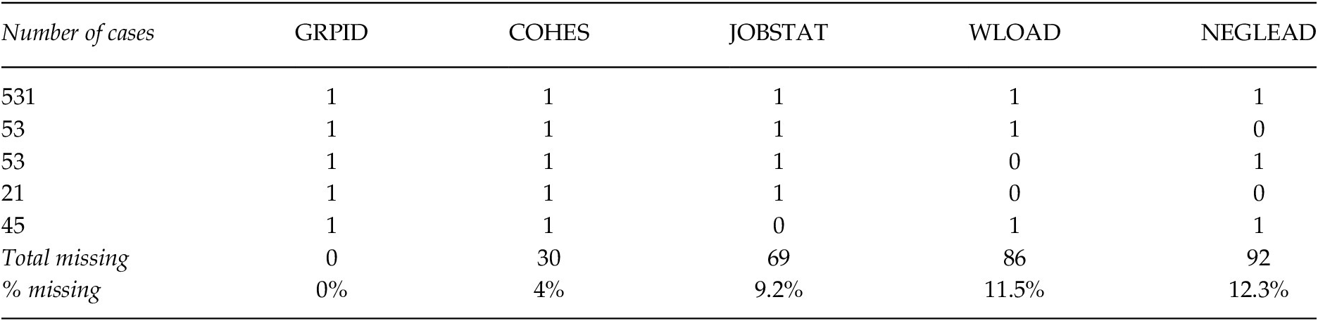
We will find out how many patterns we have without excluding variables. The first column contains the number of cases for each pattern (for example, 531 cases for the first pattern). The next columns inform whether the variable is present (with 1 code) or missing (with 0 code). There are five distinct patterns, the first one with 531 cases represent complete cases, the second show 53 cases with complete variables except NEGLEAD, and so on. The lasts two rows in the Table 4 show total missing data cases in each variable (and the percentage). As can be seen, some of those percentages exceed the maximum 5% commented in the guideline that would allow us to proceed with a method other than MI (such as listwise deletion).

TABLE 4.

Missing Data Patterns of Leadership Data Set

Note. 1 = Observed; 0 = Missing.

With this command, md.pattern(leadership[ , –3]), the researcher can examine each pattern excluding the variable placed in third position (COHES). In addition, with the command md.pairs(leadership) (output is not shown), one can see how many cases exist in the database for each pair of variables. If the reader run this command, he will see, for example, that there are jointly 658 observed cases for the pair (JOBSTAT, COHES) or that there are jointly 594 cases observed for the pair (WLOAD, NEGLEAD) and so on.

Step 3. ICC

We will now examine the intraclass correlation coefficient (ICC) for the outcome variable, JOBSAT (invoking multilevel library). The ICC is used to know whether we have to take into account the multilevel cluster structure during the imputation. JOBSAT variable has an ICC = .129.

• Nulmodel=lmer(JOBSAT ~ 1 + (1|GRPID), data = leadership)

• summary(nulmodel)

ICC is calculated as random intercept variance / (random intercept variance + Level–1 residual variance) = .129. Because of ICC > .10, since missing data affects covariates (and thus it is not recommended using FIML method) and since there are variables with a missing data ratio greater than 5%, the strategy for dealing with missing values is MI.

Step 4. Imputation and Convergence

It will be extended a little more in this step, since it represents the main objective of the article.

Imputation: To make JM imputation we will use jomoImpute( ) function from mitml package. This function has a method called type. This method is important because it establishes the imputation model. This type coding scheme uses the following codes to be assigned to the variables of the imputation model:

1. 1: Variables with missing data that we want to impute receive 1 code (i.e., variables which are outcome variables in the imputation model).

2. 2: Variables completely observed (without missing data) that we want to be fixed effect predictors in the imputation model receives 2 code (i.e., auxiliary variables with fixed effects).

3. 3: Variables completely observed (without missing data) that we want to be random effect predictors in the imputation model receives 3 code (i.e., auxiliary variables with random effects).

1. –1: Grouping variable (their imputation is done separately from the rest of variables). For example, if we want two different imputation models for gender variable (one for male and one for female), this variable would receive –1 code.

2. –2: This code specifies cluster indicator variable (ID Level–2 variable that identifies each cluster). In our example this variable is GRPID.

3. 0: Variables not taking into account in the imputation model (with 0 code we omit these variables from the imputation model).

Note that each code correspond with the position the variables are in the file (so the first code refers to the first variable, GRPID, the second with JOBSAT variable, and so on). For our example, we should use the following codes:

• R> type.L1 <- c(–2,1,0,1,1) # Level–1 imputation model

• R> type.L2 <- c(–2,0,1,0,0) # Level–2 imputation model

• R> names(type.L1) <- names(type.L2) <- colnames (leadership)

• R> type <- list(type.L1, type.L2)

• R> type

type.L1 contains the codes for the imputation model for Level–1 variables and type.L2 contains the code for the imputation model for Level–2 variables (in our example, WLOAD variable). The next command executes the JM imputation algorithm.

• R> imp <- jomoImpute(leadership, type=type, random.L1='full', n.burn=5000, n.iter=1000, m=10)

The first argument includes the file name (leadership). The second one, the type argument (we called it type). The third argument, random.L1='full', let heteroscedasticity for within-cluster variances (instead, random.L1='mean' estimates a unique within-cluster variance). n.burn argument specifies the number of iterations before generating the first copy (data set) and n.iter the number of iteration between two consecutive imputed data sets. The m argument specifies the number of imputed databases generated by the algorithm (10 in our example). It may take one or two minutes to execute this function. jomoImpute( ) provides an imp object (from a class mitml) that, among other things, contains the 10 imputed data sets.

Convergence: In mitml, there are two options for assessing the convergence of the imputation procedure. First, the summary( ) function (see below) with imp object as argument, calculates automatically the potential scale reduction (PSR) index for each parameter in the imputation model. If this value is noticeably larger than 1 for some parameters (say > 1.05), a longer burn-in period may be required. In our case, it would not be necessary a longer period because the main parameters have a reasonable PSR. Executing this command:

• R> summary(imp)

• The output is:

where Beta and Beta2 parameters (i.e., fixed intercepts and coefficients respectively) have PSRs < 1.05, Psi parameters (Level–2 random parameters) has also a PSR < 1.05 and Sigma has a mean PSR value of 1.022 (within-cluster variances). Although in the figure we can see a Max PSR = 1.200 for one Sigma parameter, is not a concern since error variances are estimated for each group and is not a substantive parameter of the model.

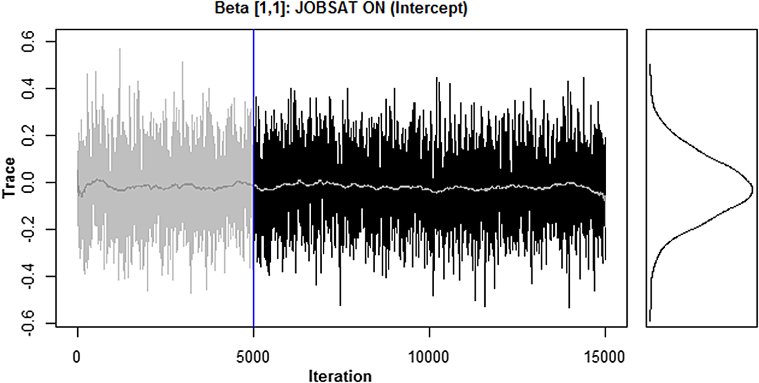
Second, mitml library allows examine the trace plots. We show in Figure 2 the trace plot for parameter Beta[1,1] (i.e., the intercept of JOBSAT).

Figure 2.

Trace Plot (Left) with the Posterior Distribution (Right) of the Intercept Fixed Effect

Note. Graphs for convergence show the estimated parameter value (vertical axe) in each of the imputation dataset (horizontal axe). A criteria for good convergence is that after the burn-in setting (here 5,000 iterations) there is no markedly different trend (as here occurs).

• R> plot (imp, trace ="all", print = "beta", pos =c(1,1))

Taken together, both PSR and the diagnostic plots indicate that the imputation model converged, setting the basis for the analysis of the imputed data sets.

Step 5. Analysis Phase

In order to work with and analyze the imputed data sets, we need to stack the 10 generated (imputed) data sets into a list object. To do so, mitml provides the function mitmlComplete( ) that receives the previously created imp object as an argument.

• R> implist <- mitmlComplete(imp, print="all")

The resulting object is a list containing the imputed data sets. If, for example, the researcher want to examine the imputed values of dataset 2 (not shown), just specify the following command:

• R> implist[[2]]

It is easy to verify that the imputations for variables at Level 2 (COHES in this example) are constant within groups as intended, thus preserving the two-level structure of the data.

In order to obtain estimates for the model of interest, the model must be fitted separately to each of the completed data sets. That is, the analysis model has to be estimated 10 times in this example. The mitml package now offers the function with( ) to fit m statistical models to a list of completed data sets.

It is used the lmer() function from the R lme4 package to fit the model of interest (the analysis model). First, we write in a string the formula of the analysis model (note that this formula follow the rules of the lme4 library):

• R> analysismodel <- 'JOBSAT ~ 1 + NEGLEAD + WLOAD + COHES + (1|GRPID)'

• R> fit <- with(implist , lmer(analysismodel))

The resulting object is a list containing the 10 fitted models (one for each generated copy).

Step 6. Pooling phase

The last step of multiple imputation consists of the pooling phase in which the results of the 10 analysis models are combined into one according with Rubin’s rule (1987). mitml library offers the testEstimates( ) function to pool the results of these models into a unique set of final estimates and standard errors. This is done with the following command:

• R> testEstimates(fit,var.comp = TRUE)

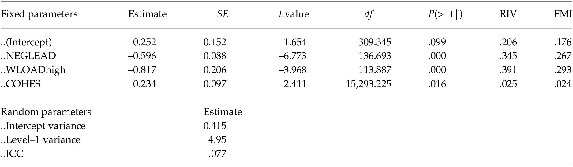
Then, the final model is shown in Table 5.

TABLE 5.

Multilevel Analysis Model Results with MI Via Joint Modeling

The model should be interpreted in the same way as when it is carried out with conventional procedures. There are a significant effect in COHES, WLOAD and NEGLEAD predicting JOBSAT (while cohesion predict an increment in job satisfaction, a negative leadership and work overload predict a reduction in satisfaction). The output of testEstimates includes the final parameter estimates (i.e., the regression coefficients), the MI standard errors, the degrees of freedom and value of the reference t distribution (and its corresponding p-values), the fraction of missing information (FMI), and the relative increase in variance due to nonresponse (RIV). FMI can be helpful for interpreting the results and understanding problems with the imputation procedure. Setting an insufficient number of imputed data sets would lead to an FMI > 0.50 and, consequently, an overestimated standard errors.

Fully Conditional Specification with Mice Method

For applying FCS method we propose to use mice R package (van Buuren & Groothuis-Oudshoorn, Reference Buuren and Groothuis-Oudshoorn2011) and its micemd (Audigier & Resche-Rigon, Reference Audigier and Resche-Rigon2018) plugging. Remember from Software section that there are extensive simulation studies that recommend impute from FCS framework in multilevel models with random slopes or with cross-level interaction effects. As we know, FCS imputes each incomplete variable with a different method depending on the metric of this variable. The mice( ) imputation function, then, may impute continuous, ordinal, nominal or counts variables and the plugging micemd abilities mice( ) function to make FCS multiple imputation strategy in Level–1 and Level–2 data. In addition, this plugging includes methods for imputing systematic and sporadic missing data patterns.

Example 2. Random Slope Model

In this example, it is shown a multilevel imputation of an intercept and slope random model with categorical and continuous variables (Level–1 and Level–2 variables with missing data). Again, we will use leadership data set from the mitml library:

The analysis model will use JOBSAT as the dependent variable predicted by COHES, WLOAD and NEGLOAD. It is modeled random slopes for NEGLEAD (a covariate with missing data).

Applying the guideline for FCS MI methods (see Table 2), we will use 2l.jomo method to impute binary variable WLOAD and 2l.glm.norm method to impute continuous variables (JOBSAT, NEGLEAD, and COHES). Remember that leadership file has 50 clusters with 15 Level–1 units (persons) per cluster.

Again, a distinction must be made between the analysis model and the imputation model

Analysis Model/Research Model

$$ {\mathrm{JOBSAT}}_{ij=}{\beta}_0+{\beta}_1\left({COHES}_j\right)+{\beta}_2\left({WLOAD}_{ij}\right)+{\beta}_3\left({NEGLEAD}_{ij}\right)+{\mu}_{0j}+{\mu}_{1j}\left({NEGLEAD}_{ij}\right)+{\varepsilon}_{ij} $$

Imputation Model

Each incomplete variable is imputed according with its metric and is used all variables of the dataset. That is, the model is accommodated to variable metric.

The imputation method for JOBSAT is 2l.glm.norm. It is used the rest of variables, COHES, NEGLEAD and WLOAD like predictor variables with fixed effects and random effects.

The imputation method for COHES is 2l.glm.norm. It is used the rest of variables, JOBSTAT, NEGLEAD and WLOAD like predictor variables with fixed effects and random effects.

The imputation method for NEGLEAD is 2l.glm.norm. It is used the rest of variables, COHES, JOBSTAT and WLOAD like predictor variables with fixed effects and random effects

The imputation method for WLOAD (a binary variable) is 2l.jomo. It is used the rest of variables, COHES, JOBSTAT and NEGLEAD like predictor variables with fixed effects and random effects

R code: It is necessary to install the following packages as well as to load the following libraries:

• R> install.packages("mitml"); install.packages("lme4"); install.packages ("mice"); install.packages("micemd"); install.packages("lattice"); library(mice); library (micemd); library(lattice); library(lme4); library (mitml);

• We read the leadership dataset from mitml library

• R> data()

• R> attach(leadership)

• R> str(leadership)

The first three steps are the same as in the previous example, so the results are not shown again.

Step 1: Descriptive Analysis

• R> dim(leadership)

• R> summary (leadership)

Step 2. Exploring Missing Data

We do not show again, but reader can see Table 3 for descriptive statistics and Table 4 for missing data patterns from previous example.

• R> md.pattern(leadership)

Step 3. ICC

JOBSAT variable has an ICC = .129. Because of ICC > .10 we will use multiple imputation model. The same reasons of the previous example, lead this one to take the decision to carry out MI to manage missing values.

Step 4. Imputation and Convergence

Again, this step will be covered extensively, since it represents the main objective of the article.

Imputation: Within FCS framework with mice( ) function, we need to specify the imputation model for each imputed variable by assigning which predictors are used to impute it and which method will be used for each variable (e.g., 2l.glm.norm, etc.). For the choice of the predictors of each variable we need to specify a function called predictorMatrix. To choose which method to impute each variable with, we need to use a function called method. Both are passed as arguments within the mice( ) function. It should be note that mice( ) function automatically ignores complete (without missing values) variables in this step.

Therefore, the predictorMatrix( ) procedure are used to declare the predictor variable set. First of all, we set the arguments for predictorMatrix( ) function and to access this function is necessary to initialize a mice object with the default settings:

• R> temp<-mice(leadership,m=1,maxit=0)

temp is a mice object. To access to its predictorMatrix( ) function we use this command:

• R> temp$predictorMatrix

This command returns this output:

In the matrix above, row variables are target variables, that is, variables that are going to be imputed. Column variables are predictors of the target (row) variables. A value of 1 indicates that the column variable is a fixed effect predictor to impute the target (row) variable, and a 0 means that column variable is not used to predict row variable (in the diagonal there are zeros because a variable does not impute itself). We have to accommodate the codes in this predictor matrix according to the imputation model we want. The codes for the predictorMatrix in mice are:

1. –2: This code specifies cluster indicator variable (ID Level–2 variable that identifies each cluster). In our example this variable is GRPID.

2. 0: The column variable do not impute the target (row). For example, for completely observed variables (as GRPID), a vector row with 0s should be set (since this variable does not need to be imputed).

3. 1: This code uses a column variable as a fixed effect predictor to impute the target (row).

4. 2: This code uses a column variable as a random effect predictor to impute the target (row).

5. 3: This code uses a column variable as a fixed effect predictor + aggregated fixed effect predictor to impute the target (row). This preserves contextual effects.

6. 4: This code uses a column variable as a random effect predictor + aggregated fixed effect predictor to impute the target (row). This preserves contextual effects.

For our commodity, all predictor variables are random effects variables because variables with random effects also include fixed effects. Assuming that there are no contextual effects (3 and 4 codes), the matrix to be generated is:

• 

R code to get the above matrix is:

• R> temp$predictorMatrix[,"GRPID "] <- –2 #id cluster variable

• R> temp$predictorMatrix["GRPID ","GRPID "] <– 0

• R> temp$ predictorMatrix [temp$pred==1]<– 2

• R> temp$predictorMatrix

We assign the predictorMatrix( ) function to an object that will be passed as an argument in the mice( ) function:

• R> pred<-temp$predictorMatrix

Now, we will specify the methods according with the guideline using the method( ) function. We will use find.defaultMethod( ) function from Audigier and Resche-Rigon (Reference Audigier and Resche-Rigon2018) micemd plugging:

• R> ind.clust<–1 #this indicates the cluster-id variable

• R> meth<-find.defaultMethod(leadership,ind.clust)

• R> print(meth)

• 

The methods assigned to each variable are those recommended in the guide (see five step of our guide and Table 2).

As proposed in the fourth step of the guide, with FCS imputation it is convenient to pay attention to the order in which the variables are imputed. The vis() method gives us the order in which the variables. Therefore, by writing temp$vis() instruction you can see that the current order es GRPID, JOBSAT, COHES, NEGLEAD and WLOAD (i.e. the order of the variables in the dataframe). To modify the order we can set vis = c(5, 4, 3, 2, 1)) so that first the fifth variable is imputed (this is WLOAD, the most ratio of missing data), then the fourth, etc (see Table 4).

Now we are ready to carry out the imputation phase with mice( ) function via FCS multiple imputation. The first argument of mice( ) function contains the dataframe (leadership), the second the predictionMatrix( ) function, the next contains the method( ) function, the next (vis) the visiting scheme, and the last argument contains the number of generated copies that we want (it may take 10 or more minutes to execute this function and this is done with by-default maxit argument to run the maximum number of iterations):

• R> imp <- mice(leadership, predictorMatrix = pred, vis = c(5, 4, 3, 2, 1)), method = meth, m = 10)

To check convergence it can be used plot( ) function. This provides a plot of the estimated parameters (mean and standard deviation) of the imputed values against the iteration number. For example, the estimated mean and standard deviation for imputed values of the dependent variable JOBSAT:

• R> plot(imp, c("JOBSAT"))

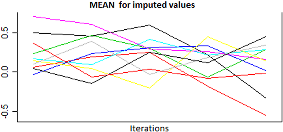
Figure 3 do not show convergence problems for the imputed means of the dependent variable.

Figure 3.

Mean of the Imputed Values via FCS with Gibbs Sampler Algorithm of the JOBSAT Variable in Each Iteration

Note. Graphs for convergence show the estimated parameter value (vertical axe) in each of the imputation dataset (horizontal axe). A criteria for good convergence is that the lines are intermingled across the graph from different MCMC imputation chains (ten in the current example represented by 10 lines).

Step 5. Analysis Phase

As we did in the previous JM example, to work with and analyze the imputed FCS data sets, we need to stack the 10 generated (imputed) data sets into a list object. To do so, mitml provides the function mids2mitml.list ( ).

• R> implist <- mids2mitml.list(imp, print="all")

The resulting object is a list containing the 10 imputed data sets. Then, we create an object with the analysis model formula that will be passed as a parameter to the lmer( ) function of the lm4 library.

• R> analysismodel <- JOBSAT ~ COHES + WLOAD + NEGLEAD + (1 + NEGLEAD|GRPID)

Finally, the analysis phase conclude analyzing the 10 copies separately. This can easily be done with the with( ) function of the mimtl library.

• R> fit <- with(imp,lmer(analysismodel))

The resulting object is a list containing the 10 fitted models (one for each generated copy).

Step 6. Pooling Phase

The results are combined according with Rubin’s rule (1987). mitml library offers the testEstimates( ) function to pool the results of these models into a unique set of final estimates and inferences. This is done with the following command:

• R> testEstimates(fit,var.comp = TRUE)

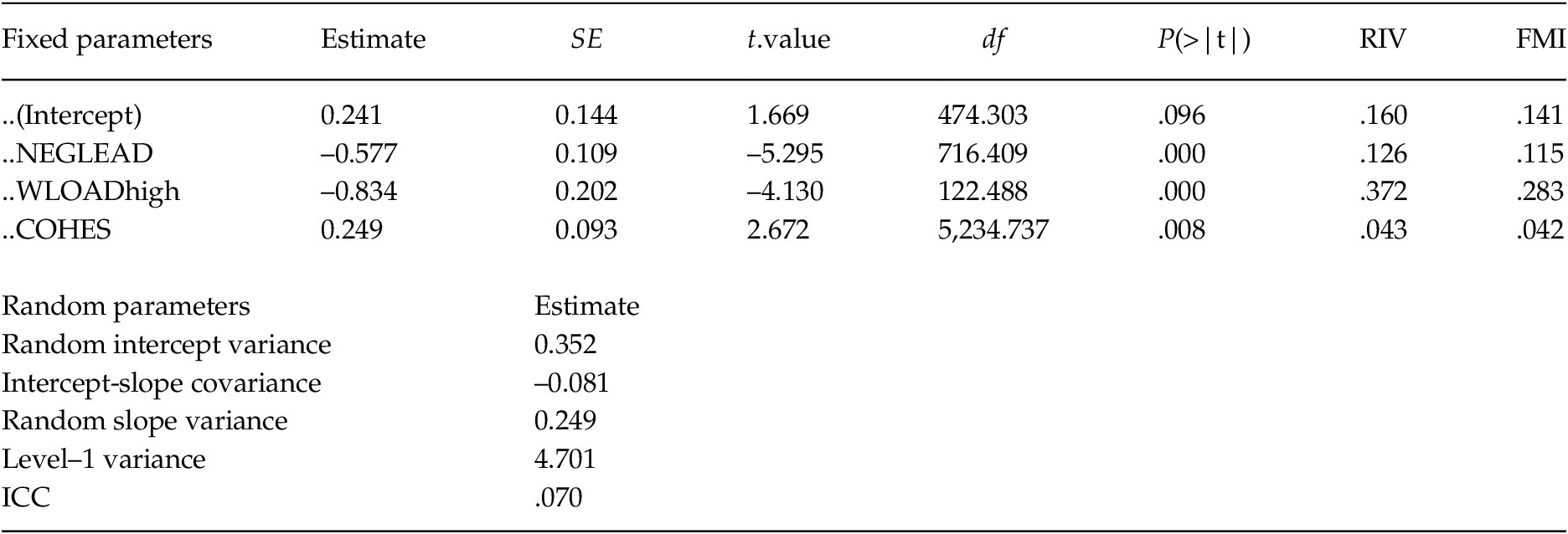
Then, the final model is shown in Table 6.

TABLE 6

Multilevel Analysis Model Results with MI Via Fully Conditional Specification

The model should be interpreted in the same way as when it is carried out with conventional procedures. The difference between this and the previous model is very small (the estimated fixed effects are similar to those estimated with JM framework). Now, random parameters include random slope variance and the covariance between random intercepts and random slopes. These parameters are best estimated from an FCS strategy according to the literature reviewed. As previously, there are a significant effect in COHES, WLOAD and NEGLEAD predicting JOBSAT. The output of testEstimates includes the final parameter estimates, the MI standard errors, the degrees of freedom and value of the reference t distribution (and its corresponding p-values), the fraction of missing information (FMI), and the relative increase in variance due to nonresponse (RIV). The researcher can see the similarity between the results of the model estimated with JM and the one estimated here with FCS.