


Introduction
The subsolidus creep of ice is a major process controlling the flow of glaciers and the shape of large ice sheets (Reference PatersonPaterson, 1969; Reference Sugden and JohnSugden and John, 1976). The velocity and temperature fields in the ice are strongly coupled because the strain-rate of subsolidus creep depends on the exponential of the inverse absolute temperature, while shear in the flow field produces heat by viscous dissipation. Such strong non-linear coupling results in non-uniqueness in the steady solutions and finite-amplitude thermal instabilities of the ice flows. In this paper we use simple, one-dimensional models both to investigate the multiple steady states of deforming ice sheets and their stability. This multiplicity of steady-state solutions and the issue of stability are also encountered in areas of solid-earth geophysics (Reference MeloshMelosh, 1976; Reference Yuen and SchubertYuen and Schubert, 1977; Reference Schubert and YuenSchubert and Yuen, 1978), plasma physics (Reference Dobrott, Dobrott, Miller and RawlsDobrott and others, 1977), chemical reactors (Reference ArisAris, 1975), and chemical physics (Reference Procaccia and RossProcaccia and Ross, 1977)- The review by Reference Clarke, Clarke, Nitsan and PatersonClarke and others (1977) summarizes the previous work on this glaciological problem. A recent paper by Cary and others (1979) also deals with glacier stability. We consider here only the gravitational sliding of a constant-thickness ice sheet with no ablation or accumulation since this situation lends itself to a rigorous, self-consistent, analytic determination of temperature and velocity.
Theoretical Model
We consider a horizontally infinite sheet of ice with constant thickness h on a surface inclined at angle α with respect to the horizontal. The base of the ice sheet is at y = 0, the surface is at y = h. The ice deforms under its own weight and creeps down-slope, in the x-direction, with a steady velocity u. The velocity of the ice sheet parallel to its bed u is a function only of the coordinate normal to the bed y. There is no motion either perpendicular to the basal plane or in the direction normal to x and y. Accordingly, our simplified, one-dimensional, gravitational-sliding model docs not include effects of ablation or accumulation of ice, processes responsible for the overall material balance of large ice masses (Reference PatersonPaterson, 1969).
Consistent with our steady, one-dimensional model, the temperature T in the ice sheet is assumed to depend on y only. Geothermal heat entering the base of the ice sheet and frictional heat generated by the shearing motion of the ice contribute to warming the ice above its surface temperature T 0. One of our primary objectives in this paper is to assess the importance of frictional heating in raising the temperature of the ice and facilitating its deformation. Thus we concentrate on the construction of self-consistent temperature and velocity profiles albeit with a simplified model which cannot account for many of the other physical processes known to influence glacial motions.
The equations governing the temperature and creep of the ice are


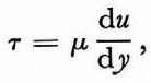

In the force balance Equations (1) where inertial terms have been neglected, т is the shear stress parallel to the base of the ice sheet (defined in Equations (3) in terms of the viscosity µ and the velocity gradient), ρ is the density of the ice, g is the acceleration of gravity, and g sin α is the gravitational force per unit mass parallel to the basal plane. The temperature Equations (2) expresses a balance between heat conduction perpendicular to the basal plane (k is the thermal conductivity of ice) and frictional heating. The formula for the viscosity given in Equations (4) assumes a power-law dependence between strain-rate and stress (strain-rate α T3 (Reference Weertman, Whalley, Whalley, Jones and GoldWeertman, 1973)); the creep of ice is also a thermally activated process with activation energy E* (A is a material constant which depends strongly on the particular deformation mechanism and R is the universal gas constant) (Reference HobbsHobbs, 1974)-
Equations (1) can be integrated directly with the result

where we have assumed т = 0 at the surface. The shear stress increases linearly with depth below the surface of the ice, reaching the maximum value pgh sin α at the base. By substituting for viscosity and shear stress from Equations (4) and (5), we can rewrite the temperature equation as

Equations (6) is solved subject to the boundary conditions


where q b, is the heat flux entering the base of the ice sheet.
Once T is determined from Equations (6) to (8), the velocity profile in the ice sheet can be found by integrating

subject to the condition

The velocity we find from Equations (9) and (10) pertains only to the subsolidus creep of the ice sheet; a constant basal slip velocity can be superimposed on the entire creep velocity profile.
The procedure described above is straightforward if h is considered known a priori. However, the nature of the solutions is such that an alternate approach is useful from a computational point of view. In this alternative scheme we specify the surface velocity u0 , i.e.

resulting in four conditions (Equations (7), (8), (10), and (11)) to be satisfied by our coupled first- and second-order differential equations (Equations (6) and (9)). The additional condition allows determination of h. Thus, one can specify h and compute u 0 from Equations (6) to (10), or one can specify u 0 and compute h from Equations (6) to (11). We will see that u 0 is a multiple-valued function of h whereas h is a single-valued function of u0 . This characteristic of the solutions makes it easier, computationally, to choose u0 and determine h rather than vice-versa. The surface velocity u0 is actually the change in velocity across the ice sheet due to subsolidus deformation. The actual surface velocity of an ice sheet could be considerably larger due to basal slip.
If our problem were cast into dimensionless form, then u/u 0 and T/T 0 would be universal functions of y/h depending only on the four dimensionless parameters

Thus we can write

If T b is the basal temperature (T b = T(y = 0)), then we can also write

These relations allow the numerical results presented later in the paper to be extended to sets of parameter values we have not considered. In presenting our results in the following sections, we will use the dimensional quantities as the ones most readily understandable to the glaciologist.
Parameter Values and Method of Integration
The physical constants used in most of our calculations are summarized in Table I. The rheological parameters E * and A are taken from Reference Clarke, Clarke, Nitsan and PatersonClarke and others (1977). Since these values are derived from single-crystal measurements (Reference Weertman, Whalley, Whalley, Jones and GoldWeertman, 1973), we will vary both E * and A in order to investigate the possibility of placing constraints on the creep properties of poly-crystalline ice in a natural environment. The value of T0 is characteristic of the cold environs of Antarctica; we also consider T0 = 250 K which is a typical value for temperate glaciers (Reference PatersonPaterson, 1969). The basal heat-flow value should be characteristic of continental shield regions (Reference Roy, Roy, Blackwell, Decker and RobertsonRoy and others, 1972). We also use both smaller (qb = 20.9 mW/m2) and larger (qb = 62.7 mW/m2) values of basal heat flux to study the effects of variations in this boundary-condition parameter. For the purposes of emphasizing the effects of viscous dissipation, we have taken a large value of α, 33.5°. We have also considered smaller values of α, 150 and 5°. These values may be found in valley glaciers or near margins of large ice sheets (Reference Sugden and JohnSugden and John, 1976). We will show later how our results can be scaled to even smaller α.

Equations (6) and (9) with the associated boundary conditions, Equations (7), (8), (10), and (11), constitute a two-point, non-linear boundary-value problem. The numerical solution is obtained by downward integration (fourth-order Runge-Kutta method) from y = h, with guesses for dT/dy at y = h and the value of h. These quantities are iteratively adjusted by the Newton-Raphson method until the two boundary conditions, Equations (8) and (10), are satisfied at y = 0. To facilitate the efficient convergence of the numerical solution, we integrated the temperature equation from y = h to the extremely small depth at which T increased by at most 0. 1 K without including the viscous dissipation term. At these small depths we also took u = u0 . At greater depths, the complete equations were integrated. The solutions were acceptable only when the values of dT/dy (y = h) and h were unaffected by decreasing the size of integration steps, usually chosen to be O(10−3 h).
Profiles of Temperature, Velocity, and Viscosity
We show two examples of how temperature, velocity, and viscosity vary with position in the ice sheet. Fig. 1 is for E* = 60.7kJ/mol (14.5 kcal/mol) and Fig. 2 is for E* = 125.5 kJ/mol (30 kcal/mol). In both cases T0 is 218 K, qb is 41.8 mW/m2 (1.0 μ, cal/cm2s), and α = 33.5°. Other parameter values are given in the figure captions. We will see later that the case with low activation energy is an example of a subcritical state while the case with high activation energy represents a supercritical state. The former is characterized by little shear heating and only a small temperature increase through the ice; the temperature profile is essentially linear. In the latter case, frictional heating is more important as can be seen by the curvature in the temperature profile near the base of the ice sheet. Thus, the isothermal approximation (Reference NyeNye, 1957) is quite valid for the subcritical situation. The overall temperature increase in the supercritical case is substantial and approximately the lower 60% of the sheet is at temperatures above the melting point of ice (melting temperature versus depth is shown by the dotted line). The ice sheet is only about 110 m thick in the subcritical case whereas it is about 1.9 km thick in the supercritical case.
Depth profiles of temperature T, velocity u, and effective viscosity μ. The parameter values are those given inTable I.

T, u, and μ versus depth in the ice sheet. The parameter values are those given in Table I except for E* which has the high value 125.5 kJ/mol (30 kcal/mal). The dotted line is the depth profile of the melting temperature taken from Reference Sugden and JohnSugden and John (1976)

The surface velocities for both values of E * are identical, u 0= 1 m/year. However, for the smaller value of E* the shear occurs over about the lower 70% of the ice sheet whereas for the higher value of E* , the shear is confined to about the lower 25% of the ice sheet. The velocity profile of Reference NyeNye (1957) is qualitatively similar in appearance to the one for the lower activation energy. There are large variations in viscosity throughout the ice layer. For the subcritical case, μ decreases by more than two orders of magnitude over the lower 90% of the ice sheet while for the supercritical case the decrease is eleven orders! Since the surface shear stress is zero, the effective viscosity as defined by Equations (4) is infinite at the surface. Near the surface where there exist crevasses the deformation cannot be described by a viscous model. Thus the mathematical singularity in the surface viscosity has no physical significance. The much larger viscosity variation between the near-surface and the base of the ice sheet in the supercritical case is the result of the relatively large value of E * for this case.
Surface Velocity, Basal Temperature, and Ice Thickness
The overall character of an ice sheet is well described by giving its thickness h, surface velocity u0 and basal temperature Tb = T (y = 0) for the many different environmental circumstances under which the ice sheet can exist. The environmental parameters include surface temperature T0, basal slope α, and basal heat flux qb . In addition, it is of interest to describe how these basic characteristics of ice sheets depend on the rheological properties of the ice.
Figures 3 and 4 show how h, u0 , and Tb, vary with creep activation energy for T0 = 218 K, α = 33.5°, and q b = 41.8 mW/m2 (1 μcal/cm2 s). u0 and Tb are seen to be double-valued functions of h in the range of u0, h considered. This multiplicity of steady solutions is well known in both fluid dynamical (Reference JosephJoseph, 1964) and chemical engineering (Reference Gavis and LaurenceGavis and Laurence, 1968) literature. Reference Clarke, Clarke, Nitsan and PatersonClarke and others (1977) have shown that there are in fact three possible values of T b for certain ice-sheet thicknesses. They integrated the temperature equation only and discussed the solutions in terms of the multiplicity of values of the surface temperature gradient. It is important to simultaneously integrate the rheological equation and consider the multiplicity of values of the surface velocity. As an observable, u0 can place useful constraints on dynamical models of glaciers. It is equally important to consider the multiplicity of T b values since subsolidus deformation models are meaningful only when the temperature rise through the ice does not lead to melting.
Surface velocity u0 versus ice thickness h. Except for the values of E* which are indicated on the figure, all parameters have the values given in Table 1. The results can be extended to arbitrary α following the discussion in the text.

Basal temperature T b as a function qf ice thickness h. The dotted line is the temperature at which melting occurs at the base of an ice sheet of thickness h. Parameter values are those given in Table I except for the indicated values of E*. The results can be extended to arbitrary α following the discussion in the text.

The critical values u0 *, h* , and Tb *, h* are the points on Figures 3 and 4 which separate the curves into two branches. On the upper or supercritical branch, u 0 and T b decrease with increasing h, while on the lower or subcritical branch, u0 and T b increase with increasing h. There is a third branch on which u0 and T b also increase with h, but along this branch u0 and T b are so large that the solutions are not physically meaningful. If we ignore this third branch, then there is a maximum steady thickness, namely h* , that can be attained by an ice sheet creeping down-slope under its own weight. The existence of a critical thickness h* opens the possibility of instability when, for example, a sudden climatic deterioration lasting say O(102) years, produces a layer of ice thicker than h* . We discuss the stability of these one-dimensional, steady subsolidus creep models in a later section.
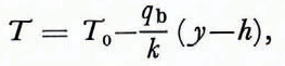
The solutions which lie along the subcritical branch far from the critical point represent states in which there is relatively little shear deformation and relatively little hearing by frictional dissipation. In these cases, the temperature profile in the ice is essentially linear
and
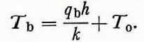
In addition, qbh/kT0 is much smaller than unity under these circumstances and the basal temperature is only slightly higher than the surface temperature. With qbh/kT0 ⪡ 1 and T given by Equations (12), one can obtain an approximate formula for u 0 by integrating Equations (9); the result is

where

Only for those states lying near the critical point or on the supercritical branch does frictional dissipation contribute substantially toward heating the ice. Fig. 4 shows that the basal temperatures of most of the supercritical states exceed the melting point of ice while those of most of the subcritical states lie below the melting point. However, for the low activation energies E* = 60.7 kJ/mol (14.5 kcal/mol) and E* = 94.1 kJ/mol (22.5 kcal/mol) there are supercritical states which do not entail any melting of the ice, while for the high activation energies E* = 125.5 kJ/mol (30 kcal/mol) and E* = 156.9 kJ/mol (37.5 kcal/mol) there are subcritical states which involve melting. For these same high activation energies, u0 for the subcritical states does not exceed about 10−2 m/year (Fig. 3). Even for E* = 94.1 kJ/mol, u0 * is only about 10−1 m/year. Only for the lowest activation energy is it possible for the subcritical states to achieve surface velocities of several meters per year. However, for E* = 60.7 kJ/mol, h* is only about 150 m.
In summary, for the values of surface temperature, basal slope, basal heat flux, and rheological parameters used in Figures 3 and 4, there are no subcritical states (or supercritical ones for that matter) which simultaneously satisfy the requirements of no melting, surface velocities of the order of meters per year, and ice thicknesses of hundreds of meters, at the two highest values of E* considered. These requirements can only be met by supercritical solutions for E* = 94.1 kJ/mol. For E* = 60.7 kJ/mol, all of the above requirements can be satisfied by a limited number of subcritical and supercritical states; however, these states lie very close to the critical point making them vulnerable to frictional-heating instability by finite-amplitude perturbations. Reference Clarke, Clarke, Nitsan and PatersonClarke and others (1977) have argued that the supercritical states are not attainable by real glaciers. Our stability analysis, which we discuss later, indicates that the supercritical states, if they exist, are at least stable to small amplitude perturbations.
Can the above conclusions be modified by using different values of q b, T 0, A, or α? Figures 5 and 6 show how variations in A affect u 0 and T b for the smallest and largest values of E* used in the previous figures. Changing A by six orders of magnitude has little effect on the graph of u0 versus h at the high activation energy. At the low value of E* , however, a decrease in A by three orders of magnitude reduces u 0 * by about a factor of ten while it increases h* to about 400 m. An increase in A by three orders of magnitude at the low value of E* increases u0 * by about an order of magnitude but it decreases h* to only about 50 m. The surface velocity requirement is facilitated by an increase in A while the thickness requirement is aided by a decrease in A. These wide variations in A do not alter the fact that there are supercritical states at the low value of E* which do not involve melting while there are subcritical states at the high value of which are molten.
Surface velocity u0 versus ice thickness h. The figure illustrates the effects of variations in the rheological parameter A which had the value given in Table I. This value was both increased and decreased by a factor of 103 to generate the curves shown. Aside from the values specified in the figure, all parameters had the values given in Table 1. The results can be extended to arbitrary α following the discussion in the text.

Effects of rheological parameter variations on the relation between the basal temperature Tb and ice thickness h. The melting point is indicated by the dotted curve. Parameter values are given in Fig. 6. The results can be extended to arbitrary "following the discussion in the text.

Figures 7 and 8 illustrate the influence of qb on the critical points. Even a variation in basal heat flux by a factor of three has little effect on the parameters u 0*, Tb * and h* at E* = 60.7 kJ/mol. At twice this value of the activation energy, the same variation in q b still produces very small changes in u0 * and Tb *. However, the changes in h* are more substantial. Increasing qb leads to a reduction in h* , an increase in Tb * , and an increase in u0 * .
Influence of basal heat flux qb on the relation between surface velocity u0 and ice thickness h. Parameters not specified in the figures are given in Table 1. The curve for qb = 41.8 m W/m2 and E* = 60.7 kl/mol lies in the darkened region. The results can be extended to arbitrary α following the discussion in the text.

Basal temperature Tb versus ice thickness h for variations in qb. Parameters are given in Table I if not specified on the figure. The curve for qb = 41.8 m W/m2, E* = 60.7 kl/mol is in the darkened region. The results can be extmded to arbitrary α following the discussion in the text

Surface temperature variations are investigated in Figures 9 and 10. A higher surface temperature characteristic of a temperate glacier produces somewhat larger values of u0 * and Tb * , and a smaller value of h* . Even with a warm surface temperature, there are still supercritical states (for E* = 60.7 kJ/mol) that involve no melting and subcritical states (for E* = 125.5 kJ/mo1) that do.
Effects of surface temperature T0 on the relation between surface velocity u0 and ice thickness h. Parameten not given in the figures are in Table I. The results can be extended to arbitrary α following the discussion in the text.

Influence of surface temperature To on basal temperature Tb and ice thickness h. The dotted curve is the melting point curve. Parameters are the same as in Figure 9. The results can be extended to arbitrary αfollowing the discussion in the text.

Effects of basal slope variations are shown in Figures 11 and 12. A decrease in α results in little change in either u0 * or Tb *. However, h* increases substantially with decreasing α. The thickness constraint becomes much easier to meet for E* = 60.7 kJ/mol at slope angles less than ten degrees.
Effects of basal slope α variations on surface velocity and ice thickness. Unspecified parameters are listed in Table I. The results can be extended to arbitrary α following the discussion in the text.

Our numerical results can be extended to glaciologically relevant small values of α of order 1° as follows. Consider the diagrams of u0 versus h. Since the subcritical states involve relatively little frictional heating, the dependence of u0 on α is essentially given by

(see either Equations (12) or (16)). The validity of this dependence can be verified in Figure 11; the subcritical states for fixed E* and h lie along parallel lines shifted vertically with respect to each other according to u0 * sin3 α. This dependence can be used to extend the subcritical results of Figures 3, 5, 7, 9, and 11 to arbitrarily small α. The basal temperature of the subcritical states is essentially independent of α. (see Equations (15) or Figure 12).
Relations between basal temperature Tb and ice thickness h for different basal slopes α. The dotted curve is the melting-point curve. Parameters are the same as in Fig. 11 The results can be extended to arbitrary α following the discussion in the text.

Since the supercritical states are dominated by frictional heating, the dimensionless parameter qb, h/kT0 has relatively little influence on Equations (12) and (13). This can be seen in Figures 7 and 8 which show the effects of varying q b on the u0 versus h and T b versus h characteristics of the basic states. Given the relative unimportance of this dimensionless ratio, it is clear from Equations (12) that if we scale h according to

and u 0 according to

then we can determine the relation between u0 and h for supercritical states for arbitrarily small α. If this relation is of the approximate form

for given α and other parameters, then the relation corresponding to another value of α, α’ say, is

The validity of Equation (Equations (19) for the supercritical states can be verified from the results of Fig. II. From Equations (13), it can be seen that if we scale h according to

then Tb for the supercritical states is unchanged so long as basal heating is relatively unimportant. The validity of this result can be verified in Figure 12.
By rescaling the subcritical and supercritical states according to the above, one can estimate how u 0 *, h *, and Tb * change with variations in α.
The overall conclusions we reached after examining Figures 3 and 4 are essentially unaltered by our exploration of variations in qb, T0, A, and α. In the next section we discuss the stability of these steady solutions.
Stability of Steady Solutions
We have conducted both one-dimensional and two-dimensional stability analyses of a number of our supercritical steady solutions. In the one-dimensional analysis, the temperature perturbation equation is identical to the one employed by Reference Clarke, Clarke, Nitsan and PatersonClarke and others (1977) (their equation (23)). We solved this equation using the numerical methods described in Reference Yuen and SchubertYuen and Schubert (1977). The smallest eigenvalue of the second-order system is identified by the absence of interior nodal points of the associated eigenfunction. The equations and boundary conditions for the two-dimensional perturbations are given in the Appendix.
In all the cases examined by both types of stability analysis we found no unstable modes. Table II summarizes the minimum decay times of one-dimensional and two-dimensional disturbances for E* = 125.5 kJ/mol, α = 33.5°, and qb= 41.8mW/m2. Decay times decrease with a decrease in α since there is less viscous dissipation for smaller α. As one approaches the critical point on the supercritical branch, the decay times of the infinitesimal disturbances increase to values comparable to the characteristic lifetimes of large ice masses (Reference LliboutryLliboutry, 1964-65, Tom. 2). Even though linear analyses predict stability, finite-amplitude effects can be destabilizing especially near the critical point (Reference JosephJoseph, 1976).

Summary and Conclusions
Previous models of the gravitational sliding of ice sheets have all been isothermal in character. The velocity and temperature fields were not derived in a self-consistent manner which accounted for the coupling of these fields via the dependence of viscosity on temperature and via frictional heating. In this paper we have concentrated on developing a self-consistent thermomechanical subsolidus model of gravitationally sliding ice sheets and exploring how the basic structures depend on the rheological and environmental parameters. Future calculations should incorporate the important processes of ablation and accumulation which we have not accounted for.
We have found from our numerical experiments with the rheological and environmental parameters that in order to satisfy all the constraints on surface velocity, ice thickness, and melting, activation energies larger than about 100 kJ/mol can be ruled out for both temperate and extremely cold conditions. The creep activation energy of polycrystalline ice has not been measured at low temperatures (Reference HobbsHobbs, 1974). Our results thus provide useful information on the flow law of polycrystalline ice at all temperatures and in particular at T<230 K.
Our linear stability analyses demonstrate that all steady states along both the subcritical and supercritical branches are stable. Since we have not investigated the initial-value problem for the evolution of ice sheets, we cannot address the question of what evolutionary paths can be taken to reach the supercritical branch.
From numerical calculations for the onset of thermal runaways (Reference GruntfestGruntfest, 1963; Reference Griggs, Baker, Mark and FernbachGriggs and Baker, 1969; Reference Fujii and UyedaFujii and Uyeda, 1974), one can readily observe that runaway systems do not grow in a simple exponential manner. Rather, for thicknesses which are slightly (c. 10%) in excess of the critical value for times lasting at least a hundred years, super-exponential growth rates are attained within a few tenths of the characteristic thermal diffusion time. Thus, the linear analysis of Clarke and others (1977) predicts overly conservative growth times for thermal runaways which are caused by a finite change in ice thickness maintained for an indefinite period of time. This is also apparent from the asymptotic analyses of Kassoy (Reference Kassoy1975, Reference Kassoy1977) for the different time scales present in the initiation and subsequent growth of chemical explosions. Thus, we need to re-evaluate the temporal evolution of shear-heating instabilities in ice sheets triggered by finite-amplitude perturbations with realistic time histories (Reference Sugden and JohnSugden and John, 1976). Certain time histories for glacier development may lead to the disintegration of large ice sheets (Reference WeertmanWeertman, 1961), an event having serious climatological and other consequences.
Acknowledgements
We thank Dick Peltier and Andrew Fowler for some provocative conversations concerning this paper. This research was supported by the Earth Sciences Section, National Science Foundation, NSF Grant EAR-77-15198 and by intramural computing funds from the University of California.
APPENDIX
Equations for Two-Dimensional Stability Analysis
The equations for two-dimensional disturbances have already been derived by Reference Yuen and SchubertYuen and Schubert (1979) in their study of frictional-heating stability of shear flows in the Earth’s upper mantle. Here we discuss only the modifications to those equations arising from the different rheologies of mantle rocks and ice and the linear dependence of the basic state shear stress on depth in ice sheets. The equation for the temperature perturbation is identical to equation (20) of Reference Yuen and SchubertYuen and Schubert (1979). The perturbation momentum equation for the complex amplitude of the vertical velocity fluctuation Û is

T denotes the complex amplitude of the temperature perturbation and η is the horizontal wavenumber of the disturbance η = 2π/λ, λ is the horizontal wavelength). The overbar refers to steady-state quantities.
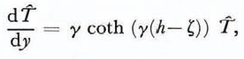
Since there is no viscous deformation in the top portions of the slab, only temperature fluctuations can exist there. We integrate the complete perturbation momentum and temperature equations downward from a depth where ice begins to creep. The boundary condition for the temperature perturbation at this elastic-viscous interface (y = h—ζ) is
where

K is the thermal diffusivity of ice and ĉ is the complex wave velocity of the disturbance. We have also imposed the boundary conditions of zero shear stress and zero vertical velocity at this interface. For further details concerning the equations, boundary conditions, and solution methods, the reader is referred to Reference Yuen and SchubertYuen and Schubert (1979).
Discussion
G. K. C. Clarke: Your suggestion that a finite (non-linear) perturbation analysis might yield explosively-fast growth rates for the perturbation is an interesting one. In our work on creep instability using linear perturbation analysis (Clarke and others, 1977) we tended to discount the importance of creep instability in triggering surges of cold glaciers because we found growth times which were too large to explain surge periodicities of 20-50 years. If your speculation proves true then the question is re-opened.
D. A. Yuen: Yes, we would like to investigate the issue of “the fizzle or the bang” of thermal instabilities when both finite-amplitude perturbations and the length of such perturbation are considered. The possible temporal coupling between the “run-away” time scale and the length of the excitation, such as by a sudden climatic change, is interesting. We hope to provide some quantitative results of this endeavour in the near future.
W. D. Hibler III: How do you use the initial-value-problem approach to obtain multiple steady states. It seems that for the same initial values the time evolution should always be the same.
Yuen : We have solved a steady-state boundary-value problem by taking the time derivative of the temperature to be zero. To obtain multiple steady-state states from an initial-value approach, one must explore the space of initial conditions such that the multiplicity is achieved in the steady state.
W. F. Budd : What happens when your model reaches melting point ? Does it just develop the properties of “temperate” ice?
Yuen: Our model does not include the transition of rheologies between a subsolidus and liquid state. At such a transition the flow field would probably be no longer one-dimensional in character and must be modelled appropriately by a set of two-phase fluid equations, as both phases co-exist at this stage.
J. W. Glen: I am not perturbed by the fact that you found both of your solutions were stable —if they were not we could hardly expect the unstable ones to be observed. With both stable we can have two kinds of flow, just as in hydraulic flow in a channel, and what we need to know is the kind of kick required to move from one to the other—the glacier equivalent of a Russell wave.
Yuen : I am glad that you appreciated the fact that linear stability sometimes predicts stable results. There are cases in fluid mechanics such as the Hagen-Poiseuille, plane Couette flows, where finite-amplitude effects are destabilizing. This fact is commonly associated with the “snap-like” transitions associated with secondary bifurcation of shear flows, very much unlike their convective counterparts.



