





1 Introduction
For positive integers t, v, k and
$\lambda $
 , a t-
$(v, k, \lambda )$
 design, or simply a t-design, consists of a v-set V, whose elements are called points, and a collection B of k-subsets of V, whose elements are called blocks. The defining property of a t-design is that every t-subset of V is contained in exactly
$\lambda $
 blocks. A design is nontrivial if B is not the whole collection of all k-subsets of V.
In 1977, Wilson [Reference Wilson18, Reference Wilson17, Reference Wilson19] constructed
$2$
 -designs for all sufficiently large v under some necessary divisibility conditions. In 1987, designs for all t and some
$v, k, \lambda $
 were first constructed by Teirlinck [Reference Teirlinck15]. In 2014, Keevash [Reference Keevash10] developed the method of randomized algebraic construction, and, in particular, constructed t-designs for all sufficiently large v under the divisibility conditions.
The focus of this paper is on the sizes of designs. Fisher [Reference Fisher9] proved in 1940 that, for nontrivial
$2$
 -designs, the number of blocks is at least the number of points, namely,
$|B| \geq v$
 . This inequality is known as Fisher’s inequality. In 1968, Petrenyuk [Reference Petrenyuk12] generalized Fisher’s inequality and proved that for nontrivial
$4$
 -designs,
$|B| \geq {v \choose 2}$
 . Moreover, Petrenyuk proposed a conjectural inequality
$|B| \geq {v \choose s}$
 for
$2s$
 -designs. In 1975, Ray-Chaudhuri and Wilson [Reference Ray-Chaudhuri and Wilson13] proved Petrenyuk’s conjecture. This lower bound is known as the Fisher type lower bound. Designs that achieve this lower bound are called tight.
Tight
$2$
 -designs are also called symmetric designs. Typical examples are the
$2$
 -
$(n^2 + n + 1, n + 1, 1)$
 designs arising from projective planes of order n, and the
$2$
 -
$(4 n - 1, 2 n - 1, n - 1)$
 designs arising from Hadamard matrices of order
$4 n$
 . For tight
$4$
 -designs, the Witt
$4$
 -
$(23, 7, 1)$
 design and its complement, the Witt
$4$
 -
$(23, 16, 52)$
 design, are tight
$4$
 -designs. No other nontrivial tight
$2s$
 -designs with
$s \geq 2$
 have been found.
Due to a series of works [Reference Delsarte5, Reference Ray-Chaudhuri and Wilson13, Reference Peterson11, Reference Bannai2, Reference Enomoto, Ito and Noda8, Reference Bremner3] in the 1970s by Delsarte, Ray-Chaudhuri, Wilson, Bannai, Peterson, Enomoto, Ito, Noda and Bremner, it was known that (1) the only nontrivial tight
$4$
 -designs are the Witt designs; (2) there are no nontrivial tight
$6$
 -designs; (3) there are only finitely many nontrivial tight
$2s$
 -designs for each
$s \geq 5$
 . Therefore, it was widely conjectured that symmetric designs and the Witt designs are the only nontrivial tight designs.
There was no further progress on this conjecture until recently. In 2013, Dukes and Short-Gershman [Reference Dukes and Short-Gershman6] proved the conjecture for
$s \in \{5, 6, 7, 8, 9\}$
 by extending Bannai’s approach [Reference Bannai2]. In 2018, the author [Reference Xiang20] used a different approach to prove the
$s = 4$
 case.
In this paper, we have completely proved the conjecture by using new strategies.
Theorem 1.1 (Main result).
The only nontrivial tight
$2 s$
 -designs with
$s \geq 2$
 are the Witt
$4$
 -
$(23, 7, 1)$
 design and the Witt
$4$
 -
$(23, 16, 52)$
 design.
In coding theory, the perfect e-code is the dual concept to the tight
$2s$
 -design. Tietäväinen [Reference Tietäväinen16] proved in 1972 that the only nontrivial perfect e-codes with
$e \geq 2$
 on Hamming association schemes over finite fields are the
$[23, 12, 7]_2$
 and
$[11, 6, 5]_3$
 Golay codes. The classification of perfect e-codes on Johnson association schemes, where t-
$(v, k, \lambda )$
 designs reside, is still open. Theorem 1.1 can be viewed as the design theory counterpart of the classification of such perfect codes.
1.1 Intersection numbers and the Wilson polynomials
An important tool in the study of block designs is the set of intersection numbers of the designs. These are the sizes of the intersections of different blocks in a design.
For a tight
$2 s$
 -
$(v, k, \lambda )$
 design, its intersection numbers are completely determined by s, v and k. More precisely, combining the results of Delsarte [Reference Delsarte5] and those of Ray-Chaudhuri and Wilson [Reference Ray-Chaudhuri and Wilson13], for a fixed s, there exists a degree s polynomial
$\Phi _s(v, k; z) \in {\mathbb {Q}}(v, k)[z]$
 in z with coefficients in
${\mathbb {Q}}(v, k)$
 , such that the zeros of
$\Phi _s(v, k; z)$
 are exactly the intersection numbers of a nontrivial tight
$2 s$
 -
$(v, k, \lambda )$
 design. These polynomials
$\Phi _s$
 are called the Wilson polynomials. They are the design theory counterparts of the Lloyd polynomials for perfect codes.
Since the intersection numbers are all integers, so are the zeros of the Wilson polynomials. This gives a necessary condition for the existence of nontrivial tight designs. Most previous work has focused on the behavior of the zeros of the Wilson polynomials.
When
$s = 2$
 or
$s = 3$
 , the zeros of
$\Phi _s$
 can be computed. In 1979, Enomoto-Ito-Noda [Reference Enomoto, Ito and Noda8] analyzed the zeros of
$\Phi _2$
 and proved that the nontrivial tight
$4$
 -designs give integer points on some explicit elliptic curve. Soon after this result, Bremner [Reference Bremner3] and Stroeker [Reference Stroeker14] independently determined all integer points on this elliptic curve, thus proving Theorem 1.1 for
$s = 2$
 . In 1977, Peterson [Reference Peterson11] analyzed the zeros of
$\Phi _3$
 and proved Theorem 1.1 for
$s = 3$
 .
When
$s \geq 5$
 , in 1977, Bannai [Reference Bannai2] obtained the asymptotic behavior of the zeros of
$\Phi _s$
 as
$v \to \infty $
 and showed that they are controlled by the zeros of the Hermite polynomials. Using the properties of the Hermite polynomials, he proved that, for each fixed
$s \geq 5$
 , there are only finitely many nontrivial tight
$2 s$
 -designs. In 2013, Dukes and Short-Gershman [Reference Dukes and Short-Gershman6] applied Bannai’s approach explicitly and proved Theorem 1.1 for
$s \in \{5, 6, 7, 8, 9\}$
 .
Unfortunately, Bannai’s method does not seem to be able to prove Theorem 1.1. It does not apply to the
$s = 4$
 case since the zeros of the degree
$4$
 Hermite polynomial do not satisfy the needed properties. Moreover, for large s, some heuristics by the author suggest that an explicit version of Bannai’s approach might only give a loose upper bound
$v \ll \exp (s)$
 as
$s \to \infty $
 . Remark 5.4 elaborates on why this upper bound is not small enough to prove Theorem 1.1.
In 2018, the author [Reference Xiang20] studied the coefficients of the Wilson polynomials, instead of the zeros of the Wilson polynomials, and thus obtained some different necessary conditions for the existence of nontrivial tight designs. By combining these conditions and results on
$\Phi _4$
 in [Reference Bannai2, Reference Dukes and Short-Gershman6], the author [Reference Xiang20] proved Theorem 1.1 for
$s = 4$
 . However, the results we need on
$\Phi _4$
 are unique to the
$s = 4$
 case, and new ideas are needed to prove Theorem 1.1.
1.2 Strategy and organization
The proof of the main result consists of two parts: showing a good upper bound for v, and showing a good lower bound for v. In both parts, we use some new strategies.
The main idea of proving an upper bound is to construct an auxiliary function H in v and k for each fixed s such that the following three properties hold.
-
(i) The function H takes rational values with bounded denominators at the parameters of nontrivial tight $2 s$
 -designs.
-
(ii) As $v, k \to \infty $
with
$v \geq k$
,
$H = o(1)$
. -
(iii) $H > 0$
.


Since rational numbers with fixed bounded denominators are discrete, (i), (ii) and (iii) conflict with each other when v is sufficiently large compared with s, which leads to an upper bound for v in terms of s.
Such an H is constructed in Sections 2 and 3. There are two families of basic functions
$\lambda _i$
 and
$\alpha _i$
 with
$\lambda _i = O(v^s)$
 and
$\alpha _i = O(v^i)$
 . We first construct certain rational linear combinations
$h_i = O(v)$
 of
$\lambda _i$
 ’s and
$\alpha _i$
 ’s in Section 2. We then construct a certain rational quadratic combination H of
$h_i$
 ’s in Section 3. This H satisfies i because
$\lambda _i$
 ’s and
$\alpha _i$
 ’s do. Moreover, this H happens to have a simple closed-form formula, which allows us to prove
$H = O(v^{- \lfloor s / 2 \rfloor + 2})$
 . Therefore, (ii) holds for
$s \geq 6$
 . The property (iii) also follows from the closed-form formula of H.
In Section 4, we give an upper bound for the denominators of
$H(v_0, k_0)$
 for parameters
$(v_0, k_0)$
 of nontrivial tight
$2 s$
 -designs. This gives an upper bound
$v \ll s$
 as
$s \to \infty $
 . The result in Section 4 relaxes the bounded denominator condition in (i) a little bit, since otherwise we could only prove
$v \ll s^5$
 .
On the other hand, we analyze the parameter
$\lambda $
 to get a lower bound for v. The denominator of
$s! \lambda $
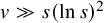
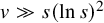
 is a product of consecutive integers, which cannot contain any primes. Using known estimates of prime gaps, we prove
$v \gg s (\ln s)^2$
 as
$s \to \infty $
 in Section 5.
These two bounds prove Theorem 1.1 for sufficiently large s. To give a proof for all
$s \geq 2$
 , we need to get explicit versions of the upper bound
$v \ll s$
 and the lower bound
$v \gg s (\ln s)^2$
 , which is done in Sections 4 and 5, respectively. Section 6 handles the small s cases by giving explicit upper and lower bounds for v. It also contains the full proof of Theorem 1.1.
Notation. The set of all integers in a real interval
$[a, b]$
 is denoted by
$[a, b]_{{\mathbb {Z}}}$
 . The n-th rising factorial and the n-th falling factorial of x are denoted by
$x^{\overline {n}} := \prod _{i = 0}^{n - 1}(x + i)$
 and
$x^{\underline {n}} := \prod _{i = 0}^{n - 1}(x - i)$
 , respectively. We adopt the convention that
$x^{\overline {0}} = x^{\underline {0}} = x^0 = 1$
 . The p-adic valuation of a rational number x is denoted by
$\mathrm {val}_p(x)$
 .
2 Bounded denominators of
$h_{s, i}$
’s

This section studies several families of functions in v and k that take rational values with bounded denominators at the parameters of nontrivial tight designs.
Let
${\mathbb {Z}\mathrm {Val}}[v, k]$
 be the ring of integer-valued rational functions in v and k,
${\mathcal {D}}_s$
 the collection of all
$(v_0, k_0)$
 ’s such that there exists a nontrivial tight
$2 s$
 -
$(v_0, k_0, \lambda _0)$
 design, and
${\mathcal {A}}_s$
 the ring of integer-valued functions on
${\mathcal {D}}_s$
 . Then,
${\mathbb {Q}} \otimes _{{\mathbb {Z}}} {\mathcal {A}}_s$
 is the ring of rational-valued functions on
${\mathcal {D}}_s$
 with bounded denominators. It is clear that
${\mathbb {Z}\mathrm {Val}}[v, k] \subseteq {\mathcal {A}}_s \subseteq {\mathbb {Q}} \otimes _{{\mathbb {Z}}} {\mathcal {A}}_s$
 .
For designs, there are three families of important functions. For each
$i \in [0, s]_{{\mathbb {Z}}}$
 , let


It is well known that
$\lambda _{s, i} \in {\mathcal {A}}_s$
 , since every tight
$2 s$
 -
$(v, k, \lambda )$
 design is an
$(s + i)$
 -
$(v, k, \lambda _{s, i})$
 design. It was proved in [Reference Xiang20, Corollary 2.2] that
$\alpha _{s, i} \in {\mathcal {A}}_s$
 . More precisely, the zeros of the Wilson polynomial in z,

are exactly the s intersection numbers of tight
$2 s$
 -designs by [Reference Delsarte5, Reference Ray-Chaudhuri and Wilson13, Reference Bannai2]. Therefore,
$\alpha _{s, i}$
 must take integer values at
$(v_0, k_0) \in {\mathcal {D}}_s$
 .
The goal of this section is to prove
$h_{s, i} \in {\mathbb {Q}} \otimes _{{\mathbb {Z}}} {\mathcal {A}}_s$
 . In other words, to prove that
$h_{s, i}(v_0, k_0)$
 has bounded denominator for
$(v_0, k_0) \in {\mathcal {D}}_s$
 . The author proved such a result in [Reference Xiang20, Lemma 4.1] that the denominators of
$h_{s, i}(v_0, k_0)$
 are bounded above by
$\exp (\frac {1}{2} s^2 \ln s + O(s^2))$
 . The main result of this section, Proposition 2.2, gives a much better estimate. It shows that the denominators are bounded above by
$\exp (s \ln s + O(s))$
 .
Note that such an improvement is not necessary to prove Theorem 1.1 for sufficiently large s. However, for small s, this improvement can reduce the amount of computation needed in Section 6 by a factor of
$10^{50}$
 . So, it is an essential step in the proof of Theorem 1.1.
2.1 Linear combinations of
$\alpha _{s, i}$
and
$\lambda _{s, i}$


For a natural number n, let

The number
$\ell _n$
 has many alternative expressions, for example,
$\ell _n = \mathrm {lcm} \{1, \dots , n\}$
 . Moreover, the statement
$\ell _n = \exp (n + o(n))$
 is equivalent to the prime number theorem. This is a technical number we need in the estimates in this section.
We first express
$h_{s, s}$
 in terms of
$\lambda _{s, i}$
 ’s and
$\alpha _{s, i}$
 ’s. The quotients
$\frac {\lambda _{s, 1}}{h_{s, s}}, \dots , \frac {\lambda _{s, s}}{h_{s, s}}$
 and
$\frac {\alpha _{s, 1}}{h_{s, s}}, \dots , \frac {\alpha _{s, s}}{h_{s, s}}$
 are all rational functions in v and k. In Lemma 2.1, we express
$1$
 as an explicit rational linear combination of these rational functions, from which we conclude that
$h_{s, s}$
 is a rational linear combination of
$\lambda _{s, 1}, \dots , \lambda _{s, s}$
 and
$\alpha _{s, 1}, \dots , \alpha _{s, s}$
 .
Lemma 2.1. Let s be a natural number with
$s \geq 2$
 . Then,
$s! \ell _{s - 2} h_{s, s}$
 is a
${\mathbb {Z}\mathrm {Val}}[v, k]$
 -linear combination of
$\alpha _{s, 1}, \dots , \alpha _{s, s}$
 and
$\lambda _{s, 1}, \dots , \lambda _{s, s}$
 .
Proof. As polynomials in
${\mathbb {Q}}[v, k]$
 , we have the identity

This is because the right side of equation (2.4) is a polynomial in v of degree
$\leq s - 1$
 and a polynomial in k of degree
$\leq s - 2$
 , and a direct calculation shows that equality holds for
$(v, k) \in \{s, \dots , 2 s - 1\} \times \{1, \dots , s - 1\}$
 .


Substituting equations (2.5) and (2.6) into equation (2.4) gives

from which the result follows.
We then express
$h_{s, i}$
 in terms of
$\alpha _{s, i}$
 and
$h_{s, s}$
 . We use a similar idea as in Lemma 2.1, except that in this case we consider the quotients
$\frac {\alpha _{s, i}}{h_{s, i}}$
 and
$\frac {h_{s, s}}{h_{s, i}}$
 .
Proposition 2.2. Let s be a natural number with
$s \geq 2$
 . For every
$i \in [0, s]_{{\mathbb {Z}}}$
 ,
$s! \ell _{s - 1} \ell _{s - 2} h_{s, i}$
 is a
${\mathbb {Z}\mathrm {Val}}[v, k]$
 -linear combination of
$\alpha _{s, 0}, \dots , \alpha _{s, s}$
 and
$\lambda _{s, 1}, \dots , \lambda _{s, s}$
 .
Proof. If
$i = 0$
 , then
$h_{s, i} = k - s = (k - s) \alpha _{s, 0}$
 by equations (2.2) and (2.3); hence, the result holds trivially. From now on, we assume that
$i \geq 1$
 .
As polynomials in
${\mathbb {Q}}[k]$
 , we have the identity

This is because the right side of equation (2.7) is a polynomial in k of degree
$\leq s - i$
 , and a direct calculation shows that equality holds for
$k \in \{0, \dots , s - i - 1\} \cup \{s - i + 1, \dots , s - 1\}$
 .


Substituting equations (2.8) and (2.9) into equation (2.7) gives

Therefore,
$s! \ell _{s - 1} \ell _{s - 2} h_{s, i}$
 is a
${\mathbb {Z}\mathrm {Val}}[v, k]$
 -linear combination of
$\alpha _{s, i}$
 and
$s! \ell _{s - 2} h_{s, s}$
 . Then, the result follows from Lemma 2.1 .
Since
${\mathbb {Z}\mathrm {Val}}[v, k] \subseteq {\mathcal {A}}_s$
 , any
${\mathbb {Z}\mathrm {Val}}[v, k]$
 -linear combination of elements in
${\mathbb {Q}} \otimes _{{\mathbb {Z}}} {\mathcal {A}}_s$
 is also in
${\mathbb {Q}} \otimes _{{\mathbb {Z}}} {\mathcal {A}}_s$
 . Applying this to Proposition 2.2 gives Corollary 2.3.
Corollary 2.3. For every
$i \in [0, s]_{{\mathbb {Z}}}$
 ,
$s! \ell _{s - 1} \ell _{s - 2} h_{s, i} \in {\mathcal {A}}_s$
 .
Proof. The result follows from Proposition 2.2 and from the fact that
$\alpha _{s, 0}, \dots , \alpha _{s, s} \in {\mathcal {A}}_s$
 and
$\lambda _{s, 0}, \dots , \lambda _{s, s} \in {\mathcal {A}}_s $
 .
3 Auxiliary function
$H_{s, r}$

Let s be a natural number, and r an even natural number with
$r \leq s$
 . We construct an auxiliary function
$H_{s, r}$
 in
$h_{s, i}$
 ’s as follows:

The goal of this section is to prove that this
$H_{s, r}$
 satisfies conditions (i), (ii) and (iii) in Section 1. First, this complicated sum
$H_{s, r}$
 has a simple closed-form formula as shown in Theorem 3.3, which is proved in Section 3.1. The conditions (ii) and (iii) follow directly from the explicit closed-form formula. Second, since Corollary 2.3 proves that
$h_{s, 0}, \dots , h_{s, s}$
 satisfy the condition (i), namely taking rational values with bounded denominators, so does their rational quadratic combination
$H_{s, r}$
 . Proposition 3.4 is an explicit version of this statement and is proved in Section 3.2.
The auxiliary function
$H_{s, r}$
 was discovered in our attempts to give a proof of Theorem 1.1. It is quite mysterious, and, at this moment, we do not have any combinatorial interpretations of
$H_{s, r}$
 .
3.1 Simplifying
$H_{s, r}$

Dixon’s identity is an identity on the hypergeometric function

Theorem 3.1 (Dixon’s identity).
Let
$a, b, c$
 be complex variables. In the region
${\mathrm {Re}} (1 + a / 2 - b - c) > 0$
 ,

where
$\Gamma $
 is the Gamma function, and both sides should be understood as their analytic continuations.
When we choose
$a := -r$
 for some natural number r,
$a^{\overline {i}} = 0$
 for
$i \geq r + 1$
 . In this case, the hypergeometric function reduces to a polynomial in z with coefficients in
${\mathbb {Q}}(b, c, d, e)$
 :

We have the following specialization of Dixon’s identity.
Corollary 3.2. Let s be a natural number, and r an even natural number. Let v and k be real variables. If
$v \geq k + s$
 and
$k \geq r$
 , then

where both sides are regarded as rational functions in v and k.
We could prove Corollary 3.2 by setting
$b := k - r + 1$
 ,
$c := - v + s$
 and then taking the limit of Theorem 3.1 as
$a \to - r$
 . The inequalities
$v \geq k + s$
 and
$k \geq r$
 are to make sure that the summands in the hypergeometric series
$_3F_2$
 have nonzero denominators and
${\mathrm {Re}}(1 + a / 2 - b - c) > 0$
 . The details of the proof are omitted here.
It turns out that when we substitute
$h_{s, i}$
 ’s into
$H_{s, r}$
 in equation (3.1), the complicated sum
$H_{s, r}$
 is just the left side of Dixon’s identity in disguise. This means that we could use Dixon’s identity to give a closed-form formula for
$H_{s, r}$
 .
Theorem 3.3. Let s be a natural number, and r an even natural number with
$r \leq s$
 . Then,

where

Proof. We proceed with the following calculation.

3.2 Denominators of
$G_{s, r}$

Since
$h_{s, i} \in {\mathbb {Q}} \otimes _{{\mathbb {Z}}} {\mathcal {A}}_s$
 and
$H_{s, r}$
 is a rational quadratic polynomial in
$h_{s, i}$
 , we have
$H_{s, r} \in {\mathbb {Q}} \otimes _{{\mathbb {Z}}} {\mathcal {A}}_s$
 . Using the estimate of denominators of
$h_{s, i}$
 ’s in Corollary 2.3, we could estimate the denominator of
$H_{s, r}$
 . Combined with Theorem 3.3, we could estimate the denominator of
$G_{s, r}$
 .
Proposition 3.4. Let s be a natural number, and r an even natural number with
$r \leq s$
 . Let

Then,
$F_{s, r} G_{s, r} \in {\mathcal {A}}_s$
 .
Proof. We first rewrite
$F_{s, r} G_{s, r}$
 as follows.

Then, the result follows from Corollary 2.3.
4 Upper bounds for v
The goal of this section is to give upper bounds for v in terms of s and some other parameters that could be chosen.
Assume that
$(v, k)$
 are parameters of a nontrivial tight
$2 s$
 -design. Recall that in Proposition 3.4 we proved that
$F_{s, r} G_{s, r} \in {\mathcal {A}}_s$
 . Moreover,
$F_{s, r} G_{s, r}$
 is positive by equations (3.3) and (3.4). In other words,
$F_{s, r} G_{s, r}$
 takes a positive integer value at
$(v, k)$
 . It is possible to obtain an upper bound for v by analyzing the inequality
$\ln F_{s, r} + \ln G_{s, r} \geq 0$
 . However, if we write down the complete arguments, which we will not do in this paper, it would only allow us to prove
$v \ll s^{5}$
 as
$s \to \infty $
 .
We can use this idea to obtain a much better bound, as long as we apply a small twist. Let

and

Clearly,
$\tilde {F}_{s, r} \tilde {G}_{s, r} = F_{s, r} G_{s, r} \in {\mathcal {A}}_s$
 by equations (4.1) and (4.2).
The constant
$\tilde {F}_{s, r}$
 contains a lot of small primes, which are usually more than enough to make
$\tilde {F}_{s, r} \tilde {G}_{s, r}$
 an element in
${\mathbb {Z}}_{(p)}$
 . This suggests that we carefully choose an
$\tilde {F}^b_{s, r}$
 , which is much smaller than
$\tilde {F}_{s, r}$
 , and prove that
$\tilde {F}^b_{s, r} \tilde {G}_{s, r} \in {\mathcal {A}}_s$
 .
We first construct such an
$\tilde {F}^b_{s, r}$
 in Section 4.1. In Section 4.2, by examining the inequality
$\ln \tilde {F}^b_{s, r} + \ln \tilde {G}_{s, r} \geq 0$
 , Theorem 4.2 gives an upper bound for v in terms of s, r and b. If we choose some special parameters r and b in Theorem 4.2, then it gives
$v \ll s$
 as
$s \to \infty $
 . In Section 4.3, we give an explicit version of this asymptotic result that
$v \leq 2{,}000{,}000 s$
 for
$s \geq 627$
 .
4.1 Construction of
$\tilde {F}^b_{s, r}$

We construct
$\tilde {F}^b_{s, r}$
 by artificially reducing the valuation of primes
$p \leq b$
 in
$\tilde {F}_{s, r}$
 . Let

Proposition 4.1. Let r be an even natural number with
$r \leq s$
 . If there exists a nontrivial tight
$2s$
 -
$(v, k, \lambda )$
 design, then
$\tilde {F}^b_{s, r} \tilde {G}_{s, r}$
 is a positive integer.
Proof. Since the design is nontrivial,
$v - k \geq 2 s + 1$
 and
$k \geq 2 s + 1$
 . Then, the factorization of
$G_{s, r}$
 in equation (3.3) shows that
$G_{s, r}$
 is a positive rational number; hence, so is
$\tilde {F}^b_{s, r} \tilde {G}_{s, r}$
 by equations (4.1) and (4.3).
For primes
$p \leq b$
 ,

For primes
$p > b$
 ,

Therefore,
$\tilde {F}^b_{s, r} \tilde {G}_{s, r}$
 is a positive integer.
4.2 An upper bound for v
Since
$\tilde {F}^b_{s, r} \tilde {G}_{s, r}$
 is a positive integer by Proposition 4.1, it follows that
$\ln \tilde {F}^b_{s, r} + \ln \tilde {G}_{s, r} \geq 0$
 . Analyzing this inequality gives an upper bound for v.
Theorem 4.2. Let s be a natural number, r an even natural number with
$6 \leq r \leq s$
 and b a real number with
$b \leq s$
 . Let

where
$\pi (x)$
 is the prime counting function that counts the number of primes no greater than x. Let

Suppose that
$\psi ^b_{s, r} > 0$
 . If a nontrivial tight
$2 s$
 -
$(v, k, \lambda )$
 design exists, then

Proof. By Proposition 4.1,
$\tilde {F}^b_{s, r} \tilde {G}_{s, r}$
 is a positive integer; hence,

We use the properties of the falling factorials and the rising factorials to estimate
$G_{s, r}$
 as follows.

Taking logarithms on both sides gives the following estimate on
$2 \ln G_{s, r}$
 .

Substituting equations (4.3) and (4.7) into equation (4.6),

Since
$\psi ^b_{s, r} > 0$
 , we have
$\ln (v - 2 s + 1) \leq \kappa ^b_{s, r} / \psi ^b_{s, r}$
 , from which the result follows.
4.3 Explicit upper bound for v when
$s \geq 627$

From Theorem 4.2, it is easy to get an asymptotic upper bound for v. Choose
$b := s$
 and
$r := 2 \lfloor s / 2 \rfloor $
 . As
$s \to \infty $
 ,
$\psi ^b_{s, r} \asymp s$
 and
$\kappa ^b_{s, r} \asymp s \ln s$
 . Therefore,
$v < \exp (\kappa ^b_{s, r} / \psi ^b_{s, r}) + 2 s \ll s$
 if there exists a nontrivial tight
$2s$
 -
$(v, k, \lambda )$
 design. We provide an explicit version of this asymptotic bound in Proposition 4.3.
Proposition 4.3. Let
$b := s$
 and
$r := 2 \lfloor s / 2 \rfloor $
 . If
$s \geq 627$
 , then
$\psi ^b_{s, r} > 0$
 and

Proof. Dusart gave in [Reference Dusart7, Corollary 5.2] an explicit upper bound on the prime counting function,

With this, we estimate
$\psi ^b_{s, r}$
 .

Stirling’s formula says that for
$n \geq 1$
 ,

where
$f(n) := n \ln n - n + \frac {1}{2} \ln n$
 . With this and Dusart’s bound, we estimate
$\kappa ^b_{s, r}$
 .

Therefore, combining the estimates of
$\psi ^b_{s, r}$
 and
$\kappa ^b_{s, r}$
 ,

from which the result follows.
5 Lower bounds for v
For a nontrivial tight
$2s$
 -
$(v, k, \lambda )$
 design, the parameter
$\lambda $
 is just
$\lambda _{s, s}$
 in equation (2.1). Moreover,

takes integer values at parameters of nontrivial tight designs. This means that the denominator of the right side should not contain any prime factor larger than k. It indicates that we can use number-theoretic properties to give a lower bound for v.
Theorem 5.1. Let
$\rho _s$
 be the smallest positive integer n such that there are no primes in
$(n, n + s - 1]_{{\mathbb {Z}}}$
 . If there exists a nontrivial tight
$2 s$
 -
$(v, k, \lambda )$
 design, then

Proof. As shown in equation (5.1), the numerator of
$s! \lambda _{s, s}$
 is the product of
$2 s$
 consecutive integers from
$k - 2 s + 1$
 to k, and the denominator of
$s! \lambda $
 is the product of s consecutive integers from
$v - 2 s + 1$
 to
$v - s$
 . The design is nontrivial; hence,
$v - 2 s + 1 > k$
 . Since
$\lambda _{s, s}$
 is an integer, none of the s consecutive integers from
$v - 2 s + 1$
 to
$v - s$
 can be a prime. Therefore,
$v - 2 s \geq \rho _{s + 1}$
 .
Remark 5.2. The number
$\rho _s$
 can be rewritten as

where
$p_n$
 is the n-th prime. Due to its connection with prime gaps, the exact values of
$\rho _s$
 are known for
$s \leq 1{,}550$
 , which is the largest known maximal prime gap. In particular,
$\rho _{288} = 1{,}294{,}268{,}491$
 .
An upper bound on prime gaps will give us a lower bound for
$\rho _s$
 . We use one upper bound given by Dusart. Dusart’s result is not asymptotically the best known one, but it is explicit and has very nice constants.
Proposition 5.3. For
$s \geq 288$
 ,

In particular,

Proof. Dusart showed in [Reference Dusart7, Corollary 5.5] that for
$x \geq 468{,}991{,}632$
 , there exists a prime p in the interval

Since
$\rho _s \geq \rho _{288} > 468{,}991{,}632$
 by Remark 5.2,
$\left (\rho _s, \rho _s + \frac {\rho _s}{5000 (\ln \rho _s)^2}\right ]$
 contains a prime. On the other hand, by definition,
$\left (\rho _s, \rho _s + s - 1\right ]$
 contains no primes. Therefore,

Then,

Remark 5.4. The result by Baker-Harman-Pintz [Reference Baker, Harman and Pintz1] on prime gaps in 2001 leads to
$\rho _s \gg s^{40 / 21}$
 . A conditional result by Cramér [Reference Cramér4] in 1936 leads to
$\rho _s \gg s^2 / (\ln s)^2$
 assuming the Riemann hypothesis. Cramér’s conjecture [Reference Cramér4] suggests that we may have
$\ln \rho _s \gg \sqrt {s}$
 .
6 Proof of the main result
Section 4 gives upper bounds for v, and Section 5 gives lower bounds for v. Now, we have all the ingredients needed to prove the main result, Theorem 1.1.
Proof of Theorem 1.1.
Through a series of previous works [Reference Bremner3, Reference Peterson11, Reference Xiang20, Reference Dukes and Short-Gershman6], it has been proved that the only nontrivial tight
$2s$
 -designs with
$s \in [2, 9]_{{\mathbb {Z}}}$
 are the Witt
$4$
 -
$(23, 7, 1)$
 design and its complement, the Witt
$4$
 -
$(23, 16, 52)$
 design. From now on, we assume that
$s \geq 10$
 and that there exists a nontrivial tight
$2 s$
 -
$(v, k, \lambda )$
 design.
Since the design is nontrivial,
$k \geq 2 s + 1$
 and
$v - k \geq 2 s + 1$
 . Its complementary design is a nontrivial tight
$2 s$
 -
$(v, v - k, \overline {\lambda })$
 design for some parameter
$\overline {\lambda }$
 . Since the complementary design has the same s and v as the original
$2 s$
 -
$(v, k, \lambda )$
 design, we may assume without loss of generality that
$v \leq 2 k$
 .
Choose
$r := 2 \lfloor s / 2 \rfloor $
 . Combining Theorem 4.2 and Theorem 5.1,

whenever
$\psi ^b_{s, r} > 0$
 for some
$b \leq s$
 .
We divide the situation into three cases depending on the size of s and show contradictions in each case.
Case 1:
$s \geq 627$
 .
Choose
$b := s$
 . Proposition 4.3 shows
$\psi ^b_{s, r} > 0$
 and gives an upper bound

On the other hand, Proposition 5.3 gives a lower bound

These two bounds contradict equation (6.1).
Case 2:
$s \in [288, 626]_{{\mathbb {Z}}}$
 .
Choose
$b := s / 3$
 . Direct calculations show that
$\psi ^b_{s, r} > 0$
 and

On the other hand,

by Remark 5.2. These two bounds contradict equation (6.1).
Case 3:
$s \in [10, 287]_{{\mathbb {Z}}}$
 .
For each
$s \in [10, 287]_{{\mathbb {Z}}}$
 , calculations over
$b \in [1, s]_{{\mathbb {Z}}}$
 show that we can choose a suitable b such that
$\psi ^b_{s, r} > 0$
 and
$\exp (\kappa ^b_{s, r} / \psi ^b_{s, r}) < 15{,}000{,}000{,}000$
 . Therefore, by equation (6.1),
$v - 2 s \leq 15{,}000{,}000{,}000$
 .
Let
$x := k - s$
 and
$y := v - 2 s + 1$
 . Then,
$\alpha _{s, i}$
 in equation (2.2) can be rewritten as

The
$\alpha _{s, i}$
 ’s are integers by [Reference Xiang20, Corollary 2.2]. Moreover,
$y \in [x + s + 2, 2 x + 1]_{{\mathbb {Z}}}$
 and
$x < k \leq v - 2 s - 1 \leq 15{,}000{,}000{,}000$
 .
However, a computer search shows that there are no integer triples
$(s, x, y)$
 with
$s \in [10, 287]_{{\mathbb {Z}}}$
 ,
$x \in [1, 15{,}000{,}000{,}000]_{{\mathbb {Z}}}$
 and
$y \in [x + s + 2, 2 x + 1]_{{\mathbb {Z}}}$
 such that
$\alpha _{s, 1}, \dots , \alpha _{s, 6}$
 in equation (6.2) are all integers.
Acknowledgments
I would like to thank Pei Yu for inspiring me to find the proof of Theorem 1.1. I also thank Eiichi Bannai, Akihiro Munemasa, Daniel Nakano, Chun-Ju Lai and Hajime Tanaka for useful discussions.
Competing interests
The author has no competing interests to declare.
Funding statement
This research was supported by grants from the NSFC (12350710787) and NSFC (12471311).
Data availability statement
The source code and the output of the program used in the final computer search can be found on the author’s website: https://ziqing.org/tight-block-design.


 Open access

