





1 Introduction
One of the long-standing problems in fluid mechanics is the phenomenon of transition to turbulence (Reynolds Reference Reynolds1883). Specifically, in flows at the Reynolds number below its critical value of linear stability, experiments and numerical studies have demonstrated that a finite-amplitude disturbance can trigger the transition. In this case of subcritical transition, turbulence first appears as local patches bounded by laminar flow when a threshold perturbation is crossed. Such localised turbulence is transient in nature and is commonly observed in wall-bounded shear flows, such as boundary layer, plane Poiseuille flow, plane Couette flow, circular-pipe flow and square-duct flow.
In the last two decades researchers have found success in applying dynamical systems theory in elucidating subcritical transition to turbulence (Kerswell Reference Kerswell2005; Eckhardt et al. Reference Eckhardt, Schneider, Hof and Westerweel2007, Reference Eckhardt, Faisst, Schmiegel and Schneider2008; Kawahara, Uhlmann & van Veen Reference Kawahara, Uhlmann and van Veen2012). The dynamical systems approach interprets the transitional flow as a system being regulated by invariant sets in phase space. Invariant sets or solutions have the property that any state point within them will have its trajectory remain within the set forwards and backwards in time. In this context, the transition to turbulence in shear flows corresponds to the coexistence of two invariant sets. One is stable and corresponds to laminar flow. The other may be stable or marginally unstable and corresponds to chaotic motion. Each of these sets has a basin of attraction, i.e., a set of initial conditions that it attracts. These laminar and chaotic basins meet along a border called the ‘edge of chaos’ (Skufca, Yorke & Eckhardt Reference Skufca, Yorke and Eckhardt2006; Schneider et al. Reference Schneider, Gibson, Lagha, De Lillo and Eckhardt2008; Vollmer, Schneider & Eckhardt Reference Vollmer, Schneider and Eckhardt2009; Muñoz et al. Reference Muñoz, Barroso, Chian and Rempel2012; Chian, Muñoz & Rempel Reference Chian, Muñoz and Rempel2013). A particularly interesting situation occurs if this edge is formed, at least locally, by the stable manifold of a saddle-type invariant solution, which is then called an ‘edge state’ (Skufca et al. Reference Skufca, Yorke and Eckhardt2006; Schneider et al. Reference Schneider, Gibson, Lagha, De Lillo and Eckhardt2008). Edge states have been computed in various shear flows, and it has been demonstrated that they can be ingredients in flow control (see Kawahara Reference Kawahara2005).
We focus on the invariant time-periodic solution in minimal plane Couette flow (Kawahara & Kida Reference Kawahara and Kida2001; Kawahara Reference Kawahara2005). This so-called gentle periodic orbit (GPO), which arises as the lower branch from a saddle-node bifurcation, has only one unstable direction and is an edge state in this system. A previous work on this system, which is the motivation of our study, identified homoclinic orbits to this GPO at a relatively high Reynolds number
 $Re=400$
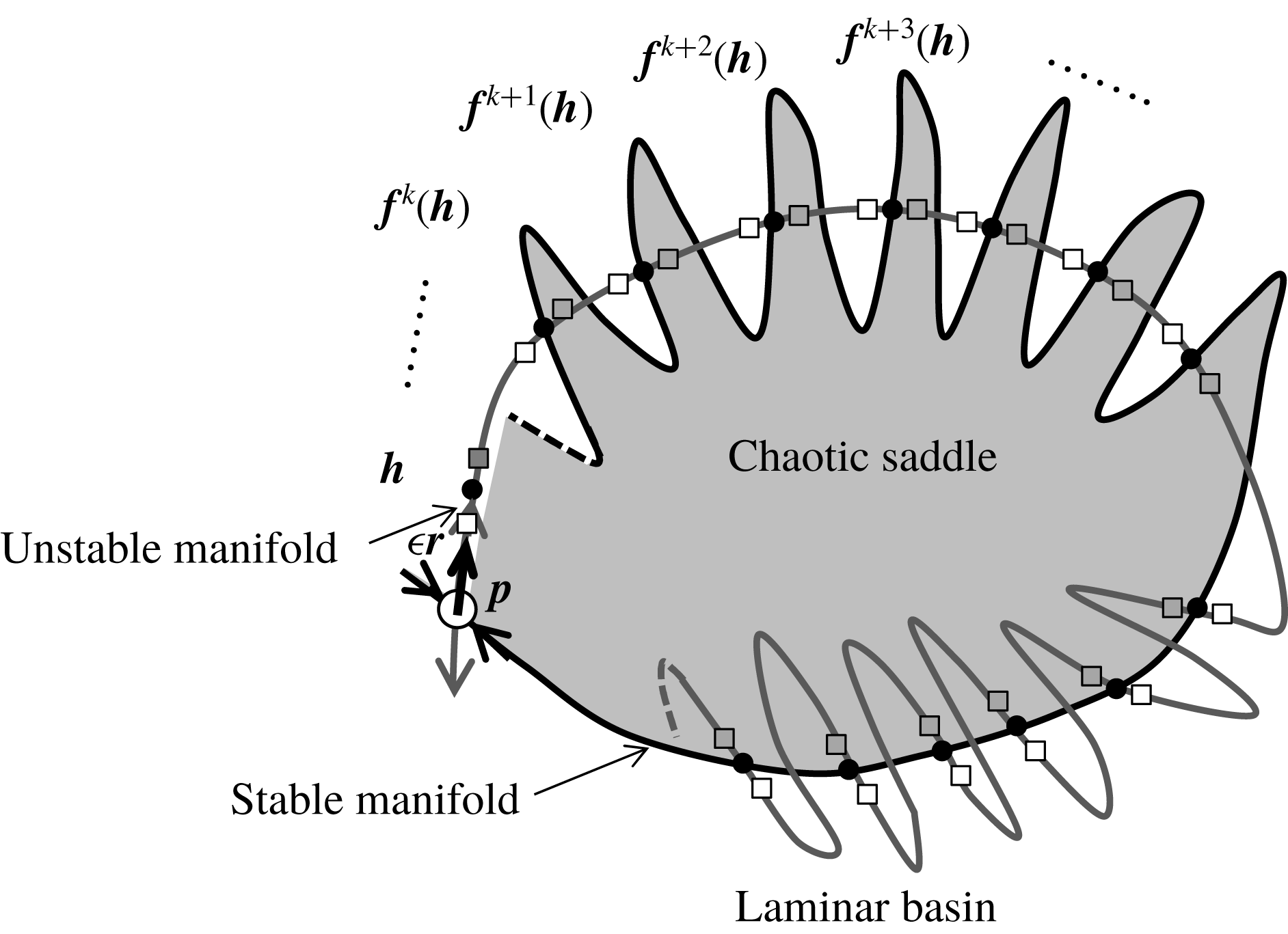
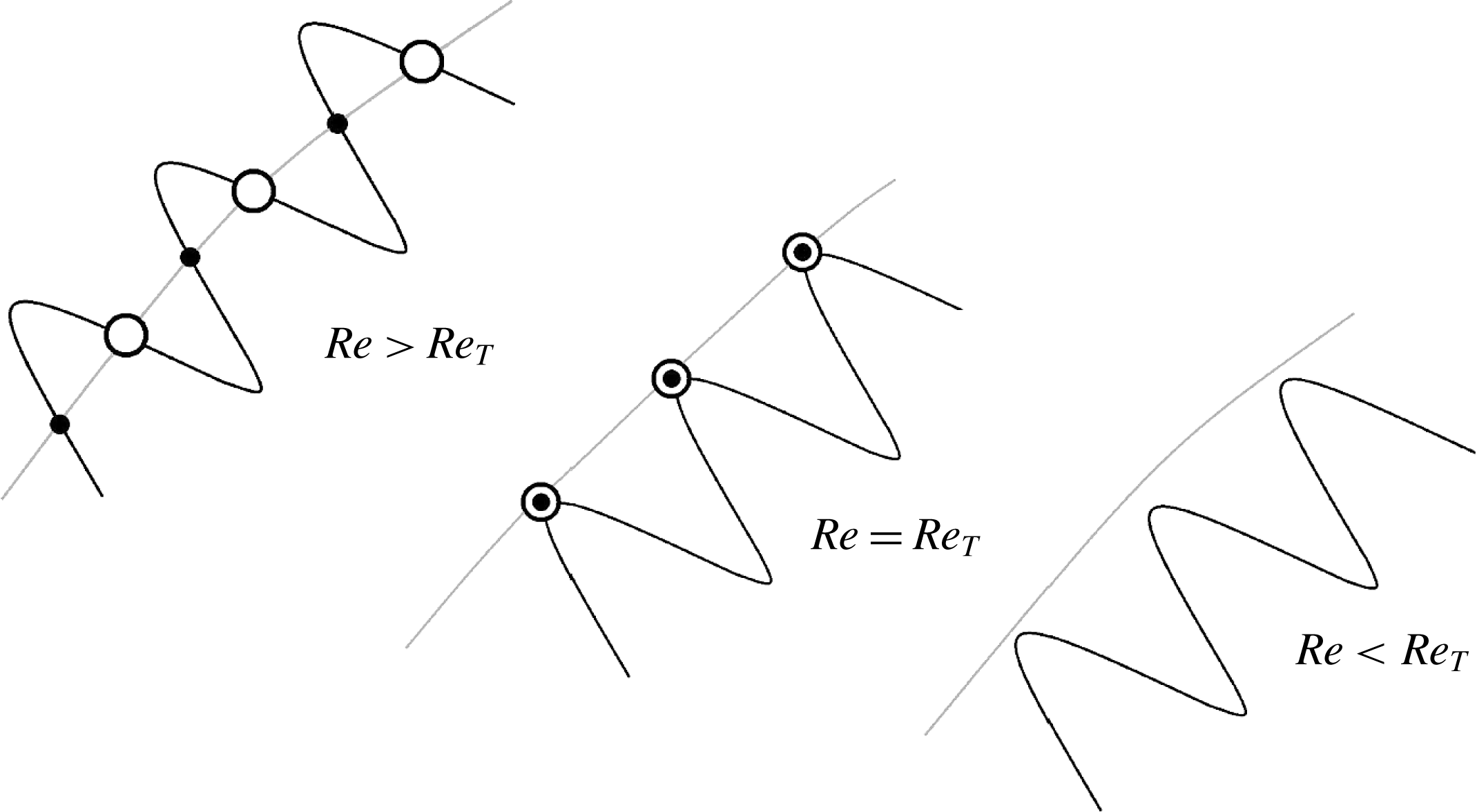
(van Veen & Kawahara Reference van Veen and Kawahara2011). These homoclinic orbits are sets of points that converge to the GPO both forward and backward in time. Such presence of homoclinic orbits to the GPO suggests transversal intersections of unstable and stable manifolds (see figure 1), which then implies the existence of a Smale horseshoe generating chaos (Guckenheimer & Holmes Reference Guckenheimer and Holmes1983; Palis & Takens Reference Palis and Takens1993; Ott Reference Ott2002). Thus, we would like to stress that the computation of orbits homoclinic to the GPO in this study provides a connection between the theoretical determination of transient turbulence and a classical result from chaos theory. Here, we explore the first appearance of homoclinic orbits at what is called a homoclinic tangency, i.e., tangent homoclinic orbits (see figure 2 for a schematic illustration), at a much smaller Reynolds number and show that this tangency marks the onset of transient turbulence that eventually relaminarises.
The unstable and stable manifolds of the GPO and the homoclinic points
 $\boldsymbol{h}$
and
 $\boldsymbol{f}^{n}(\boldsymbol{h})$
(
 $n=1,2,\ldots$
) on the Poincaré section
 $\unicode[STIX]{x1D6F4}$
. The Poincaré section has an intersection at
 $\boldsymbol{p}$
with the GPO. The boundary of the shaded chaotic basin is formed by the GPO and its stable manifold. A homoclinic point
 $\boldsymbol{h}$
is supposed to be close to
 $\boldsymbol{p}$
. The
 $n$
th iterate of the Poincaré map is denoted by
 $\boldsymbol{f}^{n}$
. The unstable and stable manifolds are shown, respectively, by the grey and black curves, and the homoclinic points are represented by black dots. The unstable eigenvector
 $\boldsymbol{r}$
is tangent to the unstable manifold of the GPO at
 $\boldsymbol{p}$
. The squares stand for the sequence of mapped points
 $\boldsymbol{f}^{n}(\,\boldsymbol{p}+\unicode[STIX]{x1D716}\boldsymbol{r})$
(
 $n=1,2,\ldots$
), where
 $\unicode[STIX]{x1D716}$
is a positive small parameter. For the case of
 $\unicode[STIX]{x1D716}$
just below (or above)
 $\Vert \boldsymbol{h}-\boldsymbol{p}\Vert /\Vert \boldsymbol{r}\Vert$
the mapped points are represented by white (or grey) symbols.
Schematic illustration of homoclinic tangency in the Poincaré section. Grey and black lines represent unstable and stable manifolds of the GPO, respectively. Open and closed circles represent two distinct series of homoclinic points, i.e., intersections of two distinct homoclinic orbits. For
 $Re>Re_{T}$
, transversal homoclinic points appear on the transversal intersections of unstable and stable manifolds of the GPO. At
 $Re=Re_{T}$
, homoclinic points start to appear due to tangency of unstable and stable manifolds of the GPO. For
 $Re<Re_{T}$
, homoclinic points do not exist because there is no intersection of unstable and stable manifolds of the GPO.
For identifying the tangency, we use a method inspired by the work of Itano & Toh (Reference Itano and Toh2001), which is related to the edge-tracking algorithm described by Skufca et al. (Reference Skufca, Yorke and Eckhardt2006) and Schneider et al. (Reference Schneider, Gibson, Lagha, De Lillo and Eckhardt2008). This method relies on the fact that the GPO has only a single unstable direction, so that homoclinic points in its unstable manifold can be selected by tuning a single parameter. In the more general case of multiple unstable directions, a more computationally demanding boundary value problem, which includes the adjoint linear equations, must be solved (Doedel et al. Reference Doedel, Kooi, van Voorn and Kuznetsov2009).
In this study, we provide a theoretical description of the onset of transient turbulence in minimal plane Couette flow through the identification of the first homoclinic tangency to the edge state GPO. In incompressible Keplerian shear flow, Riols et al. (Reference Riols, Rincon, Cossu, Lesur, Longaretti, Ogilvie and Herault2013) have reported the possible role of homoclinic and heteroclinic tangles in their numerical experiments leading to chaotic dynamics, but to the authors’ knowledge, the onset of such transient turbulence has yet to be described theoretically. We numerically compute homoclinic orbits to the GPO and track them down with decreasing Reynolds number to identify their onset as tangency. The search leads to a few pairs of distinct homoclinic orbits in which the two homoclinic orbits move closer to each other as the Reynolds number decreases, and eventually collide and disappear at a tangency Reynolds number (see figure 2). Grebogi, Ott & Yorke (Reference Grebogi, Ott and Yorke1983) first identified homoclinic tangency in the Hénon map as a mechanism that causes boundary crisis, i.e., the sudden disappearance of a sustaining chaotic set as it touches a periodic edge state at the critical parameter. In this work we also confirm the relevance of the theoretical determination of the onset Reynolds number of transient turbulence to the numerically observed boundary crisis Reynolds number.
2 Flow configuration and numerical computations
We consider plane Couette flow, i.e., the viscous flow between two moving parallel plates which have a no-slip and impermeable surface and are separated by a distance
 $2h$
. Let
 $x$
,
 $y$
and
 $z$
denote the streamwise, the wall-normal and the spanwise coordinates, respectively, and let their origin be on the midplane. The upper (or lower) plate at
 $y/h=+1$
(or
 $-1$
) moves in the positive (or negative)
 $x$
-direction at a constant speed
 $U$
. The Reynolds number is defined as
 $Re=Uh/\unicode[STIX]{x1D708}$
, where
 $\unicode[STIX]{x1D708}$
is the kinematic viscosity of fluid. Spatial periodicity is imposed on the flow in the
 $x$
- and
 $z$
-directions. The streamwise and spanwise periods are set to the minimal dimensions
 $(L_{x}/h,L_{z}/h)=(1.755\unicode[STIX]{x03C0},1.2\unicode[STIX]{x03C0})$
for sustaining turbulence (Kawahara & Kida Reference Kawahara and Kida2001), i.e., the minimal flow unit first introduced by Jiménez & Moin (Reference Jiménez and Moin1991) and Hamilton, Kim & Waleffe (Reference Hamilton, Kim and Waleffe1995). Although plane Couette flow in a larger periodic domain is closer to real flow in an experiment or to ideal flow in a theory, such an extended system is far beyond a dynamical systems approach to be taken in this paper. Therefore, as the first step to understanding the onset of transient turbulence, we investigate the minimal flow to characterise its onset in terms of a dynamical systems theory. Note that in the minimal flow unit, the Nagata (Reference Nagata1990) steady solution, i.e., an edge state, does not exist, at least at a low Reynolds number (see Jiménez et al.
Reference Jiménez, Kawahara, Simens, Nagata and Shiba2005). Instead, the edge state in this flow is a time-periodic variation, which shows weak, meandering streamwise streaks (Kawahara & Kida Reference Kawahara and Kida2001; Kawahara Reference Kawahara2005). This GPO has a single unstable Floquet multiplier and thus its unstable manifold is two-dimensional and its stable manifold has codimension one in phase space (Kawahara Reference Kawahara2005). Both the GPO and its unstable manifold are contained in a subspace invariant under the spatial symmetries given by reflection in the midplane, followed by a streamwise shift over
 $L_{x}/2$
, and reflection in the streamwise and spanwise directions, followed by a spanwise shift over
 $L_{z}/2$
(Kawahara & Kida Reference Kawahara and Kida2001).
The incompressible Navier–Stokes equation is numerically solved by using a spectral method. The scheme for the numerical solution is essentially the same as that used by Kim, Moin & Moser (Reference Kim, Moin and Moser1987), i.e., Crank–Nicolson for the viscous terms and Adams–Bashforth for the nonlinear terms. The streamwise volume flux and the spanwise mean pressure gradient are respectively set to zero. Dealiased Fourier expansions are employed in the
 $x$
- and
 $z$
-directions, and Chebyshev-polynomial expansion in the
 $y$
-direction. In the representation of a GPO and an eigensolution thereof in phase space, modified Chebyshev polynomials are used instead of the original Chebyshev polynomial to satisfy boundary conditions on the walls (see McFadden, Murray & Boisvert Reference McFadden, Murray and Boisvert1990). Numerical computations are carried out on 33 792 (
 $=\,32\times 33\times 32$
in
 $x$
,
 $y$
and
 $z$
) grid points for the Reynolds number
 $Re\leqslant 520$
. It is confirmed that the behaviour of the numerical solution is qualitatively the same as that for the lower resolution (
 $16\times 33\times 16$
).
We compute the GPO using the Newton–GMRES (generalised minimal residual) method and examine stability of the computed GPO to infinitesimal disturbances with the same periodicities by using the Arnoldi iteration. These numerical procedures employ the above-mentioned time-stepping computation, and are basically the same as that proposed by Sánchez et al. (Reference Sánchez, Net, García-Archilla and Simó2004) and Viswanath (Reference Viswanath2007). In the Newton–GMRES computation a GPO and its period
 $T$
are numerically obtained for a fixed phase of the periodic orbit. The eigenvalues (Floquet multipliers) and the corresponding eigenvectors of the monodromy matrix with respect to the GPO are then computed numerically.
Homoclinic orbits are tracked down by use of ordinary time-marching of an initial point for
 $Re\leqslant 260$
. Take note that the arclength continuation method (van Veen, Kawahara & Matsumura Reference van Veen, Kawahara and Matsumura2011) which was used by van Veen & Kawahara (Reference van Veen and Kawahara2011) to extract homoclinic orbits at
 $Re=400$
is not used at much lower
 $Re$
in this study. Instead, a bisection method, which is similar to the one used by Itano & Toh (Reference Itano and Toh2001), Skufca et al. (Reference Skufca, Yorke and Eckhardt2006) and Schneider et al. (Reference Schneider, Gibson, Lagha, De Lillo and Eckhardt2008) for simple invariant solutions, is used for the numerical computation of a homoclinic orbit. Let us introduce the Poincaré section
 $\unicode[STIX]{x1D6F4}$
such that it can have an intersection at
 $\boldsymbol{p}$
with the GPO and the (only one) unstable eigenvector
 $\boldsymbol{r}$
of the Poincaré map can be on it, as shown schematically in figure 1. We anticipate that on the Poincaré section there are transversal intersections, i.e., transversal homoclinic points, between the unstable and the stable manifolds of the GPO at
 $\boldsymbol{p}$
. We suppose that one homoclinic point
 $\boldsymbol{h}$
is close to
 $\boldsymbol{p}$
. The
 $n$
th iterate of Poincaré mapping of
 $\boldsymbol{h}$
yields other homoclinic points
 $\boldsymbol{f}^{n}(\boldsymbol{h})$
(
 $n=1,2,\ldots$
). Let us now consider the initial point on the one-dimensional unstable eigensubspace, which is approximated by
 $\boldsymbol{p}+\unicode[STIX]{x1D716}\boldsymbol{r}$
for a positive small parameter
 $\unicode[STIX]{x1D716}$
that is to be determined. This initial point is fed to the time-marching code for the numerical computation of homoclinic orbits. If
 $\unicode[STIX]{x1D716}$
is taken to be
 $\Vert \boldsymbol{h}-\boldsymbol{p}\Vert /\Vert \boldsymbol{r}\Vert$
such that
 $\boldsymbol{p}+\unicode[STIX]{x1D716}\boldsymbol{r}=\boldsymbol{h}$
, this initial point is mapped in time on the sequence of homoclinic points
 $\boldsymbol{f}^{n}(\boldsymbol{h})$
(
 $n=1,2,\ldots$
). If
 $\unicode[STIX]{x1D716}$
is just below or above
 $\Vert \boldsymbol{h}-\boldsymbol{p}\Vert /\Vert \boldsymbol{r}\Vert$
, the mapped points deviate from the corresponding homoclinic points along the unstable manifold, as shown in figure 1. An example of the bisection leading to one homoclinic orbit is shown in figure 3 for
 $Re=260$
, which is not far from the first tangency to be discussed later. In this figure the normalised energy input rate per unit time,
 $$\begin{eqnarray}I\equiv \frac{1}{2L_{x}L_{z}(U/h)}\int _{0}^{L_{x}}\int _{0}^{L_{z}}\left(\left.\frac{\unicode[STIX]{x2202}u}{\unicode[STIX]{x2202}y}\right|_{y=-h}+\left.\frac{\unicode[STIX]{x2202}u}{\unicode[STIX]{x2202}y}\right|_{y=+h}\right)\text{d}x\,\text{d}z,\end{eqnarray}$$
is depicted as a function of dimensionless time
 $tU/h$
, where
 $u$
is the streamwise component of the velocity.
 $I$
is also regarded as the normalised wall shear rate, and it takes a value of unity in a laminar state. In the case of
 $\unicode[STIX]{x1D716}$
just below
 $\Vert \boldsymbol{h}-\boldsymbol{p}\Vert /\Vert \boldsymbol{r}\Vert$
, the mapped points are in the laminar basin instead of being on the stable manifold, i.e., the edge of chaos, so that the state point will approach the laminar flow as time goes on (dotted curve in figure 3). On the other hand, in the case of
 $\unicode[STIX]{x1D716}$
just above
 $\Vert \boldsymbol{h}-\boldsymbol{p}\Vert /\Vert \boldsymbol{r}\Vert$
, the mapped points will exhibit (transiently) chaotic behaviour (dashed curve in figure 3). This critically different consequence is a key indicator for one-dimensional bisection as method in searching for a homoclinic orbit with respect to a GPO between laminarisation and transient turbulence. We run a number of initial conditions for different values of
 $\unicode[STIX]{x1D716}$
and look for pairs of
 $\unicode[STIX]{x1D716}$
that are very close to each other where one goes to laminarisation and the other goes to transient turbulence (dotted and dashed curves, respectively, in figure 3). We expect the
 $\unicode[STIX]{x1D716}$
that leads to homoclinic orbit should be in between such pairs since the homoclinic trajectory goes back to the GPO as in the work by van Veen & Kawahara (Reference van Veen and Kawahara2011). We use bisection repeatedly on these pairs of
 $\unicode[STIX]{x1D716}$
to extract a homoclinic orbit with at least three cycles long of almost-periodic oscillations at the end of the orbit (solid curve in figure 3).
The energy input rate
 $I$
of the three different orbits in the course of bisection as a function of time
 $tU/h$
at
 $Re=260$
. Different lines denote initial conditions of different values of
 $\unicode[STIX]{x1D716}$
. The solid curve represents a homoclinic orbit, the early and late stages of which exhibit almost-periodic motion. The dotted and dashed curves eventually deviate from the homoclinic orbit to approach a laminar and transiently chaotic state, respectively.

3 Periodic edge states and bifurcation structure
Figure 4 displays a bifurcation diagram of the minimal plane Couette flow showing a value of the local maximum in a time series of
 $I$
as a function of the
 $Re$
. This bifurcation diagram closely resembles the one reported by Shimizu et al. (Reference Shimizu, Kawahara, Lustro and van Veen2014) for a different physical quantity. The periodic orbit referred to as P1 appears from a saddle-node bifurcation at
 $Re\approx 236.1$
. The lower branch of P1, which is closer to a laminar state for
 $I=1$
than the upper branch, is the GPO and is always linearly unstable. Meanwhile, the upper branch is stable to infinitesimal disturbances with the same periodicities as the periodic orbit in the range of
 $236.1<Re<246.2$
. In this range, however, the upper branch might become unstable to subharmonic disturbances for a longer streamwise or spanwise period. It is confirmed that the lower branch has only one real unstable eigenvalue (Floquet multiplier) for the Reynolds number
 $236.1<Re\leqslant 520$
, as already observed at
 $Re=400$
(Kawahara Reference Kawahara2005). This implies that in this range of
 $Re$
the GPO is always an edge state in the minimal flow unit. The upper branch is found to exhibit an oscillatory instability for
 $Re>246.2$
. A complex conjugate pair of the marginal eigenvalues
 $\exp (\pm \text{i}\,\unicode[STIX]{x1D703})$
at
 $Re\approx 246.2$
has an argument of
 $\unicode[STIX]{x1D703}\approx 1.85$
. Therefore, a torus turns out to arise from this non-resonant bifurcation on the upper branch at
 $Re\approx 246.2$
.
The local maximum
 $I_{max}$
in a time series of energy input at each Reynolds number
 $Re$
. The right figure shows the magnification of the P2 solution branches and subsequent chaos. The lower (or upper) branch of P1 is coloured red (or blue). The lower branch of P2 (or upper branch of P2 and subsequent period-doubling cascade) is coloured green (or black). The chaotic saddle after the first boundary crisis at
 $Re=Re_{cr1}$
is coloured violet. In both figures, stable solution branches are represented by solid lines while unstable solution branches are represented by dashed lines. Vertical grey short dashed lines in (b) denote the critical Reynolds numbers for the two boundary crises at
 $Re_{cr1}\approx 240.46$
and
 $Re_{cr2}\approx 240.88$
. At
 $Re=Re_{cr1}$
, the chaotic attractor (black) touches the lower branch of P2 (green). At
 $Re=Re_{cr2}$
, the chaotic saddle (violet) touches the lower branch of P1 (red), i.e., the GPO. It is important to note that these two boundary crises are related to the homoclinic tangencies at the same
 $Re$
.

Another periodic orbit referred to as P2 also appears from a saddle-node bifurcation at
 $Re\approx 239.8$
. This orbit (whose
 $I$
has four local maxima in time) has an unstable lower branch (which is another edge state) and an upper branch that is initially stable. The upper branch of P2 undergoes period-doubling cascade which leads to a chaotic attractor. A boundary crisis between the chaotic attractor and the upper branch of P1 occurs at
 $Re=Re_{cr1}\approx 240.46$
, as observed in an edge state for a laminar basin by Kreilos & Eckhardt (Reference Kreilos and Eckhardt2012) in symmetric plane Couette flow and by Avila et al. (Reference Avila, Mellibovsky, Roland and Hof2013) in symmetric pipe flow. At this value of
 $Re$
, the chaotic attractor can touch the lower branch of P2 (see the approaches of the black dots to the green dashed curves in figure 4). As a result, points on the chaotic set can ‘leak’ to the stable upper branch of P1. The resulting transiently chaotic set is sometimes called a leaky basin. At the Reynolds number above
 $Re_{cr1}$
, the chaotic attractor is converted to a chaotic saddle and all of the trajectories near it are attracted to the upper branch of P1. Another boundary crisis occurs at
 $Re=Re_{cr2}\approx 240.88$
(see the approach of the violet dots to the red dashed curve in figure 4). At this value of the Reynolds number the chaotic saddle touches the GPO. This second crisis creates a leak for state points eventually going to the laminar attractor. Shimizu et al. (Reference Shimizu, Kawahara, Lustro and van Veen2014) reported that this chaotic saddle forms a fractal basin boundary between the laminar attractor and P1 (upper branch). The numerically observed formation of the latter leaky basin suggests the first homoclinic tangency to the GPO which can lead to transient turbulence eventually relaminarising and thus will be discussed in the next section.
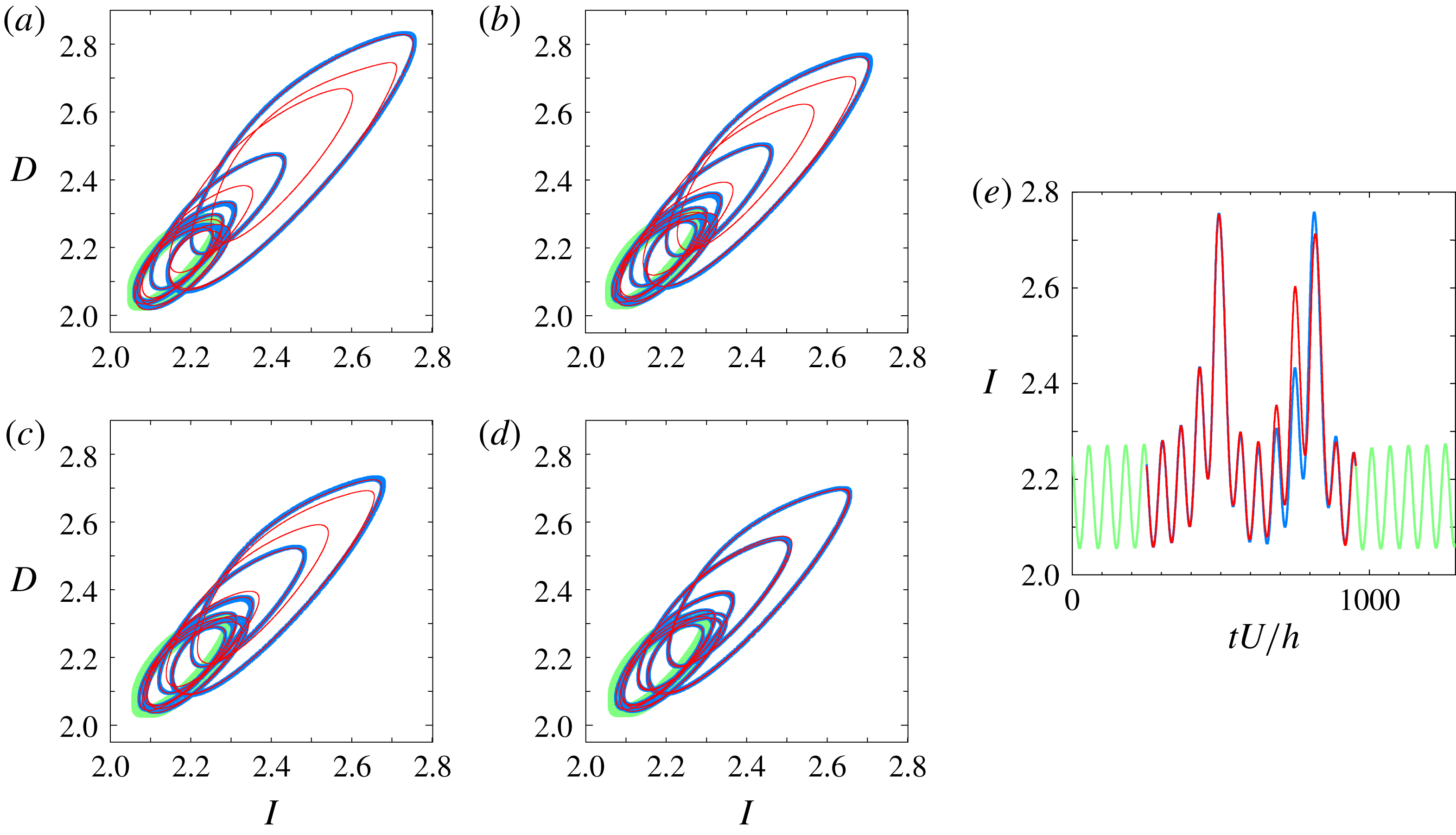
A pair of distinct homoclinic orbits to the GPO that exhibit tangency in the
 $(I,D)$
-projection. The light green line represents the GPO. The blue and red lines correspond to the families of homoclinic orbits referred to as
 $A$
and
 $B$
, respectively. Starting from (a) the pair move closer to each other with decreasing Reynolds number until they merge to tangency at (d). The values of Reynolds number from (a) to (d) are: (a)
 $Re=245$
, (b)
 $Re=242.5$
, (c)
 $Re=241.4$
and (d)
 $Re\approx 240.88$
. The
 $I$
of the two orbits as a function of time at
 $Re=245$
is shown in (e). The blue line is slightly thicker than the red line in order to differentiate one homoclinic orbit from the other, especially during the tangency. A thicker light green line is used to differentiate the GPO from the homoclinic orbits.
4 Onset of transient turbulence as homoclinic tangency
The same as figure 5 but for the
 $(\unicode[STIX]{x1D6FA}_{y}/D,D)$
-projection.

In this section we present the discovered orbits homoclinic to the GPO. We search for homoclinic orbits at
 $Re=260$
using the method described in § 2 and then track them to the lower Reynolds number. Two-dimensional visualisation of homoclinic orbits is used for simplicity’s sake. We encounter several distinct homoclinic orbits during the search and for
 $Re\leqslant 245$
we confirm the presence of a few pairs in which the two homoclinic orbits move closer to each other with decreasing Reynolds number until they eventually disappear. Figure 5 shows the projection of the two orbits, which have been observed to exist down to the lowest (tangency) Reynolds number, onto a two-dimensional plane of normalised energy input rate
 $I$
and normalised energy dissipation rate per unit time,
 $$\begin{eqnarray}D\equiv \frac{1}{2L_{x}L_{z}(U^{2}/h)}\int _{0}^{L_{x}}\int _{-h}^{+h}\int _{0}^{L_{z}}|\unicode[STIX]{x1D74E}|^{2}\,\text{d}x\,\text{d}y\,\text{d}z,\end{eqnarray}$$
 $\unicode[STIX]{x1D74E}$
being the vorticity vector. Similar to that of
 $I$
, the value of
 $D$
in a laminar state is unity. The homoclinic orbits and their tangency are confirmed by projecting them onto another plane,
 $(\unicode[STIX]{x1D6FA}_{y}/D,D)$
, as in figure 6. Here
 $\unicode[STIX]{x1D6FA}_{y}$
is given as
 $$\begin{eqnarray}\unicode[STIX]{x1D6FA}_{y}\equiv \frac{1}{2L_{x}L_{z}(U^{2}/h)}\int _{0}^{L_{x}}\int _{-h}^{+h}\int _{0}^{L_{z}}{\unicode[STIX]{x1D714}_{y}}^{2}\,\text{d}x\,\text{d}y\,\text{d}z,\end{eqnarray}$$
where
 $\unicode[STIX]{x1D714}_{y}$
is the wall-normal component of the vorticity. As seen in figures 5 and 6, even at the highest Reynolds number
 $Re=245$
the former of the two large-amplitude oscillations (i.e., escape out of the light green GPO) are almost consistent between the two homoclinic orbits while the latter are significantly distinct (see figures 5
e and 6
e). As
 $Re$
is decreased these two homoclinic orbits get closer to each other and eventually merge to disappear in tangency at
 $Re=Re_{T}\approx 240.88$
. Such merging and subsequent disappearance of the homoclinic orbits suggest the presence of homoclinic tangency, i.e., the origin of a pair of homoclinic orbits, where below the tangency Reynolds number these two orbits cannot exist (see figure 2). The tangency is verified quantitatively by computing the difference of
 $I$
and
 $D$
in the close vicinity of
 $Re=Re_{T}$
such as
 $$\begin{eqnarray}d_{I}=\sqrt{\frac{\displaystyle \int _{0}^{T}[I_{A}(t+\unicode[STIX]{x1D70F})-I_{B}(t)]^{2}\,\text{d}t}{\displaystyle \int _{0}^{T}[I_{A}(t)]^{2}\,\text{d}t}},\quad d_{D}=\sqrt{\frac{\displaystyle \int _{0}^{T}[D_{A}(t+\unicode[STIX]{x1D70F})-D_{B}(t)]^{2}\,\text{d}t}{\displaystyle \int _{0}^{T}[D_{A}(t)]^{2}\,\text{d}t}},\end{eqnarray}$$
where the subscripts
 $A$
and
 $B$
correspond to the pair of homoclinic orbits and
 $\unicode[STIX]{x1D70F}$
denotes the time period shift optimised so that
 $d_{I}$
or
 $d_{D}$
may be minimal at each
 $Re$
. Least squares fitting is performed using the equation
 $d=K(Re-Re_{T})^{\unicode[STIX]{x1D6FC}}$
, where
 $K$
and
 $\unicode[STIX]{x1D6FC}$
are constants (see figure 7). For both the differences the tangency Reynolds number has been determined as
 $Re_{T}\approx 240.88$
, and the constant
 $\unicode[STIX]{x1D6FC}$
takes a value almost equal to
 $1/2$
, confirming the multiplicity of the two solutions.
Log–log plot of the difference in (a)
 $I$
and (b)
 $D$
between the two homoclinic orbits to the GPO as a function of the increment of the Reynolds number. The lines represent least squares fitting by the function
 $d=K(Re-Re_{T})^{\unicode[STIX]{x1D6FC}}$
in the close vicinity of the tangency Reynolds number
 $Re_{T}$
.
 $Re_{T}\approx 240.88$
and
 $\unicode[STIX]{x1D6FC}\approx 0.50$
in both fittings, while
 $K$
takes a value of 0.011 and 0.013 for (a) and (b), respectively.

No homoclinic orbits to the GPO have been found below the first tangency Reynolds number
 $Re_{T}$
. Dynamical systems theory tells us that the presence of transversal homoclinic orbits (and so transversal homoclinic points on Poincaré section) implies the existence of a Smale horseshoe. The classical Smale–Birkhoff theorem states that transversal crossings of the stable and unstable manifolds in such a Smale horseshoe lead to an intricate tangle of the two manifolds, forming chaotic trajectories in the process (Guckenheimer & Holmes Reference Guckenheimer and Holmes1983; Palis & Takens Reference Palis and Takens1993; Ott Reference Ott2002). The transient chaos eventually relaminarising seen in the previous section is observed just above this first homoclinic tangency. Hence, the onset of transient turbulence eventually relaminarising in this system can be explained theoretically in terms of the creation of chaotic orbits as a consequence of this first homoclinic tangency with respect to the GPO for the laminar flow.
5 Relevance of homoclinic tangency to boundary crisis
(a) The difference
 $d_{I}$
of the lower branch of P2 from a segment on the chaotic attractor which come closest to the lower branch of P2 just before the first boundary crisis. (b) The difference
 $d_{I}$
of the GPO from a segment on the chaotic saddle which come closest to the GPO just before the second boundary crisis. Dashed lines represent the corresponding tangency Reynolds numbers.

It is important to emphasise that
 $Re_{T}=Re_{cr2}\approx 240.88$
, such that the first homoclinic tangency creates the boundary crisis between the upper branch of P1 and the laminar attractor, leading to relaminarisation. Such crisis, which is due to tangency of stable and unstable manifolds, has been demonstrated by Grebogi et al. (Reference Grebogi, Ott and Yorke1983) in the Hénon map. The observed boundary crisis at lower
 $Re$
,
 $Re_{cr1}\approx 240.46$
, between the upper branch of P1 and the chaotic attractor also implies the existence of homoclinic orbits and their tangency with respect to the lower branch of P2. In reality the first homoclinic tangency with respect to the lower branch of P2 has also been confirmed at
 $Re\approx 240.46$
(figure not shown), which is consistent with the crisis Reynolds number
 $Re_{cr1}$
. We can say that as with the second boundary crisis at
 $Re_{cr2}\approx 240.88$
, the first boundary crisis at
 $Re_{cr1}\approx 240.46$
is due to the first homoclinic tangency to the lower branch of P2. The approach of the chaotic attractor/saddle to the lower branch of P2/GPO just before the crisis is verified quantitatively by computing
 $d_{I}$
introduced in § 4 for a segment of the same period as the lower branch of P2/GPO on the chaotic attractor/saddle which comes closest to the lower branch of P2/GPO. Figure 8 shows the differences of the chaotic segments from the lower branches as a function of the Reynolds number. Although a small discrepancy is still seen because of finite-time numerical observation, significant decreases in the difference
 $d_{I}$
can be confirmed just below the tangency Reynolds numbers, as shown in the figures.
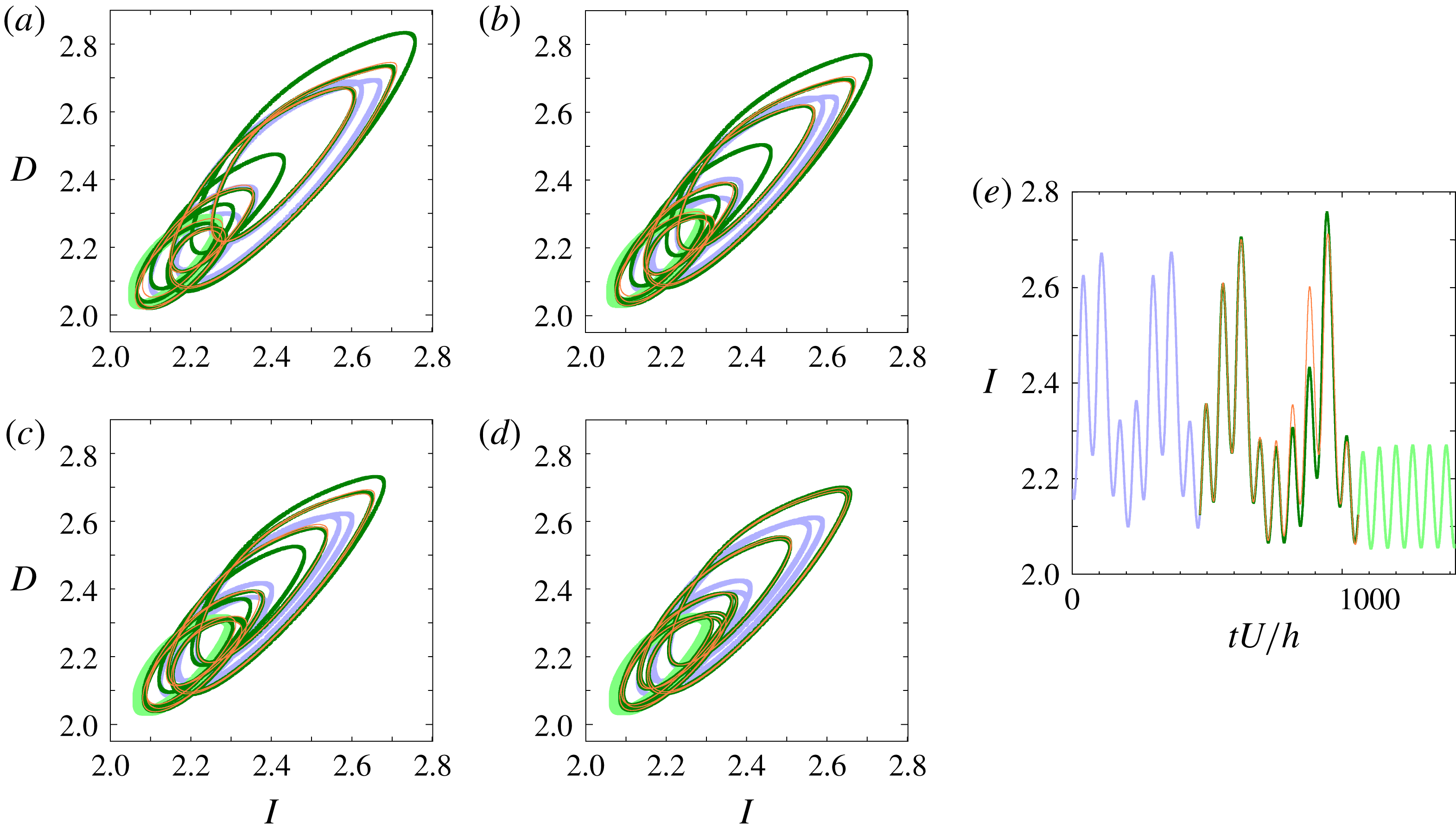
A pair of distinct heteroclinic orbits from the lower branch of P2 to the GPO that exhibit tangency in the
 $(I,D)$
-projection. The light violet and light green lines represent the lower branch of P2 and the GPO, respectively. The green and orange lines correspond to the families of heteroclinic orbits. Starting from (a) the pair move closer to each other with decreasing Reynolds number until they merge to tangency at (d). The values of Reynolds number from (a) to (d) are: (a)
 $Re=245$
, (b)
 $Re=242.5$
, (c)
 $Re=241.4$
and (d)
 $Re\approx 240.89$
. The
 $I$
of the two orbits as a function of time at
 $Re=245$
is shown in (e). The green line is slightly thicker than the orange line in order to differentiate one heteroclinic orbit from the other, especially during the tangency. Thicker light green and light violet lines are used to differentiate the periodic orbits from the heteroclinic orbits.
For homoclinic orbits to the lower branch of P2 another tangency has also been observed at
 $Re\approx 240.56$
. For homoclinic orbits to the GPO two other tangencies have also been found at
 $Re\approx 240.89$
and 241.3. One homoclinic orbit in the pair which has tangency at
 $Re\approx 241.3$
belongs to the family of the homoclinic orbits discovered by van Veen & Kawahara (Reference van Veen and Kawahara2011) while the other belongs to a new family found in this study. The two pairs, one of which has the first tangency at
 $Re=Re_{T}$
and the other of which has the tangency at
 $Re\approx 240.89$
, all belong to new families. Projection onto both the
 $(I,D)$
and
 $(\unicode[STIX]{x1D6FA}_{y}/D,D)$
planes confirms these homoclinic orbits to the lower branch of P2 and GPO as well as their tangency. These homoclinic orbits are paired based on which of them becomes tangent with another one, then the pairs are tracked for increasing Reynolds number. Time evolution of the flow structures along these homoclinic orbits shows a qualitatively similar scenario to the one reported by van Veen & Kawahara (Reference van Veen and Kawahara2011), with the streak becoming less deformed during the bursting event because the homoclinic orbit gets closer to the GPO as the Reynolds number is decreased.
The same as figure 9 but for the
 $(\unicode[STIX]{x1D6FA}_{y}/D,D)$
-projection.
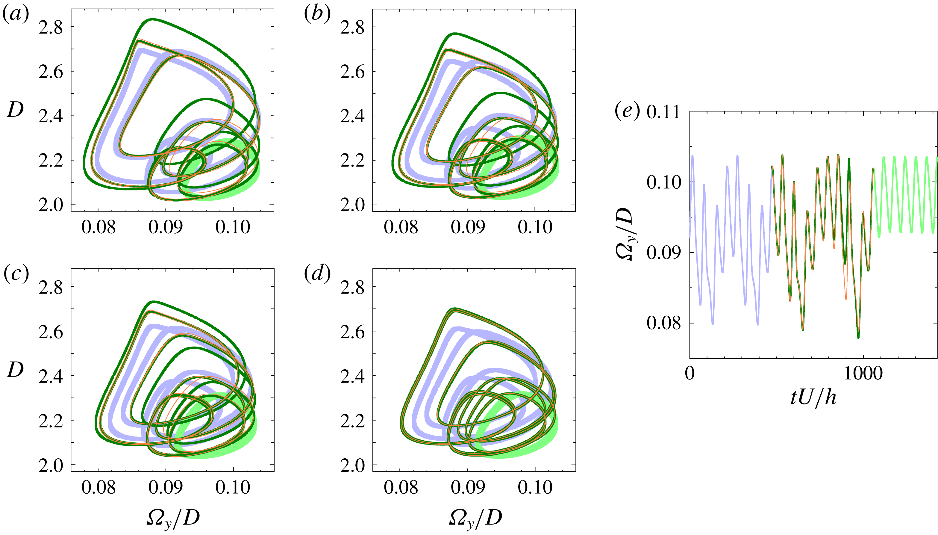
The existence of above-mentioned homoclinic orbits to the GPO and the lower branch of P2 suggests presence of heteroclinic orbits. A pair of heteroclinic orbits from the lower branch of P2 to the GPO has actually been found to arise from the first heteroclinic tangency, i.e., tangent heteroclinic orbits, at
 $Re\approx 240.89$
(see figures 9 and 10).
6 Conclusion
We have reported the homoclinic tangency at
 $Re_{T}\approx 240.88$
with respect to the periodic edge state found by Kawahara & Kida (Reference Kawahara and Kida2001) in minimal plane Couette flow. To our knowledge, the identification of the first homoclinic tangency in this study is the earliest theoretical evidence of a boundary crisis leading to transient turbulence that eventually relaminarises. Although Riols et al. (Reference Riols, Rincon, Cossu, Lesur, Longaretti, Ogilvie and Herault2013) reported the presence of homoclinic tangle at the onset of chaotic dynamics in a Keplerian shear flow, they did not identify the onset as the tangency. We have confirmed that, as with the report by Grebogi et al. (Reference Grebogi, Ott and Yorke1983) on the Hénon map, both the boundary crises at
 $Re_{cr1}\approx 240.46$
and
 $Re_{cr2}\approx 240.88$
are attributed to homoclinic tangencies at the two corresponding critical Reynolds numbers, which is probably the first such result for fluid flow systems. Even though the results here are for a minimal flow unit, the striking similarity of the boundary crisis on the periodic edge state found in this study to that on a streamwise-localised periodic edge state (Avila et al.
Reference Avila, Mellibovsky, Roland and Hof2013) as well as the recent investigation on the unstable manifold of the localised relative period orbit (Budanur & Hof Reference Budanur and Hof2017) in pipe flow encourage us to identify homoclinic tangency in pipe flow, if any, for the theoretical explanation of the onset of spatially localised transient turbulence – that is, a turbulent puff – in experiments.
Acknowledgements
This work has been partially supported by the Grant in Aid for Scientific Research (grant nos. 25249014, 26630055) from Japan Society for the Promotion of Science and the Basic Research Grant from University of the Philippines Los Baños (project code 14828). L.v.V. was supported by an NSERC Discovery Grant. J.R.T.L.’s doctoral study is supported by the Japanese government’s MEXT scholarship (id no. 162100).



