Introduction
The Antarctic continent possesses three types of lakes (e.g. Menzies Reference Menzies1995). Epiglacial lakes are found on the bare ground close to the oceanic boundary of the continent and at nunataks, subglacial lakes are very old water bodies at the base of the ice sheet, and supraglacial lakes form in blue ice regions in the surface layer of the ice sheet in summer. Epiglacial lakes are like normal cold region lakes with a soil or rock bottom, fed by glacial meltwater inflow. They are an important habitat of life in the polar world (Kaup Reference Kaup1994). Subglacial lakes are not yet well known but are very specific physical and microbiological systems at the bottom of the Antarctic ice sheet (e.g. Siegert et al. Reference Siegert, Ellis-Evans, Tranter, Mayer, Petit, Salamatink and Priscu2001). Supraglacial lakes, the topic of the present paper, influence the local heat budget by their increased capacity to absorb solar radiation. These lakes feed liquid water into fractures in the ice sheet, and show sensitivity to climatic conditions and thereby assist detection of regional climate change (e.g. Winther et al. Reference Winther, Elvehøy, Bøggild, Sand and Liston1996). They are extremely low in biota (Keskitalo et al. unpublished data). Supraglacial lakes are a common feature in the Greenland ice sheet, and there they are much more developed and have a major impact on the ice mass balance (Hoffman et al. Reference Hoffman, Catania, Neumann, Andrews and Rumrill2011, Liang et al. Reference Liang, Colgan, Lv, Steffen, Abdalati, Stroeve, Gallaher and Bayou2012). Lake outflows may form moulins into the ice advecting heat into the ice sheet interior and reducing the sliding friction at the base of the ice sheet. Supraglacial lakes also occur in mountain glaciers and there possess potential to create floods in the nearby environment (Bajracharya & Mool Reference Bajracharya and Mool2009).
The depth of supraglacial lakes is of the order of one metre and their surface area is up to several square kilometres. Their thermodynamics is governed by the summer radiation balance: penetration of solar radiation provides heat for subsurface melting of ice, and therefore the surface must be essentially snow-free. A supraglacial lake may have ice cover, if long-wave radiation and turbulent heat losses overcome absorption of solar heat at the surface. In the presence of ice-cover, albedo is fairly low (around 0.4–0.6) due to the bare surface and the thin ice cover over the liquid lake body. Therefore these lakes absorb solar energy about five times more effectively than the snow-covered ice sheet (albedo∼0.9), and so modify the local energy balance. In open surface lakes the albedo is about 0.1 and absorption of solar heat is doubled compared with the bare ice cover lakes. Lakewater masses may also transport latent heat deeper into the ice sheet by convection across the lakewater body and penetration of lakewater into fractures (Chikita et al. Reference Chikita, Jha and Yamada1999, Joughin et al. Reference Joughin, Das, King, Smith, Howat and Moon2008, Hoffman et al. Reference Hoffman, Catania, Neumann, Andrews and Rumrill2011). In fall, supraglacial lakes start to freeze down from the upper surface, as lakes usually do (e.g. Leppäranta Reference Leppäranta2009) and up from the bottom, and in principle it is possible that pockets of liquid water could survive over the winter. Changing of a supraglacial lake from seasonal to perennial would accelerate local melting, lead to lake growth and eventually formation of fractures taking the water in and ending in a major change in the local glacial environment. However, we are not aware of this kind of development in Dronning Maud Land, and in our study region a major climate change would be necessary for perennial lakes to form.
In this paper we examine supraglacial lakes using data from field surveys in two summers in western Dronning Maud Land. The observation programme was carried out in FINNARP (Finnish Antarctic Research Programme) expeditions during the summers 2004–05 and 2010–11. Three lakes at the sides of three separate nunataks were mapped. Ice and snow samples were taken, and one lake was equipped with an automatic radiation station. The final results of these lake investigations are presented, including their cross-sectional and vertical structure, surface radiation balance, and penetration of sunlight into the ice and water. A scaling analysis is performed on the life history and dimensions of supraglacial lakes, validated by the observations.
Measurement campaign
Sites
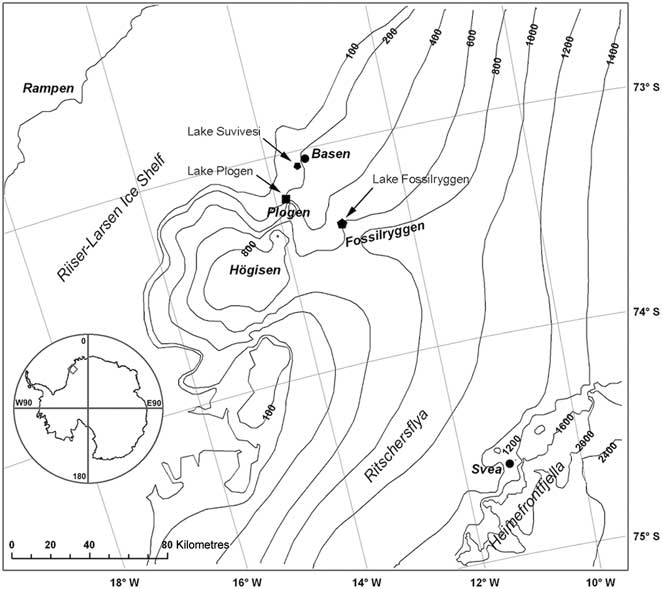
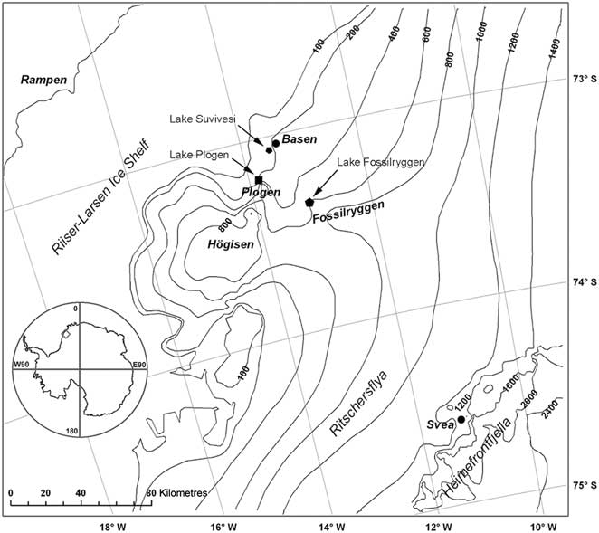
Fieldwork in FINNARP 2004 and 2010 expeditions was carried out in the vicinity of the Finnish Aboa Station during December–January 2004–05 and 2010–11 (Kanto et al. Reference Kanto, Mattila and Leppäranta2007, Järvinen et al. Reference Kanto, Mattila and Leppäranta2012). The station is located on Basen nunatak (unofficial name) at 73°02.5′S, 13°24.4′W, near the grounding line of Riiser-Larsen Ice Shelf in the Weddell Sea, c. 125 km inland from the shelf edge (Fig. 1). The top of Basen is 584 m above sea level and about 380 m above the surface of the neighbouring ice sheet. For investigations of supraglacial lakes, the primary site was lake Suvivesi (unofficial name) at the south-western side of Basen. Two additional reference sites were taken from Plogen and Fossilryggen nunataks (unofficial names) at distances of 25 km and 50 km, respectively, south of Basen (Fig. 1). At Basen and Plogen, the lakes were at the level of the surface of the ice sheet, whereas at Fossilryggen the lake was in a 200-m deep hollow around one of the nunatak peaks, about 400 m above sea level.
A map of western Dronning Maud Land showing the nunataks Basen, Plogen and Fossilryggen, where the study lakes were located. The contours show the elevation above sea level (m).
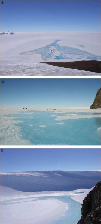
Lake Suvivesi (Fig. 2a) extends 4 km out from Basen and is larger than the other two study lakes. Its maximum surface area is about 7 km2. This area has bare ice surface. The lake forms and grows from patches, and therefore it is difficult to determine the evolution of the surface area. At Basen there were also a few smaller ponds at the base of the mount. Lake Suvivesi was visited regularly for observations and it was equipped with an automatic radiation station. The lake at Plogen (Fig. 2b) was visited once in the first summer and twice in the second summer, and Fossilryggen lake (unofficial name, Fig. 2c) was visited just once, on 31 December 2004. In summer 2003–04 the geochemistry of the same lakes had been examined providing basic geochemical information of the lakes (Lehtinen Reference Lehtinen2006). Lake Suvivesi was also used as a source of household water for Aboa Station, and therefore practical experience of its formation is available since 1990.
Photographs of the lakes at a. Basen, 15 January 2005, b. Plogen, 24 January 2005, and c. Fossilryggen, 31 December 2004. In a. a low moraine ridge is seen in the middle of the lake, and Plogen nunatak shows up on the left, approximately 25 km away.

Data collected
The basic structure of all lakes was mapped by drilling with a Kovacs drill (diameter 55 mm) for the layers of solid ice, water and slush. Cross-sectional profiles of lake Suvivesi were drilled several times to obtain the evolution history. Ice samples were taken with a core drill from the surface down to 1–2 m beneath the lake bottom into the solid ice sheet. The cores provide information about the lake history, crystal structure of ice, and impurities. Ice temperature profiles were determined from the cores at the sites.
The radiation station in lake Suvivesi recorded the net radiation, the spectrally integrated incoming and outgoing solar radiation at the surface, and quantum PAR (photosynthetically active radiation, 400–700 nm) level in the lake. The recording time interval was ten minutes. Net radiation was measured with a Kipp & Zonen NR Lite net radiometer just above the ice surface. The spectral range was 0.2–100 μm. The instrument was mounted on the end of a pole, which was clamped onto a tripod with sensor head about 1 m above the ground. Downwelling and upwelling solar planar irradiances just above the surface were measured with a Middleton EP-16 pyrano-albedometer system (spectral range 0.30–3.0 μm). The instrument is a modified thermopile pyranometer with an additional inverted sensor assembly. The instrument was mounted on a tripod in a similar fashion as the net radiometer, and the two tripods were deployed close to each other.
Quantum PAR level was measured at several depths down to 1 m with MDS-L PAR sensors (Alec Electronics, Japan). The sensors are 115 mm long and 18 mm in diameter, and they are equipped with internal memory (see e.g. Leppäranta et al. Reference Leppäranta, Terzhevik and Shirasawa2010). The sensors were lowered through narrow drill holes into the lake and anchored to the top surface with bamboo crosses. Transforming quantum irradiance (μmol m-2 s-1) to irradiance power Q (W m-2) requires that we know the spectral distribution of light (see Arst Reference Arst2003). For white light, which can be assumed for sunlight at the surface, we have q/Q = 4.60 μmol J-1, but in ice and water the light spectrum changes significantly with depth, influencing the q/Q ratio. Following the work of Reinart et al. (Reference Reinart, Arst, Blanco-Sequeiros and Herlevi1998) for Finnish and Estonian lakes, we use q/Q = 5.0 μmol J-1, which gives an accuracy better than 10%.
Weather data were provided by the FINNARP weather station located on Basen at 497 m altitude, about 300 m above lake Suvivesi (see Kärkäs Reference Kärkäs2004). These data provide incoming and outgoing solar radiation, air temperature and humidity, and wind speed and direction. Cloudiness data were available from regular weather reports sent from Aboa.
Structure of supraglacial lakes
Vertical profile evolution
Lake Suvivesi 2004–05
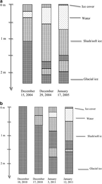
In the summer 2004–05 lake Suvivesi was profiled three times (Fig. 3). The first visit was made on 14 December, when there was already a thin liquid water layer in the lake. The first profile was drilled on the following day. In the central part of the lake, the average thickness of the surface ice was 20 cm and the thickness of the liquid water body was also about 20 cm. Beneath the water body there was a 35–50 cm thick layer of slush or soft ice. In this layer the ice had lost its integrity as the porosity of ice was more than the critical limit of no strength. Porosity, defined as the relative volume of liquid water, is 30–50% at this critical limit.
The vertical profile of lake Suvivesi in a. December 2004–January 2005, and b. December 2010–January 2011.

After this first survey on 14 December, the lake grew vertically and laterally. This means that the porosity of ice continued to increase, and the slush layer expanded. In the central patches of the lake the liquid water content increased up to 100%, starting from the depth of the maximum net energy flux, and spreading upward and downward from there. Thus, it is convenient to define the lake body as the volume where porosity is in the range of 30–100%, i.e. from the limit when ice loses its integrity to full liquid water. In the horizontal direction, growth of the lake involved separated patches of water and slush that expanded and joined together into a more continuous three-dimensional lake body.
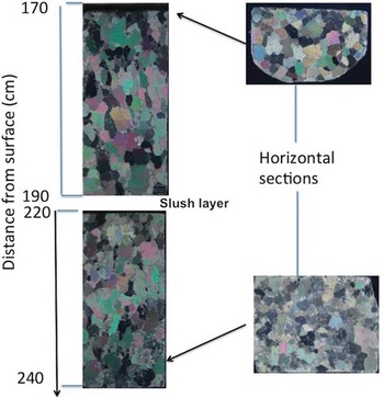
A midsummer profile (29 December 2004) showed 10 cm thick ice cover over a 50 cm thick water body on top of a 65 cm thick slush layer. Beneath the slush there was soft ice down to 150–200 cm from the surface, and then there was hard ice that can be taken as the lake bottom. However, a remarkable feature was that a sediment-rich slush pocket was found at about 20 cm below this lake bottom. On 17 January, the liquid water body was mostly 60–80 cm deep, and the maximum depth was 100 cm. The slush layer below was 70–80 cm thick. The surface ice cover was mostly 5–10 cm thick, and in a few small spots the surface was open. Beneath the water-slush system there was a 20 cm layer of hard ice and then a 25 cm slush layer containing many sediment particles. The crystal structure of the hard ice sheet below the lake bottom showed granular shape and size of 1–3 cm (Fig. 4). At the end of the field season (1 February) there was still much free liquid water available.
Crystal structure of ice below the bottom of lake Suvivesi, summer 2004–05 in the layer 170–240 cm. A slush layer was found in the depth range 190–220 cm. The sample was taken on 29 December 2004.

Spatial sampling and drilling of lake Suvivesi showed that the lake had a patchy structure rather than being a well-defined three-dimensional body. This patchiness came from the variations in the albedo and light attenuation coefficient. In the beginning the lake was a discrete, non-connected set of liquid water and slush pockets, and in the course of time these grew laterally into larger bodies. The bottom of the lake was very uneven, showing deeper hollows caused by sinking stones or sand absorbing solar heat, and water flow spirals penetrating into the ice sheet. These circular hollows were 40–50 cm in diameter. Their water depth exceeded the general level, reaching 150 cm, the ice was soft to more than 3 m depth, and sediment particles were found in this deep soft ice.
Lake Suvivesi 2010–11
In the summer 2010–11, the ‘birth’ of lake Suvivesi took place in the beginning of December. The lake was first visited on 4 December, at which time there was a moist layer at 0°C in the depth range 50–100 cm but no free liquid water. Beneath 1 m depth it was hard ice to 3 m (the maximum depth drilled). Household water could be pumped out of the lake only from 10 December.
The subsequent vertical and lateral evolution of the lake showed similar features as in 2004–05. Starting from patches, the lake deepened and patches expanded and joined together. The top ice layer became thinner with a full liquid water layer below and slush or soft ice underneath (Fig. 3). The deeper part had more variability than in 2004–05. In most cases, one under-lake slush pocket at 150–200 cm depth was found, with hard ice below that layer. In one case there was a double structure, hard ice-slush-hard ice-slush and then hard ice sheet, but all above 200 cm depth. An extreme case was the location of a soft ice layer at 280–310 cm depth; then the surface was smooth, bright blue ice. Sediment particles were found from the under-lake ice sheet, usually in the depth range 150–200 cm but in one case as deep as 350 cm. The sediments consisted of fine-grained soil and gravel. Until the end of the radiation measurements, on 23 January, the total or net daily flux was always positive.
Lakes at Plogen and Fossilryggen
The other study lakes showed similar structure. One sampling site was chosen in each of these lakes in the central region. In 2004–05 the Plogen lake (unofficial name) was visited on 24 January. There was an 11.5 cm surface ice layer and an upper liquid water layer down to 118 cm from the surface. Below that, there was a 25 cm porous ice layer, and a deep slush pocket was found at a depth of 143–151 cm.The next metre (to the lower limit of our drill hole) was hard ice with gravel inclusions at 235 cm depth. Thus the ice structure was quite close to lake Suvivesi in the same summer.
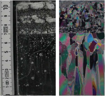
The Plogen lake site was visited twice in 2010–11. On 20 December it was full ice without any moist layers, and therefore the lake was born at least ten days after lake Suvivesi. On 20 January there was mostly a 40 cm surface ice layer, then a 62 cm thick slushy lake body, with hard ice below that. At the outer boundary of the lake there was a narrow zone with a thin surface ice layer, thus, the lake was not as well developed as in 2004–05. The crystal structure beneath the lake bottom was as in lake Suvivesi, however, crystals as large as 5 cm were found. The thin section of the 11.5 cm surface ice layer was prepared showing a thin layer of small crystals (< 1 cm), a thin transition layer and then columnar grains up to 5 cm long (Fig. 5). These results are consistent with observations from seasonally freezing lakes in lower latitudes (e.g. Leppäranta Reference Leppäranta2009).
The structure of the surface ice layer in Plogen lake. Left: thick section in normal light, right: thin section in polarized light. The scale is given on the left (numbers in cm).

The lake in the hollow in Fossilryggen was visited on 31 December 2004. The lake had developed well by that time. The location (Fig. 2c) seemed to be effective in collecting solar radiation and also in protecting the lake from turbulent heat losses. At the primary sampling site the surface ice was 10 cm thick but over large areas the thickness was below 5 cm. The main body of the lake was 98 cm deep, and the lower layer extended to 230 cm with alternating soft and hard layers. The crystal structure of the ice below the lake bottom was similar to lake Suvivesi.
General structure of supraglacial lakes
Based on the two seasons, the summer structure of the central area of lake Suvivesi can be summarized as follows. The lake is seasonal, so that it starts to form in the solid ice sheet in the beginning of December. At about 10 December there is enough liquid water for water supply to Aboa Station (water usage was about 1 m3 per day). The timing has a very small interannual variability. At the initial stage the lake appears patchy in the horizontal plane. In January there is a 0–10 cm thick ice cover on top and the lake body extends down to about 200 cm depth consisting of two layers (Fig. 3). The main, upper layer is mostly liquid water and extends down to the depth of 0.5–1 m. The lower layer is a soft bottom layer and contains slush and hard ice. It contains at least one slush sub-layer and one hard ice sub-layer and the deepest part is an ‘under-lake slush pocket’, at the bottom of which there are gravel and soil sediments. The source of this sediment is most probably the neighbouring nunatak. After the summer warm peak in atmospheric conditions in mid-January, the surface ice layer starts to strengthen but the radiation balance is still positive and the main body of the lake continues to develop. Our data do not go beyond 1 February, and it is not known exactly when the lake shrinking by freezing begins. In the closing period of the lake, the growth of ice is expected to be 1–2 cm per day, based on experience of lake ice growth in general. This means that the lake would be completely frozen by April–May. Thus, the inferred age of the lake is 4–6 months, 1–2 months for growth and 3–4 months for close-up. Observations from Plogen and Fossilryggen show similar evolution but the exact timing depends on the location.
The surface of a supraglacial lake may be liquid water or ice depending on the heat fluxes and surface heat balance. In Greenland there are open water lakes (Liang et al. Reference Liang, Colgan, Lv, Steffen, Abdalati, Stroeve, Gallaher and Bayou2012), but in our study region in western Dronning Maud Land the lakes had ice cover. The surface ice layer exists because the surface heat balance in this region is negative. Much of the incoming solar radiation penetrates into the ice (and liquid water beneath), and the surface absorption does not compensate for the thermal radiation loss. Only in the peak of the summer, a few days in mid-January, melting surfaced in some spots and the ice bearing capacity was below the level needed for on-ice walking or skiing. The thin ice cover corresponds to the ‘cold skin phenomenon’ observed in lower latitude lake and sea surfaces in daytime calm summer conditions (e.g. Fedorov & Ginzburg Reference Fedorov and Ginzburg1992).
The presence of hard and soft sub-layers in the lower layer is most probably due to the variability of the absorption coefficient of solar radiation with depth caused by sediments and ice crystal structure. The absorption coefficient of the sediment-rich ice is much larger than that of the clear ice, and this enables more intensive heating deeper even though the level of radiation is less. Thus in summers sediments have melted their way down. The presence of the concentrated sediment layer below 200 cm reflects the maximum depth of the lake in recent history. The bottom of lake Suvivesi was quite uneven. Superposed on smoother geometry, there were holes due to condensed sediment accumulations, which absorbed sunlight and melted their way deeper.
A seasonal supraglacial lake is a stationary phenomenon. Summer growth of the lake is forced by the solar radiation, which is primarily dependent on cloudiness, while winter freezing is primarily dependent on air temperature. If the liquid water volume becomes large enough, the water pressure may crack the ice sheet and the lakewater would disappear into the interior of the ice sheet, slowly or catastrophically into moulins. This has been observed in the Greenland ice sheet (Joughin et al. Reference Joughin, Das, King, Smith, Howat and Moon2008, Hoffman et al. Reference Hoffman, Catania, Neumann, Andrews and Rumrill2011). It would be valuable to know whether a lake closes up fully in winter. Ice growth in winter would decrease in a warming climate, and after a certain limit the lake would turn perennial. This would further accelerate the long-term growth of the lake. In our drillings, however, no deep-water layer was found in the beginning of summer and we therefore conclude that the present study lakes are still seasonal.
Bog or lake?
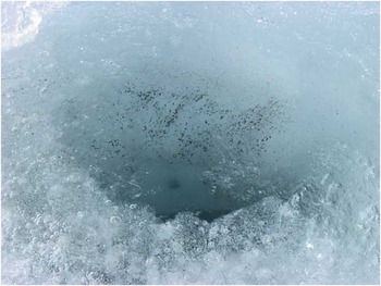
The central area of the three supraglacial lakes had well developed two-layer structure (surface ice on top and a well-defined water body). However, looking toward the boundary area, supraglacial lakes could be regarded as ‘supraglacial bogs’, by analogy with wetland areas. The distribution of the soft and slushy ice layer goes far beyond the boundaries of liquid water body as shown by the light-blue zone encircling lake Suvivesi in Fig. 2a. Also analogous to marshlands, there are small ‘bogholes’ in the light-blue zone, containing slush with no bearing capacity. Their diameter and depth are of the order of one metre. These bogholes form in concentrated patches of sediments, which have come from the neighbouring nunatak (Fig. 6). The sediments were easy to observe and were found in all tested bogholes. How these sediment pockets form is not clear. They could be the result of the bog drainage system.
A boghole showing fine sediments and deeper gravel particles. The diameter of the hole is about 30 cm.

Supraglacial lakes - or bogs - can thus be characterized as water bodies consisting of slush with varying concentration of ice crystals. Take the water body as {ν > ν0} where ν is porosity (relative volume of liquid water) and ν0 is the maximum porosity, which still keeps the integrity of the ice. Beyond the boundary of {ν > ν0} the porosity decreases. By the expansion of the boundary, the ice sheet surface layer turns into ‘bog’ and ‘lake’ as ice loses its integrity. Due to pressure variations, the liquid water in the bog may flow as determined by its hydraulic conductivity and hydraulic potential. To change from ice lattice to slush the liquid water portion should be 30–50%, i.e. ν0 <  $$\[--><$>\frac12<$><!--$$. There are no direct measurement data for this limit but investigations of lake ice melting support this threshold (Jakkila et al. Reference Jakkila, Leppäranta, Kawamura, Shirasawa and Salonen2009). Also, it is known that sea ice strength decreases with brine volume, νb, in proportion to
 $$--><$>\rm exp({\rm{ - }}5.88\sqrt {{{\nu }_{\it b}}} )$$$ (Weeks Reference Weeks1998). At νb = 0.5 the strength is only 1.6% of the strength at νb = 0, and therefore we would expect that ν0 < 0.5. In the middle of summer the core water body of supraglacial lakes becomes ice-free.
In the summer 2010–11, water-pumping experiments were made to examine the hydraulic conductivity of the ‘ice bog’. They were performed in connection with the water take-up for Aboa water supply. Water was pumped into a 1 m3 container of a Nasu vehicle, which weighs seven tons and thus requires the ice to have significant load-bearing capacity. Therefore the water extraction site was in the boundary region of the lake where the surface ice thickness was 15–30 cm with additional support from the underlying slush. Because of the lake evolution the site was changed three times during the field season.
The Dupuit well equation (e.g. Raghunath Reference Raghunath2007) was used to estimate the hydraulic conductivity:
 $$2\pi {{r}_0}DK\frac{{\partial \zeta }}{{\partial r}}\: = \:V,\eqno\rm$$
where r 0 is the radius of the pump hole (7.5 cm), D is the depth of the pump hole (80 cm), K is hydraulic conductivity, ζ is the water surface level at the site, r is the distance from the centre of the hole, and V is the discharge rate in pumping. During the pumping at fixed rate for 10–15 min, a steady state condition was achieved and Eq. (1) can be applied.
The results were as follows:
Site 1. 14–17 December: hydraulic conductivity increased from 0.25 to 0.80 cm s-1; the site was closed because driving there across the lake was no longer possible.
Site 2. 18–27 December: hydraulic conductivity was 1.5–2.0 cm s-1 during the first week but suddenly increased to 8.0 cm s-1 on 27 December.
Site 3. 28 December–27 January: initial hydraulic conductivity was 0.8 cm s-1, increased to 2.0–6.2 cm s-1 from 4–14 January, and from 18–27 January was as high as 20–30 cm s-1; this last period was already late summer, and night-time heat losses had probably strengthened the surface layer ice so that it was possible to use the site to the end.
We also conducted a Darcy-type experiment (e.g. Raghunath Reference Raghunath2007) to estimate the hydraulic conductivity of closely packed slush. A pipe, 1 m long and with a diameter of 20 cm, was filled with slush, tilted, and then water was allowed to flow through. The hydraulic conductivity was obtained from the time water flowed through the pipe, resulting in K = 6.3 cm s-1. This serves as a good reference to the pump tests, denoted by K* below. When K < K*, the ice bog has some integrity but when K > K* the flow channels have opened into the slush and the water flows well. Water storages with hydraulic conductivities K > 0.01 cm s-1 are classified as good in groundwater hydrology, and conductivities K > 1 cm s-1 are typical for gravel. Knowledge of the hydraulic conductivity is necessary for modelling the circulation in supraglacial lakes and it serves also as an index for the internal structure of the lake.
Impurities
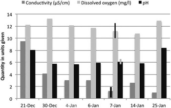
Lake Suvivesi water was very clean, classified as an ultra-oligotrophic lake. The electric conductivity was 1–10 μS cm-1 (referenced to 25°C), dissolved oxygen was 10–12 mg l-1, and pH was 6–8. Conductivity decreased during the summer and pH had a minimum in the middle of the summer (Fig. 7). Similar levels and temporal variations were observed in other monitoring sites as well. A 100 m square area was sampled on 7 January (ten sites), resulting in conductivity 1.26 ± 0.94 μS cm-1, dissolved oxygen 11.2 ± 1.3 mg l-1 and pH 6.1 ± 0.3.
Conductivity (referenced to 25°C), dissolved oxygen and pH in lake Suvivesi, December 2010–January 2011. For 7 January, ± one standard deviations are shown by the narrow columns.

There were no systematic spatial variations of these parameters within the lake. Closer to the nunatak the conductivity and pH were similar as in the central area. In 2010–11 the total nitrogen and phosphorus were 60–100 mg m-3 and 1–2 mg m-3, respectively, close to the levels recorded in the surface snow layer (Keskitalo et al. unpublished data). We conclude that the transport of surface material from the nunatak bare ground to lake Suvivesi was by winds rather than by hydraulic systems.
Ice cores had gravel and soil inclusions, probably originating from the nearby nunatak. The largest pieces were 1–2 cm. They appeared to be widespread, since they were captured in all deeper (more than 2 m) ice cores. In bogholes, fine sediment was usually seen in the bottom and sides (Fig. 6), at times gravel particles were also present. Nunatak sediments were abundant in epiglacial ponds at the foot of the nunataks (Keskitalo et al. unpublished data).
Thermodynamics of supraglacial lakes
Heat budget
The surface heat budget of the ice sheet consists of the radiation balance, turbulent heat fluxes and precipitation. The last one would be important if there were phase changes involved, i.e. liquid precipitation falling on ice. Such cases did not occur during our study periods. In our data the radiation balance was the dominant factor except during heavy storms with intense turbulent heat exchange. In strong southerly wind conditions the latent heat flux can be important since the descending polar air is very dry. In connection with dry katabatic outflows the turbulent heat flux becomes comparable to the radiation balance but such cases are transient and are unimportant for monthly mean fluxes.
Temperature profiling of the water body and the ice cores of the study lakes showed that, in midsummer, the temperature below the water body was from -0.1°C to 0°C down to 3 m depth. In the surface ice cover, lower values (from -2°C to -1°C) were recorded due to the thermal radiation losses. In the lake body, adding heat to liquid water leads to convection and transfer of the heat to melting at the bottom that keeps the water temperature at the freezing point. In the snow-covered ice sheet in the study region, the temperature is about -15°C at 4 m depth in January (Granberg et al. Reference Granberg, Cliche, Mattila, Kanto and Leppäranta2009). The radiational heating is, therefore, very effective in the surface layer of blue ice. The monthly mean air temperature is -5.5°C in January and -21.9°C in August at Aboa weather station (Kärkäs Reference Kärkäs2004).
The incoming solar radiation (Q s0) at the surface of an ice sheet is partly reflected and scattered back and partly absorbed by the underlying medium. The former part is αQ s0, where α is albedo. The absorbed radiation, (1–α)Q s0, is further divided into penetration (proportion γ) and surface absorption (proportion 1 - γ); the partition is fairly stable and γ ≈  $$\[--><$>\frac12<$><!--$$ (optical, ultraviolet and a small fraction of near-infrared solar radiation penetrate the surface layer deeper than 5–10 cm). In the evolution of the lake the component of solar radiation penetrating the surface is a critical quantity. The light level just beneath the surface is denoted as Q* = (1–α)γQ s0 and Q s = Q s(z) is the distribution of light with depth.
Albedo shows a particularly large variability over snow and ice surfaces. Our measurements at lake Suvivesi show that albedo varied within the range 0.4–0.6. The variations were mostly due to snow accumulation and transport during the summer. A thin, patchy snow layer at times appeared on the surface but was then transported away by wind. For a thin lake ice cover, albedo is expected to decrease with ice thickness down to 0.2 for thickness less than 10 cm ice (e.g. Ishikawa et al. Reference Ishikawa, Takizawa, Kawamura, Shirasawa and Leppäranta2003). Our sensors were never on ice this thin for practical reasons. The growth of a supraglacial lake could experience a positive feedback since the decrease of albedo with surface ice thickness would further accelerate the lake growth.
The surface heat balance is expressed as:
 $${{{ {Q}}}_{\rm{0}}}\, {\rm{ = }}\, ({\rm{1 \!\! -\!\alpha }})({\rm{1\!\!-\!\gamma )}}{{{\rm{Q}}}_{{\rm{s0}}}}\, {\rm{ + }}\, {\repsilon}{{{\rm{Q}}}_{{\rm{L}}\downarrow }} \, {\rm{ + }}\, {{{\rm{Q}}}_{{\rm{L}} \uparrow }}\, {\rm{ + }}\, {{{\rm{Q}}}_{\rm{T}}}{\rm{,}}\eqno\rm$$
where ε ≈ 0.97 is the emissivity of ice, Q L↓ and Q L↑ are the atmospheric and surface thermal radiative fluxes, respectively, and Q T is the turbulent heat flux. Net radiation Q s0 and αQ s, were measured in the radiation station. The surface emission can be estimated from the Stefan-Boltzmann law and the known emissivity and, taking γ =  $$\[--><$>\frac12<$><!--$$, the atmospheric thermal radiation is obtained as the residual. If the ice surface is at the melting point, the thermal radiation loss is 306 W m-2. This holds within 5% for temperatures down to -3.5°C. Turbulent fluxes were not continuously measured. Sensible heat flux is low in summer in the study region but, according to our measurements, sublimation can be 1–2 mm water equivalent per day in windy conditions, corresponding to latent heat loss of ∼45 W m-2. However, these losses are transient and mainly reflected in the variations in the thickness of the surface ice layer.
The attenuation of light in ice and water is wavelength-dependent, however, for simplicity here we assume that it is constant across the PAR band. We take the vertical co-ordinate z to be positive downward. Light attenuation is described by a linear law analogous to Beer's absorption law: dQ s/dz = -κQ s, where κ is the light attenuation coefficient (e.g. Jakkila et al. Reference Jakkila, Leppäranta, Kawamura, Shirasawa and Salonen2009, Leppäranta Reference Leppäranta2009). In supraglacial lakes there are layers of ice, slush and water, consequently, the attenuation coefficient depends on the depth. The solution is:
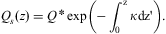 $${{Q}_s}\left( z \right)\: = \:Q\,^{\ast} \,\rm exp\left( {{\rm{ - }}\mathop{\int}\nolimits_{\!\!\!\!\!0}^z {\kappa dz{{\tf="TNR"\char"A9}}} } \right).\eqno\rm$$
Based on the measurement series at 60 cm depth, the magnitude of the attenuation coefficient was κ∼1 m-1. This corresponds to the transparency of surface ice and mixture of liquid water and slush. In the hard ice beneath the lake the attenuation is expected to be larger if there are sediments or gas bubbles, but smaller for clear ice.
Scales of supraglacial lakes based on physics
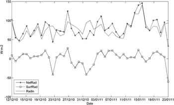
Simple physical principles can be employed to obtain the basic characteristics of supraglacial lakes. First, the lake growth and close-up seasons can be defined on the basis of the radiation balance by Q H > 0 and Q H < 0, respectively, where Q H is the surface radiation balance (Eq. (2)) plus the penetrating solar radiation, Q H = Q 0 + Q*. In the following discussion, the lake growth season and close-up season values are denoted below by the lower indexes + and −, respectively. Figure 8 shows the key radiation components for the evolution of the lake. The net radiation as well as the radiation penetrating into the lake (i.e. sunlight) varied within 50–150 W m-2, while the surface balance was between -50 and +20 W m-2. In 3–20 January the surface balance was slightly positive for a longer time, indicating the thinning of the surface ice layer.
Radiation balance from 12 December 2010–22 January 2011 in lake Suvivesi. NetRad = net radiation, SurfRad = surface radiation balance, and Radin = solar radiation penetrating into the lake body.

The total net radiation for lake growth is  $$--><$>{{\tilde{Q}}_{H + }}{{t}_ + }$$$, where the upper bar ∼ stands for averaging and t + is the length of the growth season. This corresponds to lake liquid water volume per unit area or the equivalent thickness of liquid water layer as:
 $$\tilde{H}\: = \:\frac{{{{{\tilde{Q}}}_{H + }}{{t}_ + }}}{{{{\rho }_w}L}},\eqno\rm$$
where ρw is water density and L is latent heat of freezing. Thus the lake depth is proportional to the mean solar radiation and the length of summer, with  $$--><$>{{\tilde{Q}}_{H + }}$$$ = 100 W m-2 and t + = 60 days,
 $$--><$>\tilde{H}\: = \:{\rm{1}}{\rm{.55}}\,{\rm{m}}$$$. Solar radiation is relatively high in the study region during summer since the sky is mostly clear. The energy needed to raise the temperature of ice from -15°C to 0°C is only 10% of the energy to melt the ice.
In the lake closure season (Q H < 0), the air temperature T a is below the freezing point, and then the ice growth is obtained from Zubov's law (Zubov Reference Zubov1945, see also Leppäranta Reference Leppäranta2009):
 $$h\: = \:\sqrt {aS\: + \:{{b}^2} } {\rm{ - }}b,\eqno\rm$$
where S is the sum of freezing-degree-days, and a ≈ 11 cm2 day-1 °C-1 and b ≈ 10 cm are the model parameters. In exact terms, a = 2k/(ρL), where k is thermal conductivity and ρ is ice density, and b = k/K a, where K a is ice-air heat exchange coefficient when taking the heat transfer as K a(T 0–T a). Thus a depends on the physical properties of ice and varies very little, while b is a more free parameter as it is connected to the heat transfer from ice surface to atmosphere. In snow-free conditions, as here, K a is roughly proportional to the mean wind speed, and when also  $$--><$>\sqrt {aS} \: \gg \:b$$$, the annual ice accumulation is not very sensitive to b:
 $$--><$>h\: \approx \:\sqrt {aS} {\rm{ - }}b$$$. With ten months close-up season and mean air temperature of -15°C (Kärkäs Reference Kärkäs2004), we have S = 4500 °C·day and thus h = 2.13 m. In addition, the lake also loses heat to the deeper ice sheet. Taking the temperature gradient as 1°C m-1 beneath the lake, the heat loss would be 2 W m-2. In ten months this corresponds to 18 cm ice growth. Ice thickness is approximately
 $$--><$>h\: \approx \:\sqrt {a\tilde{T}t} $$$, where
 $$--><$>\tilde{T}$$$ is mean air temperature (°C) and t is time, and hence (apart from thin ice cover in temperate climate zone) it is not very sensitive to temperature variations. In the present case, ±3°C overall change in the air temperature would change the ice thickness only ±20 cm. The exchange of heat with the underlying ice sheet is quite stable.
The summer and winter evolutions of the lake would change in a changing climate, toward a perennial lake or pure blue ice layer. Our scale analysis shows that in normal years the lake should freeze completely in winter. However, with an exceptionally warm summer and winter, a deep-water pocket could survive through the following winter season. The summer melt and winter ice growth become equal when:
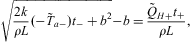 $$\sqrt {\frac{{2k}}{{\rho L}}({\rm{ - }}{{{\tilde{T}}}_{a{\rm{ - }}}}){{t}_{\rm{ - }}}\: + \:{{b}^2} } {\rm{ - }}b\: = \:\frac{{{{{\tilde{Q}}}_{H + }}{{t}_ + }}}{{\rho L}},\eqno\rm$$
where t− + t + = 1 year. With “>” or “ < ” inequality in Eq. (6), we have seasonal or perennial lakes, respectively. For no lake formation, the summer heat gain should be less than heat needed to raise the surface layer temperature to the melting point:  $$--><$>{{\tilde{Q}}_{H + }}{{t}_ + }\, \lt\,\:\rho c({\rm{ - }}{{\tilde{T}}_a}){{h}^\ast} $$$, where c is the specific heat of ice and h*∼1 m is a representative surface layer thickness of the ice sheet. The present climate is
 $$--><$>{{\tilde{T}}_{a{\rm{ - }}}}\:\sim \:{\rm{ - 15}}^{\circ}{\rm{C,}}\,{{t}_ + }\:\sim \:60\,{\rm{days,}}\,{{Q}_{H + }} \!\sim \!\:{\rm{100}} \, \:{\rm{W}}\, \:{{{\rm{m}}}^{{\rm{ - 2}}}} $$$, thus, the left side of Eq. (6) is 2.13 m and right side is 1.55 m. Increasing the winter temperature by 5°C would bring the left side to 1.72 m, increasing the summer length by 30 days would bring the left side to 2.01 m and the right side to 2.32 m, and increasing the summer heat balance by 50 W m-2 would also bring the right side to 2.32 m. Thus it is clear that how summer climate changes in future is critical to assessing whether these presently seasonal lakes can change to being perennial. Small increase in both summer length and summer heat balance would result in perennial lakes with positive feedback to further growth of the lakes.
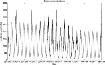
Next, consider the depth scale of the lake. The distribution of the solar energy with respect to depth depends on the transparency of the medium. The lake body has a good transparency. Figure 9 shows quantum scalar irradiance recorded with a spherical PAR sensor at a depth of 60 cm at ten minute intervals. These values can be converted to energy flux (in W m-2) by dividing by five (see Data collected section) and, assuming diffuse irradiance conditions, they need to be further divided by four to obtain the planar downwelling irradiance. The peak values in the first half of the record are about 2500 μmol m-2 s-1 and in the latter part 2000 μmol m-2 s-1. Daily averages were about 900–1200 μmol m-2 s-1. Using the albedometer measurements, the estimated attenuation coefficient is κ = 0.5–0.7 m-1.
Quantum scalar irradiance at a depth of 60 cm in lake Suvivesi in summer 2010–11. Date is given as day/month/year.

At depth z, the solar power absorption is Q* κexp(–κz), which suggests H = κ-1 as the natural depth scale. Furthermore, in time τ the porosity profile ν = ν(z) can be easily obtained if heat diffusion is ignored and a constant attenuation coefficient is assumed. Then, defining the lakewater body by ν(z) > ν0, the lake depth scale becomes:
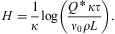 $$H\: = \:\frac{1}{\kappa }{\rm log}\left( {\frac{{Q^\,{^\ast}\,\kappa \tau }}{{{{\nu }_0}\rho L}}} \right).\eqno\rm$$
For κ∼0.6 m-1, Q*∼100 W m-2, τ∼60 days and ν0∼ $$\[--><$>\frac13<$><!--$$, we have H∼1.9 m. At ν > ν0, the strength of the ice becomes low and disappears, and the ice matrix changes into slush as observed. Thus the lake depth in the present study region scales as the inverse of the light attenuation coefficient.
The diffusive timescale across a distance  $$--><$> \rotate 16\ell $$$ is
 $$--><$>{{\tau }_{\! \rotate 16 \scale 50%\ell }\: {\rm{ = }}\:{{\rotate 16\ell }^{\rm{2}}} {\rm{(}}\rrho c{\rm{)/}}k$$$; it equals 38 days for
 $$--><$>\rotate 16\ell $$$ = 1.9 m. Consequently, solar radiation would alone open the lake to the depth of 1.9 m. The heat conduction law is written as:
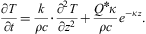 $$\frac{{\partial T}}{{\partial t}}\: = \:\frac{k}{{\rho c}} \cdot \frac{{{{\partial }^2} T}}{{\partial {{z}^2} }}\: + \:\frac{{{{Q}^{\rm{\ast}}} \kappa }}{{\rho c}}{{e}^{{\rm{ - }}\kappa z}}. \eqno\rm$$
In the lake growth problem we have ΔT∼10°C, depth scale of the thermally active layer is ∼10 m, and radiation scale is 100 W m-2. The thermally active layer is here understood as the layer where interannual variations in surface temperature are felt, having the thickness about 10 m (e.g. Paterson Reference Paterson1999). Thus the heat diffusion is ∼0.01°C day-1 while the radiational heating is ∼1.5°C day-1. Thus, solar radiation rapidly warms the lake with little diffusive loss and, once the melting begins, the heating rate Q* melts the ice by 2.8 cm day-1. Surface losses are small in summer compared to the heating of the lake body (see Fig. 8).
A steady state solution can be easily obtained for Eq. (8). Taking the boundary conditions as the surface temperature equal to T 0 and surface heat flux equal to Q 0, we have:
 $$T(z)\: = \:{{T}_0}{\rm{ - }}\frac{{{{Q}_0}\: + \:{{Q}^\ast} }}{k}z\: + \:\left( {{\rm{1 - }}{{{\rm{e}}}^{{\rm{ - }}\kappa z}} } \right)\frac{{{{Q}^\ast} }}{{\kappa k}}.\eqno\rm$$
The solution therefore consists of a linear contribution from surface heating and a modification by the depth-distributed solar heating. The scale of validity of this solution is up to the length of the steady state conditions. The longer the boundary conditions hold, the deeper the solution goes. For κ → ∞, sunlight is absorbed at the surface and its energy is added to the surface heating. For finite κ, there is a heating maximum beneath the surface when 0 < Q*+Q 0 < Q*, resulting in the lake body with a surface ice layer. The depth of the heated layer scales with κ-1. On 4 December 2010 (see above), when the lake was about to be born, there was a moist layer in 0.5–1 m depth at 0°C. The surface radiation balance was normally slightly positive but taking into account the latent heat loss it is clear that the surface heat balance was mostly negative and therefore the lake interior received the maximum heating during the summer.
Solar radiation is also the cause of the sub-structure in the lower lake layer and the slush pocket below the lake, because the light absorption coefficient is vertically not constant but varies primarily due to sediments in the ice. In a thin layer ΔH, the absorption of solar energy equals κΔHexp(–κz)Q*. The ratio of absorption in two consequent layers with absorption coefficients κ′ (lower) and κ (upper) is (κ′/κ)exp(–κΔH), which can be much greater than one, e.g. for κ′/κ = 2 and κΔH = 0.1, the ratio is 1.8. Thus the increased absorption of solar energy associated with sediment density offers a plausible explanation to the alternating deep slush and hard ice layers.
Conclusions
Supraglacial lakes in Dronning Maud Land, Antarctica have been examined using field observations from summers 2004–05 and 2010–11. Such lakes form in blue ice regions due to the melting caused by solar radiation penetrating into the surface layer of the ice sheet. Three lakes were mapped for their structure, and radiation budget measurements were made in one of them. All these lakes were located near a nunatak. Analytical modelling tools were employed to examine the scaling of the evolution, size and closing of supraglacial lakes. The following conclusions were drawn.
1) At the maximum development in January, the structures of the three supraglacial lakes were similar, showing two main layers, both ∼1 m thick. The upper layer had a thin (∼10 cm) surface ice layer on top of a thicker water body with some slush. The lower layer consisted of slush, soft ice and hard ice sub-layers, with a sediment-rich slush pocket at the bottom. Further below there was the hard ice sheet. Ice crystals in the lower layer and beneath the lake bottom were granular, with size 1–3 cm.
2) The supraglacial lakes started to form around 10–20 December and progressed in similar way in both years. The spatial structure showed that the lake formation starts from patches, which grow laterally and connect with each other to form the lakes.
3) The boundary zone of supraglacial lakes could be characterized as an ‘ice bog’ with soft and hard spots and ‘bogholes’. Sediments were found in bogholes and, due to their good light absorption properties, we assume that they act as the trigger for the formation of the bogholes. The formation of the bog structure is probably due to local variability in the heat budget as is also seen in the patchy structure of the melting process in ice-covered lakes in general.
4) The hydraulic conductivity in the bog and lake varied from 0.25 to 30 cm s-1. By a controlled experiment, the conductivity of closely packed slush mass was obtained as 6.3 cm s-1, which serves as a reference for assessing the integrity of the lake structure.
5) The lakewater was very clean. Electric conductivity was 1–10 μS cm-1 and pH ranged between 6 and 8. Sediment particles consisted of soil and gravel. The source of impurities was the neighbouring nunataks, from where they were transported by air. No systematic spatial variations were observed. Electric conductivity showed a decreasing trend during summer, and pH decreased in the first half of summer and increased in the second half.
6) Based on albedometer measurements and PAR sensor at a depth of 60 cm inside the lake body, the albedo of the lake ranged between 0.4–0.6 and the light attenuation coefficient was 0.5–0.7 m-1.
7) Analyses of the physics showed that the depth of supraglacial lakes scales with the light attenuation coefficient, and the volume of liquid water scales with the length of summer and solar heating. The formation of the lake body was possible because the timescale for diffusion of heat into the solid underlying ice sheet is too long to move the solar heat downward. In our study region, the liquid water layer thickness may reach 1.5 m, and winter freezing can, in theory, exceed 2 m depth. The lakes in the study region are, therefore, seasonal. To change into a perennial lake regime, the most sensitive factor is the integrated summer heating, which can be caused by increased heat flux and/or increased length of the summer season.
In a parallel study of the biology of lakes Suvivesi and Plogen, very low phytoplankton levels were observed in the summer 2010–11 (Keskitalo et al. unpublished data). Further work with the physics of these lakes will be directed to a detailed analysis of their heat budget based on observations and proceeding to a development of a mathematical model for their life history. Monitoring of lake Suvivesi summer structure, depth and size will continue. The main question is to further examine the spatial structure and its development. The results will serve as one excellent indicator of climate changes in the area. In particular, the lake formation tells much of the summertime radiation balance that is not very sensitive to air temperature.
Acknowledgements
We are grateful to the logistics team of the FINNARP 2004 expedition and to Anne Lehtinen for information on the conditions in summer 2003–04 in the study lakes. Mika Mäkelä is thanked for help in processing the ice samples. Funding was provided for our projects Seasonal snow in Antarctica II (2002–05) and Evolution of snow cover and dynamics of atmospheric deposits in the snow in the Antarctica (2009–12) by the Academy of Finland. The constructive comments of the reviewers are also gratefully acknowledged.