





1. Introduction
The stellarator is a device that confines plasma by generating a toroidal magnetic field, envisaged for the purpose of energy production by controlled fusion (Spitzer Reference Spitzer1958). The shaping of the magnetic field critically affects properties of the plasma, such as confinement time and pressure profiles.
We focus on quasi-poloidally symmetric magnetic fields with a negligible enclosed toroidal current. Such fields are a subset of quasisymmetric fields (Nührenberg & Zille Reference Nührenberg and Zille1988; Boozer Reference Boozer1995; Rodríguez et al. Reference Rodríguez, Helander and Bhattacharjee2020), which have a symmetry of the magnetic field strength such that the guiding-centre motion of the particles possesses a conserved canonical momentum, analogous to the axisymmetric, tokamak case. Quasisymmetry itself is a special case of omnigeneity, for which the bounce-averaged radial drift of the trapped particles vanishes (Hall & McNamara Reference Hall and McNamara1975). When omnigenous fields have poloidally closed contours of the magnetic field strength, they are called quasi-isodynamic (QI) (Gori, Lotz & Nührenberg Reference Gori, Lotz and Nührenberg1996). Quasi-poloidal (QP) symmetry is the particular case of quasisymmetry where the magnetic field strength is constant on poloidal loops, as opposed to toroidal (quasi-axisymmetry) or helical loops (quasi-helical symmetry). Quasi-poloidal symmetry is thus also a special case of QI symmetry.
Quasi-poloidal magnetic fields have advantages beyond those of other quasisymmetric and QI configurations. Given that the enclosed toroidal current of a QP flux surface vanishes, which is a good approximation for QP stellarators (QPS) due to vanishing bootstrap and Pfirsch–Schlüter currents, the field lines are geodesics of the surface. Consequently, the radial drift of guiding centres vanishes pointwise (Palumbo Reference Palumbo1968) – the ideal scenario for collisionless particle confinement. Hence, there is no radial neoclassical transport to first order in guiding-centre motion. For the same reasons, the bootstrap current vanishes (Landreman & Catto Reference Landreman and Catto2012). The Pfirsch–Schlüter current also vanishes (see, e.g. § 3.4), resulting in zero Shafranov (Reference Shafranov1963) shift and potentially higher beta limits. Reducing geodesic curvature has also been shown to improve electrostatic turbulence in QI stellarators (Roberg-Clark et al. Reference Roberg-Clark, Xanthopoulos, Plunk and Stroteich2026).
Furthermore, QP symmetry has the potential to reduce anomalous transport. Uniquely, there is a lower level of damping for poloidal flows (Shaing & Callen Reference Shaing and Callen1983). Thus, QP symmetry allows for shearing flows that can possibly suppress turbulence (Wobig Reference Wobig1999; Terry Reference Terry2000; Spong et al. Reference Spong, Hirshman, Lyon, Berry and Strickler2005; Alcuson et al. Reference Alcuson, Reynolds-Barredo, Bustos, Sanchez, Tribaldos, Xanthopoulos, Goerler and Newman2016), though this is yet to be verified. As a final advantage of QP symmetry, there is evidence that a second stability is possible in high-beta, compact, QP fields (Ware et al. Reference Ware, Westerly, Barcikowski, Berry, Fu, Hirshman, Lyon, Sanchez, Spong and Strickler2004), though this may not be a general feature of QP fields.
There has been recent success in optimising for QI fields with suitable properties for plasma confinement (Goodman et al. Reference Goodman, Camacho Mata, Henneberg, Jorge, Landreman, Plunk, Smith, Mackenbach, Beidler and Helander2023; Sánchez et al. Reference Sánchez, Velasco, Calvo and Mulas2023). Thus, stellarators with QI fields are now tenable candidates for fusion reactors (Hegna et al. Reference Hegna2025; Lion et al. Reference Lion2025). In designing a reactor, it is useful to understand the landscape of viable magnetic fields. Understanding QP fields further progresses this goal despite QP being a more restrictive assumption than QI.
Despite their attractive properties, QP magnetic fields are overlooked, often on the basis of two theoretical arguments. Firstly, there is a prevailing misconception (see, e.g. Garren & Boozer Reference Garren and Boozer1991) that if the radial drift vanishes pointwise, then the magnetic field strength must be constant on the flux surface, which is unreasonably constraining. This is not true however: QP flux surfaces with zero net toroidal current also have vanishing radial drift. As Palumbo (Reference Palumbo1968) first showed, given vanishing radial drift, the orthogonals to field lines must be symmetry directions of the field strength. If these orthogonals do not close on themselves, it does indeed follow that the field strength is a flux function. A QP surface circumvents this argument, since the orthogonals to the field lines do indeed close on themselves. Granted, the only explicitly known class of magnetic fields that has geodesic field lines is the Palumbo (Reference Palumbo1968) magnetic fields, which do have constant field strength on the flux surfaces and are the only axisymmetric fields with this property (Schief Reference Schief2003). Nonetheless, the lack (or impossibility) of exact analytical QP solutions does not preclude the attainment of very accurate, numerically generated QP magnetic fields.
Secondly, exact QP symmetry is impossible close to the magnetic axis. The proof of this is reproduced in Appendix A. However, this formal proof has limited relevance for practical stellarators. For low aspect ratio stellarators, the ‘near-axis’ region is generally much smaller than the volume enclosed by the last closed flux surface, though the region of validity of near axis can vary by configuration. For large aspect ratio stellarators, the level of QP breaking around the axis can be made asymptotically small. Nonetheless, the proof indicates that we cannot replicate the success of directly constructing approximate fields using a near-axis expansion, as is possible for QI symmetry and other forms of quasisymmetry (Landreman & Sengupta Reference Landreman and Sengupta2019; Plunk, Landreman & Helander Reference Plunk, Landreman and Helander2019; Camacho Mata, Plunk & Jorge Reference Camacho Mata, Plunk and Jorge2022; Jorge et al. Reference Jorge, Plunk, Drevlak, Landreman, Lobsien, Camacho Mata and Helander2022; Goodman et al. Reference Goodman, Camacho Mata, Henneberg, Jorge, Landreman, Plunk, Smith, Mackenbach, Beidler and Helander2023; Rodríguez et al. Reference Rodríguez, Sengupta and Bhattacharjee2023). In this work we provide an alternative analytical tool for constructing and understanding QP flux surfaces.
The principal result of this paper is a reduction of the problem of finding QP surfaces. Generally, to find a flux surface with desired properties, one has to solve a three-dimensional (3D) problem, as properties such as field strength and currents depend on field lines adjacent to the flux surface. In contrast, we show that one can solve a simpler two-dimensional (2D) problem in order to produce individual QP flux surfaces. This simpler problem is realised through the surface equations, presented in § 3.2. This framework achieves many of the simplifying features of a near-axis expansion. Firstly, it provides a reduced parametrisation of a QP surface, since only three 2D functions satisfying the surface equations need to be specified. These three functions are curvature, torsion and the ‘orthogonal distance’ between field lines. Furthermore, it represents a simplification of the equilibrium problem, since only three equations need to be solved. This streamlines the direct approach, where one instead needs to specify three 3D functions, e.g.
 $\boldsymbol{r}(l,\alpha ,\psi )$
for position vector
 $\boldsymbol{r}$
and coordinates
 $(l,\alpha ,\psi )$
, that solve an overdetermined set of equilibrium equations. In exchange for simplicity, this approach has limitations: it only guarantees a single QP surface and a surface found through this method need not enclose nested QP flux surfaces.
The outline of this paper is as follows. In § 2 we describe the magnetic field within a moving frame formalism. This is necessary for revealing the ensuing simplification. Readers primarily interested in results may skip the mathematical details of this section, but should note that much of the notation used in this paper is defined there. In § 3 we first define a local generalisation to QP surfaces, termed local QP (LQP) surfaces – the exact relationship to QP surfaces is discussed in § 3.1. In § 3.2 the main result is presented: a reduced, decoupled model for LQP surfaces, termed the surface equations. In § 3.3 we sketch how the surface equations can be used to formulate a simplified surface optimisation problem for finding QP surfaces, and in § 3.4 we discuss the physics of what makes QP flux surfaces susceptible to this simplification. In § 4 we note two canonical classes of solutions: generalised helicoids, with surfaces of revolution (magnetic mirrors) as a notable subtype, and Hasimoto surfaces, which are surfaces traced out by the self-induced motion of a vortex filament. In the case of toroidal Hasimoto surfaces, we develop a theory of the magnetic field strength (§ 4.1): we show that such surfaces in vacuum are flat mirrors (Velasco et al. Reference Velasco, Calvo, Sánchez and Parra2023) and derive governing equations for the field strength. In § 5 the surface equations are compared with numerical magnetic field configurations optimised for QP symmetry. We note that it is the surface equations that are directly checked, but not their application as a dimensional reduction. Local deviations from the surface equations correspond to where there is significant QP error (§ 5.3), anomalous parallel currents (§ 5.4) and deviations of field lines from geodesics (§ 5.5). Moreover, through the surface equations, we explain the prevalence of sharp cusps in these configurations (§ 5.3) and provide a possible explanation for high mirror ratios and narrow pinch points (§ 5.6) in certain types of optimised QPS.
Illustration of the Darboux frame on a flux surface (constant
 $\psi$
). Here
 $\boldsymbol{\hat {t}}$
is parallel to field lines (shown in dark blue) and lies in the tangent plane to the surface,
 $\boldsymbol{\hat {n}}$
is normal to the surface and
 $\boldsymbol{\hat {b}}=\boldsymbol{\hat {t}}\times \boldsymbol{\hat {n}}$
also lies in the tangent plane to the surface.

2. A moving frame representation of a magnetic field
In this section we consider a particular description of a solenoidal field
 $\boldsymbol{B}$
. We work in a field-line-following coordinate system
 $(l,\alpha ,\psi )$
, where
 \begin{align} \frac { \partial \boldsymbol{r}}{\partial l} &= \boldsymbol{\hat {t}}:=\frac {\boldsymbol{B}}{B} ,\\[-5pt]\nonumber \end{align}
 \begin{align} \boldsymbol{B}&=\boldsymbol{\nabla }\psi \times \boldsymbol{\nabla }\alpha , \end{align}
where we define the position vector
 $\boldsymbol{r}$
and the tangential unit vector
 $\boldsymbol{\hat {t}}$
. Such a field-line-following coordinate system always exists locally due to the Clebsch (Reference Clebsch1859) representation. In § 3 we adopt a specific choice of field-line-following coordinates when we consider LQP surfaces.
We expand vectors in the orthonormal frame
 $(\boldsymbol{\hat {t}},\boldsymbol{\hat {n}},\boldsymbol{\hat {b}})$
, where
 $\boldsymbol{\hat {n}}=\boldsymbol{\nabla }\psi / |\boldsymbol{\nabla }\psi |$
is the surface normal and the binormal is
 $\boldsymbol{\hat {b}} = \boldsymbol{\hat {t}} \times \boldsymbol{\hat {n}}$
. This is the Darboux frame (Darboux Reference Darboux2000) of the surfaces given by the level sets of
 $\psi$
, i.e. the flux surfaces, with the frame orientated along field lines. This is shown in figure 1. Though we use the usual nomenclature, such flux surfaces are considered only locally at this stage.
We expand the covariant basis vectors in this frame, i.e.
 \begin{align} \frac {\partial \boldsymbol{r}}{\partial \alpha } &= \eta \boldsymbol{\hat {t}} + \rho \boldsymbol{\hat {b}},\\[-6pt]\nonumber \end{align}
 \begin{align} \frac {\partial \boldsymbol{r}}{\partial \psi } &= \lambda \boldsymbol{\hat {t}} + \mu \boldsymbol{\hat {n}}+\nu \boldsymbol{\hat {b}} \end{align}
for some
 $\eta ,\rho ,\lambda ,\mu$
and
 $\nu$
. We have used the fact that
 $\partial _\alpha \boldsymbol{r}\boldsymbol{\cdot } \boldsymbol{\nabla }\psi =0$
. In terms of these variables,
 $B=1/\mu \rho$
and
 $\boldsymbol{\nabla }\psi = \boldsymbol{\hat {n}}/\mu$
.
The variables
 $\eta ,\rho ,\lambda ,\mu$
and
 $\nu$
are not independent of each other: they constitute the metric in this coordinate system, so they are constrained by the fact that 3D Euclidean space is flat. Namely, the Riemann curvature tensor, which is a function of the metric, should vanish. Calculating such flatness conditions directly is algebraically cumbersome. Instead, we use the method of moving frames (Darboux Reference Darboux2000; Cartan Reference Cartan2001). Although seemingly circuitous, this method naturally provides the requisite variables for understanding the geometry of the flux surface as a surface embedded in 3D Euclidean space. Moreover, this method is utilised in § 3 for revealing a simplification for QP surfaces. In Appendix B we show the equivalence between the constraints that are derived below and the Riemann flatness conditions.
The Darboux frame
 $(\boldsymbol{\hat {t}},\boldsymbol{\hat {n}},\boldsymbol{\hat {b}})$
is orthonormal, smoothly varying in space, and is a complete basis, so we can define
 $\boldsymbol{K}=(K_1,K_2,K_3), \, \boldsymbol{\chi }=(\chi _1,\chi _2,\chi _3)$
and
 $\boldsymbol{\sigma }=(\sigma _1,\sigma _2,\sigma _3)$
such that
 \begin{align} \frac {\partial }{\partial l}\begin{pmatrix} \boldsymbol{\hat {t}} \\[2pt] \boldsymbol{\hat {n}} \\[2pt] \boldsymbol{\hat {b}} \\[2pt] \end{pmatrix} & = \begin{pmatrix} 0 & \quad -K_3 & \quad K_2 \\[2pt] K_3 & \quad 0 & \quad -K_1 \\[2pt] -K_2 & \quad K_1 & \quad 0 \end{pmatrix} \begin{pmatrix} \boldsymbol{\hat {t}} \\[2pt] \boldsymbol{\hat {n}} \\[2pt] \boldsymbol{\hat {b}} \\[2pt] \end{pmatrix},\\[-10pt]\nonumber \end{align}
 \begin{align} \frac {\partial }{\partial \alpha }\begin{pmatrix} \boldsymbol{\hat {t}} \\[2pt] \boldsymbol{\hat {n}} \\[2pt] \boldsymbol{\hat {b}} \\[2pt] \end{pmatrix} & = \begin{pmatrix} 0 & \quad -\chi _3 & \quad \chi _2 \\[2pt] \chi _3 & \quad 0 & \quad -\chi _1 \\[2pt] -\chi _2 & \quad \chi _1 & \quad 0 \end{pmatrix} \begin{pmatrix} \boldsymbol{\hat {t}} \\[2pt] \boldsymbol{\hat {n}} \\[2pt] \boldsymbol{\hat {b}} \\ \end{pmatrix},\\[-10pt]\nonumber \end{align}
 \begin{align} \frac {\partial }{\partial \psi }\begin{pmatrix} \boldsymbol{\hat {t}} \\[2pt] \boldsymbol{\hat {n}} \\[2pt] \boldsymbol{\hat {b}} \\[2pt] \end{pmatrix} & = \begin{pmatrix} 0 & \quad -\sigma _3 & \quad \sigma _2 \\[2pt] \sigma _3 & \quad 0 & \quad -\sigma _1 \\[2pt] -\sigma _2 & \quad \sigma _1 & \quad 0 \end{pmatrix} \begin{pmatrix} \boldsymbol{\hat {t}} \\[2pt] \boldsymbol{\hat {n}} \\[2pt] \boldsymbol{\hat {b}} \\ \end{pmatrix}. \end{align}
These equations can be thought of as a generalisation of the Frenet–Serret formulas (Serret Reference Serret1851; Frenet Reference Frenet1852). Relative to the field lines on the flux surface,
 $-K_3$
is the normal curvature,
 $K_2$
is the geodesic curvature and
 $K_1$
is the geodesic torsion (Eisenhart Reference Eisenhart2013). The anti-symmetry of the matrices follows from the orthonormality of the frame.
Compatibility of these equations in flat space requires that the partial derivatives applied to the Darboux frame commute. For example,
 $\partial _l \partial _\alpha (\boldsymbol{\hat {t}},\boldsymbol{\hat {n}},\boldsymbol{\hat {b}}) = \partial _\alpha \partial _l (\boldsymbol{\hat {t}},\boldsymbol{\hat {n}},\boldsymbol{\hat {b}})$
. This leads to
 \begin{align} \boldsymbol{\chi }_l - \boldsymbol{K}_\alpha &= \boldsymbol{K} \times \boldsymbol{\chi },\\[-10pt]\nonumber \end{align}
 \begin{align} \boldsymbol{K}_\psi - \boldsymbol{\sigma }_l &= \boldsymbol{\sigma } \times \boldsymbol{K},\\[-10pt]\nonumber \end{align}
 \begin{align} \boldsymbol{\sigma }_\alpha - \boldsymbol{\chi }_\psi &= \boldsymbol{\chi } \times \boldsymbol{\sigma }, \end{align}
where the subscripts denote partial derivatives. This is consistent with intuition in flat space: vectors parallel transported in closed loops should return to the same vector, so partial derivatives applied to vectors should commute.
Furthermore,
 $\boldsymbol{r}_{l\alpha }=\boldsymbol{r}_{\alpha l}$
gives
 \begin{align} \eta _l &= K_2 \rho ,\\[-10pt]\nonumber \end{align}
 \begin{align} \chi _3 &= K_3 \eta - K_1 \rho ,\\[-10pt]\nonumber \end{align}
 \begin{align} \chi _2 &= K_2 \rho + \rho _l. \end{align}
Similarly,
 $\boldsymbol{r}_{l\psi }=\boldsymbol{r}_{\psi l}$
gives
 \begin{align} \lambda _l &= K_2 \nu - K_3 \mu ,\\[-10pt]\nonumber \end{align}
 \begin{align} \mu _l &= K_3 \lambda - K_1 \nu -\sigma _3,\\[-10pt]\nonumber \end{align}
 \begin{align} \nu _l &= K_1\mu - K_2 \lambda +\sigma _2. \end{align}
Finally,
 $\boldsymbol{r}_{\alpha \psi }=\boldsymbol{r}_{\psi \alpha }$
gives
 \begin{align} \eta _\psi - \lambda _\alpha &= \sigma _2 \rho + \chi _3 \mu - \chi _2 \nu ,\\[-10pt]\nonumber \end{align}
 \begin{align} \mu _\alpha &= \sigma _1 \rho - \sigma _3 \eta + \chi _3 \lambda - \chi _1 \nu ,\\[-10pt]\nonumber \end{align}
 \begin{align} \rho _\psi - \nu _\alpha &= \chi _2 \lambda - \chi _1 \mu -\sigma _2 \eta . \end{align}
Finding
 $\eta ,\rho ,\lambda ,\mu ,\nu ,\boldsymbol{K},\boldsymbol{\chi }$
and
 $\boldsymbol{\sigma }$
that satisfy (2.4)–(2.7) in some domain
 $\mathcal{D}_{(l,\alpha ,\psi )}$
is equivalent to specifying a solenoidal field
 $\boldsymbol{B}$
in the real-space domain
 $\mathcal{D}_{\boldsymbol{r}}$
that corresponds to integrating the covariant basis vectors ((2.1a
) and (2.2)) over
 $\mathcal{D}_{(l,\alpha ,\psi )}$
. In the subsequent sections, we consider further properties of the magnetic field in terms of these variables.
For future reference, we also write the current
 $\boldsymbol{J}= \boldsymbol{\nabla }\times \boldsymbol{B}$
as
 \begin{align} \boldsymbol{J} & = \frac {1}{\mu \rho } \bigg [ \left ( \left (\frac {1}{\mu \rho }\right )_\alpha -\left (\frac {\eta }{\mu \rho }\right )_l \right ) \frac {\partial \boldsymbol{r}}{\partial \psi } \nonumber\\[5pt]& \quad + \left ( \left (\frac {\eta }{\mu \rho }\right )_\psi -\left (\frac {\lambda }{\mu \rho }\right )_\alpha \right ) \frac {\partial \boldsymbol{r}}{\partial l} + \left ( \left (\frac {\lambda }{\mu \rho }\right )_l-\left (\frac {1}{\mu \rho }\right )_\psi \right ) \frac {\partial \boldsymbol{r}}{\partial \alpha } \bigg ], \end{align}
which can be derived using the expression for the curl in general coordinates (see, e.g. Chapter 5 in Imbert-Gerard, Paul & Wright Reference Imbert-Gerard, Paul and Wright2024).
3. A reduced model for LQP surfaces
We define a LQP surface as a flux surface where
-
(i) the field lines are geodesics,
-
(ii) the current normal to the surface is zero, and
-
(iii) the current parallel to the field lines is zero.
These properties depend only on the local (albeit 3D) details of the magnetic field, whereas QP is a global property of a toroidal magnetic field. Nonetheless, LQP surfaces are the appropriate local generalisation of QP surfaces: force-balanced QP magnetic fields with zero enclosed toroidal current have LQP flux surfaces, with the precise relationship discussed in § 3.1. We note that flux surfaces in magnetic mirror geometry can also be LQP surfaces.
Independently of the relationship with QP surfaces, LQP surfaces are worthy of consideration on physical grounds. The fact that the current normal to the surface vanishes is a trivial consequence of magnetohydrostatic (MHS) force balance,
 \begin{align} \boldsymbol{J}\times \boldsymbol{B}=\boldsymbol{\nabla }p(\psi ), \end{align}
where we assume a scalar pressure. If the field lines are geodesics of the flux surface, the radial drift in the guiding-centre approximation vanishes pointwise, resulting in no radial neoclassical transport and no bootstrap current to first order in guiding-centre motion. The Pfirsch–Schlüter current also vanishes for geodesic field lines, so the plasma does not generate its own parallel currents; hence, it is reasonable to further assume that the parallel current is zero. Indeed, this has its own merits: negligible parallel current improves MHD stability and is one of the intrinsic advantages of a stellarator over a tokamak (Helander et al. Reference Helander2012).
The main result of this section – and indeed of the paper – is introduced in § 3.2, where we present a surprisingly simple model for producing LQP surfaces. We also sketch how this model can be used to independently generate QP surfaces (§ 3.3) and discuss the physics that makes LQP surfaces amenable to such simplification (§ 3.4).
3.1. Relation to QP symmetry
We start by examining LQP surfaces. By definition, field lines are geodesics of the surface if the geodesic curvature
 $K_2$
vanishes. Physically, this is because the ‘acceleration’ term
 $\partial \boldsymbol{\hat {t}}/\partial l$
has no component in the tangent plane of the surface, spanned by
 $(\boldsymbol{\hat {t}},\boldsymbol{\hat {b}})$
, as can be seen from (2.3a
). By (2.5a
), this implies that
 $\eta _l=0$
, and we can therefore change coordinates from
 $(l,\alpha )$
to
 $(l',\alpha )$
by shifting the origin of the field lines,
 \begin{align} l' := l - \int ^\alpha \text{d}\alpha ' \, \eta (\alpha ',\psi ). \end{align}
It is noted that in a toroidal geometry, one has to exercise care in extending the
 $(l,\alpha )$
coordinates globally, but this transformation introduces no novel issues, since it is merely a statement of where we choose to define
 $l=0$
(Imbert-Gerard et al. Reference Imbert-Gerard, Paul and Wright2024). For instance, if
 $2\pi \psi$
is the enclosed toroidal flux then we can restrict
 $\alpha \in [0,2\pi )$
and pick the lower limit of the integral in (3.2) to be
 $0$
. Equation (3.2) then implies that
 $\eta '=0$
, where
 $\eta '$
is defined as in (2.2) but now with respect to
 $(l',\alpha ,\psi )$
coordinates. This choice of coordinates is a particular example of geodesic coordinates (see, e.g. Eisenhart Reference Eisenhart2013). The coordinates
 $l'$
and
 $\alpha$
are orthogonal on the surface, since
 $(\partial _\alpha \boldsymbol{r})_{l'} = \rho ' \boldsymbol{\hat {b}}$
is perpendicular to
 $(\partial _{l'}\boldsymbol{r})_\alpha = \boldsymbol{\hat {t}}$
. Henceforth, we work in such coordinates, so we drop the prime on
 $l',\eta '$
, etc. Thus, the geodesic condition on LQP surfaces simply becomes
 $\eta =0$
.
Additionally, by definition, the current normal to the LQP surfaces vanishes. Thus, by (2.8), we conclude that
 \begin{align} \left (\mu \rho \right )_\alpha = 0 \end{align}
or equivalently that
 $\partial B/\partial \alpha = 0$
. This symmetry of the field strength is simply quasisymmetry. Indeed, we define the quasisymmetry vector as the covariant basis vector
 $\boldsymbol{u}=\partial _\alpha \boldsymbol{r} = \rho \boldsymbol{\hat {b}}$
. Then, using the quasisymmetry definition of Rodríguez et al. (Reference Rodríguez, Helander and Bhattacharjee2020), it follows that locally
 \begin{align} \boldsymbol{u}\boldsymbol{\cdot } \boldsymbol{\nabla }B &= 0,\\[-6pt]\nonumber \end{align}
 \begin{align} \boldsymbol{u}\times \boldsymbol{B} &= \boldsymbol{\nabla }\psi ,\\[-6pt]\nonumber \end{align}
 \begin{align} \boldsymbol{\nabla }\boldsymbol{\cdot }\boldsymbol{u} &= 0. \end{align}
Equation (3.4a
) follows from
 $B=1/\mu \rho$
and (3.3). Equation (3.4b
) follows from
 $\boldsymbol{u}=\rho \boldsymbol{\hat {b}}$
,
 $\boldsymbol{B}=\boldsymbol{\hat {t}}/\mu \rho$
,
 $\boldsymbol{\hat {b}}\times \boldsymbol{\hat {t}}=\boldsymbol{\hat {n}}$
and
 $\boldsymbol{\nabla }\psi = \boldsymbol{\hat {n}}/\mu$
. Note that (3.4b
) usually has an additional minus sign, but we define
 $\boldsymbol{u}$
such that
 $\rho \gt 0$
and
 $(\boldsymbol{\hat {t}},\boldsymbol{\hat {n}},\boldsymbol{\hat {b}})$
forms a right-handed coordinate system. Equation (3.4c
) follows from
 $\boldsymbol{\nabla }\boldsymbol{\cdot }\boldsymbol{u} = \partial _\alpha (\mu \rho )/ \mu \rho =0$
. It is notable that we did not have to assume quasisymmetry; it emerged naturally from assuming geodesic field lines and zero current normal to the surfaces and revealed itself in geodesic coordinates.
We now demonstrate why QP surfaces are natural choices for LQP surfaces. We prove that, given a toroidal surface with zero enclosed toroidal current and pointwise zero normal current, the field lines are geodesics on that surface if and only if the magnetic field strength on the surface has QP symmetry.
Firstly, we prove the forward direction: geodesic field lines imply QP symmetry. We have already shown that LQP surfaces are quasisymmetric, so they possess a symmetry vector
 $\boldsymbol{u}$
and a corresponding symmetry coordinate
 $\alpha$
. On a toroidal surface where
 $B$
is not constant on a flux surface, the integral curves of
 $\boldsymbol{u}$
must close, according to (3.4a
). The integral of
 $\boldsymbol{B}$
around a closed
 $\boldsymbol{u}$
integral curve (denoted
 $\partial S$
) must vanish because
 $\boldsymbol{u}\boldsymbol{\cdot }\boldsymbol{B}=0$
by the choice of geodesic coordinates, so
 \begin{align} 0=\oint _{\partial \mathcal{S}} \text{d}\alpha \, \frac {\partial \boldsymbol{r}}{\partial \alpha }\boldsymbol{\cdot }\boldsymbol{B}= \iint _{\mathcal{S}} \text{d}\boldsymbol{S} \boldsymbol{\cdot }\boldsymbol{J}, \end{align}
where the second equality follows from Stokes’ theorem. If
 $\partial \mathcal{S}$
closed toroidally then
 $\iint _S \text{d}\boldsymbol{S}\boldsymbol{\cdot }\boldsymbol{J}$
is the external poloidal current, which does not vanish. If
 $\partial \mathcal{S}$
closed poloidally then
 $\iint _S \text{d}\boldsymbol{S}\boldsymbol{\cdot }\boldsymbol{J}$
is the enclosed toroidal current, which does vanish. So,
 $\partial S$
as a poloidal curve is a possible solution. As a final possibility, if
 $\partial \mathcal{S}$
closed helically then
 $\iint _S \text{d}\boldsymbol{S}\boldsymbol{\cdot }\boldsymbol{J}$
is a linear combination between external poloidal and enclosed toroidal currents, which also does not vanish. So,
 $\partial \mathcal{S}$
must close poloidally. This yields QP symmetry.
The poloidal current exterior to the flux surface does not vanish, whereas the toroidal current enclosed by the flux surface does vanish.
We now show the backward direction: QP symmetry implies geodesic field lines, given zero enclosed toroidal current and
 $\boldsymbol{J}\boldsymbol{\cdot }\boldsymbol{\hat {n}}=0$
. By quasisymmetry and the vanishing of the normal current, we have
 $(\eta /\mu \rho )_l=0$
. For an irrational surface, this means that
 $\eta /\mu \rho$
is constant on the surface, since field lines get arbitrarily close to every point on the surface. For rational surfaces, assuming that the rotational transform is not constant and we have QP in an infinitesimal volume around the surface, we also have the fact that
 $\eta /\mu \rho$
is constant by continuity. Then, we integrate the magnetic field along the poloidal symmetry curve
 $\partial \mathcal{S}$
. Using the fact that the enclosed toroidal current vanishes and Stokes’ theorem, this integral vanishes:
 \begin{align} 0=\oint _{\partial \mathcal{S}} \text{d}\alpha \, \frac {\partial \boldsymbol{r}}{\partial \alpha }\boldsymbol{\cdot }\boldsymbol{B}= \oint _{\partial \mathcal{S}} \text{d}\alpha \, \frac {\eta }{\mu \rho }. \end{align}
As
 $\eta /\mu \rho$
is constant, this implies that
 $\eta =0$
, and consequently, that we have geodesic field lines.
In Appendix C we make the connection with Boozer (Reference Boozer1981) coordinates, which can be defined since
 $\boldsymbol{J}\boldsymbol{\cdot }\boldsymbol{\hat {n}}=0$
(Rodríguez et al. Reference Rodríguez, Sengupta and Bhattacharjee2021). We also show that, under the further assumption of MHS force balance, the parallel current on a QP surface vanishes whenever the enclosed toroidal current vanishes. Thus, we conclude from this subsection that QP symmetry is the natural global analogue for LQP surfaces. However, LQP surfaces, defined locally, constitute a larger class of possible surfaces, toroidal or not (e.g. magnetic mirrors).
3.2. The surface equations
In this subsection we present a reduced, decoupled model for single LQP flux surfaces. We first discuss what it means to have defined a single LQP surface in the language of the moving frame.
A magnetic field is exactly described by
 $\eta ,\rho ,\lambda ,\mu ,\nu ,\boldsymbol{K},\boldsymbol{\chi }$
and
 $\boldsymbol{\sigma }$
as functions of
 $(l,\alpha ,\psi )$
, provided that the geometric constraints of § 2 are obeyed. In contrast, a single flux surface, taken as an embedded surface in real space, is precisely described by
 $\eta ,\rho ,\boldsymbol{K}$
and
 $\boldsymbol{\chi }$
as functions of
 $(l,\alpha )$
, provided that (2.4a
) and (2.5) are satisfied. This result of classical differential geometry is referred to as Bonnet’s theorem (see, e.g. § 3.6 in Struik Reference Struik1950). A magnetic field requires additional information because it is a 3D bundle of field lines, whereas a single flux surface is a 2D manifold.
Even if we consider only a single LQP flux surface, finding an LQP surface is in principle a 3D problem. This is because defining the field strength and current on a flux surface requires information about field lines away from that surface. For the field strength, given
 $B= 1/(\mu \rho ) = 1/(\boldsymbol{r}_l\boldsymbol{\cdot }\boldsymbol{r}_\alpha \times \boldsymbol{r}_\psi )$
, we need to know field lines in the infinitesimal neighbourhood of the surface, i.e. we need to know
 $\boldsymbol{r}(l,\alpha ,\psi _0+\delta \psi )$
to first order in
 $\delta \psi$
, where
 $\psi _0$
labels the relevant flux surface.
In general, describing currents on a flux surface requires information about field lines further from the surface, i.e.
 $\boldsymbol{r}(l,\alpha ,\psi _0+\delta \psi )$
to two orders in
 $\delta \psi$
. This is manifest in the expression (2.8) for the current as terms like
 $\mu _\psi$
depend on
 $\boldsymbol{r}_{\psi \psi }$
(see (2.2b
)). However, when the field lines are geodesics on the surface, one requires information only about field lines in the immediate infinitesimal neighbourhood, i.e. to first order in
 $\delta \psi$
, to define the currents normal to the surface and parallel to the field lines. This is because when
 $\eta =0$
on the flux surface, which is the geodesic condition in geodesic coordinates as described in § 3.1, there are no terms involving
 $\boldsymbol{r}_{\psi \psi }$
contributing to the normal and parallel current, as can be seen from (2.8).
Therefore, to define a single LQP surface, we need to define a particular
 $\boldsymbol{r}(l,\alpha ,\psi _0+\delta \psi )$
to first order in
 $\delta \psi$
. In other words, a single LQP surface is defined by field lines on and directly adjacent to that surface. Geometrically, defining such field lines is equivalent to providing
 $\lambda ,\mu ,\nu $
and
 $\boldsymbol{\sigma }$
on the surface as functions of
 $(l,\alpha )$
at fixed
 $\psi =\psi _0$
and
 $\boldsymbol{K},\boldsymbol{\chi },\rho $
and
 $\eta$
as functions of
 $(l,\alpha ,\psi )$
for
 $\psi$
in the immediate neighbourhood of
 $\psi _0$
, provided that (2.4), (2.6) and (2.7) hold at
 $\psi =\psi _0$
and (2.5) holds for
 $\psi =\psi _0+\delta \psi$
for infinitesimal, arbitrary
 $\delta \psi$
. Solving these equations for those variables merely provides the requisite structure; an LQP surface must also satisfy the physical constraints of having (i) geodesic field lines, (ii) zero normal current, and (iii) zero parallel current:
 \begin{align} \eta &= 0 \quad \text{for } \psi =\psi _0+\delta \psi ,\\[-10pt]\nonumber \end{align}
 \begin{align} (\mu \rho )_\alpha &= 0\quad \text{for } \psi =\psi _0,\\[-10pt]\nonumber \end{align}
 \begin{align} \lambda _\alpha &= 0 \quad \text{for } \psi =\psi _0. \end{align}
The first equation corresponds to having geodesic field lines and choosing
 $(l,\alpha )$
to be geodesic coordinates (as discussed in § 3.1). We do not just impose
 $\eta =0$
on the relevant flux surface, but also in the neighbourhood of the flux surface. This reflects the requirement that a finite volume of surfaces possess the physical benefits of geodesic field lines. The second equation corresponds to zero normal current and is equivalent to quasisymmetry (also discussed in § 3.1). Given the previous two equations, the third equation corresponds to zero parallel current on the relevant flux surface.
We note one crucial simplification arising from field lines being geodesics. By (2.5a
), we deduce that
 $K_2=0$
. Thus, the Darboux frame on the surface reduces to the Frenet–Serret frame for the field lines, since (2.3a
) becomes the Frenet–Serret formulae (Serret Reference Serret1851; Frenet Reference Frenet1852). To comply with the usual notation, we replace ‘
 $\boldsymbol{K}$
’ with the curvature
 $\kappa := -K_3$
(equal to the normal curvature) and torsion
 $\tau := -K_1$
. We note that the curvature defined in this way can be negative, precisely when the principal normal of the field lines is anti-aligned with the surface normal.
We have determined the relevant variables and equations for finding a single LQP surface using the moving frame formalism. In Appendix D we manipulate and reduce these equations to obtain the main result of this paper: the geometry of a single LQP flux surface is determined by the solution to the surface equations
 \begin{align} \kappa _\alpha &= -2\rho _l \tau - \rho \tau _l,\\[-10pt]\nonumber \end{align}
 \begin{align} \tau _\alpha &= \rho _l \kappa + \left ( \frac {\rho _{ll}-\rho \tau ^2}{\kappa } \right )_l,\\[-14pt]\nonumber \end{align}
 \begin{align} \left ( \frac {\kappa }{\rho }\right )_\alpha &= 0. \end{align}
For the reader who skipped to these equations, we reiterate that
 $\kappa$
is the signed curvature of the field lines,
 $\tau$
is the torsion of the field lines,
 $(l,\alpha )$
are a particular choice of field-line-following coordinates where
 $\partial _\alpha \boldsymbol{r}=\boldsymbol{u}$
is the quasisymmetry vector, and
 $\rho =|\boldsymbol{u}|$
is the ‘orthogonal distance’ between the field lines.
The surface equations have three remarkable properties. Firstly, the surface equations depend only on the geometry of the flux surface and the field lines on that flux surface (through the variables
 $(\rho ,\kappa ,\tau )$
); they do not depend on field lines away from the flux surface. How can this be if the field strength and currents on the flux surface depend on field lines away from the flux surface? This is because of a second remarkable property: given a solution to the surface equations (representative of an embedded surface foliated by field lines), there exist (at least locally) some neighbouring field lines that would confer upon the surface the relevant LQP properties of zero normal and parallel currents. We show this mathematically by providing a set of equations that (along with the surface equations) are equivalent to the original problem for finding an LQP surface, and then showing that these equations admit a solution. These equations are derived alongside the surface equations in Appendix D and are presented here:
 \begin{align} \eta &= 0,\\[-10pt]\nonumber \end{align}
 \begin{align} K_2 &=0,\\[-10pt]\nonumber \end{align}
 \begin{align} \chi _1 &= -\frac {\rho _{ll}-\rho \tau ^2 }{\kappa },\\[-10pt]\nonumber \end{align}
 \begin{align} \chi _2 &= \rho _l,\\[-10pt]\nonumber \end{align}
 \begin{align} \chi _3 &= \rho \tau ,\\[-10pt]\nonumber \end{align}
 \begin{align} \lambda _\alpha &= 0,\\[-10pt]\nonumber \end{align}
 \begin{align} \lambda _l &= \kappa \mu ,\\[-10pt]\nonumber \end{align}
 \begin{align} \nu _l &= \frac {\rho _l}{\rho }\nu - 2 \tau \mu ,\\[-10pt]\nonumber \end{align}
 \begin{align} \mu _\alpha &= - \frac {\rho _\alpha }{\rho }\mu ,\\[-10pt]\nonumber \end{align}
 \begin{align} \sigma _1 &= - \frac {\rho _\alpha }{\rho ^2} \mu - \tau \lambda - \frac {\nu }{\rho }\frac {\rho _{ll}-\rho \tau ^2}{\kappa },\\[-10pt]\nonumber \end{align}
 \begin{align} \sigma _2 &= \frac {\rho _l}{\rho }\nu -\tau \mu ,\\[-10pt]\nonumber \end{align}
 \begin{align} \sigma _3 &= -\mu _l -\kappa \lambda + \tau \nu ,\\[-10pt]\nonumber \end{align}
 \begin{align} \rho _\psi &= \nu _\alpha + \rho _{l} \lambda + \frac {\rho _{ll}-\rho \tau ^2}{\kappa } \mu ,\\[-10pt]\nonumber \end{align}
 \begin{align} \eta _\psi &= 0,\\[-10pt]\nonumber \end{align}
 \begin{align} \kappa _\psi &= \mu _{ll} + (\kappa ^2 + 3 \tau ^2)\mu + \kappa _l \lambda + \frac {\kappa _\alpha }{\rho }\nu ,\\[-10pt]\nonumber \end{align}
 \begin{align} \tau _\psi &= \frac {\tau _\alpha }{\rho }\nu + \tau _l \lambda + \frac {\rho _\alpha }{\rho ^2}\mu _l + \left ( \left ( \frac {\rho _\alpha }{\rho ^2}\right )_l - 2 \frac {\tau }{\rho } \frac {\rho _{ll}-\rho \tau ^2}{\kappa } \right )\mu ,\\[-10pt]\nonumber \end{align}
 \begin{align} K_{2\psi } &= 0,\\[-10pt]\nonumber \end{align}
 \begin{align} \chi _{1\psi } &= -\left (\frac {\rho _{ll}-\rho \tau ^2}{\kappa } \right )_\psi ,\\[-10pt]\nonumber \end{align}
 \begin{align} \chi _{2\psi } &= \rho _{l \psi },\\[-10pt]\nonumber \end{align}
 \begin{align} \chi _{3 \psi } &= (\rho \tau )_\psi . \end{align}
These equations apply at fixed
 $\psi =\psi _0$
. Taken together with the surface equations, they enforce the relevant physical and geometric conditions. We now justify why these equations are solvable, given a solution
 $(\rho ,\kappa ,\tau )$
to the surface equations. First, we consider the variables
 $(\lambda ,\mu ,\nu )$
. They are determined by the homogeneous, linear differential equations (3.9f
)–(3.9i
). By the Frobenius (Reference Frobenius1877) theorem, there exists a solution
 $(\lambda ,\mu ,\nu )$
to these differential equations. This is because equations (3.9f
) and (3.9g
) are compatible: both equations agree that
 $\lambda _{\alpha l}=0$
, since
 $(\kappa \mu )_\alpha =0$
by the surface equation (3.8c
) and the quasisymmetry condition, presented here as (3.9i
). To uniquely specify a solution to these equations, certain boundary conditions must be specified:
 $\mu$
as a function of
 $l$
at fixed
 $\alpha$
(which corresponds to choosing the field strength; see § 3.4),
 $\nu$
as a function of
 $\alpha$
at fixed
 $l$
and
 $\lambda$
at a particular point. There is less freedom to specify boundary conditions in
 $\lambda$
because it is controlled by two equations, (3.9f
) and (3.9g
). The remaining functions
 $(\eta ,K_2,\boldsymbol{\chi },\boldsymbol{\sigma },\rho _\psi ,\eta _\psi ,\tau _\psi ,\boldsymbol{K}_\psi ,\boldsymbol{\chi }_\psi )$
are algebraically and compatibly determined in terms of
 $\rho ,\kappa ,\tau ,\lambda ,\mu$
and
 $\nu$
by (3.9a
)–(3.9e
) and (3.9j
)–(3.9t
).
A solution to these equations, alongside a solution to the surface equations, represents a single LQP flux surface. This is because, as discussed, a single LQP surface is defined by field lines in an infinitesimal volume around that surface, or equivalently, by the functions
 $\lambda ,\mu ,\nu ,\sigma ,\boldsymbol{K}, \boldsymbol{\chi },\rho ,\eta ,\boldsymbol{K}_\psi , \boldsymbol{\chi }_\psi ,\rho _\psi $
and
 $\eta _\psi$
at fixed
 $\psi =\psi _0$
as functions of
 $(l,\alpha )$
. Thus, the problem of finding an LQP flux surface has been reduced to solving the surface equations, since the remaining part of the problem is solvable given a solution to the surface equations. It is surprising that we do not have an overdetermined system, despite the numerous equations involved. We discuss the physical reasons for this in § 3.4.
A third and final remarkable property of the reduction to the surface equations is that
 $(\rho ,\kappa ,\tau )$
completely determine the surface and the field lines on it. Intuitively, this is clear:
 $(\kappa ,\tau )$
determine the field lines individually and
 $\rho$
tells us the spacing between the field lines. Formally, we can recall Bonnet’s theorem (stated at the start of this subsection) and note that
 $\boldsymbol{\chi }$
is algebraically determined by
 $(\rho ,\kappa ,\tau )$
through (3.9c
)–(3.9e
). The relevant compatibility conditions (2.4a
) and (2.5) are satisfied identically when
 $\boldsymbol{\chi }$
is expressed in this way, with the exception of two components of (2.4a
), which are equivalent to the first two surface equations. Thus, the first two surface equations are purely geometric conditions, as viewed by geodesics. Curiously, the physics of vanishing normal and parallel current reduces to the simple equation (3.8c
).
To summarise this subsection, the problem of finding an LQP surface has been reduced from a 3D problem to a 2D problem, since we need only solve the surface equations for the geometry of an embedded surface. An LQP surface is defined by its properties of field strength and currents, which depend on field lines away from the surface. However, once we have a solution to the surface equations, we can locally guarantee that there exist neighbouring field lines that would give that surface the relevant properties of an LQP flux surface, viz. zero parallel and normal currents. We can make this guarantee because the variables that define the neighbouring field lines can be found by solving a well-posed set of equations. In this sense, the surface equations are decoupled and complete. Appendix E makes a connection with the language of classical differential geometry for the reader who is fluent in such a language.
Finally, we comment on MHS force balance (3.1), which depends on the current in the binormal direction (perpendicular to the field lines and tangential to the flux surface). This component of current has not yet been considered and need not vanish, unlike the parallel and normal components of current. By substituting the expression (2.8) for the current into MHS force balance (3.1), we find that
 \begin{align} \mu _\psi = -\frac {\rho _\psi }{\rho }\mu + p'(\psi ) \rho ^2 \mu ^3 - \rho \mu ^2 \left ( \frac {\lambda }{\mu \rho }\right )_l. \end{align}
Because we look for a solution on a single surface, (3.10) does not lead to overdetermination, since
 $\mu _\psi$
was unconstrained by the system of equations in (3.9). Physically, this is because the current in the binormal direction is affected by field lines even further from the surface. Formally, the presence of
 $\mu _\psi$
in the expression for this component of the current implies that one requires
 $\boldsymbol{r}(l,\alpha ,\psi _0+\delta \psi )$
to two orders in
 $\delta \psi$
to define
 $\boldsymbol{J}\boldsymbol{\cdot }\boldsymbol{\hat {b}}$
on the flux surface
 $\psi =\psi _0$
. For a single LQP flux surface, these ‘far away’ field lines do not affect the parallel or normal currents, so we can choose them to satisfy MHS force balance on the relevant surface: hence, there is no overdetermination by imposing force balance when considering a single LQP flux surface. This is a fortunate and unique scenario: typically in studies of MHS equilibria, imposing MHS force balance on a quasisymmetric equilibrium creates overdetermination (Garren & Boozer Reference Garren and Boozer1991; Sengupta et al. Reference Sengupta, Nikulsin, Buller, Madan, Paul, Nies, Kaptanoglu, Hudson and Bhattacharjee2024). Moreover, (3.10) implies that
 $(\mu \rho )_{\psi \alpha }=0$
, which is just a statement of quasisymmetry in the neighbourhood of the surface. Therefore, all considerations thus far, including the surface equations, are consistent with a finite-beta equilibrium. However, it must be cautioned that (3.10) does determine the allowable size of
 $\delta \psi$
for which the present description is accurate.
3.3. A sketch for solving the surface equations through optimisation
In this subsection we sketch how the surface equations could be solved as an optimisation problem for generating LQP flux surfaces. This could be used as part of a larger optimisation for generating a practical QPS field or for quickly and efficiently generating flux surfaces to study trends in QP equilibria. This approach would be intrinsically faster than usual MHD equilibrium solvers (e.g. VMEC, Hirshman & Whitson Reference Hirshman and Whitson1983 or DESC, Dudt & Kolemen Reference Dudt and Kolemen2020) because we do not need to directly solve for MHD equilibrium within a 3D volume. For concreteness, we take the example of a toroidal QP flux surface, but a similar process could be designed for the generation of asymmetric magnetic mirror flux surfaces with the desirable properties of an LQP surface.
Computationally, we work in the coordinate system
 $(\vartheta ,\varphi )$
, where
 $\varphi$
is some particular toroidal angle coordinate and
 $\vartheta$
is some particular poloidal angle coordinate. The flux surface is parameterised by the single-valued functions
 $R(\vartheta ,\varphi )$
and
 $Z(\vartheta ,\varphi )$
, where
 $R$
and
 $Z$
correspond to the usual cylindrical coordinates with respect to an axis passing through the centre of the torus. In practice, one could work in discrete Fourier modes of
 $(\vartheta ,\varphi )$
, e.g.
 $R_{mn}$
, up to some chosen level of precision.
On the toroidal surface, we also parameterise a foliation of closed poloidal loops. In an exact QP solution, these would correspond to lines of constant
 $l$
(in the geodesic coordinates used throughout this paper). Equivalently, in an exact QP solution, they are the field lines for the field
 $\boldsymbol{u}=\partial _\alpha \boldsymbol{r}$
or the loops along which the magnetic field strength would be constant (though we do not solve for the magnetic field strength in this 2D problem). We take the poloidal loops to be level sets of some function
 $\varLambda (\vartheta ,\varphi )$
, which is necessarily periodic in
 $\vartheta$
. The field lines are taken as perpendicular to these poloidal loops. For specificity, we could take
 $\varLambda$
to be the distance along a chosen field line from some reference poloidal loop. In the solved problem where the field lines are geodesics, this
 $\varLambda$
becomes independent of the chosen field line and is equivalent to our choice of arc length coordinate
 $l$
.
We generate LQP flux surfaces by solving the surface equations as an optimisation problem. The free parameters are the surface, through
 $R(\vartheta ,\varphi )$
and
 $Z(\vartheta ,\varphi )$
, and the poloidal loops, through the function
 $\varLambda (\vartheta ,\varphi )$
. The function
 $\varLambda (\vartheta ,\varphi )$
is constrained to have level sets that close poloidally. The cost function,
 $f[\varLambda ,R,Z]$
, has two parts,
 $f_1[\varLambda ,R,Z]$
and
 $f_2[\varLambda ,R,Z]$
, where
 $f_1[\varLambda ,R,Z]=0$
ensures that the field lines are geodesics and if
 $f_2[\varLambda ,R,Z]=0$
also, the third surface, (3.8c
), is solved. We now consider these two parts in more detail.
Firstly, we enforce that the field lines are geodesics. The tangent vector to the field lines
 $\boldsymbol{\hat {t}}$
is obtained by calculating the orthogonal to the poloidally closed level sets of
 $\varLambda$
, a calculation that depends on
 $R$
and
 $Z$
. Then, using the tangent vector field
 $\boldsymbol{\hat {t}}$
, the geodesic curvature can be calculated, in a way that likewise depends on
 $R$
and
 $Z$
and is also calculable via well-established methods. The field lines are geodesics if and only if the geodesic curvature is zero everywhere, so we take this part of the cost function to be
 \begin{align} f_1[\varLambda ,R,Z] = \int _0^{2 \pi } \text{d}\vartheta \int _0^{2 \pi } \text{d}\varphi \,\sqrt {g}_{\text{surf}} \, |\kappa _g|, \end{align}
where
 $\kappa _g \equiv K_2$
is the geodesic curvature and the surface Jacobian
 $\sqrt {g}_{\text{surf}}$
ensures the integral is a surface average.
The second part of the cost function is connected with the third surface equation (3.8c
) and is somewhat more subtle. We define the field line label
 $\tilde {\alpha }$
to be constant along the magnetic field lines and go from
 $0$
to
 $2 \pi$
(for specificity) along the closed poloidal loops. We then take
 $s$
to be the arc length along the closed poloidal loop and define
 $\tilde {\rho } := \partial s/\partial \tilde {\alpha }$
. For the third surface equation, we must also calculate the normal curvature
 $\kappa _n \equiv -K_3$
from
 $\boldsymbol{\hat {t}}$
. When the geodesic curvature is zero, the normal curvature is the same as the curvature
 $\kappa$
.
We take the second part of the cost function to be
 \begin{align} f_2[\varLambda ,R,Z] = \int _0^{2 \pi } \text{d}\vartheta \int _0^{2 \pi } \text{d}\varphi \,\sqrt {g}_{\text{surf}}\, \left |\left ( \ln \frac {\kappa _n}{\tilde {\rho }}\right )_{l \tilde {\alpha }}\right |. \end{align}
To justify this expression, we show that precisely when
 \begin{align} \left ( \ln \frac {\kappa }{\tilde {\rho }}\right )_{l \tilde {\alpha }}=0, \end{align}
there exists a transformation
 $\alpha =f(\tilde {\alpha })$
such that the third surface equation (3.8c
) is satisfied. To show this, we suppose that (3.13) is true. Then,
 \begin{align} \left ( \ln \frac {\kappa }{\tilde {\rho }}\right )_{ \tilde {\alpha }}=g(\tilde {\alpha }) \end{align}
for some particular
 $g$
. We define
 $\alpha = f(\tilde {\alpha })$
. It follows that
 $\rho = \tilde {\rho } ({\text{d}f}/{\text{d} \tilde {\alpha }})$
. We choose
 $f$
to be
 \begin{align} f(\tilde {\alpha })= \int _0^{\tilde {\alpha }} \text{d}a \, \exp \left ( \int _0^a \text{d}b \, g(b)\right )\!, \end{align}
where
 $f$
has all the necessary features of a transform between periodic coordinates. First, it is monotonic; second, for
 $\tilde {\alpha }$
increasing by a period, which is
 $2\pi$
here for specificity,
 $f$
increases by a fixed amount. This relies on
 $\int _0^{2\pi } \text{d} \tilde {\alpha } \; g(\tilde {\alpha })=0$
, which follows from (3.14) and the fact that
 $\kappa$
and
 $\tilde {\rho }$
are single valued. Since
 $f$
solves the differential equation
 \begin{align} \frac {\text{d}^2 f}{\text{d} \tilde {\alpha }^2} = \frac {\text{d}f}{\text{d} \tilde {\alpha }} g(\tilde {\alpha }), \end{align}
the third surface equation (3.8c
) is satisfied. In the 2D picture, there is a ‘gauge’ freedom
 $\alpha \rightarrow f(\alpha )$
(corresponding to
 $\rho \rightarrow \rho /f'(\alpha )$
) in the orthogonal coordinate
 $\alpha$
, but the third surface equation (3.8c
) still imposes a non-trivial constraint, through (3.13).
We do not need to verify the first two surface equations, (3.8a
) and (3.8b
). These are identically satisfied when the field lines are geodesics, with
 $\kappa =\kappa _n$
and
 $\rho \rightarrow \tilde {\rho }$
. Indeed, these two surface equations are purely geometric constraints and are satisfied by any geodesic foliation of an embedded surface. In this set-up, the geometry is encoded through
 $R(\vartheta ,\varphi )$
and
 $Z(\vartheta ,\varphi )$
.
We also note that in practice, solving for
 $f_2[\varLambda ,R,Z]=0$
makes sense only if the field lines are sufficiently close to geodesics (i.e.
 $\kappa _n \gg \kappa _g$
). In a computational optimisation problem, this could be achieved by including the
 $f_2$
part only when
 $f_1$
is sufficiently small. Moreover, there could be numerical issues with the logarithm in (3.12). If geodesic curvature is close to zero everywhere (i.e.
 $f_1$
is sufficiently small), then normal curvature is likely to only be zero on isolated points or curves, lest the surface have flat regions. In any case, the integrand can be transformed to regularise these possible issues, e.g. by using
 $|( \tanh (\ln ( {\kappa _n}/{\tilde {\rho }})))_{l \tilde {\alpha }}|$
instead.
In practice, once a toroidal surface has been selected by this method, it can be used as the boundary for a complete equilibrium solver. In vacuum, the boundary shape completely determines the magnetic field inside the boundary. However, because of the locality of the assumptions behind LQP surfaces, there is no guarantee that there are nested QP flux surfaces within the boundary of a surface selected by this method. In this case, a second optimisation, using the equilibrium solver, could be used to fine tune the boundary surface to give the desired global properties. This approach has reasons to be better than existing methods for selecting initial conditions for QP symmetry. For instance, a heuristic, near-axis construction (such as that devised by Goodman et al. Reference Goodman, Camacho Mata, Henneberg, Jorge, Landreman, Plunk, Smith, Mackenbach, Beidler and Helander2023 and applied to QP surfaces in Haque et al. Reference Haque, Paul, Giuliani, Campagna, Madan and Sengupta2026) necessarily contains deviations from exact QP symmetry, since QP symmetry is not possible through the near-axis expansion. The current framework is not limited to the near axis. Nonetheless, it remains as future work to verify whether this approach can indeed lead to improved QP quality.
3.4. What is so special about LQP surfaces?
There are two unique features of LQP surfaces that lead to the drastic simplification of the surface equations. Indeed, such a reduction cannot be found generally. If we were to impose only quasisymmetry as a physical constraint (i.e. only (3.7b )), the moving frame formalism would lead to equations that are highly coupled and overdetermined. In such cases, describing the magnetic field through a moving frame is not particularly useful.
The first special feature is that, for LQP surfaces, the surface geometry is decoupled from the magnetic field strength. In the case of general quasisymmetry with zero normal current,
 $\boldsymbol{u}\boldsymbol{\cdot }\boldsymbol{B}=\eta /\mu \rho$
is constant on a flux surface (Rodríguez et al. Reference Rodríguez, Helander and Bhattacharjee2020). This couples a quantity that influences the geometry of the flux surface,
 $\eta$
, with a quantity that is determined by field lines in the neighbourhood of the surface, namely the field strength
 $1/\mu \rho$
. Local QP surfaces avoid this coupling by having geodesic field lines, which implies that
 $\eta =0$
everywhere. Notably, given a single LQP surface, it is always possible to construct another LQP surface with the same flux surface shape but a different magnetic field strength profile (so long as
 $\partial B/\partial \alpha =0)$
. This is because we can take a complete solution to the LQP equations (3.8) and (3.9), and construct another solution through
 $\mu \rightarrow g(l) \mu$
for arbitrary function
 $g$
.
There is a second way in which LQP surfaces are special. Without assuming geodesic field lines, the general expression for the parallel current in the moving frame representation is
 \begin{align} J_\parallel = \frac {1}{\mu \rho } \left ( \left ( \frac {\eta }{\mu \rho } \right )_\psi -\left ( \frac {\lambda }{\mu \rho } \right )_\alpha \right ) + \frac {\eta }{\mu \rho } \left ( \left ( \frac {\lambda }{\mu \rho } \right )_l -\left ( \frac {1}{\mu \rho } \right )_\psi \right ), \end{align}
where we have continued to assume that the normal current vanishes. As an aside, the second set of terms is the Pfirsch–Schlüter current, which vanishes for geodesic field lines (
 $\eta =0$
). For
 $\eta =0$
, the expression for the parallel current ceases to depend on
 $\mu _\psi$
. This means that, for the particular case of geodesic field lines, the parallel current is determined only by field lines in the immediate neighbourhood of the surface, not by field lines at second order from the surface. Despite being more restrictive – there are fewer field lines that can contribute to having zero parallel current – this fact leads to mathematical simplification, since the equations are decoupled from field lines that are not in the immediate neighbourhood of the surface. In other words, in the general non-geodesic case, we have to consider a ‘thicker’ volume around the surface in order to evaluate the parallel current, which means there are more variables coupled into the equations (though optimistically, this also represents increased freedom). It is also this fact that means our single LQP surface can always be force balanced without additional overdetermination, since the binormal current
 $\boldsymbol{J}\boldsymbol{\cdot }\boldsymbol{\hat {b}}$
can be manipulated without affecting the parallel current, by altering field lines further from the surface through
 $\mu _\psi$
, in accordance with (3.10).
4. Two fundamental classes of solutions to the surface equations
We have thus far considered only local details of the magnetic field, except in § 3.3, where we used the surface equations to define a reduced optimisation problem for finding toroidal QP flux surfaces. Here, we analytically apply global considerations to the surface equations. In this section we identify two natural classes of solutions to the surface equations: the first contains ‘magnetic mirrors’ as a solution, and the second has attractive and analytically tractable field strength properties.
We consider searching for toroidal, QP solutions. A toroidal QP surface is foliated by closed poloidal loops. Along these loops, the magnetic field strength is constant, the covariant basis vector
 $\partial _\alpha \boldsymbol{r}$
(also the quasisymmetry vector) is tangent, and the field lines are orthogonal. In the
 $(l,\alpha )$
coordinate system, these loops are given by
 $l=\text{const}$
. (In § 3.3, these poloidal loops were part of the free parameters for the optimisation problem.) We take
 $L$
to be the distance along a field line until it returns to the same poloidal loop, this value being independent of the chosen field line. Equivalently,
 $L$
is the distance along a field line between
 $\phi =0$
and
 $\phi =2 \pi$
for Boozer angle
 $\phi$
, as defined in Appendix C.
Thus, for a toroidal QP surface,
 $\rho$
,
 $\kappa$
and
 $\tau$
are periodic in
 $\alpha$
, but are generally aperiodic in
 $l$
, given a field line that does not close on itself. These functions are single valued in real space, so they are also constrained by the fact that
 $(l+L,\alpha )$
and
 $(l,\alpha + 2\pi \iota )$
are the same point on the surface, where we define the rotational transform
 $\iota$
. Unfortunately, beyond these necessary features, there are no a priori constraints on
 $\rho$
,
 $\kappa$
and
 $\tau$
that would ensure a toroidal surface. Thus, one either has to impose a numerical optimisation scheme that enforces toroidicity, such as that described in § 3.3, or check post facto whether a solution to the surface equations is a toroidal surface.
We now proceed in attempting to find analytic, toroidal QP solutions. From the first and third surface equations (3.8a ) and (3.8c ), we have the ‘conservation law’
 \begin{align} \frac {\partial }{\partial \alpha } \left ( \frac {\rho \kappa }{2}\right ) +\frac {\partial }{\partial l} ( \rho ^2 \tau )=0. \end{align}
We integrate this equation around one of the closed poloidal loops, which gives
 \begin{align} \oint \text{d}\alpha \, \rho ^2 \tau = C, \end{align}
where
 $C$
is some constant, and we have used the fact that
 $(\rho ,\kappa ,\tau )$
are single valued. We define
 $\gamma := \kappa /\rho$
, which is independent of
 $\alpha$
by the third surface equation (3.8c
). Then,
 \begin{align} \oint \text{d}\alpha \, \kappa ^2 \tau = C\gamma ^2. \end{align}
The left-hand side of this equation is invariant under
 $l \rightarrow l+L$
, since
 $\kappa$
and
 $\tau$
are single valued, so
 $\gamma (l)$
is periodic with period
 $L$
. This is evidently true for an irrational surface, which is where
 $\iota$
is an irrational number. This is because
 $(l+L,\alpha )$
and
 $(l,\alpha + 2\pi \iota )$
are the same point on the surface,
 $\gamma$
is smooth and independent of
 $\alpha$
, and positive integer multiples of an irrational, taken modulo
 $2\pi$
, are dense in
 $[0,2\pi ]$
.
The fact that
 $\gamma$
is periodic and
 $(\rho ,\kappa ,\tau )$
are generally aperiodic in
 $l$
couples periodic and aperiodic terms in the first two surface equations (3.8a
) and (3.8b
). This complicates the route to a global, toroidal solution, but a separation of variables can be achieved by substituting
 $\kappa = \rho \gamma$
. Then, we have
 \begin{align} \gamma &= -\frac {2\rho _l \tau + \rho \tau _l}{\rho _\alpha },\\[-10pt]\nonumber \end{align}
 \begin{align} \gamma _l &= \frac {K+\tau ^2}{\gamma \rho _l \rho -\tau _\alpha -({ K + \tau ^2})/{\gamma }}, \end{align}
where
 $K := -\rho _{ll}/\rho$
is the Gaussian curvature. Solving these two equations analytically in complete generality is not feasible, so we consider some natural classes of solutions. Given that
 $\gamma$
is periodic in
 $l$
, two natural classes emerge: (a)
 $(\rho ,\kappa ,\tau )$
are independent of
 $\alpha$
, and (b)
 $\gamma$
is constant.
An example of a generalised helicoid, with
 $\boldsymbol{r}= (-0.6 u^2 \cos b,-0.6 u^2 \sin b, u+ b )$
for
 $u \in [-2,2]$
and
 $b \in [0,2\pi ]$
. The magnetic field lines (shown in dark blue) are geodesics orthogonal to the helices given by
 $u=\text{const}$
. It should be cautioned that this surface is not poloidally closed, so it is not a fruitful solution for investigating QP surfaces.

Case (a) corresponds to generalised helicoids, as proved in Appendix F. An example is illustrated in figure 2. In the further special case where
 $\tau =0$
, we either have surfaces of revolution with the meridians as field lines (magnetic mirrors), as illustrated in figure 3, or the surface traced out by a planar curve translated in the direction of the curve’s binormal (i.e. surfaces of the form
 $z=f(x)$
with field lines given by
 $y=\text{const.}$
). These two cases are the only LQP surfaces where the torsion of the field lines is zero, even if we were to allow for
 $\alpha$
dependence. Notably, all LQP surfaces where
 $\boldsymbol{u}$
can be extended to a Killing vector of 3D Euclidean space reduce to case (a). This is also shown in Appendix F.
Thus, case (a) does not include any toroidal solutions. Nonetheless, in § 5 we see that numerically generated QP equilibria have sections that resemble magnetic mirrors, and in Appendix I we perturb around surfaces of revolution to qualitatively explain some properties of the toroidal equilibria.
An example of a surface of revolution, with
 $\boldsymbol{r}= ((1+ 0.9 \sin u) \cos b,(1+ 0.9 \sin u) \sin b, u )$
for
 $u \in [-2 \pi ,2 \pi ]$
and
 $b \in [0,2\pi ]$
. The field lines are the meridians, highlighted in dark blue.

We now consider case (b). In this case,
 $\rho \propto \kappa$
. We have the same physical situation under the simultaneous rescaling
 $\alpha \rightarrow C \alpha$
and
 $\psi \rightarrow \psi /C$
for arbitrary constant
 $C$
, so we can set
 $\gamma =1$
and
 $\rho =\kappa$
. With
 $\rho =\kappa$
, the first two surface equations (3.8a
) and (3.8b
) reduce to the Da Rios–Betchov equations (Da Rios Reference Da Rios1906; Betchov Reference Betchov1965), whilst the third equation (3.8c
) becomes trivial. Equivalently, using the definition of
 $\rho$
, we can model the field lines as obeying the vortex filament equation (also known as the localised induction approximation),
 \begin{align} \frac {\partial \boldsymbol{r}}{\partial \alpha } &= \kappa \boldsymbol{\hat {b}} \nonumber \\ &= \frac {\partial \boldsymbol{r}}{\partial l} \times \frac {\partial ^2 \boldsymbol{r}}{\partial l^2}, \end{align}
where the second line assumes that the principal normal and surface normal are in the same direction. If they are opposed, we still have the same physical equation, but under a ‘time reversal’
 $\alpha \rightarrow - \alpha$
. Surfaces traced out by a vortex filament are known as Hasimoto surfaces, and we appropriately adopt this term for describing LQP surfaces where
 $\rho \propto \kappa$
. Under the Hasimoto (Reference Hasimoto1972) map, the Da Rios–Betchov equations are equivalent to the nonlinear Schrödinger equation.
The authors are aware of one known class of irrational, toroidal, Hasimoto surfaces. This solution already has prominence in an analytic MHS equilibrium, viz. the Palumbo (Reference Palumbo1968) configuration. The Palumbo configuration (or class of configurations) is an axisymmetric torus, made up of nested toroidal Hasimoto flux surfaces, with constant field strength on each surface. Remarkably, the Palumbo configuration is exact for an entire volume (not just a surface) and obeys the MHS force balance throughout for an arbitrary pressure profile
 $p(\psi )$
. This series of toroidal Hasimoto surfaces is given by the periodic travelling wave solutions to the Da Rios–Betchov equations,
 $\kappa =\kappa (l+c\alpha )$
and
 $\tau = \tau (l+c\alpha )$
, as identified by Kida (Reference Kida1981). The equation for such surfaces is given in an MHS context by equation (5.26) in Schief (Reference Schief2003) and the surfaces are plotted in figure 1 therein. Unfortunately for our purposes, such surfaces, even when taken individually, cannot be QP, since the orthogonals to the geodesics wind helically and generally do not close. However, there may exist other toroidal Hasimoto surfaces that are consistent with QP surfaces, at least to an acceptable level of accuracy. In such a case, the magnetic field strength presents desirable features, as we show in the next subsection.
4.1. The magnetic field strength on toroidal Hasimoto surfaces
We have thus far ignored the magnetic field strength profile. This was because, as discussed in § 3.4, the question of field strength decouples from the question of surface geometry. However, with some additional weak assumptions, we can make further statements about the magnetic field strength on Hasimoto surfaces. We first establish a connection between Hasimoto surfaces and an attractive property for practical stellarators, termed the flat mirror property. We then derive an exact governing differential equation that determines the magnetic field strength profile in terms of the surface geometry quantities,
 $(\rho ,\kappa ,\tau )$
.
First, we show that a Hasimoto surface in vacuum is a flat mirror, as defined and studied in Velasco et al. (Reference Velasco, Calvo, Sánchez and Parra2023). Velasco et al. show that such magnetic fields exhibit small radial transport of energy and good confinement of bulk and fast ions. A flat mirror is defined as a QI magnetic field satisfying
 \begin{align} \partial _\psi \left ( B_{\text{max}} -B_{00}\right )=0 , \end{align}
where
 $B_{00}=\iint \text{d}\theta \text{d}\phi \, B/4\pi ^2$
, with
 $(\theta , \phi$
) as Boozer angles, defined in Appendix C, and
 $B_{\text{max}}$
is the maximum of the magnetic field strength on the surface.
In vacuum, we have
 $(\lambda /\mu \rho )_l = (1/\mu \rho )_\psi$
, as can be seen from the expression for the current (2.8) or equivalently by setting
 $p'(\psi )=0$
in the expression for MHS force balance (3.10). Using the fact that
 $B=1/\mu \rho$
is independent of
 $\alpha$
, we integrate this to find that
 \begin{align} \lambda = \frac {1}{B(l,\psi )} \int ^l \text{d}l' \partial _\psi B(l',\psi ) + \frac {f(\psi )}{B(l,\psi )}, \end{align}
where
 $f$
is the integration constant and is independent of
 $\alpha$
because we have
 $\lambda _\alpha = 0$
, as in (3.9f
). We now consider the transformation from
 $(l,\alpha ,\psi )$
coordinates to
 $(\phi ,\alpha ,\psi )$
, where
 $\phi$
is the toroidal Boozer angle. We thus have
 \begin{align} \left ( \frac {\partial }{\partial \psi }\right )_l &= \left ( \frac {\partial }{\partial \psi }\right )_\phi + \left (\frac {\partial \phi }{\partial \psi }\right )_l \left ( \frac {\partial }{\partial \phi }\right )_\psi\\[-10pt]\nonumber \end{align}
 \begin{align} &= \left ( \frac {\partial }{\partial \psi }\right )_\phi + \left ( \frac {1}{G} \int \text{d}l' \partial _\psi B(l',\psi ) \right ) \left ( \frac {\partial }{\partial \phi }\right )_\psi . \end{align}
The second equality follows from noting that in vacuum, the magnetic field can be written as
 $\boldsymbol{B}=G\boldsymbol{\nabla }\phi$
, where
 $G$
is constant. In other words,
 $G\phi$
is the magnetic potential for a vacuum magnetic field. Rearranging this expression and using
 $\partial _\phi = (G/B) \partial _l$
gives
 \begin{align} \left ( \frac {\partial }{\partial \psi }\right )_\phi = \left ( \frac {\partial }{\partial \psi }\right )_l - \lambda \left ( \frac {\partial }{\partial l}\right )_\psi , \end{align}
where we have absorbed the constant
 $f(\psi )$
into the choice of origin between
 $l$
and
 $\phi$
.
Now, we return to the fact that the current in the
 $\partial _\alpha \boldsymbol{r}$
direction vanishes:
 $(\lambda /\mu \rho )_l = (1/\mu \rho )_\psi$
. We combine this with (3.9g
) to find that
 \begin{align} \frac {\kappa }{\rho } &= (\partial _\psi - \lambda \partial _l ) B\\[-10pt]\nonumber \end{align}
 \begin{align} &= \left ( \frac {\partial B}{\partial \psi }\right )_\phi , \end{align}
where we have used (4.10) in the second equality. For a foliation of Hasimoto surfaces,
 $\kappa /\rho =\gamma (\psi )$
, so we find that
 \begin{align} B(\phi ,\psi ) = B_0(\psi ) + B_1(\phi ), \end{align}
where we use the fact that
 $B$
depends on only
 $\phi$
and
 $\psi$
. This arises from (3.7b
) and is equivalent to QP symmetry in the vacuum case considered here. We find that the magnetic field strength is separable into a radially varying part
 $B_0(\psi )$
and a surface-varying part
 $B_1(\phi )$
, which is constant across flux surfaces. As an even stronger constraint on the field strength, this satisfies the flat mirror condition (4.6). Technically, for the benefits of a flat mirror to be gained, it is required that
 $\partial _\psi B_{00}\gt 0$
(Velasco et al. Reference Velasco, Calvo, Sánchez and Parra2023). However, this can often be achieved by adding a finite plasma pressure, due to the plasma behaving diamagnetically. We have indeed concluded that vacuum foliations of Hasimoto surfaces, which are a subset of QP magnetic fields, are flat mirrors. It is important to note that this property does not follow from QP fields generally, but just this particular class of QP solutions. The optimisation problem sketched in § 3.3 can be easily modified to look for Hasimoto surfaces, which then provides a 2D method for investigating flat mirror QP configurations.
In addition to the flat mirror result, we now derive a differential equation for the magnetic field strength in terms of the surface geometry quantities. In principle, this allows us to express quantities of practical interest, such as the mirror ratio, in terms of the surface geometry. We assume that we have a toroidal Hasimoto surface and that
 $(\rho /\kappa )_{l \psi }=0$
, which is consistent with assuming that
 $\rho \propto \kappa$
in the neighbourhood of the Hasimoto surface. We do not assume here that we have vacuum. We first note that (3.9h
) can be written as
 \begin{align} \left (\frac {\nu }{\rho }\right )_l = -2 \frac {\mu \tau }{\rho }. \end{align}
Also, from (3.8c ), (3.9m ), (3.9o ), we have
 \begin{align} \left ( \frac {\nu }{\rho }\right )_\alpha = ( \partial _\psi - \lambda \partial _l) \ln \frac {\rho }{\kappa } + \left ( \frac {4 \tau ^2}{\kappa } + \kappa - \frac {\rho _{ll}}{\rho \kappa }\right ) \frac {1}{\rho B} + \frac {1}{\kappa } \left ( \frac {1}{\rho B}\right )_{ll}, \end{align}
where we have used
 $B=1/\mu \rho$
, which follows from the definition of the field-line-following coordinate system described in § 2. We now equate the
 $\alpha$
derivative of (4.14) with the
 $l$
derivative of (4.15) – another compatibility condition. This gives
 \begin{align} - \left ( \frac {2 \tau }{B \rho ^2}\right )_\alpha = \left [\left ( \frac {4 \tau ^2}{\kappa } + \kappa - \frac {\rho _{ll}}{\rho \kappa }\right ) \frac {1}{\rho B} + \frac {1}{\kappa } \left ( \frac {1}{\rho B}\right )_{ll} \right ]_l, \end{align}
where we have used the fact that
 $(\rho /\kappa )_l=0$
and
 $(\rho /\kappa )_{l \psi }=0$
, consistent with field lines obeying the vortex filament equation on the surface and in the neighbourhood of the surface. We now integrate this equation around an integral curve of
 $\boldsymbol{u}=\partial _\alpha \boldsymbol{r}$
, which is closed in toroidal geometry. Thus, as
 $2 \tau /B\rho ^2$
is single valued, the left-hand side vanishes and we have
 \begin{align} \left (\frac {1}{B}\right )_{ll}\oint \text{d}\alpha \frac {1}{\rho \kappa } -2 \left (\frac {1}{B}\right )_l \oint \text{d}\alpha \frac {\rho _l}{\kappa \rho ^2} + \frac {1}{B} \oint \text{d}\alpha \frac {1}{\rho \kappa }\left ( 4\tau ^2 + \kappa ^2 - \frac {2\rho _{ll}}{\rho } + \frac {2 \rho _l^2}{\rho ^2} \right ) = C, \end{align}
where
 $C$
is some constant and we have used
 $\partial _\alpha B = 0$
. The notable feature of this equation is that it establishes a direct relationship between the magnitude of the magnetic field and the geometry of the field lines, even though the exact nature of this relationship is obscure.
In this subsection we have used
 $\kappa /\rho = \gamma (\psi )$
not only on the surface but also in its neighbourhood. In doing so, extra consistency conditions arise by combining equations (3.9m
) and (3.9o
). We have not considered the consequences of enforcing this consistency.
5. Comparison with optimised numerical QP magnetic fields
In this section we present numerically generated vacuum QP magnetic fields, with the primary purpose of corroborating the surface equations. We caution the reader that we do not implement the proposed optimisation scheme of § 3.3, but optimise 3D fields for QP configurations, from which we compute the surface quantities. We present two sets of toroidal magnetic field configurations, with specifications detailed in table 1. These configurations were chosen because they are sufficiently varied to show the surface equations in different contexts, they exhibit sufficiently accurate QP fields to show regions where the surface equations are true, and they also fairly show where breakdowns can, and often do, occur.
We present specifications of the five numerical, QP equilibria, including the aspect ratio AR, the rotational transform
 $\iota$
on the boundary, the mirror ratio
 $R=(\text{max}(B)-\text{min}(B))/(\text{max}(B)+\text{min}(B))$
on the boundary and the number of field periods, NFP.

Table 1. Long description
Table listing 5 configurations and parameters: MHS solver, AR, iota, R, and NFP. Configurations 1–3 use DESC solver with AR between 11.36 and 14.12, and NFP of 2. Configurations 4–5 use SPEC solver with AR around 6.00 and NFP of 5.
The first three magnetic field configurations were produced and optimised for using the DESC code (Dudt & Kolemen Reference Dudt and Kolemen2020). Their boundary surfaces are displayed in figure 4. By the nature of the method for calculating the equilibrium field, this equilibrium necessarily has nested flux surfaces. Each configuration was produced by optimising for QP fields on the boundary (not throughout the whole volume), alongside an aspect ratio and rotational transform target on the boundary, and a vacuum target throughout the volume. The configurations were optimised via the proximal least-squares method. Furthermore, all configurations are converged, satisfying functional tolerance and gradient tolerance criteria. The weights in the objective function were chosen as the best performing from a set of five randomly generated sets. The initial condition for the optimisation came from the same class as that in § 3 of Goodman et al. (Reference Goodman, Camacho Mata, Henneberg, Jorge, Landreman, Plunk, Smith, Mackenbach, Beidler and Helander2023).
We also present two magnetic field configurations that were solved for by the SPEC code (Hudson et al. Reference Hudson, Dewar, Dennis, Hole, McGann, von Nessi and Lazerson2012). They were optimised for using the adjoint methods developed in Nies et al. (Reference Nies, Paul, Hudson and Bhattacharjee2022). These configurations are exactly vacuum throughout the whole volume, which comes at the cost of not necessarily having nested flux surfaces. As with the other set, these configurations were generated by optimising for QP fields on the boundary, alongside an aspect ratio and rotational transform target. The initial condition for the optimisation was a rotating ellipse with the desired aspect ratio and rotational transform, as predicted by Mercier (Reference Mercier1964). In both sets of configurations, the optimisation took place in steps, with successive increases to the number of boundary modes (Landreman & Paul Reference Landreman and Paul2022).
In the following subsections we comment on the quality of QP symmetry (§ 5.1), we detail how the surface equations are tested (§ 5.2) and then we explain deviations from the surface equations through the appearance of cusps (§ 5.3), non-zero parallel currents (§ 5.4) and loss of geodesicity (§ 5.5). Finally, we note the preference for high mirror ratios, double wells and narrow pinch points in § 5.6.
The boundary surface of the three configurations produced via DESC.

5.1. Quality of QP symmetry
We define the QP error on a surface of a configuration as
 \begin{align} \text{QP error}=\frac {\int _0^{2 \pi } \text{d}\vartheta \int _0^{2 \pi } \text{d}\varphi \sqrt {g}_{\text{surf}} ({1}/{B^3}) \left | \boldsymbol{B}\times \boldsymbol{\nabla }B \boldsymbol{\cdot } \boldsymbol{\nabla }\psi \right |}{\int _0^{2 \pi } \text{d}\vartheta \int _0^{2 \pi } \text{d}\varphi \sqrt {g}_{\text{surf}}}, \end{align}
where
 $2\pi \psi$
is the toroidal magnetic flux and
 $\int _0^{2 \pi } \text{d}\vartheta \int _0^{2 \pi } \text{d}\varphi \sqrt {g}_{\text{surf}} (\ldots )$
is an integral over the surface, given that
 $(\vartheta ,\varphi )$
are the computational poloidal and toroidal angle coordinates (not necessarily straight field-line coordinates) and
 $\sqrt {g}_{\text{surf}} = | \partial \boldsymbol{r}/\partial \vartheta \times \partial \boldsymbol{r}/\partial \varphi |$
is the surface Jacobian. This QP error is based on the commonly used ‘two-term’ formulation of quasisymmetry (see, e.g. Rodríguez et al. Reference Rodríguez, Paul and Bhattacharjee2022), but there is only one term because we aim for QP configurations that have zero enclosed toroidal current. The QP objective function used during the optimisations was slightly different to this QP error definition and is spelled out in Appendix G.
For the five configurations, we present the quality of QP symmetry as a function of the surface in figure 5. We also make the comparison with the magnetic field design for the proposed QPS experiment (Nelson et al. Reference Nelson2003; Spong et al. Reference Spong, Hirshman, Lyon, Berry and Strickler2005) and the vacuum, precise QA configuration of Landreman & Paul (Reference Landreman and Paul2022). For the latter, the error is appropriately adjusted to be
 \begin{align} \text{QA error}=\frac {\int _0^{2 \pi } \text{d}\vartheta \int _0^{2 \pi } \text{d}\varphi \sqrt {g}_{\text{surf}} ({1}/{B^3}) \left | \boldsymbol{B}\times \boldsymbol{\nabla }B \boldsymbol{\cdot }\boldsymbol{\nabla }\psi + ({G}/{\iota })\boldsymbol{B}\boldsymbol{\cdot }\boldsymbol{\nabla }B\right |}{\int _0^{2 \pi } \text{d}\vartheta \int _0^{2 \pi } \text{d}\varphi \sqrt {g}_{\text{surf}}}, \end{align}
where
 $2 \pi G$
is the external poloidal current.
In figure 5 we see that the level of QP error is significantly higher than that of the precise QA configuration, despite the DESCconfigurations representing an improvement over QPS. We do not intend for this work to represent the forefront of possible QP solutions (see Haque et al. (Reference Haque, Paul, Giuliani, Campagna, Madan and Sengupta2026) instead), as these solutions were generated for the purpose of corroborating the surface equations. Nonetheless, it seems that optimising for a QP configuration using standard methods is more difficult than for a QA or quasi-helical configuration. For solutions outside the region of validity of the near axis, this difficulty has not been explained. It might be due to a limitation of current optimisation methods, in which case the scheme of § 3.3 could lead to improved QP solutions. It may also be due to fundamental difficulties with QP configurations. Indeed, as we detail in § 5.3, there is a fundamental tension between the third surface equation and toroidicity that can lead to cusps in the surface.
The QP error (defined in (5.1)) for six different magnetic field configurations as a function of the flux surface and the QA error (defined in (5.2)) for one additional configuration. Configurations 1–3 were produced using DESC and configurations 4 and 5 were produced using SPEC (QP error plotted only on the boundary where a flux surface necessarily exists). Here `QPS’ corresponds to the magnetic field design for the QPS (Nelson et al. Reference Nelson2003; Spong et al. Reference Spong, Hirshman, Lyon, Berry and Strickler2005) and ‘precise QA’ corresponds to the configuration found in Landreman & Paul (Reference Landreman and Paul2022). Configurations 1–3 show an improvement over QPS. Despite QP error being only targeted on the boundary, there is a lower level of QP error towards the axis.

5.2. How the surface equations are tested
The first two surface equations, (3.8a ) and (3.8b ), are purely geometric and are satisfied by any embedded surface foliated by geodesic field lines. Thus, to verify the first two surface equations, it suffices to ensure that the geodesic curvature is negligible on the boundary surface. As it turns out, this is a direct target for the optimiser as the geodesic curvature is proportional to the LQP error on a surface:
 \begin{align} \frac {1}{B^3} \boldsymbol{B}\times \boldsymbol{\nabla }B \boldsymbol{\cdot }\boldsymbol{\nabla }\psi = \rho \kappa _g \end{align}
(cf. (5.1) and the optimiser objective functions presented in Appendix G). The fact that
 $\kappa _g \rightarrow 0$
leads to QP was explained in § 3.1: a surface with geodesic field lines, zero net enclosed toroidal current and zero normal current is necessarily QP symmetric. Despite being a direct target of the optimiser, deviations from zero geodesic curvature do exist and are significant, as demonstrated in § 5.3.
The third surface equation, (3.8c
), is assessed directly. For this, we need to interpret
 $\kappa$
,
 $\rho$
and
 $\partial _\alpha$
for our numerical equilibria. We take
 $\kappa$
to be the normal curvature,
 $\kappa _n$
. For calculating
 $\rho$
, we use the transformation to Boozer coordinates
 \begin{align} \theta &= \vartheta + \tilde {\lambda } + \iota \omega ,\\[-6pt]\nonumber \end{align}
 \begin{align} \phi &= \varphi + \omega , \end{align}
where
 $\tilde {\lambda }(\vartheta ,\varphi )$
gives the transformation to straight field-line coordinates and
 $\omega (\vartheta ,\varphi )$
gives the transformation from those coordinates to Boozer coordinates. Calculating
 $\tilde {\lambda }$
and
 $\omega$
from numerical equilibria is standard practice when provided with flux surfaces (since
 ${\boldsymbol{\nabla }}\psi$
can be straightforwardly defined). For the SPEC equilibria, there is no obvious globally defined
 $ \boldsymbol{\nabla }\psi$
since there are no nested flux surfaces; see Nies et al. (Reference Nies, Paul, Hudson and Bhattacharjee2022) for how
 $\tilde {\lambda }$
and
 $\omega$
are calculated in this case. In vacuum, the magnetic field can be written as
 $\boldsymbol{B}=G\boldsymbol{\nabla }(\omega + \varphi )$
, where
 $G$
is constant. Given the surface Jacobian
 $\sqrt {g}_{\text{surf}} = | \partial \boldsymbol{r}/\partial \vartheta \times \partial \boldsymbol{r}/\partial \varphi |$
, we then take
 $\rho$
to be
 \begin{align} \rho = \frac {\sqrt {g}_{\text{surf}} B}{G | (1+\omega _\varphi ) (1+ \tilde {\lambda }_\vartheta ) - \omega _\vartheta (\tilde {\lambda }_\varphi - \iota ) |}, \end{align}
where
 $\iota$
is the rotational transform. This agrees with the theoretical definition of
 $\rho$
when
 $\kappa _g=0$
, as shown in Appendix H.
Finally, for exact QP configurations, we have
 \begin{align} \left ( \frac {\partial }{\partial \theta } \right )_\phi = 0 \quad \iff \quad \left (\frac {\partial }{\partial \alpha }\right )_l=0, \end{align}
so the third surface equation is verified if and only if
 $\kappa /\rho$
depends only on
 $\phi$
. In figure 6 we illustrate what the plots of
 $\kappa _g$
and
 $\kappa /\rho$
on the boundary should look like for the surface equations to be verified.
A schematic example of what it looks like for the surface equations to be verified or falsified on a flux surface. For
 $\phi \lt \pi /2$
, there is agreement with the surface equations, since the geodesic curvature is zero and
 $\kappa /\rho$
only depends on
 $\phi$
. For
 $\phi \gt \pi /2$
, there is disagreement as the geodesic curvature is non-zero and
 $\kappa /\rho$
does not have vertical contours.

5.3. The appearance of cusps
We plot quantities for the first DESC configuration: (a)
 $\kappa /\rho$
and (b) the geodesic curvature
 $\kappa _g$
, both on the boundary surface as a function of Boozer angles, and (c) toroidal cross-sections of the boundary flux surface. Lengths are measured with respect to the average major radius. The black line in (a) and (b) is a field line. We see agreement with the third surface equation, except the regions with large geodesic curvature (i.e. where QP breaking is significant).

Figure 7. Long description
Panel A: A contour plot shows the geodesic curvature on the boundary surface as a function of Boozer angles. The x-axis represents the Boozer angle phi, and the y-axis represents the Boozer angle theta. The color scale on the right indicates the geodesic curvature values, ranging from -24 to 30. A black line represents a field line. Panel B: A heatmap displays the geodesic curvature on the boundary surface as a function of Boozer angles. The x-axis represents the Boozer angle phi, and the y-axis represents the Boozer angle theta. The color scale on the right indicates the geodesic curvature values, ranging from -2.16 to 2.16. A black line represents a field line. Panel C: A line plot shows toroidal cross-sections of the boundary flux surface. The x-axis represents the major radius R, and the y-axis represents the minor radius z. Different colors represent different values of the Boozer angle phi, as indicated by the legend on the right.
In this subsection we consider the first DESC magnetic field configuration. For this configuration, the vacuum target was essentially achieved. In figure 7(a) we see that
 $\kappa /\rho$
varies primarily horizontally in agreement with the third surface equation, except for regions of sharp vertical change around
 $\theta \approx 1$
and
 $\theta \approx 4.5$
for
 $\phi \in (0.75,2.5)$
. This does not falsify the third surface equation because these are precisely the regions where the geodesic curvature deviates significantly from zero, as can be seen from figure 7(b). After all, zero geodesic curvature was an assumption behind the derivation of the surface equations.
In fact, we can understand these deviations from the surface equations through the surface equations themselves. The curvature
 $\kappa$
is negative whenever the field line principal normal is opposed to the surface normal. Based on intuition from tokamaks, the inboard and outboard sides of the torus typically have opposite signs of
 $\kappa$
. However, the third surface equation tells us that
 $\kappa /\rho$
should be constant on poloidal loops, so
 $\kappa$
should not be able to change sign, since
 $\rho \gt 0$
. The optimiser rectifies this difficulty by isolating the regions where
 $\kappa$
changes sign to thin cusps, with
 $\kappa /\rho$
independent of
 $\theta$
only away from these cusps. The cusps are visible in figure 7(c) at
 $\phi \approx 0.5 \pi$
as the tips on the top and bottom of the cross-section. These cusps are also visible in figure 4 where the surface ‘curves around’.
We note that the cusps also appear to follow the field lines. This can be understood through MHS force balance. As the field is vacuum, it is necessarily force free, so the tension force from the field lines can only be balanced by magnetic pressure. The magnetic pressure can only grow so large given the limited field strength variation, so the magnetic tension force has to be minimised by not having field lines go across the cusp.
5.4. The effect of parallel current
We now consider the second DESC magnetic field configuration. In figure 8(a) we observe noticeable departure from the third surface equation, since the contours are largely not close to vertical. There are two related reasons for this.
For the second DESC configuration: (a)
 $\kappa /\rho$
, (b) the geodesic curvature
 $\kappa _g$
, and (c) the parallel current
 $J_\parallel$
. All quantities are plotted on the boundary surface as a function of Boozer angles. Lengths are measured with respect to the average major radius and the current is normalised by the mean magnetic field on the boundary. There are two related reasons for deviations from the third surface equation: areas of high geodesic curvature and large parallel current.

Firstly, consider the region
 $\phi \in (0.4,0.8)$
. This region of the surface is similar to the configuration considered in the last subsection: there are approximately straight contours separated by ‘cusps’, which is where the geodesic curvature is largest (see figure 8
b). The geodesic curvature deviates somewhat from zero even away from these cusps, which explains why the vertical contours are slightly curved and angled. As in the last subsection, we can explain the cusps by the fact that
 $\kappa$
typically has to change sign from the inboard to the outboard side, in contradiction with the third surface equation.
Now, consider the remaining portion of the surface:
 $\phi \in (0,0.4)$
and
 $\phi \in (0.8,2\pi /5)$
. The contours are not vertical here at all, despite the geodesic curvature being small. Here, it is another assumption of the surface equations that breaks down: the parallel current is non-zero. Zero current density was a target for the optimiser but was not sufficiently attained everywhere in this configuration.
Even without considering the vacuum target, having non-zero parallel current is somewhat unexpected. This is because of the theoretical result presented at the end of Appendix C: assuming QP symmetry, force-balance and zero net toroidal current, the parallel current should vanish pointwise. The magnetic field configuration presented in figure 8 does indeed have zero net toroidal current and is force balanced (as current perpendicular to the field lines is indeed negligible). Thus, it is deviations from the QP configuration (i.e. deviations from zero geodesic curvature) the leads to non-zero parallel currents. Curiously, the region where geodesic curvature is significant (
 $\phi \in (0.4,0.8)$
) is different to the region where parallel currents are significant: hence, this is a non-local effect.
5.5. When are field lines sufficiently geodesic?
In this subsection we use the third DESC magnetic field configuration to point out that the third surface equation is satisfied (locally) only if the field lines are sufficiently geodesic, in the sense that the geodesic curvature should be much smaller than the normal curvature.
For the boundary surface of the third DESC configuration: (a)
 $\kappa /\rho$
, (b) the geodesic curvature
 $\kappa _g$
, and (c) the logarithm of the geodesic curvature divided by normal curvature
 $\kappa _n$
. For the third surface equation to be true, the geodesic curvature should be small compared with the normal curvature, which is not the case within the overlaid black/white rectangles.

Figure 9. Long description
Panel A: A contour plot displays the ratio of geodesic curvature to normal curvature. The x-axis represents the variable phi ranging from 0 to 3.5, and the y-axis represents the variable theta ranging from 0 to 6. The color scale on the right indicates values from -28.8 to 36.0. Several black rectangles are overlaid on the plot, highlighting specific regions. Panel B: A heatmap shows the geodesic curvature. The x-axis represents the variable phi ranging from 0 to 3.5, and the y-axis represents the variable theta ranging from 0 to 6. The color scale on the right indicates values from -2.0 to 2.0. Several black rectangles are overlaid on the heatmap, highlighting specific regions. Panel C: A contour plot displays the logarithm of the geodesic curvature divided by normal curvature. The x-axis represents the variable phi ranging from 0 to 3.5, and the y-axis represents the variable theta ranging from 0 to 6. The color scale on the right indicates values from -7.2 to 9.0. Several black rectangles are overlaid on the plot, highlighting specific regions.
We consider two different parts of the boundary surface of this configuration. The region
 $\phi \in (1.3,\pi )$
is similar to the central region of the first configuration considered in § 5.3: the third surface equation is violated on field-line-following cusps (see figure 9
a), which is where the geodesic curvature (and thus QP error) is large, as per figure 9(b). Away from these cusps, the contours of
 $\kappa /\rho$
are nearly vertical.
We now consider the region
 $\phi \in (0,1.3)$
, where the magnetic field strength is largest. Apart from distinct blobs at
 $(\phi ,\theta )\approx (0.7,3)$
and at
 $(\phi ,\theta )\approx (0.7,5.5)$
, the geodesic curvature is relatively small in an absolute sense, as per figure 9(b). These blobs can also be thought of as cusps, and also represent areas where the third surface equation does not hold (contours of
 $\kappa /\rho$
are not vertical). However, even away from these blobs, the contours are not close to vertical, particularly in the regions outlined by the black rectangles in figure 9(a). As seen in figure 9(b), the geodesic curvature is small in these regions, in an absolute sense. However, as seen from figure 9(c), the geodesic curvature is much larger than the normal curvature in these regions, so the field lines cannot be considered geodesics in these regions. Given that the geodesicity of field lines was an assumption of the surface equations, deviation from the third surface equation is to be expected in these regions.
Given that the normal curvature does not directly enter into the definition of QP error (cf. (5.1) and (5.3)), this observation suggests that it is theoretically possible to have a surface of high (but imperfect) apparent QP quality without having that surface conform to the surface equations, as long as the normal curvature is sufficiently small. This would be most readily achieved for a high aspect ratio stellarator, where it is conceivable for normal curvature to remain small everywhere. However, this would constitute a Pyrrhic victory. As discussed in § 1, many practical advantages stem from the radial drift of the guiding centres being much smaller than the poloidal drift. If geodesic curvature is larger than normal curvature, the radial drift is larger than the poloidal drift, so one loses these practical advantages.
For the first SPEC configuration, we plot (a) the boundary surface in real space, (b)
 $\kappa _g$
on the boundary, and (c)
 $\kappa /\rho$
on the boundary. Lengths are measured in terms of the average major radius and the black line in panels (b,c) is a field line. We observe a very large mirror ratio, narrow pinch points and double wells.

5.6. High mirror ratios and narrow pinch points
In this subsection we focus on the two SPEC equilibria. By construction, these are vacuum equilibria. Thus, we need not worry about non-zero currents undermining the surface equations, as was the case in § 5.4. This comes at the cost of not necessarily having nested flux surfaces, which permits pathologically narrow pinch points in the boundary surface, seen in figures 10(a) and 11(a).
In figures 10 and 11 we plot
 $\kappa /\rho$
and
 $\kappa _g$
on the boundary surface. Due to the regions of large geodesic curvature, there are deviations from the third surface equation as the contours of
 $\kappa /\rho$
are not vertical. There are vertical contours in select regions, particularly in figure 10(c).
For completeness, we note an additional potential reason for deviation from the third surface equation. In deriving the surface equations, we assumed not only that the field lines are geodesics on the flux surface, but also that field lines are geodesics in the neighbourhood of the surface (see (3.7a ) and surrounding discussion). In other words, we assumed QP symmetry in the neighbourhood of the surface. Thus, in these SPEC configurations, non-geodesic field lines adjacent to the flux surface can contribute to deviations of the third surface equation. This differs from the DESC configurations, where imposing nested flux surfaces naturally leads to a high level of QP symmetry on neighbouring surfaces.
One can observe in figures 10(a) and 11(a) that the SPEC configurations resemble a system of ‘linked magnetic mirrors’. This observation is consistent with the surface equations, since magnetic mirrors are solutions to the surface equations with poloidally closing orthogonals to the field lines.
We also observe narrow pinch points and extremely high mirror ratios in the SPEC configurations, as seen in figures 10(a) and 11(a). Even with a prescribed number of field periods, the optimiser tended to ‘double’ the field periods in these configurations. In other words, the optimisation would occasionally produce a ‘double well’, with two minima of the magnetic field strength within a single field period.
Based on the similarity with magnetic mirrors, we can explain the appearance of narrow pinch points, high mirror ratios and double wells through the surface equations. As it turns out, magnetic mirrors with narrow pinch points can more readily bend around (as is necessary to form a toroidal surface) and generate a non-zero rotational transform. This claim is justified in Appendix I, where we perturb surfaces of revolution through the surface equations, form an eigenvalue problem (given periodic boundary conditions) and show that the density of eigenvalues increases given a narrow pinch point.
For the second SPEC configuration, we plot (a) the boundary surface in real space, (b)
 $\kappa _g$
on the boundary, and (c)
 $\kappa /\rho$
on the boundary. Lengths are measured in terms of the average major radius and the black line in panels (b, c) is a field line. We observe a very large mirror ratio, narrow pinch points and double wells.

Figure 11. Long description
Panel A: A 3D rendering of a boundary surface in real space. The surface is toroidal with a complex, twisted shape. The color gradient represents the magnetic field strength, with a scale bar on the right indicating values ranging from 10^1 to 10^2. Panel B: A contour plot of the parameter kappa_g on the boundary surface. The x-axis is labeled phi and ranges from 0.0 to 1.0. The y-axis is labeled theta and ranges from 0 to 6. The color scale on the right ranges from -4.32 to 4.32. A black line represents a field line. Panel C: A contour plot of the parameter kappa/rho on the boundary surface. The x-axis is labeled phi and ranges from 0.0 to 1.0. The y-axis is labeled theta and ranges from 0 to 6. The color scale on the right ranges from -204.0 to 25.5. A black line represents a field line.
In addition to this mathematical argument, we can understand physically why narrow pinch points assist in having a non-zero rotational transform. The field lines are geodesics, which are paths of inertial motion on the surface. Akin to a ballerina pulling their arms in to spin faster, a narrower pinch point will assist the geodesic field lines ‘spinning around’ the surface, generating a rotational transform. To consider an explicit example, consider a surface of revolution
 $\boldsymbol{r}(\phi ,x)=(x,y(x)\text{cos}(\phi ),y(x)\text{sin}(\phi ))$
. The geodesics are given by the solutions to
 \begin{align} 1=(1+y'(x))^2\dot {x}^2+y(x)^2\dot {\phi }^2, \quad J=y^2\dot {\phi }, \end{align}
for some constant
 $J$
, which is the angular momentum here. One can see that for smaller
 $y$
at constant
 $J$
,
 $\dot {\phi }$
has to be larger. This physical interpretation does not extend to explaining why narrower pinch points also assist in the surface being able to ‘bend around’.
Finally, there are other possible explanations for the appearance of large mirror ratios and narrow pinch points in optimised QPS. In the near-axis approximation, the curvature of the magnetic axis is proportional to the level of QP breaking at first order from the axis, as per (A4). The optimiser, in its pursuit to satisfy the QP metric, may swamp this necessary poloidal variation of the magnetic field with a large toroidal variation, leading to high mirror ratios. In addition, the near-axis expansion also indicates a preference for highly elongated surfaces, which also corresponds to high mirror ratios and narrow pinch points. High mirror ratios are physically undesirable: for instance, Haque et al. (Reference Haque, Paul, Giuliani, Campagna, Madan and Sengupta2026) find that higher mirror ratios lead to increased fast ion losses, even with an apparently improved QP quality. Furthermore, Dommaschk (Reference Dommaschk1994) provides a theoretical lower bound for the mirror ratio in QPS. Thus, it is practically important to assess whether it is possible to achieve a high quality of QP symmetry without high mirror ratios. Appendix I illustrates that it is consistent with the surface equations to have solutions with high mirror ratios when QP surfaces are close to surfaces of revolution, but it does not rule out the possibility of low-mirror-ratio QP solutions, which may be possible when the near-axis expansion breaks down.
To summarise this section, we have found that the surface equations are approximately obeyed where the LQP error, local parallel currents and geodesic curvature are sufficiently small. It is important to note that these numerical solutions deviate significantly from ideal vacuum QP surfaces. These deviations often occur in local patches. These local patches serve as a reference case for where the surface equations need not be true and indeed are violated. The LQP error is proportional to the geodesic curvature, and we found that for the surface equations to be approximately satisfied, the geodesic curvature must be much smaller than the normal curvature. This is a physically motivated condition, since the ratio between geodesic curvature and normal curvature corresponds to the ratio between radial curvature drift and poloidal curvature drift. We observe a tendency for cusps to form on the surface, corresponding to areas of high geodesic curvature and deviations from the third surface equation. These cusps appear because of the optimiser’s predicament: the third surface equation implies that
 $\kappa$
has a constant sign along the poloidal loops, but typical toroidal surfaces have a
 $\kappa$
switching sign between the inboard and outboard sides. This represents a fundamental difficulty in achieving exact QP configurations that apply outside of the regime of validity of the near-axis framework. Finally, for QP surfaces that resemble linked magnetic mirrors, we found that narrow pinch points and high mirror ratios were consistent with the surface equations. It remains as important future work to verify whether high mirror ratios and narrow pinch points are essential to QP surfaces.
6. Conclusions
The main result of this paper is the surface equations (3.8), which represent a striking reduction of the problem of finding QP flux surfaces, as well as desirable asymmetric magnetic mirror surfaces. Rather than solving the full 3D problem of finding a surface as well as neighbouring field lines, it suffices to solve the 2D problem of the surface equations. This comes with the limitation that nested, QP flux surfaces are not guaranteed. The surface equations were compared with numerical equilibria in § 5, where deviations from the surface equations correlated with LQP error (i.e. non-zero geodesic curvature) or significant parallel currents. These numerical equilibria were generated through optimising for QP surfaces and did not involve directly solving the surface equations. The surface equations also provide a theoretical framework for understanding QP solutions in lieu of a near-axis expansion. For instance, we qualitatively explained why numerically optimised QPS tend to have cusps: the optimiser attempts to reconcile the requirement that
 $\kappa /\rho$
remain constant on poloidal loops with the fact that
 $\kappa$
generally switches sign between the inboard and outboard sides of a toroidal surface. In addition, we identified two basic classes of solutions to the surface equations: generalised helicoids, which include magnetic mirrors but no toroidal solutions, and Hasimoto surfaces, which are surfaces traced out by a vortex filament. We observed that some numerical QP equilibria resemble linked magnetic mirrors and used this to explain the appearance of narrow pinch points and high mirror ratios. This explanation shows consistency with the surface equations, but we do not rule out the possibility that low-mirror-ratio QP solutions are possible. Such solutions would likely have to be low aspect ratio, since the near-axis expansion points towards high mirror ratios for QP surfaces. For toroidal Hasimoto surfaces, we developed a theory for the field strength, demonstrating that such surfaces in vacuum are flat mirrors; such configurations are of particular interest because they exhibit robust confinement of fast ions and small radial transport of energy. This analysis is limited, however, since toroidal Hasimoto surfaces (other than the Palumbo (Reference Palumbo1968) configuration) might not exist.
We outline directions for future work. The simplified, efficient optimisation problem, sketched out in § 3.3, remains to be numerically implemented. This would allow for the production of a database of QP flux surfaces from which trends could be analysed. For instance, one could study whether high mirror ratios are intrinsic to QP surfaces, which could represent a possible unfortunate trade-off to designing a practical QPS. It also remains to show whether exact QP flux surfaces are even possible, as no analytic solution has been presented in this paper. The surface equations provide a route to analytically investigating this question. That said, even if exact QP flux surfaces are impossible, the surface equations could still be of use in designing approximate QP surfaces, or QI surfaces with local regions of low geodesic curvature. The numerical solutions in this paper were primarily used for verifying the surface equations: other work (Haque et al. Reference Haque, Paul, Giuliani, Campagna, Madan and Sengupta2026) investigates numerically achieving as precise QP surfaces as possible and seeks to verify some of the associated physical benefits in these configurations, such as improved fast ion confinement. Further investigation is needed to verify some other attractive features of QP surfaces, such as the possible turbulence suppression from poloidal shearing flows. Finally, one could use the surface equations in designing a magnetic mirror that is MHD stable and has good radial, collisionless particle confinement. This would be particularly helpful for designs where the paraxial approximation (i.e. near axis for magnetic mirrors; Newcomb Reference Newcomb1981) is no longer applicable. However, it is cautioned that the considerations of this paper do not apply when there is current normal to the flux surfaces, which is possible in equilibria that possess significant pressure anisotropy.
Acknowledgements
Editor Per Helander thanks the referees for their advice in evaluating this article.
Funding
This research was supported by a grant from the Simons Foundation/SFARI (560651, AB) and the Department of Energy Award No. DE-SC0024548 (until March 31, 2025).
Declaration of interests
The authors report no conflict of interest.
Appendix A. Impossibility of exact QP near the magnetic axis
We reproduce the proof that QP symmetry is impossible near the magnetic axis (Landreman Reference Landreman2011; Helander Reference Helander2014).
The curvature vector
 $\boldsymbol{\kappa } = \kappa \boldsymbol{\hat {n}}$
can be written as
 \begin{align} \boldsymbol{\kappa } &= -\boldsymbol{\hat {t}}\times ( \boldsymbol{\nabla }\times \boldsymbol{\hat {t}}) ,\\[-6pt]\nonumber\end{align}
 \begin{align} &=-\boldsymbol{\hat {t}}\times \left ( \boldsymbol{\nabla }\frac {1}{B} \times \boldsymbol{\hat {t}}\right ) - \frac {\boldsymbol{\hat {t}}}{B}\times \boldsymbol{J},\\[-6pt]\nonumber \end{align}
 \begin{align} &=\frac {\boldsymbol{\nabla }p}{B^2}+\frac { \boldsymbol{\nabla} _\perp B}{B}, \end{align}
where we have used MHS force balance (3.1) and
 $\boldsymbol{\nabla} _\perp = \boldsymbol{\nabla }- \boldsymbol{\hat {t}} \boldsymbol{\hat {t}}\boldsymbol{\cdot } \boldsymbol{\nabla}$
. Close to the axis,
 $ \boldsymbol{\nabla }\psi \rightarrow 0$
. Thus, as
 $ \boldsymbol{\nabla }p \propto \boldsymbol{\nabla }\psi$
, we also have
 $\boldsymbol{\nabla }p \rightarrow 0$
. In Boozer (Reference Boozer1981) coordinates
 $(\theta , \phi )$
, the magnetic field can be written as
 $\boldsymbol{B} = G(\psi ) \boldsymbol{\nabla }\phi + I(\psi ) \boldsymbol{\nabla }\theta + \beta (\psi ,\theta , \phi ) \boldsymbol{\nabla }\psi$
, where
 $2\pi \psi$
is the toroidal magnetic flux and
 $2\pi I(\psi )$
is the net toroidal current enclosed by the flux surface. Assuming that the current parallel to the magnetic axis is not singular, we take
 $I \rightarrow 0$
as
 $\psi \rightarrow 0$
, where
 $\psi =0$
on the axis. We also assume that
 $\beta$
stays bounded for
 $\psi \rightarrow 0$
. Thus, close to the axis,
 $\boldsymbol{B} = G(0) \boldsymbol{\nabla }\phi$
. So, we have
 \begin{align} \left |\boldsymbol{\kappa } \right | \propto \frac {\partial B}{\partial \theta }, \end{align}
since
 $\partial _\theta \boldsymbol{r} \boldsymbol{\cdot } \boldsymbol{\nabla }\phi = 0$
. To form a closed loop, the axis has to curve somewhere, so at some point along the axis,
 $|\boldsymbol{\kappa }|\neq 0$
. Thus, somewhere
 $\partial _\theta B \neq 0$
, contradicting QP symmetry, which requires that
 $B = B(\psi ,\phi )$
by definition. There is a stronger version of this argument that shows QP symmetry is not possible close to the axis without invoking MHS force balance (Plunk et al. Reference Plunk, Landreman and Helander2019; Rodríguez Reference Rodriguez2022).
Prima facie, this proof seems to dismiss QP symmetry as a possibility. However, a few provisos are in order. Firstly, this proof does not imply that QP symmetry cannot be achieved away from the axis, where having good QP symmetry is arguably more important. That said, some of these difficulties may also present away from the axis (see, e.g. § 5.3). Notably, in a small aspect ratio stellarator, more of the stellarator volume will be away from the near-axis limit. Secondly, in the opposite limit of large aspect ratio, the curvature of the axis
 $|\boldsymbol{\kappa }|$
is small, so the level of QP breaking can also be made small, as seen in (A4). Thus, this proof has limited consequences for both small aspect ratio and large aspect ratio stellarators.
For completeness, we also list two technical ways to circumvent the proof. Firstly, one could have a singular current on the axis so that
 $I(\psi =0)\neq 0$
. Secondly, the magnetic field on the axis can be made to vanish. These are not desirable possibilities for magnetic confinement.
Appendix B. Equivalence of moving frame and Riemann curvature conditions
Though we introduced
 $\boldsymbol{K},\boldsymbol{\chi }$
and
 $\boldsymbol{\sigma }$
in § 2, physically we have just imposed the flatness of Euclidean space on the metric components, given by
 $\rho ,\eta ,\lambda ,\mu $
and
 $\nu$
. The Riemannian curvature tensor is defined as
 \begin{align} \mathcal{R}(\boldsymbol{X},\boldsymbol{Y})\boldsymbol{Z} = \boldsymbol{\nabla} _{\boldsymbol{X}} \boldsymbol{\nabla} _{\boldsymbol{Y}} \boldsymbol{Z} - \boldsymbol{\nabla} _{\boldsymbol{Y}} \boldsymbol{\nabla} _{\boldsymbol{X}} \boldsymbol{Z} - \boldsymbol{\nabla} _{[\boldsymbol{X},\boldsymbol{Y}]} \boldsymbol{Z}, \end{align}
where
 $\boldsymbol{\nabla}$
denotes the covariant derivative,
 $[\boldsymbol{X} ,\boldsymbol{Y}]= (X^j\partial _j Y^i - Y^j\partial _j X^i) \partial _i$
is the Lie bracket and
 $\boldsymbol{X},\boldsymbol{Y},\boldsymbol{Z}$
are arbitrary vector fields (Riemann & Weber Reference Riemann and Weber1953). As an example, we take
 $\boldsymbol{X}=\partial \boldsymbol{r}/\partial l$
,
 $\boldsymbol{Y}=\partial \boldsymbol{r}/\partial \alpha$
and
 $\boldsymbol{Z}=\boldsymbol{e}_i$
, where we have defined
 $(\boldsymbol{e}_1,\boldsymbol{e}_2,\boldsymbol{e}_3)=(\boldsymbol{\hat {t}},\boldsymbol{\hat {n}},\boldsymbol{\hat {b}})$
. Then, using the fact that the Lie bracket of coordinate fields vanishes, we have
 \begin{align} \mathcal{R} \left ( \frac {\partial \boldsymbol{r}}{\partial l},\frac {\partial \boldsymbol{r}}{\partial \alpha } \right ) \boldsymbol{e}_i = \left ( \frac {\partial \chi _{ij}}{\partial l} - \frac {\partial K_{ij}}{\partial \alpha } + \chi _{ik}K_{kj} - K_{ik}\chi _{kj} \right ) \boldsymbol{e}_j, \end{align}
where we have used the skew-symmetric matrix versions of
 $\boldsymbol{K}$
and
 $\boldsymbol{\chi }$
, i.e.
 $K_{ij} = \epsilon _{ijk} K_k$
. This can be repeated for other combinations of the coordinate fields. Then, by (2.4), we conclude that
 $R=0$
, as required. Equations (2.5), (2.6) and (2.7) can be interpreted as definitions of
 $\boldsymbol{K},\boldsymbol{\chi }$
and
 $\boldsymbol{\sigma }$
, reducing (2.4) to flatness conditions on the metric.
Appendix C. Relation between
 $(l,\alpha )$
and Boozer coordinates

In this appendix we detail the transformation between the
 $(l,\alpha )$
coordinates used in this paper and Boozer coordinates
 $(\theta ,\phi )$
, where
 $\theta$
is the poloidal angle and
 $\phi$
is the toroidal angle. We do this for the particular case of QP symmetry with
 $2\pi I(\psi )=0$
, where
 $I$
is the enclosed toroidal current for a flux surface with enclosed toroidal flux
 $2\pi \psi$
. Due to
 $I=0$
,
 $\boldsymbol{B}=G(\psi ) \boldsymbol{\nabla }\phi + \beta (\psi ,\theta ,\phi ) \boldsymbol{\nabla }\psi$
and the Jacobian in this coordinate system is
 $G(\psi )/B^2$
. Quasi-poloidal symmetry is then expressed as
 $B=B(\psi ,\phi )$
(see, e.g. Helander Reference Helander2014).
It can be shown that
 $\boldsymbol{u}=(\partial \boldsymbol{r}/\partial \theta )_{\phi ,\psi }$
satisfies (3.4) for QP surfaces, where
 $B=B(\psi ,\phi )$
. It is then clear that
 $\boldsymbol{u}\boldsymbol{\cdot }\boldsymbol{B}=0$
. The arc length along the field line, with a particular choice of origin, is given by
 \begin{align} l = \int _0^\phi \text{d}\phi ' \frac {G(\psi )}{B(\psi ,\phi ')}. \end{align}
We also take
 $\alpha = \theta - \iota \phi$
. Since
 $l=l(\psi ,\phi )$
, we then see that
 $\boldsymbol{u}=(\partial \boldsymbol{r}/\partial \alpha )_{l,\psi }$
, as required.
Also, as a corollary, we see that the length of a field line segment from
 $\phi =0$
to
 $\phi =2\pi$
is independent of the field line. This length is
 $L$
, as defined in § 4.
Furthermore, we show why, given a MHS force balance and
 $I=0$
, the parallel current on the surface is zero. Under a MHS force balance,
 $\beta$
has the same symmetry as the magnetic field strength (see, e.g. Rodríguez Reference Rodríguez, Paul and Bhattacharjee2022). So,
 \begin{align} \boldsymbol{\nabla }\times \boldsymbol{B} = \left (\frac {dG}{\text{d}\psi } - \frac {\partial \beta }{\partial \phi } \right ) \boldsymbol{\nabla }\psi \times \boldsymbol{\nabla }\phi \propto \frac {\partial \boldsymbol{r}}{\partial \theta }. \end{align}
Therefore,
 $\boldsymbol{J}$
is perpendicular to
 $\boldsymbol{B}$
. This provides further support for why QP surfaces are natural extensions of LQP surfaces.
Appendix D. Derivation of the surface equations
In this appendix we explicitly derive the surface equations (3.8) from the relevant equations for a single LQP flux surface, as laid out in § 3.2. We also derive (3.9), which are not overdetermined and accompany the surface equations in describing an LQP surface with all its relevant qualities.
To summarise the goal of this derivation, we desire
 $\lambda ,\mu ,\nu ,\sigma ,\boldsymbol{K},$
 $\boldsymbol{\chi },\rho ,\eta ,\boldsymbol{K}_\psi , \boldsymbol{\chi }_\psi ,\rho _\psi $
and
 $\eta _\psi$
at fixed
 $\psi =\psi _0$
as functions of
 $(l,\alpha )$
that solve (2.4), (2.6), (2.7) at fixed
 $\psi =\psi _0$
and (2.5) for
 $\psi =\psi _0+\delta \psi$
(the ‘geometric’ constraints), as well as (3.7) (the ‘physical’ constraints). Obtaining a general, analytical solution to these equations is not feasible. Instead, in this appendix we algebraically reduce these equations to (3.8) and (3.9). This reduction allows us to make claims about the surface equations being decoupled and complete, which are expressed in § 3.2. In this appendix, variables are taken as functions of
 $(l,\alpha )$
at some fixed
 $\psi$
corresponding to the surface.
From (2.5a ), (3.7a ) and (3.7c ), we have
 \begin{align} K_2 = 0, \quad K_{2\psi }=0, \end{align}
noting that (2.5) apply at
 $\psi _0$
and at
 $\psi _0 +\delta \psi$
for infinitesimal
 $\delta \psi$
. Similarly, (2.5b
) gives
 \begin{align} \chi _3 = \rho \tau , \quad \chi _{3\psi }=(\rho \tau )_\psi , \end{align}
and (2.5c ) gives
 \begin{align} \chi _2 = \rho _l, \quad \chi _{2\psi }=\rho _{l \psi }. \end{align}
The second component of (2.4a ) gives
 \begin{align} \chi _1 = - \frac {\rho _{ll}-\rho \tau ^2}{\kappa }. \end{align}
Though (2.4) hold at fixed
 $\psi =\psi _0$
, the
 $\psi$
derivative of (2.4a
) is satisfied automatically by (2.4b
) and (2.4c
). Thus, we also have
 \begin{align} \chi _{1\psi } = - \left ( \frac {\rho _{ll}-\rho \tau ^2}{\kappa } \right )_\psi . \end{align}
The first component of (2.4a
) gives, after using the above expressions for
 $\boldsymbol{\chi }$
, the second surface (3.8b
), repeated here for convenience,
 \begin{align} \tau _\alpha = \rho _l \kappa + \left ( \frac {\rho _{ll}-\rho \tau ^2}{\kappa } \right )_l, \end{align}
and similarly, the third component of (2.4a ) gives the first surface (3.8a ), also repeated here,
 \begin{align} \kappa _\alpha = -2 \rho _l \tau -\rho \tau _l. \end{align}
By the same reasoning that led to (D5), we also have the
 $\psi$
derivatives of (D6) and (D7). But these equations are automatically satisfied due to (2.4), so we do not write this explicitly. In other words, this result follows from our expressions for
 $\partial _\psi (\rho ,\kappa ,\tau )$
that we derive below.
Now, (2.6a
) gives
 $\lambda _l = \mu \kappa$
. We take the
 $\alpha$
derivative of this and use (3.7b
) and (3.7c
) to get the third surface equation:
 \begin{align} \left ( \frac {\kappa }{\rho } \right )_\alpha = 0. \end{align}
Directly from (3.7b
), we take
 $\mu$
as a solution to
 \begin{align} \mu _\alpha = - \frac {\rho _\alpha }{\rho } \mu . \end{align}
Similarly, we take
 $\lambda$
as a solution to the compatible differential equations
 \begin{align} \lambda _\alpha =0, \quad \lambda _l = \kappa \mu . \end{align}
We now solve (2.6b
) for
 $\sigma _3$
, which gives
 \begin{align} \sigma _3 = \tau \nu - \kappa \lambda - \mu _l, \end{align}
and similarly, we solve (2.6c
) for
 $\sigma _2$
:
 \begin{align} \sigma _2 = \nu _l + \tau \mu . \end{align}
Substituting this solution for
 $\sigma _2$
into (2.7a
) and using the fact that the parallel current vanishes (3.7c
), we obtain
 \begin{align} \nu _l = \frac {\rho _l}{\rho }\nu - 2 \tau \mu . \end{align}
We take
 $\nu$
to be a solution to this differential equation.
We still have to satisfy (2.7b ), (2.7c ), (2.4b ) and (2.4c ).
We solve (2.7b
) for
 $\sigma _1$
,
 \begin{align} \sigma _1 = - \frac {\rho _\alpha }{\rho ^2}\mu - \tau \lambda - \frac {\rho _{ll}-\rho \tau ^2}{\kappa } \frac {\nu }{\rho }, \end{align}
where we have substituted for
 $\sigma _3$
and used (D9).
We solve (2.7c
) for
 $\rho _\psi$
, i.e.
 \begin{align} \rho _\psi = \nu _\alpha + \rho _l \lambda + \frac {\rho _{ll}-\rho \tau ^2 }{\kappa }\mu , \end{align}
where we have substituted for
 $\boldsymbol{\chi }$
and
 $\boldsymbol{\sigma }$
.
We solve the first component of (2.4b
) for
 $\tau _\psi$
, which, after using the surface equations, reduces to
 \begin{align} \tau _\psi = \frac {\tau _\alpha }{\rho }\nu + \tau _l \lambda + \frac {\rho _\alpha }{\rho ^2}\mu _l + \left ( \left (\frac {\rho _\alpha }{\rho ^2} \right )_l - 2 \frac {\tau }{\rho } \frac {\rho _{ll}-\rho \tau ^2}{\kappa }\right ) \mu . \end{align}
Now, using the results we already have, we can in fact derive the second component of (2.4b ). In particular, it follows from (D1), (D11), (D13), (D14) and the surface (D6), (D7) and (D8). Thus, (2.4b ) gives no additional constraints.
We solve the third component of (2.4b
) for
 $\kappa _\psi$
, which gives, after using (D10) and (D13), as well as the solutions for
 $\boldsymbol{\sigma }$
,
 \begin{align} \kappa _\psi = \mu _{ll} + (\kappa ^2 + 3 \tau ^2) \mu + \kappa _l \lambda + \frac {\kappa _\alpha }{\rho }\nu . \end{align}
Now we consider the first component of (2.4c
). For the first component of (2.4c
), we substitute the solutions for
 $\boldsymbol{\sigma }$
and
 $\boldsymbol{\chi }$
, as well as for
 $\chi _{1 \psi }$
from (D5). In the substituted expression for
 $\chi _{1 \psi }$
, we further substitute the solutions for
 $\rho _\psi$
,
 $\kappa _\psi$
and
 $\tau _\psi$
. In this way, it is verified (after much algebra) that the first component of (2.4c
) is automatically satisfied, i.e. it can be derived from the results we already have and does not impose any further constraints. We can follow a similar process for the other two components of (2.4c
) and, remarkably, we also find that these equations can be derived from the results we already have.
Thus, we have successfully shown that the relevant equations and variables for defining an LQP flux surface (as laid out in § 2 and in (3.7)) reduce to the surface equations and the associated system of equations (3.9).
It is instructive to compare this calculation with that of Schief (Reference Schief2003). Our case turns out to be more tractable due to some fortunate cancellations. Namely,
 $\mu$
and
 $\nu$
are given as the solutions to individual differential equations ((3.9h
) and (3.9i
)) so there is no overdetermination in these variables and there are therefore no additional compatibility constraints. Remarkably, terms involving
 $\mu _l$
,
 $\mu _{ll}$
and
 $\nu _\alpha$
cancel.
Appendix E. Relationship to the results and language of classical differential geometry
In this appendix we detail the relationship between the surface equations and some classical results of differential geometry. We note that there are no new results presented here: instead, this appendix seeks to express some typical concepts and results in terms of the surface quantities and equations.
We note that (3.8a
) and (3.8b
) came directly from the first two components of (2.4a
), after substituting for
 $\boldsymbol{\chi }$
. Thus, they are purely geometric and satisfied by any embedded surface, written in geodesic coordinates. These two equations are known as the Codazzi–Mainardi equations (Mainardi Reference Mainardi1856; Codazzi Reference Codazzi1868; Depman Reference Depman1952).
Given the surface quantities
 $( \kappa , \tau ,\rho )$
, we can, in principle, reconstruct the surface. This reconstruction is involved, as it requires integrating (2.3a
) and (2.3b
) and further integrating
 $\boldsymbol{r}_l = \boldsymbol{\hat {t}}$
and
 $\boldsymbol{r}_\alpha =\rho \boldsymbol{\hat {b}}$
. Some geometric features of the surface are more easily calculated. The differential invariants of the surface are the Gaussian and mean curvature. By Gauss’ (Reference Gauss1828) Theorema Egregium, the Gaussian curvature is
 \begin{align} K = -\frac {\rho _{ll}}{\rho }. \end{align}
The mean curvature is
 \begin{align} H = \kappa - \frac {1}{\rho } \frac {\rho _{ll}-\rho \tau ^2}{\kappa }. \end{align}
In the language of classical differential geometry (see, e.g. Eisenhart Reference Eisenhart2013), the first fundamental form (also known as the metric or the line element) is
 \begin{align} \mathrm{I}=\text{d}\boldsymbol{r}\boldsymbol{\cdot }\text{d}\boldsymbol{r}|_{\psi =\psi _0} = \text{d}l^2 + \rho ^2 \text{d}\alpha ^2. \end{align}
This determines the intrinsic geometry. The second fundamental form is
 \begin{align} \mathrm{I\!I}=-\text{d}\boldsymbol{r}\boldsymbol{\cdot }\text{d}\boldsymbol{\hat {n}}|_{\psi =\psi _0} =\kappa \, \text{d}l^2 - 2\rho \tau \, \text{d}l \, \text{d}\alpha - \rho \frac {\rho _{ll} - \rho \tau ^2}{\kappa } \text{d}\alpha ^2 , \end{align}
which controls the extrinsic geometry. By the Gauss–Bonnet theorem (see, e.g. Carmo Reference Carmo1976), the surface integral of the Gaussian curvature of a compact surface is equal to
 $2\pi \chi$
, where
 $\chi$
is the Euler characteristic of the surface. For the case of a toroidal surface,
 $\chi =0$
, so
 \begin{align} 0= \int \text{d}A \, K = -\iint \text{d}l \text{d}\alpha \, \rho _{ll}. \end{align}
For a QP surface, the Gauss–Bonnet theorem is an alternative expression of results that are already well known. The surface can be represented by a square grid in
 $(l,\alpha )$
, since
 $\alpha$
can be scaled to be an angle-like quantity in the range
 $(0,2 \pi )$
and
 $l$
is in the range
 $(0,L)$
for
 $L$
independent of
 $\alpha$
– this is a documented property of quasisymmetry (see, e.g. Helander (Reference Helander2014) or § 4). Then, noting that
 $\rho$
is a single-valued quantity on the surface, the Gauss–Bonnet result (E5) is trivial.
The quasisymmetry vector
 $\boldsymbol{u}=\partial _\alpha \boldsymbol{r}$
solves the Jacobi equation (see, e.g. Carmo Reference Carmo1976)
 \begin{align} \frac {\text{D}^2 \boldsymbol{u}}{\text{d}l^2} + K ( \boldsymbol{\hat {t}} \times \boldsymbol{u} ) \times \boldsymbol{\hat {t}} = 0, \end{align}
where we have defined the covariant derivative
 \begin{align} \frac {D}{\text{d}l} = \boldsymbol{\hat {t}} \boldsymbol{\cdot } \boldsymbol{\nabla }\boldsymbol{v}- \boldsymbol{\hat {n}}\boldsymbol{\hat {n}} \boldsymbol{\cdot }( \boldsymbol{\hat {t}} \boldsymbol{\cdot } \boldsymbol{\nabla }\boldsymbol{v} ), \end{align}
where
 $\boldsymbol{v}$
is some vector in the surface’s tangent plane. A foundational result of differential geometry is that the covariant derivative can be determined from the surface metric alone, through the Levi-Civita connection (Christoffel Reference Christoffel1869; Levi-Civita Reference Levi-Civita1916).
Appendix F. Generalised helicoids as solutions to the surface equations
This appendix proves that generalised helicoids are the class of solutions to the surface equations when
 $\rho _\alpha =\kappa _\alpha =\tau _\alpha =0$
. We also show how the generalised helicoid, along with surfaces of revolution and surfaces generated by a planar curve translated in the binormal direction, are consequently the only cases where
 $\boldsymbol{u}$
is a Killing vector of Euclidean space, i.e. the generator of helical, rotational or translational motion. We note that generalised helicoids, except for the subcase of surfaces of revolution, have little practical application to the task of producing stellarator magnetic fields.
Generalised helicoids can be parameterised by
 \begin{align} \boldsymbol{r}(u,b) = \left (u \cos b, u \sin b, f(u) + a b \right ) \end{align}
for an arbitrary smooth function
 $f$
and constant
 $a$
(Eisenhart Reference Eisenhart2013). This will be our starting point.
Thus, we have
 \begin{align} \frac {\partial \boldsymbol{r}}{\partial u} &= (\cos b, \sin b, f'(u) ),\\[-10pt]\nonumber \end{align}
 \begin{align} \frac {\partial \boldsymbol{r}}{\partial b} &= ( -u \sin b, u \cos b, a ), \end{align}
which gives the surface metric, also known as the first fundamental form:
 \begin{align} \mathrm{I} = (1+f'(u)^2 ) \text{d}u^2 + 2af'(u) \text{d}u \text{d}b + (u^2 + a^2 )\text{d}b^2. \end{align}
Compare this to the expression of the first fundamental form in
 $(l,\alpha )$
coordinates, (E3). As well as being lines of inertial motion, geodesics are lines of shortest distance. So, the surface metric can be used to define an action from which we can apply the Lagrangian approach. In the Lagrangian sense,
 $b$
is an ignorable coordinate. Given that we parameterise the geodesic in terms of arc length, the geodesic is determined by the conservation laws,
 \begin{align} 1 &= (1+f'(u)^2 ) \dot {u}^2 + 2af'(u) \dot {u} \dot {b} + (u^2 + a^2 )\dot {b}^2,\\[-6pt]\nonumber \end{align}
 \begin{align} J &= a f'(u) \dot {u} + (u^2 + a^2 )\dot {b}, \end{align}
where
 $J$
is a constant of integration and the dot denotes a derivative with respect to
 $l$
, the arc length along the geodesic.
The helices on the helicoid are given by
 $u=\text{const}$
. In order for geodesics to be orthogonal to them, we take
 $J=0$
. Then, using (F4b
), we can define the coordinate
 \begin{align} \alpha = \int \! \text{d}u \, \frac {a f'(u)}{u^2+a^2} + b, \end{align}
as is also defined in Eisenhart (Reference Eisenhart2013). Thus, we have
 \begin{align} \mathrm{I} = \left ( 1+ \frac {u^2 f'(u)^2}{u^2+a^2} \right )\text{d}u^2 + (u^2 + a^2) \text{d} \alpha ^2. \end{align}
We can then define the arc length as
 \begin{align} l = \int \! \text{d}u \,\sqrt {1 + \frac {u^2 f'(u)^2}{u^2 + a^2}}, \end{align}
to get
 \begin{align} \mathrm{I} = \text{d}l^2 + \rho ^2 \text{d}\alpha ^2, \end{align}
where
 $\rho =\sqrt {u^2 + a^2}$
is independent of
 $\alpha$
, as required.
We now show that
 $\kappa$
and
 $\tau$
are independent of
 $\alpha$
. There is a direct method: find
 $\dot {u}$
and
 $\dot {b}$
from (F4), calculate
 $\boldsymbol{\hat {t}}=\dot {u} (\partial \boldsymbol{r}/ \partial u)_b + \dot {b}(\partial \boldsymbol{r}/\partial b)_u$
, and calculate
 $\kappa$
and
 $\tau$
using the Frenet–Serret formulae. A quicker method uses the fact that the curvature
 $\kappa$
and torsion
 $\tau$
of a curve determine that curve uniquely, up to overall position and orientation (‘the fundamental theorem of curves’). We therefore need only show that
 \begin{align} \left (\frac {\partial \boldsymbol{\hat {t}}}{\partial \alpha }\right )_l= \boldsymbol{v}(\alpha ) \times \boldsymbol{\hat {t}} \end{align}
for some
 $\boldsymbol{v}(\alpha )$
that is independent of
 $l$
. Using the geodesic (F4), we find that
 \begin{align} \boldsymbol{\hat {t}} = \frac {1}{\sqrt {1+ ({u^2 f'(u)^2})/({u^2+a^2})}} \begin{pmatrix} \cos b + \dfrac {a u f'(u)}{u^2+a^2} \sin b \\[15pt] \sin b - \dfrac {a u f'(u)}{u^2+a^2} \cos b \\[15pt] \dfrac {u^2 f'(u)}{u^2+a^2} \\ \end{pmatrix}. \end{align}
Then, noting that
 $( \partial / \partial \alpha )_l = ( \partial / \partial b)_u$
, we have (F9) with
 $\boldsymbol{v}=(0,0,1)$
. This completes the proof showing that
 $\kappa$
and
 $\tau$
are independent of
 $\alpha$
.
We note that we have not explicitly shown that any solution where
 $\rho _\alpha =\kappa _\alpha =\tau _\alpha =0$
is a generalised helicoid. For this, we observe the fact that there is a helicoid corresponding to an arbitrary choice of
 $\rho ,\kappa$
and
 $\tau$
as functions of
 $l$
(provided they obey the Codazzi–Mainardi equations) and that the Bonnet theorem applies.
We now show why generalised helicoids, and their limiting cases, are the only solutions to the surface equations where
 $\boldsymbol{u}$
is a Killing vector of Euclidean space. To show this, we argue the stronger case that such surfaces are the only ones where
 $\boldsymbol{u}$
, along a particular field line, can be extended to a Killing vector of Euclidean space. We reproduce a theorem from Langer & Singer (Reference Langer and Singer1984): a vector field
 $\boldsymbol{u}$
along a field line extends to a Killing vector in Euclidean space if and only if
 $\boldsymbol{u}$
satisfies
 \begin{align} 0 &= \boldsymbol{\hat {t}} \boldsymbol{\cdot }\frac {\text{d} \boldsymbol{u}}{\text{d}l},\\[-10pt]\nonumber \end{align}
 \begin{align} 0 &= \boldsymbol{\hat {n}} \boldsymbol{\cdot }\frac {\text{d}^2 \boldsymbol{u}}{\text{d}l^2},\\[-10pt]\nonumber \end{align}
 \begin{align} 0 &= \boldsymbol{\hat {b}} \boldsymbol{\cdot }\left (\frac {\text{d}^3 \boldsymbol{u}}{\text{d}l^3} - \frac {\kappa _l}{\kappa } \frac {\text{d}^2 \boldsymbol{u}}{\text{d}l^2} + \kappa ^2 \frac {\text{d} \boldsymbol{u}}{\text{d}l}\right ), \end{align}
where
 $\text{d}/\text{d}l= \boldsymbol{\hat {t}}\boldsymbol{\cdot }\boldsymbol{\nabla}$
. By simple application of the Frenet–Serret formulae and the surface equations, these conditions are satisfied if and only if
 $\rho _\alpha =\kappa _\alpha =\tau _\alpha =0$
. The Killing vectors of Euclidean space are either generators of translations, rotations or helical motion. For translations, we get surfaces of the form
 $z=f(x)$
, where
 $\boldsymbol{\hat {y}}$
is perpendicular to the field lines. For rotations, we get surfaces of revolution. For helical motion, we have generalised helicoids.
Appendix G. The QP objective functions for numerical optimisation
For the first set of configurations (1–3), which were produced in DESC, the QP objective function was
 \begin{align} \frac {\int _0^{2 \pi } \text{d}\vartheta \int _0^{2 \pi } \text{d}\varphi \sqrt {g}_{\text{surf}} \left | \boldsymbol{B}\times \boldsymbol{\nabla }B \boldsymbol{\cdot } \boldsymbol{\nabla }\psi \right |}{\int _0^{2 \pi } \text{d}\vartheta \int _0^{2 \pi } \text{d}\varphi \sqrt {g}_{\text{surf}} B^3}, \end{align}
where
 $\sqrt {g}_{\text{surf}}=\left | \partial _\theta \boldsymbol{r}\times \partial _\phi \boldsymbol{r}\right |$
is the Jacobian on the surface and
 $2\pi \psi$
is the toroidal magnetic flux. The expression (G1) is the two-term error used in Dudt et al. (Reference Dudt, Conlin, Panici and Kolemen2023).
For the second set of configurations (4–5), which were produced in SPEC and optimised for using the adjoint methods in Nies et al. (Reference Nies, Paul, Hudson and Bhattacharjee2022), the QP objective function was
 \begin{align} \int _0^{2 \pi } \text{d}\vartheta \int _0^{2 \pi } \text{d}\varphi \sqrt {g}_{\text{surf}} \left ( \frac {1}{B^3}\boldsymbol{B}\times \boldsymbol{\nabla }B \boldsymbol{\cdot }\boldsymbol{\nabla }\psi \right )^2. \end{align}
Because there are not necessarily nested flux surfaces within the boundary, defining
 $\boldsymbol{\nabla }\psi$
in this case is a subtle issue that is dealt with in Nies et al. (Reference Nies, Paul, Hudson and Bhattacharjee2022).
Appendix H. Numerical calculation of
$\rho$

In this appendix we show that the numerical calculation of
 $\rho$
as per (5.5) agrees with the theoretical definition used in this paper.
The surface Jacobian
 $J$
in
 $(l,\alpha )$
coordinates is
 $J^{(l,\alpha )}=\rho$
. Therefore, assuming a QP equilibrium, the surface Jacobian in Boozer coordinates is
 \begin{align} J^{(\theta ,\phi )}= \frac {G}{B}\rho , \end{align}
where we have used the transformation
 $(l=l(\theta ,\phi ),\alpha =\alpha (\theta ,\phi ))$
given in Appendix C. Furthermore, using the standard transformation between Boozer coordinates and computational coordinates
 $(\vartheta ,\varphi )$
given by (5.4), we transform the surface Jacobian
 \begin{align} \sqrt {g}_{\text{surf}} := J^{(\vartheta ,\varphi )} = |(1+\omega _\phi )(1+\tilde {\lambda }_\theta )-\omega _\theta (\tilde {\lambda }_\phi - \iota ) |J^{(\theta ,\phi )}. \end{align}
Appendix I. The LQP surfaces that are perturbations to magnetic mirrors
In this appendix we provide a mathematical argument based on the surface equations for why numerical QP equilibria tend to have narrow pinch points and high mirror ratios. This calculation is based on the identification of QP equilibria with ‘linked magnetic mirrors’. The calculation considers small perturbations to magnetic mirrors through the surface equations. We use this approach to derive the properties of the mirror-like surface that most readily permit the surface to ‘bend around’ (as is necessary to form a toroidal surface) and generate a non-zero rotational transform. The schematic idea of perturbing a magnetic mirror is shown in figure 12. We now proceed through this calculation.
As the zeroth-order equilibrium surface solution, we take a surface of revolution with meridians as field lines, i.e.
 \begin{align} \boldsymbol{r}(l,\alpha ) = (x(l),y(l) \cos {\alpha }, y(l) \sin {\alpha }), \end{align}
where
 $l$
is the arc length of the field lines, so
 $x'^2+y'^2=1$
. We use primes to signify a derivative with respect to
 $l$
. For such a surface, the field lines have zero torsion (since they are planar), the (signed) curvature is
 $\kappa _0 = y''/x'$
, and we also have
 $\rho _0=y$
. We also define
 $\gamma := \kappa _0/\rho _0$
. Defined in this way, the surface normal points inwards and
 $\alpha$
is an angle-like coordinate in the range
 $[0,2\pi )$
.
We now consider small perturbations to the equilibrium magnetic mirror solution:
 \begin{align} \rho &= y + \delta \rho ,\\[-10pt]\nonumber \end{align}
 \begin{align} \kappa &= \kappa _0 + \delta \kappa ,\\[-10pt]\nonumber \end{align}
 \begin{align} \tau &= \delta \tau . \end{align}
Since we work with linear equations with coefficients that are independent of
 $\alpha$
, it is useful to expand in Fourier modes of
 $\alpha$
,
 \begin{align} \delta \rho = \sum _{m=-\infty }^\infty \delta \rho _m (l) {e}^{i m \alpha }, \end{align}
and similarly for
 $\delta \kappa$
and
 $\delta \tau$
. We note that
 $m$
is restricted to integers, since
 $\alpha$
is an angle-like coordinate. For non-trivial results, we focus on the case where the perturbations are
 $\alpha$
dependent, so we ignore the
 $m=0$
mode. The
 $m=\pm 1$
modes are particularly relevant for a toroidal geometry, since a positive
 $\delta \kappa$
on one side of the surface and a negative
 $\delta \kappa$
on the opposing side would lead to the surface ‘bending around’. This is akin to the Ackermann steering geometry for a turning car, where one wheel turns more than another. Additionally, non-zero
 $\delta \tau$
can be interpreted as the generator of a non-zero rotational transform
 $\iota$
, since adding torsion is required for the meridians of a surface of revolution to curve around the surface.
An illustrative picture of the perturbation to a magnetic mirror.

Linearising the third surface (3.8c
) leads to
 $\delta \kappa _m = \gamma \delta \rho _m$
. Substituting for
 $\delta \kappa _m$
in the other surface equations gives
 \begin{align} i m \gamma \delta \rho _m &= - \frac {\left ( y^2 \delta \tau _m\right )'}{y},\\[-10pt]\nonumber \end{align}
 \begin{align} im \delta \tau _m &= \gamma \left ( y \delta \rho \right )' + \left (\frac {1}{\gamma y} \left ( \delta \rho _m'' - \frac {y''}{y} \delta \rho _m\right ) \right )'. \end{align}
These two equations are equivalent to a fourth-order ordinary differential equation in
 $l$
, with
 $m$
as a parameter.
For tractability, we simplify this system by taking
 $\gamma \rightarrow \infty$
whilst holding
 $\gamma \delta \rho _m = \delta \kappa _m$
fixed. In this case, the second set of terms on the right-hand side of (I4b
) can be neglected, reducing the order of the differential equation system from four to two. This limit corresponds to a magnetic mirror with large axisymmetric curvature
 $\kappa _0\gg d(\log y)/\text{d}l \sim d(\log \xi )/\text{d}l$
. Then, the system of linearised equations is equivalent to
 \begin{align} \frac {1}{\gamma } \left (\gamma y^2 \xi _m' \right )' = m^2 \xi _m, \end{align}
where
 $\xi _m= y \delta \rho _m$
and
 $\delta \tau _m = - ( {i}/{m}) \gamma \xi _m'$
. Due to the fact that a stellarator surface closes up on itself, often with a further field-period symmetry, it is natural to consider a periodic surface of revolution and consider periodic perturbations. We take
 $L$
to be the distance along a field line across one period of the surface of revolution. With such boundary conditions, there exist two infinite, unbounded sequences of real eigenvalues
 $\{\lambda _{+n}\}$
and
 $\{\lambda _{-n}\}$
such that
 \begin{align} 0\lt \lambda _{+1}\lt \lambda _{+2}\lt \cdots \rightarrow \infty ,\\[-10pt]\nonumber \end{align}
 \begin{align} 0\gt \lambda _{-1}\gt \lambda _{-2}\gt \cdots \rightarrow -\infty \end{align}
(Haupt Reference Haupt1915; Richardson Reference Richardson1918; Atkinson & Mingarelli Reference Atkinson and Mingarelli1987; Constantin Reference Constantin1997). We note that the negative sequence of eigenvalues is possible because (I5) is not a regular Sturm–Liouville problem, since
 $\gamma$
can switch signs and pass through zero. The square of an integer is, in general, not in the spectrum for any particular surface of revolution, recalling that the
 $\lambda = m^2 = 1$
case is the most relevant for toroidal geometries. Therefore, the surface needs to be finely tuned to admit perturbations.
Now we are positioned to understand why narrow pinch points arise in the observed configurations. We note the result of Atkinson & Mingarelli (Reference Atkinson and Mingarelli1987), which states that the asymptotic form for
 $\lambda _{+n}$
as
 $n \rightarrow \infty$
is
 \begin{align} \lambda _{+n} \sim \frac {n^2 \pi ^2}{\left ( \int _0^L ( {\text{d}l}/{y})\right )^2}. \end{align}
Thus, the density of positive eigenvalues increases, in the asymptotic limit, if
 $y$
has a small minimum (i.e. the surface of revolution has a narrow pinch point). Notably, due to the term
 $1/y$
in the integrand of the denominator, a pinch point has a seemingly larger effect than scaling down the cross-sectional area of the magnetic mirror or increasing
 $L$
. Thus, given a higher density of eigenvalues, we claim that smaller fine-tuned adjustments of the magnetic mirror are required to produce a perturbation with
 $\lambda =1$
. Thus, it is ‘easier’ for a magnetic mirror with a narrower pinch point to ‘bend around’ whilst remaining an LQP surface. Similarly, it is ‘easier’ for a magnetic mirror with a narrower pinch point to have a non-zero rotational transform. In a toroidal equilibrium, narrow pinch points are also associated with larger magnetic field strengths, since field lines are compressed together. This leads to the observed high mirror ratios.
We caution that this argument is not rigorous as we employed several simplifying assumptions. Firstly, we neglected terms corresponding to finite
 $\kappa _0$
to reduce the order from four to two. Secondly, we assumed that the eigenvalues can be shifted slightly by small deformations of the magnetic mirror. This allowed us to conclude from an increased density of eigenvalues that it is ‘easier’ for a magnetic mirror with a pinch point to have a
 $\lambda =1$
eigenvalue. Thirdly, we assumed that a higher density of eigenvalues in the asymptotic limit of
 $n\rightarrow \infty$
also relates to a higher density of eigenvalues around
 $\lambda = 1$
.


 ψ
 t^
 n^
 b^=t^×n^

 r=(−0.6u2cosb,−0.6u2sinb,u+b)
 u∈[−2,2]
 b∈[0,2π]
 u=const

 r=((1+0.9sinu)cosb,(1+0.9sinu)sinb,u)
 u∈[−2π,2π]
 b∈[0,2π]
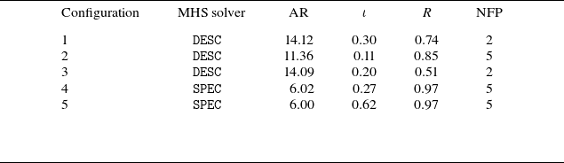
 ι
 R=(max(B)−min(B))/(max(B)+min(B))

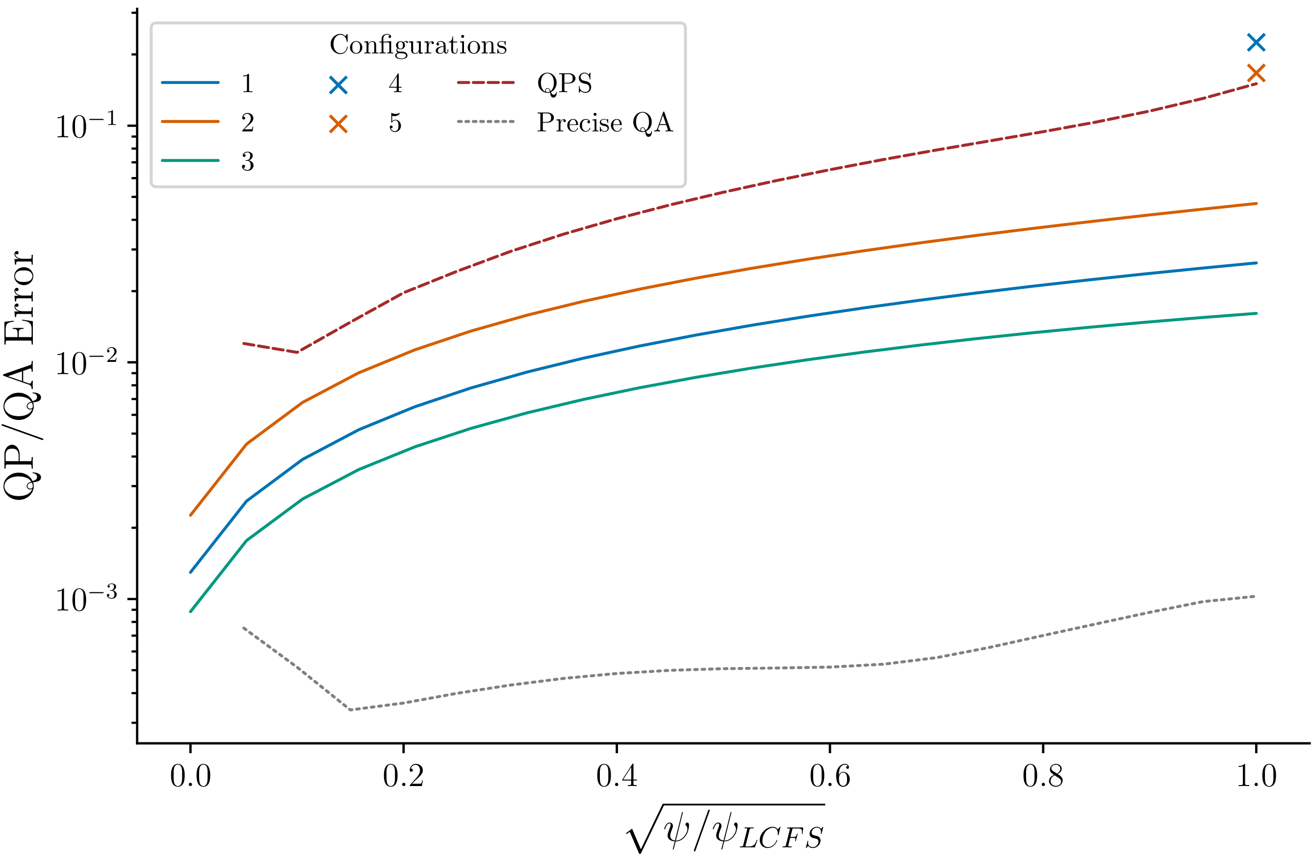

 ϕ<π/2
 κ/ρ
 ϕ
 ϕ>π/2
 κ/ρ

 κ/ρ
 κg

 κ/ρ
 κg
 J∥

 κ/ρ
 κg
 κn

 κg
 κ/ρ

 κg
 κ/ρ


 Open access

