1 Introduction
Poiseuille flow has long served as the archetypal flow for examining near-wall instability, transition and turbulence phenomena (Landahl Reference Landahl1980; Thomson Reference Thomson1887; Butler & Farrell Reference Butler and Farrell1992; Schmid & Henningson Reference Schmid and Henningson2001). This flow embodies much of the fundamental physical features of complex engineering boundary layers without many of the undue complications. Poiseuille flow is ideally suited for examining the fundamental effects of compressibility on wall-bounded shear flows at high Mach numbers. With increasing Mach number, pressure undergoes a profound change in character. At low Mach numbers, hydrodynamic pressure is a Lagrange multiplier (Reddy Reference Reddy1984) with the only function of preserving the divergence-free velocity field. The resulting low Mach number velocity field is solenoidal in character. At higher Mach numbers, pressure is a bona fide thermodynamic state variable and its evolution is governed by energy and state equations. Pressure then exhibits wave behaviour, leading to the emergence of a dilatational (wave-like) component of the velocity field. This leads to profound changes in pressure–velocity interactions which affects flow stability and turbulence. The objective of the present work is to contrast the evolution of small perturbations in Poiseuille flow at high and low Mach numbers. The focus is on understanding the influence of changing pressure–velocity interaction on perturbation evolution at different speeds. The interactions are first examined by performing linear analysis of compressible Poiseuille flow and then the inferences are verified against temporal direct numerical simulations (DNS).
In the literature, linear stability theory employing eigenvalue analysis is generally used to examine modal perturbation growth in fluid flows. Since the focus of this work is on understanding the transient pressure–velocity interaction mechanism and its influence on perturbation growth, we perform non-modal initial value analysis of the linearized governing equations along the lines of rapid distortion theory (RDT) – see Simone, Coleman & Cambon (Reference Simone, Coleman and Cambon1997) and Livescu & Madnia (Reference Livescu and Madnia2004).
In recent years, the present group has been developing insight into the pressure–velocity interactions and perturbation growth in homogeneous shear flows (Bertsch, Suman & Girimaji Reference Bertsch, Suman and Girimaji2012; Lavin et al. Reference Lavin, Girimaji, Suman and Yu2012; Kumar, Bertsch & Girimaji Reference Kumar, Bertsch and Girimaji2014; Kumar et al. Reference Kumar, Bertsch, Venugopal and Girimaji2015; Lee, Venugopal & Girimaji Reference Lee, Venugopal and Girimaji2016). Findings from these studies of homogeneous shear turbulence are invaluable for understanding Poiseuille flow behaviour. The major results from previous studies are now summarized.
-
(i) Using RDT, Lavin et al. (Reference Lavin, Girimaji, Suman and Yu2012) establishes that the evolution of turbulent kinetic energy of an isotropically distributed ensemble of perturbation wave vectors in high Mach number homogeneous shear flow exhibits a three-stage evolution. The three stages are demarcated on the basis of the relative magnitude of shear and acoustic time scales. Thus, the shear–acoustic time scale ratio is established as an important parameter influencing perturbation growth.
-
(ii) In Bertsch et al. (Reference Bertsch, Suman and Girimaji2012), the energy exchange between potential energy (pressure) and dilatational kinetic energy is investigated using RDT. Energy redistribution between different Reynolds stress components is also established.
-
(iii) The influence of wave vector orientation on perturbation growth in compressible homogeneous shear flow is examined using RDT and DNS in Kumar et al. (Reference Kumar, Bertsch and Girimaji2014).
-
(iv) Potential control strategies for inhibiting turbulent kinetic energy growth in shear homogeneous flows at high Mach numbers are examined in Kumar et al. (Reference Kumar, Bertsch, Venugopal and Girimaji2015).
-
(v) The competition between return-to-isotropy and potential–kinetic energy equipartition in anisotropic decaying dilatational turbulence is investigated in Lee et al. (Reference Lee, Venugopal and Girimaji2016) using DNS.
The above studies establish the nature of interactions between pressure and velocity fields in homogeneous turbulence. In Karimi & Girimaji (Reference Karimi and Girimaji2016), linear analysis and DNS are extended to mixing layers. It is shown that the wave-like dilatational velocity field disrupts the Kelvin–Helmholtz rollers inhibiting roll up, instability and thus mixing in high-speed flows. The pressure-released limit of Poiseuille flow is examined in (Xie & Girimaji Reference Xie and Girimaji2014).
The present work examines the effect of compressibility on perturbation growth in compressible Poiseuille flow. One of the key objectives of this work is to investigate the effect of the dilatational field on Tollmien–Schlichting waves which initiate transition to turbulence in many boundary layers of practical importance. The focus of the work is to understand compressibility-induced physical mechanisms that influence perturbation evolution. The principal goal is to explain the transient behaviour in the context of changing pressure–velocity interactions with increasing Mach number. While this insight is important for developing transition and turbulence models, such efforts are deferred to future works. We perform the following studies.
-
(i) Analyse the initial value problem arising from the linearized perturbation equations to compare and contrast the pressure–velocity interactions in incompressible and compressible flows. The role of perturbation mode orientation with respect to the shear plane is examined.
-
(ii) Perform temporally evolving direct numerical simulations of small perturbation growth in compressible Poiseuille flow with a parabolic base field sustained by suitable forcing. The base temperature and pressure fields are determined from the requirement that the parabolic velocity field is a steady state solution of the governing equations. Both adiabatic and isothermal wall boundary conditions are considered. The simulations cover a wide range of Mach and Reynolds numbers.
-
(iii) Use linear analysis and DNS results to develop a clear physical explanation of the pressure–velocity interactions and their effect on the transient evolution of small perturbations in wall-bounded high-speed flows.
The governing equations and linear analysis are presented in § 2. A brief introduction of the numerical approach is given in § 3. The DNS results are presented in § 4. The results and the outcome of linear analysis are used to develop a physical explanation of the underlying pressure–velocity interactions. We close in § 5 with a summary of the salient contributions.
2 Governing equations and linear analysis
The compressible Navier–Stokes equations along with ideal-gas law form the basis of this study:
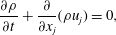 $$\begin{eqnarray}\displaystyle & \displaystyle \frac{\unicode[STIX]{x2202}\unicode[STIX]{x1D70C}}{\unicode[STIX]{x2202}t}+\frac{\unicode[STIX]{x2202}}{\unicode[STIX]{x2202}x_{j}}(\unicode[STIX]{x1D70C}u_{j})=0, & \displaystyle\end{eqnarray}$$
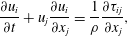 $$\begin{eqnarray}\displaystyle & \displaystyle \frac{\unicode[STIX]{x2202}u_{i}}{\unicode[STIX]{x2202}t}+u_{j}\frac{\unicode[STIX]{x2202}u_{i}}{\unicode[STIX]{x2202}x_{j}}=\frac{1}{\unicode[STIX]{x1D70C}}\frac{\unicode[STIX]{x2202}\unicode[STIX]{x1D70F}_{ij}}{\unicode[STIX]{x2202}x_{j}}, & \displaystyle\end{eqnarray}$$
 $$\begin{eqnarray}\displaystyle & \displaystyle \unicode[STIX]{x1D70C}c_{v}\left(\frac{\unicode[STIX]{x2202}T}{\unicode[STIX]{x2202}t}+u_{j}\frac{\unicode[STIX]{x2202}T}{\unicode[STIX]{x2202}x_{j}}\right)=\frac{\unicode[STIX]{x2202}}{\unicode[STIX]{x2202}x_{j}}\left(k\frac{\unicode[STIX]{x2202}T}{\unicode[STIX]{x2202}x_{j}}\right)+\unicode[STIX]{x1D70F}_{ij}\unicode[STIX]{x1D626}_{ij}, & \displaystyle\end{eqnarray}$$
 $$\begin{eqnarray}\displaystyle & \displaystyle p=\unicode[STIX]{x1D70C}RT, & \displaystyle\end{eqnarray}$$
where
 $\unicode[STIX]{x1D70C}$
is the fluid density,
 $u_{i}$
is velocity component,
 $T$
is temperature,
 $p$
is the gas pressure,
 $\unicode[STIX]{x1D70F}_{ij}$
is the full stress tensor,
 $\unicode[STIX]{x1D626}_{ij}$
is the rate of strain tensor,
 $c_{v}$
is the specific heat at constant volume,
 $k$
is the coefficient of thermal conductivity,
 $R$
is the specific gas constant,
 $x_{i}$
is the spatial coordinate and
 $t$
is time. The rate of strain and stress tensors are given by:
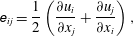 $$\begin{eqnarray}\displaystyle & \displaystyle \unicode[STIX]{x1D626}_{ij}=\frac{1}{2}\left(\frac{\unicode[STIX]{x2202}u_{i}}{\unicode[STIX]{x2202}x_{j}}+\frac{\unicode[STIX]{x2202}u_{j}}{\unicode[STIX]{x2202}x_{i}}\right), & \displaystyle\end{eqnarray}$$
 $$\begin{eqnarray}\displaystyle & \displaystyle \unicode[STIX]{x1D70F}_{ij}=2\unicode[STIX]{x1D707}~\unicode[STIX]{x1D626}_{ij}+\left[{\textstyle \frac{2}{3}}(\unicode[STIX]{x1D706}-\unicode[STIX]{x1D707})\unicode[STIX]{x1D626}_{kk}-p\right]\unicode[STIX]{x1D6FF}_{ij}, & \displaystyle\end{eqnarray}$$
where
 $\unicode[STIX]{x1D707}$
is the coefficient of dynamic viscosity,
 $\unicode[STIX]{x1D706}$
is the coefficient of second viscosity and
 $\unicode[STIX]{x1D6FF}_{ij}$
is the Kronecker delta. We consider a calorically perfect gas and set the Prandtl number (
 $Pr$
) to
 $0.7$
. The specific heat ratio
 $\unicode[STIX]{x1D6FE}$
is
 $1.4$
. The dynamic viscosity is assumed to follow Sutherland’s law (Heiser & Pratt Reference Heiser and Pratt1994):
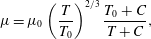 $$\begin{eqnarray}\unicode[STIX]{x1D707}=\unicode[STIX]{x1D707}_{0}\left(\frac{T}{T_{0}}\right)^{2/3}\frac{T_{0}+C}{T+C},\end{eqnarray}$$
where
 $T_{0}$
is the reference temperature which is
 $273.15~\text{K}$
,
 $\unicode[STIX]{x1D707}_{0}$
is the viscosity at reference temperature which is
 $1.716\times 10^{-5}~\text{kg}~\text{m}~\text{s}^{-1}$
and
 $C$
is the Sutherland temperature which is
 $110.4~\text{K}$
. The DNS performed in this study solve the full set of equations. The analysis is however restricted to linearized equations.
2.1 Linear analysis
The objective of the study is to examine small perturbation evolution in a compressible parallel shear flow subject to the above conservation and state equations. The flow and thermodynamic variables are decomposed into base and perturbation fields:
 $$\begin{eqnarray}\unicode[STIX]{x1D70C}=\overline{\unicode[STIX]{x1D70C}}+\unicode[STIX]{x1D70C}^{\prime };\quad u_{i}=\bar{U}_{i}+u_{i}^{\prime };\quad p=\bar{p}+p^{\prime };\quad T=\bar{T}+T^{\prime },\end{eqnarray}$$
where
 $\bar{(\cdot )}$
and
 $(\cdot )^{\prime }$
represent the base/background flow and the perturbation field, respectively. The base flow satisfies the following equations:
 $$\begin{eqnarray}\displaystyle & \displaystyle \frac{\unicode[STIX]{x2202}\bar{\unicode[STIX]{x1D70C}}}{\unicode[STIX]{x2202}t}+\frac{\unicode[STIX]{x2202}\bar{\unicode[STIX]{x1D70C}}\bar{U}_{i}}{\unicode[STIX]{x2202}x_{i}}=0, & \displaystyle\end{eqnarray}$$
 $$\begin{eqnarray}\displaystyle & \displaystyle \frac{\unicode[STIX]{x2202}\bar{U}_{i}}{\unicode[STIX]{x2202}t}+\bar{U}_{j}\frac{\unicode[STIX]{x2202}\bar{U}_{i}}{\unicode[STIX]{x2202}x_{j}}=-\frac{1}{\bar{\unicode[STIX]{x1D70C}}}\frac{\unicode[STIX]{x2202}\bar{p}}{\unicode[STIX]{x2202}x_{i}}+\frac{1}{\bar{\unicode[STIX]{x1D70C}}}\frac{\unicode[STIX]{x2202}}{\unicode[STIX]{x2202}x_{j}}\left[\unicode[STIX]{x1D707}\left(\frac{\unicode[STIX]{x2202}\bar{U}_{i}}{\unicode[STIX]{x2202}x_{j}}+\frac{\unicode[STIX]{x2202}\bar{U}_{j}}{\unicode[STIX]{x2202}x_{i}}\right)\right]+\frac{1}{\bar{\unicode[STIX]{x1D70C}}}\frac{\unicode[STIX]{x2202}}{\unicode[STIX]{x2202}x_{i}}\left[\frac{2}{3}(\unicode[STIX]{x1D706}-\unicode[STIX]{x1D707})\frac{\unicode[STIX]{x2202}\bar{U}_{j}}{\unicode[STIX]{x2202}x_{j}}\right],\qquad & \displaystyle\end{eqnarray}$$
 $$\begin{eqnarray}\displaystyle & \displaystyle \frac{\unicode[STIX]{x2202}\bar{p}}{\unicode[STIX]{x2202}t}+\bar{U}_{j}\frac{\unicode[STIX]{x2202}\bar{p}}{\unicode[STIX]{x2202}x_{j}}=-\bar{p}\unicode[STIX]{x1D6FE}\frac{\unicode[STIX]{x2202}\bar{U}_{k}}{\unicode[STIX]{x2202}x_{k}}+\bar{f}(k)+\bar{g}(\unicode[STIX]{x1D707}), & \displaystyle\end{eqnarray}$$
where
 $\bar{f}(k)$
and
 $\bar{g}(\unicode[STIX]{x1D707})$
denote the effects of heat conduction and viscous transport on the base field, defined as:
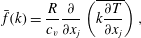 $$\begin{eqnarray}\displaystyle & \displaystyle \bar{f}(k)=\frac{R}{c_{v}}\frac{\unicode[STIX]{x2202}}{\unicode[STIX]{x2202}x_{j}}\left(\overline{k\frac{\unicode[STIX]{x2202}T}{\unicode[STIX]{x2202}x_{j}}}\right), & \displaystyle\end{eqnarray}$$
 $$\begin{eqnarray}\displaystyle & \displaystyle \bar{g}(\unicode[STIX]{x1D707})=\frac{R}{c_{v}}\left[2\overline{\unicode[STIX]{x1D707}\,\unicode[STIX]{x1D626}_{ij}\unicode[STIX]{x1D626}_{ij}}+\frac{2}{3}\overline{(\unicode[STIX]{x1D706}-\unicode[STIX]{x1D707})\unicode[STIX]{x1D626}_{kk}\unicode[STIX]{x1D626}_{kk}}\right]. & \displaystyle\end{eqnarray}$$
2.1.1 Simplifying assumptions for Poiseuille flows
In this work, the base flow is a planar shear flow with parallel streamlines:
 $$\begin{eqnarray}\bar{U}_{i}=(\bar{U}_{1}(x_{2}),0,0)\text{ leading to }\unicode[STIX]{x2202}\bar{U}_{i}/\unicode[STIX]{x2202}x_{i}=0.\end{eqnarray}$$
Here,
 $x_{1}$
is defined as the streamwise direction,
 $x_{2}$
is the wall-normal direction and
 $x_{3}$
is the spanwise direction. In numerical simulations, this velocity field is sustained using appropriate forcing (Xie & Girimaji Reference Xie and Girimaji2014). Due to body-force type of forcing, the background density and pressure fields are nearly spatially invariant to linear order. Thus for the purpose of analysis we assume
 $$\begin{eqnarray}\bar{\unicode[STIX]{x1D70C}}(\boldsymbol{x})\approx \text{Const.};\quad \bar{p}(\boldsymbol{x})\approx \text{Const.}\end{eqnarray}$$
A perturbation is introduced into the background field and its subsequent evolution is the subject of the numerical simulations and linear analysis. The nonlinear effects and variations in fluid properties such as viscosity and heat conductivity are neglected in the analysis:
 $$\begin{eqnarray}\unicode[STIX]{x1D707}(\boldsymbol{x})\approx \text{Const.};\quad k(\boldsymbol{x})\approx \text{Const.}\end{eqnarray}$$
In the numerical simulations, however,
 $\bar{\unicode[STIX]{x1D70C}}$
,
 $\bar{p}$
,
 $\unicode[STIX]{x1D707}$
and
 $k$
vary according to the governing equations.
2.1.2 Perturbation equations for Poiseuille flows
By subtracting base flow equations from those of instantaneous flow, the linearized perturbation evolution equations are derived:
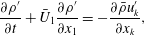 $$\begin{eqnarray}\displaystyle & \displaystyle \frac{\unicode[STIX]{x2202}\unicode[STIX]{x1D70C}^{\prime }}{\unicode[STIX]{x2202}t}+\bar{U}_{1}\frac{\unicode[STIX]{x2202}\unicode[STIX]{x1D70C}^{\prime }}{\unicode[STIX]{x2202}x_{1}}=-\frac{\unicode[STIX]{x2202}\bar{\unicode[STIX]{x1D70C}}u_{k}^{\prime }}{\unicode[STIX]{x2202}x_{k}}, & \displaystyle\end{eqnarray}$$
 $$\begin{eqnarray}\displaystyle & \displaystyle \frac{\unicode[STIX]{x2202}u_{1}^{\prime }}{\unicode[STIX]{x2202}t}+\bar{U}_{1}\frac{\unicode[STIX]{x2202}u_{1}^{\prime }}{\unicode[STIX]{x2202}x_{1}}=-\frac{1}{\bar{\unicode[STIX]{x1D70C}}}\frac{\unicode[STIX]{x2202}p^{\prime }}{\unicode[STIX]{x2202}x_{1}}-u_{2}^{\prime }\frac{\unicode[STIX]{x2202}\bar{U}_{1}}{\unicode[STIX]{x2202}x_{2}}+\frac{\unicode[STIX]{x1D707}}{\bar{\unicode[STIX]{x1D70C}}}\frac{\unicode[STIX]{x2202}}{\unicode[STIX]{x2202}x_{j}}\left(\frac{\unicode[STIX]{x2202}u_{1}^{\prime }}{\unicode[STIX]{x2202}x_{j}}+\frac{\unicode[STIX]{x2202}u_{j}^{\prime }}{\unicode[STIX]{x2202}x_{1}}\right)+\frac{2(\unicode[STIX]{x1D706}-\unicode[STIX]{x1D707})}{3\bar{\unicode[STIX]{x1D70C}}}\frac{\unicode[STIX]{x2202}}{\unicode[STIX]{x2202}x_{1}}\left(\frac{\unicode[STIX]{x2202}u_{j}^{\prime }}{\unicode[STIX]{x2202}x_{j}}\right), & \displaystyle \nonumber\\ \displaystyle & & \displaystyle\end{eqnarray}$$
 $$\begin{eqnarray}\displaystyle & \displaystyle \frac{\unicode[STIX]{x2202}u_{2}^{\prime }}{\unicode[STIX]{x2202}t}+\bar{U}_{1}\frac{\unicode[STIX]{x2202}u_{2}^{\prime }}{\unicode[STIX]{x2202}x_{1}}=-\frac{1}{\bar{\unicode[STIX]{x1D70C}}}\frac{\unicode[STIX]{x2202}p^{\prime }}{\unicode[STIX]{x2202}x_{2}}+\frac{\unicode[STIX]{x1D707}}{\bar{\unicode[STIX]{x1D70C}}}\frac{\unicode[STIX]{x2202}}{\unicode[STIX]{x2202}x_{j}}\left(\frac{\unicode[STIX]{x2202}u_{2}^{\prime }}{\unicode[STIX]{x2202}x_{j}}+\frac{\unicode[STIX]{x2202}u_{j}^{\prime }}{\unicode[STIX]{x2202}x_{2}}\right)+\frac{2(\unicode[STIX]{x1D706}-\unicode[STIX]{x1D707})}{3\bar{\unicode[STIX]{x1D70C}}}\frac{\unicode[STIX]{x2202}}{\unicode[STIX]{x2202}x_{2}}\left(\frac{\unicode[STIX]{x2202}u_{j}^{\prime }}{\unicode[STIX]{x2202}x_{j}}\right), & \displaystyle\end{eqnarray}$$
 $$\begin{eqnarray}\displaystyle & \displaystyle \frac{\unicode[STIX]{x2202}u_{3}^{\prime }}{\unicode[STIX]{x2202}t}+\bar{U}_{1}\frac{\unicode[STIX]{x2202}u_{3}^{\prime }}{\unicode[STIX]{x2202}x_{1}}=-\frac{1}{\bar{\unicode[STIX]{x1D70C}}}\frac{\unicode[STIX]{x2202}p^{\prime }}{\unicode[STIX]{x2202}x_{3}}+\frac{\unicode[STIX]{x1D707}}{\bar{\unicode[STIX]{x1D70C}}}\frac{\unicode[STIX]{x2202}}{\unicode[STIX]{x2202}x_{j}}\left(\frac{\unicode[STIX]{x2202}u_{3}^{\prime }}{\unicode[STIX]{x2202}x_{j}}+\frac{\unicode[STIX]{x2202}u_{j}^{\prime }}{\unicode[STIX]{x2202}x_{3}}\right)+\frac{2(\unicode[STIX]{x1D706}-\unicode[STIX]{x1D707})}{3\bar{\unicode[STIX]{x1D70C}}}\frac{\unicode[STIX]{x2202}}{\unicode[STIX]{x2202}x_{3}}\left(\frac{\unicode[STIX]{x2202}u_{j}^{\prime }}{\unicode[STIX]{x2202}x_{j}}\right), & \displaystyle\end{eqnarray}$$
 $$\begin{eqnarray}\displaystyle & \displaystyle \frac{\unicode[STIX]{x2202}p^{\prime }}{\unicode[STIX]{x2202}t}+\bar{U}_{1}\frac{\unicode[STIX]{x2202}p^{\prime }}{\unicode[STIX]{x2202}x_{1}}=-\bar{p}\unicode[STIX]{x1D6FE}\left(\frac{\unicode[STIX]{x2202}u_{k}^{\prime }}{\unicode[STIX]{x2202}x_{k}}\right)+f^{\prime }(k)+g^{\prime }(\unicode[STIX]{x1D707}), & \displaystyle\end{eqnarray}$$
where the functions
 $f^{\prime }(k)$
and
 $g^{\prime }(\unicode[STIX]{x1D707})$
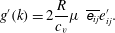
represents the linear effects of heat conduction and viscous transport on the perturbation field. For the simplified case considered in this analysis, these function are given by
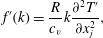 $$\begin{eqnarray}\displaystyle & \displaystyle f^{\prime }(k)=\frac{R}{c_{v}}k\frac{\unicode[STIX]{x2202}^{2}T^{\prime }}{\unicode[STIX]{x2202}x_{j}^{2}}, & \displaystyle\end{eqnarray}$$
 $$\begin{eqnarray}\displaystyle & \displaystyle g^{\prime }(k)=2\frac{R}{c_{v}}\unicode[STIX]{x1D707}~\overline{\unicode[STIX]{x1D626}_{ij}}e_{ij}^{\prime }. & \displaystyle\end{eqnarray}$$
However, for the more general case that
 $k$
and
 $\unicode[STIX]{x1D707}$
vary with temperature, the reader is referred to Mack (Reference Mack1984).
The growth in the perturbation kinetic energy is due to the production term:
 $-u_{2}^{\prime }(\unicode[STIX]{x2202}\bar{U}_{1}/\unicode[STIX]{x2202}x_{2})$
on the right-hand side of (2.18). It is also important to examine perturbation vorticity evolution. For the sake of comparison between baroclinic and other compressibility effects, we temporarily include the background density variation. From the velocity field, the linearized vorticity perturbation equations can be obtained:
 $$\begin{eqnarray}\displaystyle \frac{\unicode[STIX]{x2202}\unicode[STIX]{x1D714}_{1}^{\prime }}{\unicode[STIX]{x2202}t}+\bar{U}_{1}\frac{\unicode[STIX]{x2202}\unicode[STIX]{x1D714}_{1}^{\prime }}{\unicode[STIX]{x2202}x_{1}} & = & \displaystyle \frac{1}{\bar{\unicode[STIX]{x1D70C}}^{2}}\frac{\unicode[STIX]{x2202}\bar{\unicode[STIX]{x1D70C}}}{\unicode[STIX]{x2202}x_{2}}\frac{\unicode[STIX]{x2202}p^{\prime }}{\unicode[STIX]{x2202}x_{3}}-\frac{\unicode[STIX]{x2202}\bar{U}_{1}}{\unicode[STIX]{x2202}x_{2}}\frac{\unicode[STIX]{x2202}u_{3}^{\prime }}{\unicode[STIX]{x2202}x_{1}}-\frac{\unicode[STIX]{x1D707}}{\bar{\unicode[STIX]{x1D70C}}^{2}}\frac{\unicode[STIX]{x2202}\bar{\unicode[STIX]{x1D70C}}}{\unicode[STIX]{x2202}x_{2}}\bigg(\frac{\unicode[STIX]{x2202}^{2}u_{3}^{\prime }}{\unicode[STIX]{x2202}^{2}x_{k}}-\frac{1}{9}\frac{\unicode[STIX]{x2202}^{2}u_{k}^{\prime }}{\unicode[STIX]{x2202}x_{3}\unicode[STIX]{x2202}x_{k}}\bigg)\nonumber\\ \displaystyle & & \displaystyle +\,\frac{\unicode[STIX]{x1D707}}{\bar{\unicode[STIX]{x1D70C}}}\left(\frac{\unicode[STIX]{x2202}^{3}u_{3}^{\prime }}{\unicode[STIX]{x2202}^{2}x_{k}\unicode[STIX]{x2202}x_{2}}-\frac{\unicode[STIX]{x2202}^{3}u_{2}^{\prime }}{\unicode[STIX]{x2202}^{2}x_{k}\unicode[STIX]{x2202}x_{3}}\right),\end{eqnarray}$$
 $$\begin{eqnarray}\displaystyle \frac{\unicode[STIX]{x2202}\unicode[STIX]{x1D714}_{2}^{\prime }}{\unicode[STIX]{x2202}t}+\bar{U}_{1}\frac{\unicode[STIX]{x2202}\unicode[STIX]{x1D714}_{2}^{\prime }}{\unicode[STIX]{x2202}x_{1}} & = & \displaystyle -\frac{\unicode[STIX]{x2202}\bar{U}_{1}}{\unicode[STIX]{x2202}x_{2}}\frac{\unicode[STIX]{x2202}u_{2}^{\prime }}{\unicode[STIX]{x2202}x_{3}}+\frac{\unicode[STIX]{x1D707}}{\bar{\unicode[STIX]{x1D70C}}}\left(\frac{\unicode[STIX]{x2202}^{3}u_{1}^{\prime }}{\unicode[STIX]{x2202}^{2}x_{k}\unicode[STIX]{x2202}x_{3}}-\frac{\unicode[STIX]{x2202}^{3}u_{3}^{\prime }}{\unicode[STIX]{x2202}^{2}x_{k}\unicode[STIX]{x2202}x_{1}}\right),\end{eqnarray}$$
 $$\begin{eqnarray}\displaystyle \frac{\unicode[STIX]{x2202}\unicode[STIX]{x1D714}_{3}^{\prime }}{\unicode[STIX]{x2202}t}+\bar{U}_{1}\frac{\unicode[STIX]{x2202}\unicode[STIX]{x1D714}_{3}^{\prime }}{\unicode[STIX]{x2202}x_{1}} & = & \displaystyle \frac{1}{\bar{\unicode[STIX]{x1D70C}}^{2}}\frac{\unicode[STIX]{x2202}\bar{\unicode[STIX]{x1D70C}}}{\unicode[STIX]{x2202}x_{2}}\frac{\unicode[STIX]{x2202}p^{\prime }}{\unicode[STIX]{x2202}x_{1}}-\frac{\unicode[STIX]{x2202}\bar{U}_{1}}{\unicode[STIX]{x2202}x_{2}}\left(\frac{\unicode[STIX]{x2202}u_{1}^{\prime }}{\unicode[STIX]{x2202}x_{1}}+\frac{\unicode[STIX]{x2202}u_{2}^{\prime }}{\unicode[STIX]{x2202}x_{2}}\right)-\frac{\unicode[STIX]{x1D707}}{\bar{\unicode[STIX]{x1D70C}}^{2}}\frac{\unicode[STIX]{x2202}\bar{\unicode[STIX]{x1D70C}}}{\unicode[STIX]{x2202}x_{2}}\left(\frac{\unicode[STIX]{x2202}^{2}u_{1}^{\prime }}{\unicode[STIX]{x2202}^{2}x_{k}}-\frac{1}{9}\frac{\unicode[STIX]{x2202}^{2}u_{k}^{\prime }}{\unicode[STIX]{x2202}x_{1}\unicode[STIX]{x2202}x_{k}}\right)\nonumber\\ \displaystyle & & \displaystyle +\,\frac{\unicode[STIX]{x1D707}}{\bar{\unicode[STIX]{x1D70C}}}\left(\frac{\unicode[STIX]{x2202}^{3}u_{2}^{\prime }}{\unicode[STIX]{x2202}^{2}x_{k}\unicode[STIX]{x2202}x_{1}}-\frac{\unicode[STIX]{x2202}^{3}u_{1}^{\prime }}{\unicode[STIX]{x2202}^{2}x_{k}\unicode[STIX]{x2202}x_{2}}\right)+u_{2}^{\prime }\frac{\unicode[STIX]{x2202}^{2}\bar{U}_{1}}{\unicode[STIX]{x2202}^{2}x_{2}}.\end{eqnarray}$$
Among the three components, the spanwise vorticity perturbation (
 $\unicode[STIX]{x1D714}_{3}^{\prime }$
) is the most relevant for shear flow instability investigation as it is central to Tollmien–Schlichting (TS) wave formation. In spanwise vorticity perturbation equation (2.26), multiple mechanisms can be identified. On the right-hand side of (2.26), the first term
 $(\unicode[STIX]{x2202}\bar{\unicode[STIX]{x1D70C}}/\unicode[STIX]{x2202}x_{2})(\unicode[STIX]{x2202}p^{\prime }/\unicode[STIX]{x2202}x_{1})/\bar{\unicode[STIX]{x1D70C}}^{2}$
represents the baroclinic effect, the second term
 $(\unicode[STIX]{x2202}\bar{U}_{1}/\unicode[STIX]{x2202}x_{2})\left(\unicode[STIX]{x2202}u_{1}^{\prime }/\unicode[STIX]{x2202}x_{1}+\unicode[STIX]{x2202}u_{2}^{\prime }/\unicode[STIX]{x2202}x_{2}\right)$
represents compressible vortex production (CVP), the third and fourth terms denote viscous effects and finally the last term
 $u_{2}^{\prime }(\unicode[STIX]{x2202}^{2}\bar{U}_{1}/\unicode[STIX]{x2202}^{2}x_{2})$
is the second derivative effect.
Inspection of the transport equations reveals that instability of shear flows manifest via two critical terms:
 $u_{2}^{\prime }(\unicode[STIX]{x2202}\bar{U}_{1}/\unicode[STIX]{x2202}x_{2})$
in the velocity equation (2.19) and
 $u_{2}^{\prime }(\unicode[STIX]{x2202}^{2}\bar{U}_{1}/\unicode[STIX]{x2202}^{2}x_{2})$
in the vorticity equation (2.26). Clearly, the evolution of normal perturbation (
 $u_{2}^{\prime }$
) plays a major role in determining the instability growth characteristics in both incompressible and compressible shear flows. Thus, the first key challenge is to establish how the change in character of pressure affects the evolution of
 $u_{2}^{\prime }$
. Considering the spanwise vorticity equation, it is evident that the compressibility effects also manifest via the baroclinic and CVP terms. Then, the second challenge is to examine the balance between the second derivative and the compressibility effects.
2.2 Pressure–velocity interaction in compressible flows
To examine the pressure–velocity interactions in an arbitrary planar shear flow, we temporarily suppress the viscous terms. The inviscid perturbation equations are:
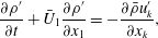 $$\begin{eqnarray}\displaystyle & \displaystyle \frac{\unicode[STIX]{x2202}\unicode[STIX]{x1D70C}^{\prime }}{\unicode[STIX]{x2202}t}+\bar{U}_{1}\frac{\unicode[STIX]{x2202}\unicode[STIX]{x1D70C}^{\prime }}{\unicode[STIX]{x2202}x_{1}}=-\frac{\unicode[STIX]{x2202}\bar{\unicode[STIX]{x1D70C}}u_{k}^{\prime }}{\unicode[STIX]{x2202}x_{k}}, & \displaystyle\end{eqnarray}$$
 $$\begin{eqnarray}\displaystyle & \displaystyle \frac{\unicode[STIX]{x2202}u_{1}^{\prime }}{\unicode[STIX]{x2202}t}+\bar{U_{1}}\frac{\unicode[STIX]{x2202}u_{1}^{\prime }}{\unicode[STIX]{x2202}x_{1}}=-\frac{1}{\bar{\unicode[STIX]{x1D70C}}}\frac{\unicode[STIX]{x2202}p^{\prime }}{\unicode[STIX]{x2202}x_{1}}-u_{2}^{\prime }\frac{\unicode[STIX]{x2202}\bar{U}_{1}}{\unicode[STIX]{x2202}x_{2}}, & \displaystyle\end{eqnarray}$$
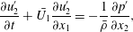 $$\begin{eqnarray}\displaystyle & \displaystyle \frac{\unicode[STIX]{x2202}u_{2}^{\prime }}{\unicode[STIX]{x2202}t}+\bar{U_{1}}\frac{\unicode[STIX]{x2202}u_{2}^{\prime }}{\unicode[STIX]{x2202}x_{1}}=-\frac{1}{\bar{\unicode[STIX]{x1D70C}}}\frac{\unicode[STIX]{x2202}p^{\prime }}{\unicode[STIX]{x2202}x_{2}}, & \displaystyle\end{eqnarray}$$
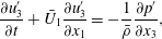 $$\begin{eqnarray}\displaystyle & \displaystyle \frac{\unicode[STIX]{x2202}u_{3}^{\prime }}{\unicode[STIX]{x2202}t}+\bar{U_{1}}\frac{\unicode[STIX]{x2202}u_{3}^{\prime }}{\unicode[STIX]{x2202}x_{1}}=-\frac{1}{\bar{\unicode[STIX]{x1D70C}}}\frac{\unicode[STIX]{x2202}p^{\prime }}{\unicode[STIX]{x2202}x_{3}}, & \displaystyle\end{eqnarray}$$
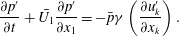 $$\begin{eqnarray}\displaystyle & \displaystyle \frac{\unicode[STIX]{x2202}p^{\prime }}{\unicode[STIX]{x2202}t}+\bar{U_{1}}\frac{\unicode[STIX]{x2202}p^{\prime }}{\unicode[STIX]{x2202}x_{1}}=-\bar{p}\unicode[STIX]{x1D6FE}\left(\frac{\unicode[STIX]{x2202}u_{k}^{\prime }}{\unicode[STIX]{x2202}x_{k}}\right). & \displaystyle\end{eqnarray}$$
To facilitate further analysis, we apply the Howarth–Dorodnitsyn transformation (Howarth Reference Howarth1948). The flow evolution is now described in a coordinate moving with the background convective velocity:
 $$\begin{eqnarray}X_{1}=x_{1}-\int _{0}^{t}U_{1}(x_{2})\,\text{d}\unicode[STIX]{x1D709},\quad X_{2}=x_{2},\quad X_{3}=x_{3},\quad t=t.\end{eqnarray}$$
The perturbation equations (2.17)–(2.21) can be rewritten in the new frame as follows:
 $$\begin{eqnarray}\displaystyle & \displaystyle \frac{\text{d}\unicode[STIX]{x1D70C}^{\prime }}{\text{d}t}=-\frac{\unicode[STIX]{x2202}\bar{\unicode[STIX]{x1D70C}}u_{1}^{\prime }}{\unicode[STIX]{x2202}X_{1}}+\frac{\unicode[STIX]{x2202}\bar{\unicode[STIX]{x1D70C}}u_{2}^{\prime }}{\unicode[STIX]{x2202}X_{2}}-\frac{\unicode[STIX]{x2202}\bar{\unicode[STIX]{x1D70C}}u_{2}^{\prime }}{\unicode[STIX]{x2202}X_{1}}\int _{0}^{t}\frac{\unicode[STIX]{x2202}\bar{U}_{1}}{\unicode[STIX]{x2202}x_{2}}\,\text{d}\unicode[STIX]{x1D709}+\frac{\unicode[STIX]{x2202}\bar{\unicode[STIX]{x1D70C}}u_{3}^{\prime }}{\unicode[STIX]{x2202}X_{3}}, & \displaystyle\end{eqnarray}$$
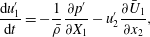 $$\begin{eqnarray}\displaystyle & \displaystyle \frac{\text{d}u_{1}^{\prime }}{\text{d}t}=-\frac{1}{\bar{\unicode[STIX]{x1D70C}}}\frac{\unicode[STIX]{x2202}p^{\prime }}{\unicode[STIX]{x2202}X_{1}}-u_{2}^{\prime }\frac{\unicode[STIX]{x2202}\bar{U}_{1}}{\unicode[STIX]{x2202}x_{2}}, & \displaystyle\end{eqnarray}$$
 $$\begin{eqnarray}\displaystyle & \displaystyle \frac{\text{d}u_{2}^{\prime }}{\text{d}t}=-\frac{1}{\bar{\unicode[STIX]{x1D70C}}}\frac{\unicode[STIX]{x2202}p^{\prime }}{\unicode[STIX]{x2202}X_{2}}+\frac{1}{\bar{\unicode[STIX]{x1D70C}}}\frac{\unicode[STIX]{x2202}p^{\prime }}{\unicode[STIX]{x2202}X_{1}}\int _{0}^{t}\frac{\unicode[STIX]{x2202}\bar{U}_{1}}{\unicode[STIX]{x2202}x_{2}}\,\text{d}\unicode[STIX]{x1D709}, & \displaystyle\end{eqnarray}$$
 $$\begin{eqnarray}\displaystyle & \displaystyle \frac{\text{d}u_{3}^{\prime }}{\text{d}t}=-\frac{1}{\bar{\unicode[STIX]{x1D70C}}}\frac{\unicode[STIX]{x2202}p^{\prime }}{\unicode[STIX]{x2202}X_{3}}, & \displaystyle\end{eqnarray}$$
 $$\begin{eqnarray}\displaystyle & \displaystyle \frac{\text{d}p^{\prime }}{\text{d}t}=-\bar{p}\unicode[STIX]{x1D6FE}\left(\frac{\unicode[STIX]{x2202}u_{1}^{\prime }}{\unicode[STIX]{x2202}X_{1}}+\frac{\unicode[STIX]{x2202}u_{2}^{\prime }}{\unicode[STIX]{x2202}X_{2}}-\frac{\unicode[STIX]{x2202}u_{2}^{\prime }}{\unicode[STIX]{x2202}X_{1}}\int _{0}^{t}\frac{\unicode[STIX]{x2202}\bar{U}_{1}}{\unicode[STIX]{x2202}x_{2}}\,\text{d}\unicode[STIX]{x1D709}+\frac{\unicode[STIX]{x2202}u_{3}^{\prime }}{\unicode[STIX]{x2202}X_{3}}\right). & \displaystyle\end{eqnarray}$$
Without further loss of generality, we will consider perturbation modes that are periodic in
 $X_{1}$
and
 $X_{3}$
with an arbitrary initial profile in the
 $X_{2}$
direction:
 $$\begin{eqnarray}\displaystyle u_{j}^{\prime }=\hat{u} _{j}(X_{2},t)\text{e}^{\text{i}(\unicode[STIX]{x1D705}_{1}X_{1}+\unicode[STIX]{x1D705}_{3}X_{3})};\quad p^{\prime }=\hat{p}~(X_{2},t)\text{e}^{\text{i}(\unicode[STIX]{x1D705}_{1}X_{1}+\unicode[STIX]{x1D705}_{3}X_{3})}, & & \displaystyle\end{eqnarray}$$
where
 $\unicode[STIX]{x1D705}_{1}$
and
 $\unicode[STIX]{x1D705}_{3}$
are the initial perturbation wavenumbers in the streamwise and spanwise directions,
 $\text{i}=\sqrt{-1}$
denotes the unit imaginary number and
 $(\hat{\cdot })$
denotes the amplitude of the corresponding perturbation mode. The amplitude is a function of time and normal coordinate. By substituting (2.38) into (2.34)–(2.37), evolution equations of the Fourier amplitude of the perturbation field can be obtained:
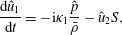 $$\begin{eqnarray}\displaystyle & \displaystyle \frac{\text{d}\hat{u} _{1}}{\text{d}t}=-\text{i}\unicode[STIX]{x1D705}_{1}\frac{\hat{p}}{\bar{\unicode[STIX]{x1D70C}}}-\hat{u} _{2}S, & \displaystyle\end{eqnarray}$$
 $$\begin{eqnarray}\displaystyle & \displaystyle \frac{\text{d}\hat{u} _{2}}{\text{d}t}=-\frac{1}{\bar{\unicode[STIX]{x1D70C}}}\frac{\unicode[STIX]{x2202}\hat{p}}{\unicode[STIX]{x2202}X_{2}}+\text{i}\unicode[STIX]{x1D705}_{1}\frac{\hat{p}}{\bar{\unicode[STIX]{x1D70C}}}\int _{0}^{t}S\,\text{d}\unicode[STIX]{x1D709}, & \displaystyle\end{eqnarray}$$
 $$\begin{eqnarray}\displaystyle & \displaystyle \frac{\text{d}\hat{u} _{3}}{\text{d}t}=-\text{i}\unicode[STIX]{x1D705}_{3}\frac{\hat{p}}{\bar{\unicode[STIX]{x1D70C}}}, & \displaystyle\end{eqnarray}$$
 $$\begin{eqnarray}\displaystyle & \displaystyle \frac{\text{d}\hat{p}}{\text{d}t}=-\unicode[STIX]{x1D6FE}\bar{p}\left[\text{i}\unicode[STIX]{x1D705}_{1}\hat{u} _{1}+\frac{\unicode[STIX]{x2202}\hat{u} _{2}}{\unicode[STIX]{x2202}X_{2}}-\text{i}\unicode[STIX]{x1D705}_{1}\hat{u} _{2}\int _{0}^{t}S\,\text{d}\unicode[STIX]{x1D709}+\text{i}\unicode[STIX]{x1D705}_{3}\hat{u} _{3}\right], & \displaystyle\end{eqnarray}$$
where the background shear in the normal direction,
 $S(x_{2})$
or
 $S$
, is given by
 $$\begin{eqnarray}S=\frac{\unicode[STIX]{x2202}U_{1}}{\unicode[STIX]{x2202}X_{2}}.\end{eqnarray}$$
Equations (2.39)–(2.42) constitute the initial value problem of interest. It is established in previous works on homogeneous shear flows (Livescu & Madnia Reference Livescu and Madnia2004; Kumar et al.
Reference Kumar, Bertsch and Girimaji2014) that dilatational velocity is generated on the shear plane. Dilatational velocity represents a large fraction of the normal perturbation (
 $u_{2}^{\prime }$
) and a small portion of the streamwise component (
 $u_{1}^{\prime }$
). Many of the compressibility effects can be understood by examining the pressure–velocity (
 $p^{\prime }$
–
 $u_{2}^{\prime }$
) interactions at different speed regimes.
To non-dimensionalize the perturbation equations (2.39)–(2.42), we introduce dimensionless time and space coordinates:
 $$\begin{eqnarray}t^{\ast }=St;\quad x_{i}^{\ast }=\unicode[STIX]{x1D705}x_{i},\end{eqnarray}$$
where
 $\unicode[STIX]{x1D705}=|\unicode[STIX]{x1D73F}(0)|=\sqrt{\unicode[STIX]{x1D705}_{1}^{2}+\unicode[STIX]{x1D705}_{3}^{2}}$
is the initial value of the wavenumber magnitude. Equation (2.42) in the non-dimensionalized temporal and spatial coordinates defined in (2.44) can be rewritten as
 $$\begin{eqnarray}\frac{S^{2}}{\bar{a}^{2}\unicode[STIX]{x1D705}^{2}}\frac{\unicode[STIX]{x2202}^{2}\hat{p}}{\unicode[STIX]{x2202}{t^{\ast }}^{2}}=\frac{\unicode[STIX]{x2202}^{2}\hat{p}}{\unicode[STIX]{x2202}x_{2}^{\ast }}-\hat{p}+\left[\text{i}\left(\frac{\unicode[STIX]{x1D705}_{1}}{\unicode[STIX]{x1D705}}\right)\frac{\unicode[STIX]{x2202}S^{\ast }}{\unicode[STIX]{x2202}x_{2}^{\ast }}+\left(\frac{\unicode[STIX]{x1D705}_{1}}{\unicode[STIX]{x1D705}}\right)^{2}{S^{\ast }}^{2}\right]\hat{p}+2\text{i}\left(\frac{\unicode[STIX]{x1D705}_{1}}{\unicode[STIX]{x1D705}}\right)\frac{\bar{\unicode[STIX]{x1D70C}}}{\unicode[STIX]{x1D705}}\hat{u} _{2}S,\end{eqnarray}$$
where
 $\bar{a}=\sqrt{\unicode[STIX]{x1D6FE}\bar{p}/\bar{\unicode[STIX]{x1D70C}}}$
is the speed of sound in the background flow and
 $S^{\ast }=\int _{0}^{t}S\,\text{d}\unicode[STIX]{x1D709}$
.
Definition of an obliqueness angle based on the initial orientation.
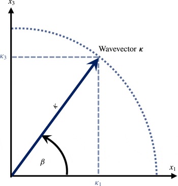
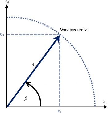
To identify the role of perturbation orientation in the evolution of compressible Poiseuille flow, we introduce two parameters. Firstly, referring to figure 1, the obliqueness angle
 $\unicode[STIX]{x1D6FD}$
is defined as the angle between wave vector
 $\unicode[STIX]{x1D73F}$
and the streamwise coordinate
 $x_{1}$
, given by
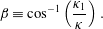 $$\begin{eqnarray}\unicode[STIX]{x1D6FD}\equiv \cos ^{-1}\left(\frac{\unicode[STIX]{x1D705}_{1}}{\unicode[STIX]{x1D705}}\right).\end{eqnarray}$$
Secondly, the effect of compressibility on flow stability is characterized by gradient Mach number,
 $M_{g}$
, defined by (Sarkar Reference Sarkar1995):
 $$\begin{eqnarray}M_{g}\equiv \frac{Sl}{\bar{a}}=\frac{S}{\bar{a}\unicode[STIX]{x1D705}}.\end{eqnarray}$$
Now (2.45) can be written in a form wherein the effects of Mach number and obliqueness can be easily identified:
 $$\begin{eqnarray}M_{g}^{2}\frac{\unicode[STIX]{x2202}^{2}\hat{p}}{\unicode[STIX]{x2202}{t^{\ast }}^{2}}=\frac{\unicode[STIX]{x2202}^{2}\hat{p}}{\unicode[STIX]{x2202}x_{2}^{\ast }}-\hat{p}+\left[\text{i}\frac{\unicode[STIX]{x2202}S^{\ast }}{\unicode[STIX]{x2202}x_{2}^{\ast }}\cos \unicode[STIX]{x1D6FD}+{S^{\ast }}^{2}\cos ^{2}\unicode[STIX]{x1D6FD}\right]\hat{p}+2\text{i}\frac{\bar{\unicode[STIX]{x1D70C}}}{\unicode[STIX]{x1D705}}\hat{u} _{2}S\cos \unicode[STIX]{x1D6FD}.\end{eqnarray}$$
For the sake of convenience, the following normalizations for pressure and velocity amplitude are suggested by:
 $$\begin{eqnarray}\displaystyle \hat{u} _{i}^{\ast }=\hat{u} _{i}/\bar{a};\quad \hat{p}^{\ast }=\hat{p}/\bar{p}. & & \displaystyle\end{eqnarray}$$
These definitions and further mathematical manipulation of equations (2.39)–(2.42) lead to the following hyperbolic equation for pressure:
 $$\begin{eqnarray}M_{g}^{2}\frac{\unicode[STIX]{x2202}^{2}\hat{p}^{\ast }}{\unicode[STIX]{x2202}{t^{\ast }}^{2}}=\frac{\unicode[STIX]{x2202}^{2}\hat{p}^{\ast }}{\unicode[STIX]{x2202}x_{2}^{\ast }}-\hat{p}^{\ast }+\left[\text{i}\frac{\unicode[STIX]{x2202}S^{\ast }}{\unicode[STIX]{x2202}x_{2}^{\ast }}\cos \unicode[STIX]{x1D6FD}+{S^{\ast }}^{2}\cos ^{2}\unicode[STIX]{x1D6FD}\right]\hat{p}^{\ast }+2\text{i}\unicode[STIX]{x1D6FE}\hat{u} _{2}^{\ast }M_{g}\cos \unicode[STIX]{x1D6FD}.\end{eqnarray}$$
Similarly, the velocity perturbation evolution can be described by an inhomogeneous wave equation. Differentiating (2.40) twice with respect to time yields
 $$\begin{eqnarray}M_{g}^{2}\frac{\unicode[STIX]{x2202}^{2}\hat{u} _{2}^{\ast }}{\unicode[STIX]{x2202}{t^{\ast }}^{2}}=\frac{\unicode[STIX]{x2202}^{2}\hat{u} _{2}^{\ast }}{\unicode[STIX]{x2202}{x_{2}^{\ast }}^{2}}-\left[(\hat{u} _{1}^{\ast }-\hat{u} _{2}^{\ast }S^{\ast })\cos ^{2}\unicode[STIX]{x1D6FD}+\left(\hat{u} _{3}^{\ast }\sin \unicode[STIX]{x1D6FD}+\text{i}\frac{\unicode[STIX]{x2202}\hat{u} _{2}^{\ast }}{\unicode[STIX]{x2202}x_{2}^{\ast }}\right)\cos \unicode[STIX]{x1D6FD}\right]S^{\ast }-\text{i}\frac{\hat{p}^{\ast }}{\unicode[STIX]{x1D6FE}}M_{g}\cos \unicode[STIX]{x1D6FD},\end{eqnarray}$$
where
 $S^{\ast }=S^{\ast }(X_{2},t)=\int _{0}^{t}S(X_{2})\,\text{d}\unicode[STIX]{x1D709}$
. Note that equations (2.50)–(2.51) describe the evolution of perturbation in any general planar compressible shear flow. These equations are not amenable to straightforward analytical solution. Instead, we seek valuable insight based on the form of the governing equations and by examination of the behaviour at certain asymptotic limits in a compressible Poiseuille flow.
First and foremost, based on the definition of the relevant Mach number
 $M_{g}$
(2.47), three distinct regions in high-speed Poiseuille flow can be identified. In general, the shear in the near-wall regions is much higher than in the central region. In low-speed flows, the gradient Mach numbers throughout the channel will be less than unity and the flow field will be solenoidal in character. However, at higher speeds, the gradient Mach numbers in the near-wall region will exceed unity. These regions will exhibit strong pressure waves and dilatational velocity fluctuations. Clearly, the flow character in this region will be different from that in low-speed flows. In the central region of the channel, the gradients are low and hence
 $M_{g}$
will be less than unity. The two near-wall dilatational regions are separated from the central region by
 $M_{g}\sim 1$
lines. It will be shown later that the perturbation velocity and vorticity features are indeed distinctly different in the low- and high-speed regions.
2.2.1 Interaction between pressure and
 $u_{2}^{\prime }$
velocity

To enable examination of the
 $p^{\prime }$
–
 $u_{2}^{\prime }$
interactions, we simplify the respective evolution equations to only the coupling terms:
 $$\begin{eqnarray}\displaystyle & \displaystyle \frac{\text{d}\hat{u} _{2}}{\text{d}t}\approx \text{i}\unicode[STIX]{x1D705}_{1}\frac{\hat{p}}{\bar{\unicode[STIX]{x1D70C}}}S^{\ast }, & \displaystyle\end{eqnarray}$$
 $$\begin{eqnarray}\displaystyle & \displaystyle \frac{\text{d}\hat{p}}{\text{d}t}\approx \text{i}\unicode[STIX]{x1D705}_{1}\unicode[STIX]{x1D6FE}\bar{p}\hat{u} _{2}S^{\ast }. & \displaystyle\end{eqnarray}$$
It has been well-established in previous works (e.g. Livescu & Madnia Reference Livescu and Madnia2004) that the
 $u_{2}^{\prime }$
velocity is predominantly dilatational. From these, the kinetic and potential energy equations can be derived:
 $$\begin{eqnarray}\displaystyle & \displaystyle \frac{\text{d}}{\text{d}t}\left[\bar{\unicode[STIX]{x1D70C}}(\hat{u} _{2}\hat{u} _{2}^{c})\right]=\text{i}\unicode[STIX]{x1D705}_{1}\left(\hat{u} _{2}^{c}\hat{p}-\hat{u} _{2}\hat{p}^{c}\right)S^{\ast }, & \displaystyle\end{eqnarray}$$
 $$\begin{eqnarray}\displaystyle & \displaystyle \frac{\text{d}}{\text{d}t}\left[\frac{\hat{p}\hat{p}^{c}}{\unicode[STIX]{x1D6FE}\bar{p}}\right]=-\text{i}\unicode[STIX]{x1D705}_{1}\left(\hat{u} _{2}^{c}\hat{p}-\hat{u} _{2}\hat{p}^{c}\right)\int _{0}^{t}S\,\text{d}\unicode[STIX]{x1D709}, & \displaystyle\end{eqnarray}$$
where
 $(\cdot )^{c}$
indicates the complex conjugate operation. Clearly, the
 $p^{\prime }$
–
 $u_{2}^{\prime }$
coupling is mediated by the streamwise wavenumber
 $\unicode[STIX]{x1D705}_{1}$
. The right-hand sides of equations (2.54) and (2.55) are identical in magnitude and opposite in sign. This indicates that
 $p^{\prime }$
and
 $u_{2}^{\prime }$
are coupled as a harmonic oscillator. Thus, the potential energy incumbent in the pressure perturbations and the dilatational kinetic energy in
 $u_{2}^{\prime }$
must be nearly equal over an oscillation cycle at the inviscid limit:
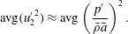 $$\begin{eqnarray}\text{avg}({u_{2}^{\prime }}^{2})\approx \text{avg}\left(\frac{p^{\prime }}{\bar{\unicode[STIX]{x1D70C}}\bar{a}}\right)^{2}.\end{eqnarray}$$
This represents a state of equipartition which will be verified later by DNS results.
2.3 Perturbation behaviour at different asymptotic limits
2.3.1 Spanwise modes (
$\unicode[STIX]{x1D6FD}=90$
)

First we examine spanwise perturbation modes:
 $\unicode[STIX]{x1D6FD}=\unicode[STIX]{x03C0}/2$
;
 $\unicode[STIX]{x1D705}_{1}=0$
and
 $\unicode[STIX]{x1D705}_{3}=1$
. For all such perturbations, equations (2.50) and (2.51) indicate a decoupling of the
 $p^{\prime }$
and
 $u_{2}^{\prime }$
fields at all Mach numbers as
 $\cos \unicode[STIX]{x1D6FD}=0$
. Referring to (2.39), it can be surmised that the
 $u_{1}^{\prime }$
component is also unaffected by pressure as
 $\unicode[STIX]{x1D705}_{1}=0$
. Clearly, both
 $u_{1}^{\prime }$
and
 $u_{2}^{\prime }$
fields are impervious to the pressure field. Thus, spanwise perturbation behaviour can be expected to be independent of Mach number. In the incompressible case, the pressure-free growth of spanwise modes is referred to as the lift-up mechanism by Ellingsen & Palm (Reference Ellingsen and Palm1975), Landahl (Reference Landahl1980) and Hanifi & Henningson (Reference Hanifi and Henningson1998). Our analysis indicates that the lift-up mechanism is preserved intact at all incompressible and compressible Mach numbers.
2.3.2 Streamwise modes (
$\unicode[STIX]{x1D6FD}=0$
)

Next we turn our attention to streamwise modes:
 $\unicode[STIX]{x1D6FD}=0;\unicode[STIX]{x1D705}_{1}=1$
and
 $\unicode[STIX]{x1D705}_{3}=0$
. It is well established in the literature that as
 $M_{g}\rightarrow 0$
, equations (2.50)–(2.51) for streamwise perturbations (
 $\unicode[STIX]{x1D6FD}=0$
) lead to TS waves. At larger
 $M_{g}$
,
 $p^{\prime }$
assumes a wave-like character as dictated by its evolution equation. The resulting
 $u_{2}^{\prime }$
field is not solenoidal, leading to dilatational velocity fluctuations. The pressure-induced oscillations in
 $u_{2}^{\prime }$
can be expected to have a profound effect on instability evolution as neither kinetic energy production or vorticity production can be sustained. One of the objectives of this work is to examine how the perturbation evolution is modified.
2.3.3 Uniform shear flow
To infer the behaviour of perturbation modes of intermediate degrees of obliqueness, further simplifications of the governing equations are needed. We examine the interactions in uniform shear flow as it is amenable to more rigorous mathematical treatment. In other words, we propose that a reasonable characterization of obliqueness effect on pressure–velocity interactions can be obtained by simplifying the shear as locally constant. This simplification is similar to the WKB-based local stability analysis of Lifschitz & Hameiri (Reference Lifschitz and Hameiri1991). Baines, Majumdar & Mitsudera (Reference Baines, Majumdar and Mitsudera1996) also invoke such a simplification in analysing the TS waves in incompressible flows. It must be reiterated that the objective here is to develop a qualitative understanding of the pressure–velocity interactions unencumbered by the complexities introduced by any spatial variation of shear. The utility and validity of the simplification can be assessed later by comparing the analytical outcome against DNS results that fully account for spatial variations of shear, viscous effects, etc.
A detailed analysis of these equations in homogeneous flows is performed by Kumar et al. (Reference Kumar, Bertsch and Girimaji2014) and their conclusions on the effect of perturbation obliqueness on pressure–velocity interactions are now summarized. For an arbitrary oblique wave vector, we define the effective shear, the effective shear,
 $S_{e}$
, as:
 $$\begin{eqnarray}S_{e}=S\cos \unicode[STIX]{x1D6FD}.\end{eqnarray}$$
Next, we define an effective gradient Mach number for a mode of arbitrary obliqueness:
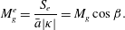 $$\begin{eqnarray}M_{g}^{e}=\frac{S_{e}}{\bar{a}|\unicode[STIX]{x1D705}|}=M_{g}\cos \unicode[STIX]{x1D6FD}.\end{eqnarray}$$
The effective Mach number
 $M_{g}^{e}$
of a perturbation mode, rather than the planar Mach number
 $M_{g}$
, is the appropriate dimensionless parameter to characterize the pressure–velocity interactions.
At high effective Mach number
 $(M_{g}^{e}>1)$
, there exist two distinct regimes of pressure–inertia interaction in the momentum equation. At early times
 $S_{e}t<\sqrt{M_{g}^{e}}$
, pressure perturbation evolves too slowly to affect velocity perturbation evolution. This is called the pressure-released (PR) stage, Kumar et al. (Reference Kumar, Bertsch and Girimaji2014). For a given planar Mach number and obliqueness angle, the duration of the pressure-released stage,
 $t_{PR}$
is given by
 $$\begin{eqnarray}0<t_{PR}<\sqrt{M_{g}/\cos \unicode[STIX]{x1D6FD}}.\end{eqnarray}$$
During this period, perturbations at all oblique angles can be expected to exhibit lift-up mechanism behaviour. This will be later verified using DNS results. Beyond this time, pressure evolves rapidly enough to counter the inertial effects. At this stage,
 $p^{\prime }$
and
 $u_{2}^{\prime }$
evolves as a simple harmonic oscillator.
2.4 Summary of analysis
We can now summarize the various inferences from the linear analysis.
-
(i) Irrespective of the gradient Mach number, spanwise (
$\unicode[STIX]{x1D6FD}=90^{\circ }$
or
$\unicode[STIX]{x1D705}_{1}=0$
) modes are unaffected by pressure. Thus, the lift-up mechanism is preserved intact at all Mach numbers. -
(ii) For a given planar Mach number (
$M_{0}$
), streamwise (
$\unicode[STIX]{x1D6FD}=0^{\circ }$
or
$\unicode[STIX]{x1D705}_{3}=0$
) modes experience highest effective Mach number. Thus, streamwise modes that lead to TS waves in incompressible flows can be expected to experience most significant compressibility effects in high-speed flows. -
(iii) Modes of increasing level of obliqueness can be expected to experience progressively decreasing compressibility effects. Indeed, there exists a critical obliqueness angle,
$\unicode[STIX]{x1D6FD}_{c}$
which experiences unit effective Mach number. (2.60)
$$\begin{eqnarray}M_{g}^{e}(\unicode[STIX]{x1D6FD}_{c})=1;\quad \unicode[STIX]{x1D6FD}_{c}=\cos ^{-1}\left(\frac{1}{M_{0}}\right).\end{eqnarray}$$
$\unicode[STIX]{x1D6FD}_{c}$
demarcates the perturbation–orientation space into two regions. All modes with
$\unicode[STIX]{x1D6FD}<\unicode[STIX]{x1D6FD}_{c}$
are classified as supersonic as their effective Mach number is greater than unity. Modes with
$\unicode[STIX]{x1D6FD}>\unicode[STIX]{x1D6FD}_{c}$
are identified as subsonic modes. Oblique modes with
$\unicode[STIX]{x1D6FD}>\unicode[STIX]{x1D6FD}_{c}$
are likely to be less affected by compressibility and retain their subsonic character. Whereas, velocity perturbations of modes with
$\unicode[STIX]{x1D6FD}<\unicode[STIX]{x1D6FD}_{c}$
are likely to be significantly affected by compressibility effects.
-
(iv) All perturbations experience an initial PR state. During this period, the behaviour is similar to that of lift-up modes. The duration of the PR state increases with Mach number and obliqueness angle. Compressibility effects manifest beyond this period.
-
(v) At high Mach numbers,
$p^{\prime }$
and
$u_{2}^{\prime }$
are coupled as a harmonic oscillator and each variable will exhibit oscillatory behaviour. When averaged over long periods of time, the potential energy contained in
$p^{\prime }$
and dilatation turbulent kinetic energy in
$u_{2}^{\prime }$
should be nearly equal – in a state of equipartition. -
(vi) All of the above behaviour can be expected to manifest independent of the mode profile shape in the stream-normal direction.





We will next examine these analytical inferences by performing DNS of small perturbation evolution in parabolic Poiseuille flow. The DNS study incorporates both nonlinear and viscous effects not considered in the linear analysis.
3 Numerical scheme for DNS
Numerical simulations are performed using a gas kinetic method (GKM) solver. The GKM solves the Boltzmann equations for the single particle probability density function
 $f$
using a linear collision operator (Xu Reference Xu2001). The numerical discretization is applied to the fundamental quantity, the distribution function
 $f$
, rather than the continuum variables. The constitutive relationships are computed as moments of the distribution function leading to consistent representations between various discretized conservation equations and precluding additional viscous/conductive flux discretization (May, Srinivasan & Jameson Reference May, Srinivasan and Jameson2007). The main attribute of GKM is that it provides a good numerical platform for considering non-equilibrium and non-continuum effects. The current continuum-limit GKM code has been well tested in decaying and homogeneous turbulence flows (Kerimo & Girimaji Reference Kerimo and Girimaji2007; Kumar, Girimaji & Kerimo Reference Kumar, Girimaji and Kerimo2013; Kumar et al.
Reference Kumar, Bertsch and Girimaji2014). In these studies, the GKM compressible homogeneous shear turbulence DNS results are compared against RDT and previous simulations in the literature resulting in excellent agreement. In recent work (Xie & Girimaji Reference Xie and Girimaji2014), the solver has been extended to wall-bounded shear flow. The background flow is sustained using a body force. A detailed verification and convergence study of the solver is presented in the Appendix.
Initial base flow conditions.

Simulation parameters. In the current study, the computational domain is a rectangular box of dimension
 $L_{x_{1}}\times L_{x_{2}}\times L_{x_{3}}:$
 $4L\times L\times 0.8L$
. Grid cells are uniformly distributed along
 $x_{1}$
and
 $x_{3}$
directions. Along the wall-normal direction,
 $x_{2}$
, the grids are distributed in geometric progression. The geometric progression coefficient is
 $1.0125$
. The grid is symmetric about the channel centreline. For all cases, the cell resolution is
 $N_{x_{1}}\times N_{x_{2}}\times N_{x_{3}}=160\times 200\times 32$
. The details of the simulation cases undertaken in the current study are given in table 1, where
 $U_{0}$
is the initial base flow velocity at the centreline,
 $\unicode[STIX]{x1D70C}_{0}$
is the initial base flow density and
 $T$
is the initial base flow temperature. The Mach number (
 $M_{0}=U_{0}/\bar{a}$
) is based on the centreline base velocity. The Reynolds (
 $Re=\unicode[STIX]{x1D70C}U_{0}L/\unicode[STIX]{x1D707}$
) number is based on unit length scale. The various simulation parameters are chosen to be of the same order as that of Sivasubramanian & Fasel (Reference Sivasubramanian and Fasel2014). Further, these parameters fall into the range of flows that are investigated in the experimental facility at Texas A&M University (Tichenor, Humble & Bowersox Reference Tichenor, Humble and Bowersox2013).
Boundary conditions. Periodic boundary conditions are applied in the
 $x_{1}$
and
 $x_{3}$
directions. In the
 $x_{2}$
direction, no-slip and no-penetration wall conditions are applied. Adiabatic and isothermal conditions are examined, and both boundary conditions yield similar perturbation evolution while the base temperature and density profiles show minor variations. Simulations performed using the isothermal wall condition are presented here similarly as the work of Xie & Girimaji (Reference Xie and Girimaji2014).
Initial conditions. A time-invariant parabolic base flow is first generated using a body force (Xie & Girimaji Reference Xie and Girimaji2014). The body force is chosen such that pressure, density and temperature fields are initially spatially uniform (see table 1). A perturbation velocity field is superposed on the base flow and allowed to evolve. The body force is maintained to sustain the parabolic base flow. It is found that, even at the end of the simulation, the mean density and temperature fields are close to spatially uniform at all times under the given conditions. Thus, we isolate the effects of high Mach number effects from those due to variations in the background thermodynamic state.
The magnitude of initial perturbation is set to
 $0.5\,\%$
of the value of the centreline base velocity. The linear analysis of the previous section is valid for arbitrary perturbation profiles in the wall-normal
 $x_{2}$
-direction. As mentioned before, the goal of the study is to examine the fundamental features of pressure–velocity interactions for any arbitrary initial perturbation. Towards that end, we focus on three different initial perturbation profiles.
-
(i) The incompressible Orr–Sommerfeld (OS) perturbation mode (Davey Reference Davey1973) that leads to flow instability in low-speed flows. This is similar to the initial condition used by Liang, Premasuthan & Jameson (Reference Liang, Premasuthan and Jameson2009) to study the transition to turbulence in high-speed channel flow. In that study, it is demonstrated that the resulting high Mach number channel flow captures the essential features of near-wall behaviour. Further, the use of this initial condition permits direct comparison between well-established incompressible flow behaviour and its compressible counterpart. Such comparison serves to isolate the effect of compressibility without the complicating influence of other features.
-
(ii) Next we examine an arbitrary perturbation profile that satisfies the boundary conditions and divergence-free constraint initially:
(3.1)
$$\begin{eqnarray}\displaystyle & \displaystyle u_{1}^{\prime }\approx U_{0}\sin \left(2\unicode[STIX]{x03C0}\frac{x_{1}}{L_{x_{1}}}\right)\sin \left(2\unicode[STIX]{x03C0}\frac{x_{2}}{L_{x_{2}}}\right), & \displaystyle\end{eqnarray}$$
(3.2)
$$\begin{eqnarray}\displaystyle & \displaystyle u_{2}^{\prime }\approx U_{0}\left(\frac{L_{x_{2}}}{L_{x_{1}}}\right)\sin \left(2\unicode[STIX]{x03C0}\frac{x_{1}}{L_{x_{1}}}\right)\cos \left(2\unicode[STIX]{x03C0}\frac{x_{2}}{L_{x_{2}}}+1\right), & \displaystyle\end{eqnarray}$$
(3.3)
$$\begin{eqnarray}\displaystyle & \displaystyle u_{3}^{\prime }=0. & \displaystyle\end{eqnarray}$$
-
(iii) The third perturbation is taken to be a simple linear superposition of the arbitrary and OS profiles, called the combined mode.



If all three perturbation profiles yield similar pressure–velocity interactions which are also consistent with linear theory, then one can cautiously infer that to be the general behaviour.
4 Simulation results
The objective of the study is to contrast small perturbation evolution in low and high Mach number wall-bounded flows and explain the difference in the underlying flow mechanisms. Our interest here is confined to linear stability considerations. Thus only evolution of single initial perturbation mode is considered. Four investigations are undertaken:
-
(i) evolution of OS mode profile at low Mach numbers and different obliqueness angles;
-
(ii) evolution of OS mode profile at high Mach numbers and different obliqueness angles;
-
(iii) evolution of arbitrary mode profiles at high Mach number and different obliqueness angles;
-
(iv) effect of inhomogeneity on vorticity perturbation and the balance between linear and quadratic shear effects.
4.1 OS mode evolutions at low Mach numbers
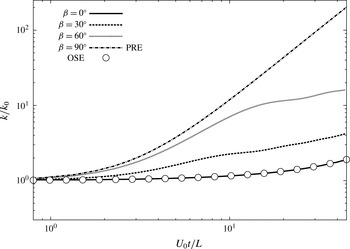
Incompressible evolution of perturbations at different obliqueness angles with initial OS mode profile is first presented. This will serve as the baseline case for examining the compressibility effects. The volume-averaged turbulent kinetic energy evolution for various
 $\unicode[STIX]{x1D6FD}$
values at the incompressible limit (
 $M_{0}=0.08$
) is given in figure 2. The incompressible analytical OS solutions for
 $\unicode[STIX]{x1D6FD}=0^{\circ }$
is also plotted in figure 2. Through the rest of the paper, the behaviour
 $\unicode[STIX]{x1D6FD}=0^{\circ }$
mode is referred to as the solution to the Orr–Sommerfeld equation (OSE). Excellent agreement between linear theory and DNS is evident for the TS mode.
Kinetic energy evolution of oblique modes at
 $M_{0}=0.08$
; OSE is the solution to the Orr–Sommerfeld equation for
 $\unicode[STIX]{x1D6FD}=0^{\circ }$
.
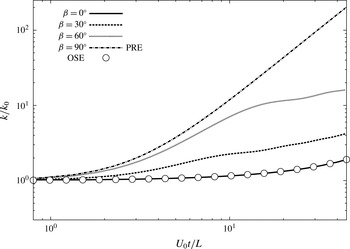
For
 $\unicode[STIX]{x1D6FD}=90^{\circ }$
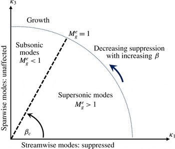
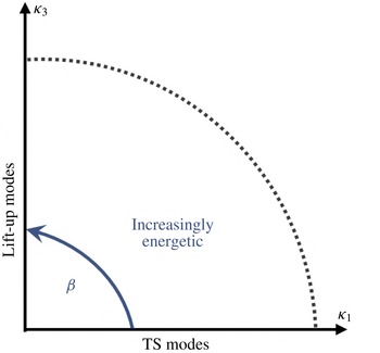
, the perturbation evolution exhibits more rapid growth. This is the lift-up behaviour discussed earlier in this paper (Landahl Reference Landahl1980). Perturbation modes with intermediate angles also exhibit increasing growth rate at this low-speed limit. The growth rate of intermediate obliqueness modes fall between the limits set by TS and lift-up modes. Overall, perturbation modes of all obliqueness angles exhibit growth. The dependence of perturbation evolution on obliqueness angle in low-speed Poiseuille flow is summarized in the schematic in figure 3.
Dependence of growth rate on perturbation obliqueness in incompressible Poiseuille flow.
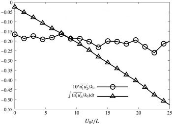
Shear Reynolds stress and its time integration evolution at
 $M_{0}=0.08$
: Reynolds stress is scaled by 10.
Reynolds shear stress
 $\overline{u_{1}^{\prime }u_{2}^{\prime }}$
plays an important role in the production of kinetic energy. Therefore, the evolution of shear Reynolds stress is examined for
 $\unicode[STIX]{x1D6FD}=0^{\circ }$
case at
 $x_{2}/L=0.1$
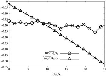
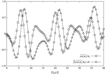
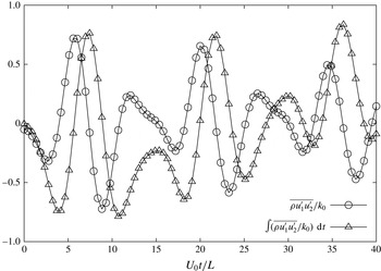
-plane. The Reynolds stress is obtained by plane averaging along the streamwise and spanwise directions. The Reynolds shear stress and its time-integral evolution are shown in figure 4. As previously stated, the normalized shear Reynolds stress is always negative and its time integral shows monotonic growth in magnitude with time. The time integral of
 $\overline{u_{1}^{\prime }u_{2}^{\prime }}$
corresponds to the total production of perturbation kinetic energy up to that point in time. This result will later be contrasted against the time integral of Reynolds shear stress in compressible flows.
4.2 OS mode evolution at high Mach numbers
Now we turn our attention to the evolution of OS profile modes in compressible flows. The OS perturbation is introduced at different obliqueness angles and the evolution is examined. The results are presented according to obliqueness angles.
4.2.1 Lift-up mode (
$\unicode[STIX]{x1D6FD}=90^{\circ }$
)

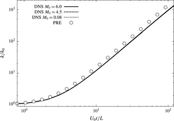
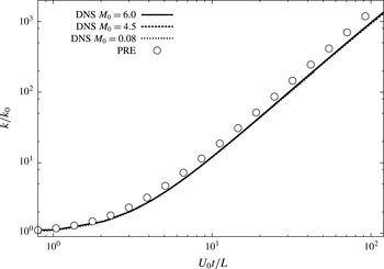
Linear analysis clearly indicates that the evolution of spanwise modes should be nearly identical at all reference Mach numbers. The DNS results of volume-averaged turbulent kinetic energy evolution at
 $M_{0}=0.08$
,
 $4.5$
and
 $6$
are shown in figure 5. The spanwise mode lift-up behaviour is indeed independent of Mach number. Furthermore, these results are in close agreement with the analytical solution of the pressure-released equation (PRE). The results clearly confirm that lift-up mechanism is intact at all Mach numbers.
Kinetic energy evolution of spanwise perturbation.
4.2.2 Streamwise mode (
$\unicode[STIX]{x1D6FD}=0^{\circ }$
)

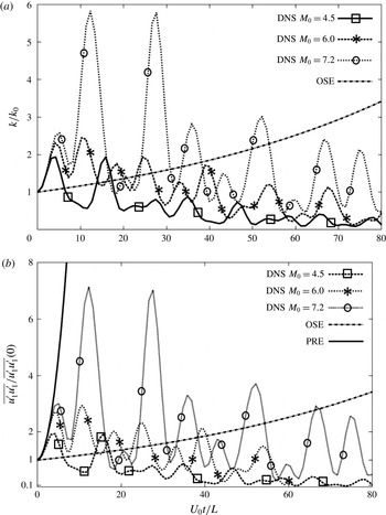
We present the DNS results for volume-averaged turbulent kinetic energy as well as volume-averaged
 $u_{1}^{\prime 2}$
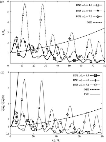
in figure 6. The DNS results from computations at different Mach numbers are compared against OSE and PRE analytical solutions. Initially, the growth of all three Mach number cases are identical and follow the PRE solution, confirming the findings of the linear analysis. As explained earlier, the pressure perturbation effects are initially insignificant leading to a lift-up type of behaviour. The pressure fluctuations build up with time as the perturbations enter the second phase of their evolution. Then, the perturbation growth departs from the PRE limit as soon as the pressure effects become significant. The figure also shows that the higher the Mach number, the later is the departure from PRE behaviour, once again in line with the analysis presented in § 2. The subsequent evolution demonstrates oscillatory behaviour as suggested by the linear analysis due to the emergence of a dilatational velocity fluctuation. Eventually, the kinetic energy reduces to levels much lower than the TS perturbation energy in incompressible flow. It is evident that the instability is suppressed due to the action of the oscillatory dilatational field.
Evolution of streamwise perturbation in high Mach number flows: (a) turbulent kinetic energy and (b)
 $\overline{u_{1}^{\prime }u_{1}^{\prime }}$
.
Now we seek the physical explanation underlying the stabilization of the streamwise perturbation mode. The linear analysis of § 2 indicates that the
 $u_{2}^{\prime }$
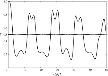
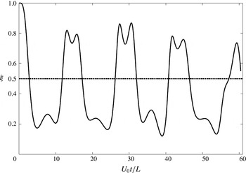
component is coupled to pressure as in a harmonic oscillator leading to equipartition of energy between them. To verify this inference, in figure 7 we plot volume-averaged
 ${u_{2}^{\prime }}^{2}$
and
 $p^{\prime 2}$
for the case of
 $M_{0}=6$
. As anticipated, the potential energy and dilatational kinetic energy oscillate about the equipartition level. Linear analysis further indicates that this behaviour should lead to oscillations in the all-important Reynolds shear stress
 $\overline{\unicode[STIX]{x1D70C}u_{1}^{\prime }u_{2}^{\prime }}$
.
Energy equipartition between wall-normal velocity and pressure perturbation at
 $M_{0}=6$
.
 $\unicode[STIX]{x1D709}=(\overline{u_{2}^{\prime }u_{2}^{\prime }})/(u_{2}^{\prime }u_{2}^{\prime }+\overline{p^{\prime }p^{\prime }}/(\unicode[STIX]{x1D6FE}\unicode[STIX]{x1D70C}\bar{p}))$
.
The Reynolds stress component
 $\overline{\unicode[STIX]{x1D70C}u_{1}^{\prime }u_{2}^{\prime }}$
is plotted in figure 8 as a function of time for
 $M_{0}=6$
case. The time integral of the stress is also shown as this corresponds to the total production up to that instant in time. The contrast between the incompressible (figure 4) and compressible (figure 8) shear stress evolution is immediately evident. Unlike its low Mach number counterpart, the compressible Reynolds stress shows large oscillations covering negative and positive values. As a result, the integral stays close to zero despite large initial excursions toward negative values. Thus, the kinetic energy does not exhibit sustained growth leading to stabilization. In summary, the streamwise perturbation mode is suppressed in high-speed flows due to the action of pressure which creates oscillations in
 $\overline{\unicode[STIX]{x1D70C}u_{1}^{\prime }u_{2}^{\prime }}$
spanning both positive and negative values.
Shear Reynolds stress and its time integration evolution at
 $M_{0}=6$
.
4.2.3 Oblique modes (
$0^{\circ }<\unicode[STIX]{x1D6FD}<90^{\circ }$
)

For oblique modes with angles between
 $0^{\circ }$
and
 $90^{\circ }$
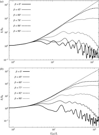
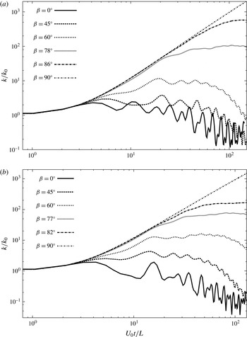
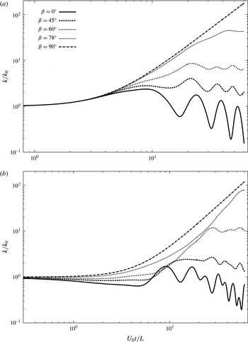
, the individual perturbations are investigated by examining the volume-averaged turbulent kinetic energy evolution shown in figure 9 for two Mach numbers. At early times modes, all oblique modes follow the PRE evolution for some duration. Consistent with linear analysis, the more oblique the mode, the longer is the duration of the PR (or lift-up) behaviour. At later times, the streamwise mode evolution exhibits the most oscillations due to the action of pressure. The oscillations become weaker with increasing
 $\unicode[STIX]{x1D6FD}$
. Moreover, with increasing
 $\unicode[STIX]{x1D6FD}$
, the perturbations become more energetic and approach the pressure-released limit at
 $\unicode[STIX]{x1D6FD}=90^{\circ }$
. This is completely consistent with linear theory wherein it is shown that the effective Mach number decreases with
 $\unicode[STIX]{x1D6FD}$
, and the effect of compressibility diminishes correspondingly.
Kinetic energy evolution of oblique modes: (a)
 $M_{0}=6$
and (b)
 $M_{0}=4.5$
.
Next we investigate the significance of the critical angle (
 $\unicode[STIX]{x1D6FD}_{c}$
) identified in the linear analyses. For
 $M_{0}=4.5$
and
 $6$
cases, the
 $\unicode[STIX]{x1D6FD}_{c}$
values are approximately
 $77^{\circ }$
and
 $80^{\circ }$
respectively. Referring to figure 9, the following observations can be made.
-
(i) For
$\unicode[STIX]{x1D6FD}<\unicode[STIX]{x1D6FD}_{c}$
, the computational results indicate asymptotic decline of kinetic energy. Evidently, this is due to the oscillatory coupling between
$u_{2}^{\prime }$
and
$p^{\prime }$
. -
(ii) The kinetic energy of
$\unicode[STIX]{x1D6FD}\geqslant \unicode[STIX]{x1D6FD}_{c}$
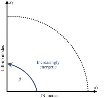
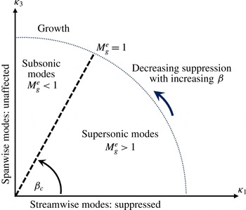
modes do not display oscillations. These modes are not discernibly suppressed by compressibility effects and their evolution is nearly similar to their incompressible counterparts. Most importantly, the growth continues over the duration of simulation. These findings are summarized in the schematic in figure 10.


Dependence of kinetic energy growth rate on obliqueness in compressible Poiseuille flow.
All discussions thus far have focused on initial perturbation profile taken from the Orr–Sommerfeld analysis of an incompressible Poiseuille flow. The intent was to examine how TS waves (streamwise) and lift-up (spanwise) modes are affected at high speeds. Now we examine other perturbation profiles to ensure the validity of the inferences summarized above.
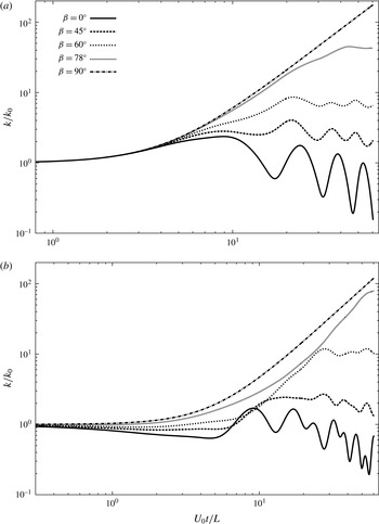
Kinetic energy evolution of arbitrary and combined perturbation modes, defined in § 3, is examined in figure 11 at
 $M_{0}=6$
. It is evident that
 $\unicode[STIX]{x1D6FD}=0^{\circ }$
perturbation is still suppressed. The large oscillations indicate the effect of dilatational velocity fluctuations. The
 $\unicode[STIX]{x1D6FD}=90^{\circ }$
modes again grow monotonically and do not exhibit any Mach number effect. At intermediate angles, the growth rate gradually increase as indicated by linear analysis and summarized in the schematic in figure 10.
It is important to completely reconcile the PR stage with the lift-up mechanism in the literature. The connection can be surmised from the following observations.
-
(i) Spanwise perturbations of all supersonic Mach numbers experience a prolonged PR state and the kinetic energy exhibits algebraic growth (see figure 5). This is the well-established lift-up effect.
-
(ii) At high Mach numbers, modes of all angles experience a short duration of PR state. As established in the linear analysis, the duration of PR state increases with Mach number
$M_{0}$
and obliqueness angle
$\unicode[STIX]{x1D6FD}$
. From figure 6, it is evident that even streamwise modes experience a lift-up type of growth at the early PR stage. Figures 9 and 11 demonstrate the effect of obliqueness and initial mode shape. From figure 9, it is evident that oblique modes exhibit lift-up behaviour for a longer duration as suggested by linear analysis. Figure 11 clearly demonstrates that the obliqueness effect is independent of the initial perturbation profile. Thus lift-up behaviour is seen at early times independent of Mach number (so long as it is high) and obliqueness. -
(iii) The deviation from lift-up behaviour occurs due to the action of pressure. Pressure effects come into play faster at (i) lower Mach numbers; and (ii) lower obliqueness angles.
-
(iv) Equipartition (over a cycle of oscillation) is observed immediately following the PR stage.


Evolution of kinetic energy for other initial modes at
 $M_{0}=6$
: (a) arbitrary mode and (b) combined mode.
4.3 Effect of inhomogeneity on vorticity
The results presented thus far are consistent with the linear analysis of the pressure equation in which the spatial variation of shear is neglected. To establish the effect of shear variation we examine the vorticity budget for
 $\unicode[STIX]{x1D6FD}=0$
OS mode. This will provide further insight into how the incompressible perturbation vorticity is suppressed in compressible flows.
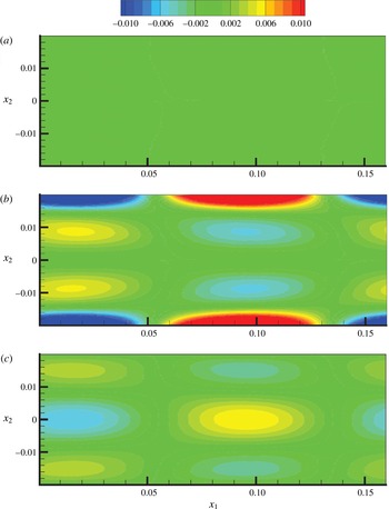
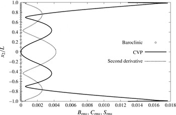
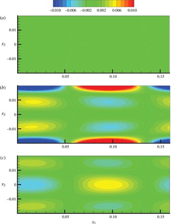
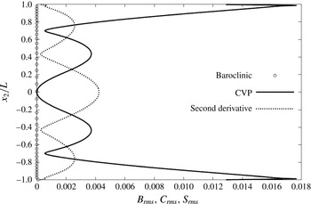
We focus on the spanwise vorticity equation given in (2.26). There are three important terms on the right-hand side of the equation as the viscous effect is not significant in the duration considered. As mentioned before, the baroclinic term and compressible vorticity production correspond to the compressibility effects. The second derivative term is pertinent in both the incompressible and compressible flow regimes. In high Mach number Poiseuille flow, the three mechanisms are examined using DNS data in figure 12. At a given time instant, a contour plot of each significant vorticity term in the
 $x{-}y$
plane is shown. The planar root-mean-square of each term at that same instance is shown in figure 13. It is immediately evident that there are three distinct regions as suggested by linear analysis in § 2.2. Adjacent to each wall, there is a region in which CVP is completely dominant. It is in this region that TS waves typically develop in incompressible flows. Here, the compressible effects preclude the formation of such waves. In the central region, occupying 75 % of the channel height, the CVP and second derivative effects are nearly equal and out of phase. This region does not contribute much to the flow dynamics at any speed. The baroclinic term is negligible at all locations. This is to be expected as background density variation is not considered in this study.
Spanwise vorticity budget term at
 $M_{0}=6$
: (a) baroclinic term, (b) compressible vortex production term and (c) second derivative term.
Root mean square of vorticity budget: baroclinic, CVP and the second derivative. All terms are defined in (2.26).
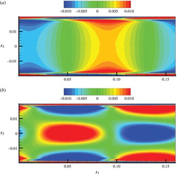
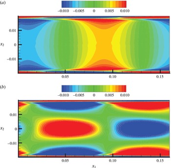
To examine the consequence of the CVP effect, the spanwise vorticity contours for both low- and high-speed Poiseuille flow are given in figure 14. The vorticity is normalized by the base flow centreline velocity
 $U_{0}$
and length scale
 $L$
. In the incompressible case, a single vortex structure spans the entire channel height. On the other hand, the high Mach number case exhibits three distinct vortical structures across the channel height corresponding to the three regions of CVP identified in figure 12.
Spanwise vorticity contours in low-speed and high-speed flows: (a)
 $M_{0}=0.12$
and (b)
 $M_{0}=6$
.
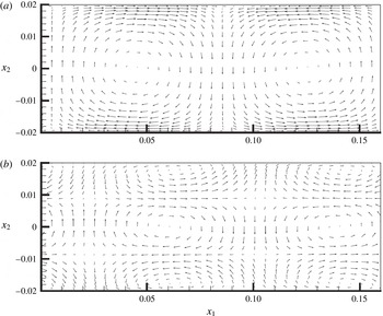
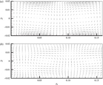
The corresponding perturbation velocity vectors are plotted in figure 15 for
 $M_{0}=0.08$
and
 $6$
. The difference in the structure at the two speeds is clearly evident. The circulation in the incompressible case covers the entire channel height resulting in efficient momentum transfer from the centre of the flow to the walls. The flow in the high-speed case is separated into three distinct regions across the channel height as previously observed. Each near-wall region exhibits pulsating motion within its domain. The circulation in the centre does not penetrate all the way to the wall. Therefore, there is reduced momentum mixing between the centre and the walls.
Typical flow structures of both low-speed and high-speed flow: (a)
 $M_{0}=0.12$
and (b)
 $M_{0}=6$
.
5 Conclusion
The objective of this work is to examine the effect of dilatational fluctuations on small perturbation growth in wall-bounded high-speed shear flows. The character of pressure–velocity interactions and the consequent effect on perturbation evolution is characterized at different flow speeds. Linear analysis of the pertinent initial value problem highlights the importance of perturbation obliqueness and leads to crucial inferences. The inferences are then examined using DNS of small perturbation evolution at different Mach numbers. The main conclusions are as follows.
-
(i) Spanwise perturbation mode evolution is impervious to Mach number in Poiseuille flows. Thus the lift-up mechanism is preserved intact in high-speed wall-bounded flows.
-
(ii) Streamwise disturbances that lead to TS waves at low speeds are profoundly affected by compressibility. The oscillatory nature of
$u_{2}^{\prime }$
evolution prevents sustained growth of turbulent kinetic energy. These oscillations also prevent the formation of strong vortex structures in the near-wall region. -
(iii) Perturbations of intermediate levels of obliqueness experience varying degrees of suppression. Indeed, perturbations aligned close to the spanwise direction experience subsonic Mach numbers and hence very limited suppression.
-
(iv) The potential energy incumbent in the pressure fluctuations and dilatational kinetic energy in the wall-normal velocity fluctuations are in a state of equipartition.
-
(v) The high-speed Poiseuille flow domain is partitioned into three different regions: two compressibility-dominated near-wall regions and a central region. The dilatational fluctuations in the near-wall regions isolate the wall from the central region leading to diminished momentum exchange.

Development of closure models for predictive computations of transition and turbulence in high-speed flows requires an intimate knowledge of pressure action at different flow speeds. This work represents a first step in that direction. Pressure–strain correlation closure models based on these findings have already been developed and were found to be successful in the computation of high-speed boundary layers and mixing layers (Gomez & Girimaji Reference Gomez and Girimaji2013, Reference Gomez and Girimaji2014). While more work is needed to fully understand compressibility effects on transition to turbulence in high-speed wall-bounded flow, this work explicates some of the important pressure–velocity interactions and the consequent influence on perturbation evolution.
Acknowledgements
This work was supported by the National Center for Hypersonic Laminar-Turbulent Transition Research at Texas A&M University. The authors would like to thank Dr W. Saric for his support and guidance.
Appendix. Numerical scheme validation and verification
At the low Mach number limit, the GKM results show excellent agreement with the OS solution in figure 5 of Xie & Girimaji (Reference Xie and Girimaji2014). Calculations with three initial perturbation levels are performed and the evolution of normalized perturbation magnitude from each case is compared against the analytical solution of the OSE. The numerical and analytical results are in excellent agreement, demonstrating the validity of the code at low speeds. Next we verify the code at the limit of very high Mach number. At the limit of high Mach number, the GKM results are compared against analytical solutions obtained from the PRE. For a detailed description of the pressure-released limit and PRE in wall-bounded flows, the reader is referred to Ellingsen & Palm (Reference Ellingsen and Palm1975), Hanifi & Henningson (Reference Hanifi and Henningson1998) and Xie & Girimaji (Reference Xie and Girimaji2014). It is shown that the GKM results for the three different Mach numbers agree well with the PRE analytical solution at the early stage when pressure effects are negligible (figure 2 of Xie & Girimaji (Reference Xie and Girimaji2014)). This is in complete agreement with the linear analysis results presented earlier in the paper. Moreover, the departure from the PRE solution scales according to theoretical estimate as shown by Xie & Girimaji (Reference Xie and Girimaji2014).
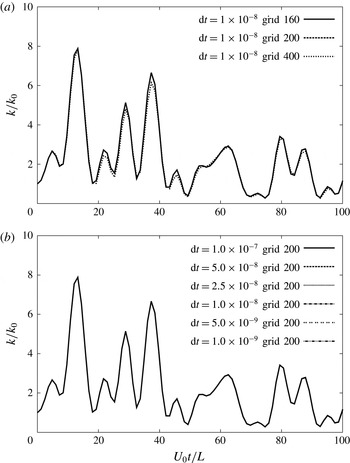
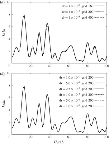
A convergence study for grid resolution and time step is performed and the results are shown in figure 16. Many different grid sizes and time steps are examined. The results are nearly grid independent at the resolutions and time steps used in the study.
Convergence study at
 $M_{0}=8$
: (a) grid resolution study and (b) time step study.
 $k_{0}$
is the initial perturbation kinetic energy. The number in the notation indicates the grid points in the wall-normal direction.