2.1 Flow expansion

The total flow is modelled by the full compressible Navier–Stokes equations. The acoustic wave streamwise velocity amplitude $u_{a,\infty }^{\ast }$ is considered to be small with respect to the free-stream velocity $\bar{U}_{\infty }$ , whereas the maximum amplitude of the wall perturbation $a_{w}^{\ast }$ is small compared to the reference scale $l_{w}^{\ast }$ . The definitions of $a_{w}^{\ast }$ and $l_{w}^{\ast }$ depend on the wall perturbation mechanism: (i) for surface roughness, $a_{w}^{\ast }=h^{\ast }$ is the roughness height and $l_{w}^{\ast }=L$ is the flat plate chord; (ii) for a suction slot, $a_{w}^{\ast }=v_{s}^{\ast }$ is the wall-normal suction velocity and $l_{w}^{\ast }=\bar{U}_{\infty }$ ; (iii) for a heating strip, $a_{w}^{\ast }=\unicode[STIX]{x1D703}_{h}^{\ast }$ is the wall temperature differential and $l_{w}^{\ast }=\bar{T}_{\infty }$ is the far-field temperature. Thus we define two small parameters $\unicode[STIX]{x1D700}_{a}=u_{a,\infty }^{\ast }(\unicode[STIX]{x1D6E9}=0)/\bar{U}_{\infty }\ll 1$ and $\unicode[STIX]{x1D700}_{w}^{(j)}=a_{w}^{\ast }/l_{w}^{\ast }\ll 1$ , and introduce a double-parameter expansion of all flow quantities (Ruban Reference Ruban and Kozlov1985)

(2.1) $$\begin{eqnarray}\boldsymbol{q}(x,y,z,t)=\bar{\boldsymbol{q}}(x,y)+\unicode[STIX]{x1D700}_{w}^{(j)}\boldsymbol{q}_{w}(x,y)\text{e}^{\text{i}\unicode[STIX]{x1D6FD}z}+\unicode[STIX]{x1D700}_{a}\boldsymbol{q}_{a}(x,y)\text{e}^{-\text{i}\unicode[STIX]{x1D714}t}+\unicode[STIX]{x1D700}_{w}^{(j)}\unicode[STIX]{x1D700}_{a}\boldsymbol{q}_{b}(x,y)\text{e}^{\text{i}(-\unicode[STIX]{x1D714}t+\unicode[STIX]{x1D6FD}z)}+\cdots \,,\end{eqnarray}$$

where the index $j=1{-}3$ indicates the type of wall perturbation in the order that they were presented. A Cartesian frame of reference is positioned at the leading edge of the flat plate. The $x$ -axis is aligned with the streamwise direction. The fluid flow velocity component in this direction is denoted $u$ . In similar fashion, the $y$ -axis and $z$ -axis are aligned with the wall-normal and spanwise directions, and the velocity components are denoted $v$ and $w$ respectively. In addition to the velocity components, the vector $\boldsymbol{q}=[u,v,w,p,\unicode[STIX]{x1D70C},T]^{\text{T}}$ also contains the fluid flow pressure $p$ , density $\unicode[STIX]{x1D70C}$ and temperature $T$ . Time is denoted $t$ . The double-parameter expansion is truncated at order $\mathit{O}(\unicode[STIX]{x1D700}_{w}\unicode[STIX]{x1D700}_{a})$ , consisting of four terms: (i) the 2-D base flow denoted by an over-bar; (ii) a small steady component induced by a wall perturbation and denoted by the subscript $w$ ; a single harmonic of spanwise wavenumber $\unicode[STIX]{x1D6FD}$ is considered; (iii) the acoustically driven flow of frequency $\unicode[STIX]{x1D714}$ denoted by the subscript $a$ ; the 2-D free-stream acoustic wave is incident at an angle $\unicode[STIX]{x1D6E9}$ , where $\unicode[STIX]{x1D6E9}=0$ corresponds to a downstream travelling wave and $\unicode[STIX]{x1D6E9}=\unicode[STIX]{x03C0}$ corresponds to an upstream travelling wave; (iv) a small unsteady term arising from the bilinear interaction of the flow fields of order $\mathit{O}(\unicode[STIX]{x1D700}_{w})$ and $\mathit{O}(\unicode[STIX]{x1D700}_{a})$ ; this component is denoted with the subscript $b$ and models the instability emerging from the receptivity process. This flow expansion captures the different components of the total flow to first order.

Flow and material quantities are made non-dimensional as follows

(2.2) $$\begin{eqnarray}\left.\begin{array}{@{}c@{}}x={\displaystyle \frac{x^{\ast }}{L}},\quad y={\displaystyle \frac{y^{\ast }}{L}},\quad z={\displaystyle \frac{z^{\ast }}{L}},\quad t={\displaystyle \frac{t^{\ast }\bar{U}_{\infty }}{L}},\quad u={\displaystyle \frac{u^{\ast }}{\bar{U}_{\infty }}},\quad v={\displaystyle \frac{v^{\ast }}{\bar{U}_{\infty }}},\\ w={\displaystyle \frac{w^{\ast }}{\bar{U}_{\infty }}},\quad p={\displaystyle \frac{p^{\ast }}{\bar{\unicode[STIX]{x1D70C}}_{\infty }\bar{U}_{\infty }^{2}}},\quad \unicode[STIX]{x1D70C}={\displaystyle \frac{\unicode[STIX]{x1D70C}^{\ast }}{\bar{\unicode[STIX]{x1D70C}}_{\infty }}},\quad T={\displaystyle \frac{T^{\ast }}{\bar{T}_{\infty }}},\quad \unicode[STIX]{x1D707}={\displaystyle \frac{\unicode[STIX]{x1D707}^{\ast }}{\bar{\unicode[STIX]{x1D707}}_{\infty }}},\end{array}\right\}\end{eqnarray}$$

where we have introduced the dynamic viscosity $\unicode[STIX]{x1D707}$ . Dimensional quantities are represented with a $\ast$ superscript. The reference quantities are the chord of the flat plate $L$ and the far-field flow quantities denoted by the subscript  $\infty$ .

2.2 Unsteady compressible boundary layer

The governing equations are approximated by the unsteady boundary layer equations (see, for example, Duck Reference Duck1990) which suitably model the base flow and the acoustically driven flow to first order in a thin viscous wall layer (Ackerberg & Phillips Reference Ackerberg and Phillips1972). The underlying assumptions are high Reynolds number flow and long acoustic wavelength compared to boundary layer thickness. As opposed to the full Navier–Stokes equations, this system of equations is an attractive choice of physical model because of its parabolic character, allowing for an efficient streamwise marching numerical procedure.

2.2.1 Steady base flow

Let us denote $\bar{\boldsymbol{q}}=[\bar{U},\bar{V},\bar{W},\bar{P},\bar{\unicode[STIX]{x1D70C}},\bar{T}]^{\text{T}}$ the base flow quantities. We restrict our attention to 2-D flows, i.e. $\bar{W}=0$ . We introduce the generalised Howarth–Dorodnitsyn transformation (Moore Reference Moore1951; Stewartson Reference Stewartson1951)

(2.3) $$\begin{eqnarray}\unicode[STIX]{x1D702}=\left({\displaystyle \frac{\bar{U}_{e}^{\ast }}{\bar{\unicode[STIX]{x1D707}}_{e}^{\ast }\bar{\unicode[STIX]{x1D70C}}_{e}^{\ast }x^{\ast }}}\right)^{1/2}\int _{0}^{y^{\ast }}\bar{\unicode[STIX]{x1D70C}}^{\ast }\,\text{d}s,\end{eqnarray}$$

and the streamfunction

(2.4) $$\begin{eqnarray}\unicode[STIX]{x1D713}=(\bar{\unicode[STIX]{x1D70C}}_{e}^{\ast }\bar{\unicode[STIX]{x1D707}}_{e}^{\ast }\bar{U}_{e}^{\ast }x^{\ast })^{1/2}F(\unicode[STIX]{x1D702},x^{\ast }),\end{eqnarray}$$

with

(2.5a,b ) $$\begin{eqnarray}F_{\unicode[STIX]{x1D702}}={\displaystyle \frac{\bar{U}^{\ast }}{\bar{U}_{e}^{\ast }}},\quad S={\displaystyle \frac{\bar{T}^{\ast }}{\bar{T}_{e}^{\ast }}},\end{eqnarray}$$

where the subscript ‘ $e$ ’ denotes boundary layer edge quantities. For the purposes of this subsection we consider that all flow and material quantities are made non-dimensional using boundary layer edge quantities instead of the far-field quantities used in (2.2). The steady boundary layer equations are then simplified using (2.3)–(2.5), yielding

(2.6a ) $$\begin{eqnarray}\displaystyle & \displaystyle {\displaystyle \frac{\unicode[STIX]{x2202}(\unicode[STIX]{x1D719}F_{\unicode[STIX]{x1D702}\unicode[STIX]{x1D702}})}{\unicode[STIX]{x2202}\unicode[STIX]{x1D702}}}+cF_{\unicode[STIX]{x1D702}\unicode[STIX]{x1D702}}F+m_{1}(S-F_{\unicode[STIX]{x1D702}}^{2})=x(F_{\unicode[STIX]{x1D702}}F_{\unicode[STIX]{x1D702}x}-F_{\unicode[STIX]{x1D702}\unicode[STIX]{x1D702}}F_{x}), & \displaystyle\end{eqnarray}$$

(2.6b ) $$\begin{eqnarray}\displaystyle & \displaystyle {\displaystyle \frac{1}{\unicode[STIX]{x1D70E}}}{\displaystyle \frac{\unicode[STIX]{x2202}(\unicode[STIX]{x1D719}S_{\unicode[STIX]{x1D702}})}{\unicode[STIX]{x2202}\unicode[STIX]{x1D702}}}+cFS_{\unicode[STIX]{x1D702}}+\unicode[STIX]{x1D719}(\unicode[STIX]{x1D6FE}-1)M_{e}^{2}F_{\unicode[STIX]{x1D702}\unicode[STIX]{x1D702}}^{2}=x(F_{\unicode[STIX]{x1D702}}S_{x}-S_{\unicode[STIX]{x1D702}}F_{x}), & \displaystyle\end{eqnarray}$$

where

(2.7a-e ) $$\begin{eqnarray}\unicode[STIX]{x1D719}=\bar{\unicode[STIX]{x1D707}}\bar{\unicode[STIX]{x1D70C}},\quad m_{1}={\displaystyle \frac{x}{\bar{U}_{e}^{\ast }}}{\displaystyle \frac{\text{d}\bar{U}_{e}^{\ast }}{\text{d}x}},\quad m_{2}={\displaystyle \frac{x}{\bar{\unicode[STIX]{x1D707}}_{e}^{\ast }\bar{\unicode[STIX]{x1D70C}}_{e}^{\ast }}}{\displaystyle \frac{\text{d}(\bar{\unicode[STIX]{x1D707}}_{e}^{\ast }\bar{\unicode[STIX]{x1D70C}}_{e}^{\ast })}{\text{d}x}},\quad c={\displaystyle \frac{1}{2}}(1+m_{1}+m_{2}),\quad M_{e}^{2}={\displaystyle \frac{\bar{U}_{e}^{\ast ^{2}}}{\unicode[STIX]{x1D6FE}{\mathcal{R}}\bar{T}_{e}^{\ast }}}.\end{eqnarray}$$

The subscripts $\unicode[STIX]{x1D702}$ and $x$ indicate partial derivatives with respect to these variables. The Prandtl number, the specific heat ratio and the ideal gas constant are denoted $\unicode[STIX]{x1D70E}$ , $\unicode[STIX]{x1D6FE}$ and ${\mathcal{R}}$ , respectively. The usual no-slip and isothermal or adiabatic wall conditions are used.

2.2.2 Acoustic field

Let us consider a small amplitude acoustic wave travelling in the free stream with the unperturbed uniform steady flow,

(2.8) $$\begin{eqnarray}\boldsymbol{q}_{\infty }=\bar{\boldsymbol{q}}_{\infty }+\unicode[STIX]{x1D700}_{a}\boldsymbol{q}_{a,\infty }\unicode[STIX]{x1D712},\end{eqnarray}$$

where $\unicode[STIX]{x1D712}=\exp \{\text{i}\unicode[STIX]{x1D6FC}_{a}(-c_{a}t+x+\unicode[STIX]{x1D706}y)\}$ and $\bar{\boldsymbol{q}}_{\infty }=[1,0,0,\bar{p}_{\infty }/\bar{\unicode[STIX]{x1D70C}}_{\infty }\bar{U}_{\infty }^{2},1,1]^{\text{T}}$ . The streamwise wavenumber and phase speed are denoted $\unicode[STIX]{x1D6FC}_{a}$ and $c_{a}$ . The angle of incidence $\unicode[STIX]{x1D6E9}$ relates to $\unicode[STIX]{x1D706}$ in subsonic flows as

(2.9) $$\begin{eqnarray}\unicode[STIX]{x1D706}=\tan (\unicode[STIX]{x03C0}-\unicode[STIX]{x1D6E9}).\end{eqnarray}$$

The inviscid acoustic wave solution is known to be (Duck Reference Duck1990)

(2.10) $$\begin{eqnarray}c_{a}=1\pm {\displaystyle \frac{\sqrt{1+\unicode[STIX]{x1D706}^{2}}}{M_{\infty }}},\end{eqnarray}$$

(2.11a-d ) $$\begin{eqnarray}u_{a,\infty }={\displaystyle \frac{p_{a,\infty }}{c_{a}-1}},\quad v_{a,\infty }=\unicode[STIX]{x1D706}u_{a,\infty },\quad \unicode[STIX]{x1D703}_{a,\infty }=(\unicode[STIX]{x1D6FE}-1)M_{\infty }^{2}p_{a,\infty },\quad r_{a,\infty }=M_{\infty }^{2}p_{a,\infty },\end{eqnarray}$$

where $M_{\infty }$ is the far-field Mach number, and $\unicode[STIX]{x1D703}_{a}$ and $r_{a}$ are the temperature and density perturbations. The pressure perturbation $p_{a,\infty }$ is an independent variable determining the amplitude of the acoustic wave. For the purposes of this study we use $p_{a,\infty }=1/M_{\infty }$ , corresponding to the downstream travelling wave solution ( $u_{a,\infty }=1$ ). This maintains a constant sound pressure level for a coherent comparison of receptivity amplitudes at different angles of incidence.

The acoustic wave reflection is treated according to inviscid theory. This approach is valid provided the acoustic wavelength is long compared to the boundary layer thickness, which in turn is true if: (i) the free-stream Mach number is low, or (ii) the angle of incidence is shallow ( $\unicode[STIX]{x1D6E9}\rightarrow 0$ ). Under these assumptions, the boundary layer is not ‘seen’ by the acoustic wave, thus reflecting as if a solid wall is present (Mack Reference Mack1984). The wall-normal pressure gradient at the wall is zero according to the inviscid governing equations. The incident and reflected waves thus have the same amplitude and phase at the surface.

We now turn to the unsteady flow within the boundary layer. This motion is driven by the streamwise unsteady pressure gradient of the acoustic wave and can be modelled to first order by the LUBLE. Wall-normal unsteady pressure variations are neglected on the basis that the boundary layer thickness and the acoustic wavelength are not of comparable magnitude (Goldstein Reference Goldstein1985; Ruban Reference Ruban and Kozlov1985). We superimpose a perturbation on the base flow quantities

(2.12) $$\begin{eqnarray}\boldsymbol{q}=\bar{\boldsymbol{q}}+\unicode[STIX]{x1D700}_{a}\boldsymbol{q}_{a}\unicode[STIX]{x1D717},\end{eqnarray}$$

where $\unicode[STIX]{x1D717}=\exp \{\text{i}(-\unicode[STIX]{x1D714}t+\unicode[STIX]{x1D6FC}_{a}x)\}$ . It should be noted that formally we have assumed

(2.13) $$\begin{eqnarray}\boldsymbol{q}_{a}(x,y)=\hat{\boldsymbol{q}}_{a}(x,y)\text{e}^{\text{i}\unicode[STIX]{x1D6FC}_{a}x},\end{eqnarray}$$

but for the purposes of this section we have dropped the hat notation for simplicity. In a flat plate, the base flow has a similarity solution $(F_{\unicode[STIX]{x1D702}}(\unicode[STIX]{x1D702}),S(\unicode[STIX]{x1D702}))$ . Moreover, the far-field and boundary layer edge quantities coincide. With this in mind, the equations governing the acoustic layer are obtained by (i) substituting (2.12) in the unsteady boundary layer equations, (ii) subtracting the mean flow and (iii) performing a change of variable according to (2.3). We consider $\unicode[STIX]{x1D706}\neq 0$ , and thus the unsteady pressure gradient is $\text{d}p/\text{d}x=2\text{i}\unicode[STIX]{x1D700}_{a}\unicode[STIX]{x1D6FC}_{a}/M_{\infty }\unicode[STIX]{x1D717}$ , where the factor of 2 accounts for the reinforcement of the acoustic wave due to the inviscid nature of the reflection at the wall. One then obtains the linearised continuity, $x$ -momentum and energy equations, in this order

(2.14) $$\begin{eqnarray}\displaystyle & & \displaystyle \left(\text{i}\unicode[STIX]{x1D6FC}_{a}+{\displaystyle \frac{\unicode[STIX]{x1D702}S_{\unicode[STIX]{x1D702}}}{2xS}}\right)u_{a}+{\displaystyle \frac{\unicode[STIX]{x2202}u_{a}}{\unicode[STIX]{x2202}x}}-{\displaystyle \frac{\unicode[STIX]{x1D702}}{2x}}{\displaystyle \frac{\unicode[STIX]{x2202}u_{a}}{\unicode[STIX]{x2202}\unicode[STIX]{x1D702}}}+{\displaystyle \frac{1}{S}}\left(\text{i}\unicode[STIX]{x1D714}-F_{\unicode[STIX]{x1D702}}\text{i}\unicode[STIX]{x1D6FC}_{a}-{\displaystyle \frac{S_{\unicode[STIX]{x1D702}}F}{2xS}}-{\displaystyle \frac{\unicode[STIX]{x1D702}F_{\unicode[STIX]{x1D702}}S_{\unicode[STIX]{x1D702}}}{2xS}}\right)\unicode[STIX]{x1D703}_{a}-{\displaystyle \frac{F_{\unicode[STIX]{x1D702}}}{S}}{\displaystyle \frac{\unicode[STIX]{x2202}\unicode[STIX]{x1D703}_{a}}{\unicode[STIX]{x2202}x}}\nonumber\\ \displaystyle & & \displaystyle \quad +\,{\displaystyle \frac{F}{2xS}}{\displaystyle \frac{\unicode[STIX]{x2202}\unicode[STIX]{x1D703}_{a}}{\unicode[STIX]{x2202}\unicode[STIX]{x1D702}}}-{\displaystyle \frac{\mathscr{R}S_{\unicode[STIX]{x1D702}}}{S^{2}}}v_{a}+{\displaystyle \frac{\mathscr{R}}{S}}{\displaystyle \frac{\unicode[STIX]{x2202}v_{a}}{\unicode[STIX]{x2202}\unicode[STIX]{x1D702}}}=2\unicode[STIX]{x1D6FE}M_{\infty }\left(-{\displaystyle \frac{F_{\unicode[STIX]{x1D702}}S_{\unicode[STIX]{x1D702}}\unicode[STIX]{x1D702}}{2xS}}-\text{i}F_{\unicode[STIX]{x1D702}}\unicode[STIX]{x1D6FC}_{a}+\text{i}\unicode[STIX]{x1D714}\right),\end{eqnarray}$$

(2.15) $$\begin{eqnarray}\displaystyle & & \displaystyle \left(\bar{\unicode[STIX]{x1D707}}_{T}F_{\unicode[STIX]{x1D702}\unicode[STIX]{x1D702}\unicode[STIX]{x1D702}}-{\displaystyle \frac{F_{\unicode[STIX]{x1D702}\unicode[STIX]{x1D702}}F}{2}}+\bar{\unicode[STIX]{x1D707}}_{TT}S_{\unicode[STIX]{x1D702}}F_{\unicode[STIX]{x1D702}\unicode[STIX]{x1D702}}-\bar{\unicode[STIX]{x1D707}}_{T}F_{\unicode[STIX]{x1D702}\unicode[STIX]{x1D702}}{\displaystyle \frac{S_{\unicode[STIX]{x1D702}}}{S}}\right)\unicode[STIX]{x1D703}_{a}+\bar{\unicode[STIX]{x1D707}}_{T}F_{\unicode[STIX]{x1D702}\unicode[STIX]{x1D702}}{\displaystyle \frac{\unicode[STIX]{x2202}\unicode[STIX]{x1D703}_{a}}{\unicode[STIX]{x2202}\unicode[STIX]{x1D702}}}+\bar{\unicode[STIX]{x1D707}}{\displaystyle \frac{\unicode[STIX]{x2202}^{2}u_{a}}{\unicode[STIX]{x2202}\unicode[STIX]{x1D702}^{2}}}\nonumber\\ \displaystyle & & \displaystyle \quad +\,\left(\bar{\unicode[STIX]{x1D707}}_{T}S_{\unicode[STIX]{x1D702}}+{\displaystyle \frac{SF}{2}}-{\displaystyle \frac{\bar{\unicode[STIX]{x1D707}}S_{\unicode[STIX]{x1D702}}}{S}}\right){\displaystyle \frac{\unicode[STIX]{x2202}u_{a}}{\unicode[STIX]{x2202}\unicode[STIX]{x1D702}}}-xSF_{\unicode[STIX]{x1D702}}{\displaystyle \frac{\unicode[STIX]{x2202}u_{a}}{\unicode[STIX]{x2202}x}}-xS\left(F_{\unicode[STIX]{x1D702}}\text{i}\unicode[STIX]{x1D6FC}_{a}-{\displaystyle \frac{\unicode[STIX]{x1D702}}{2x}}F_{\unicode[STIX]{x1D702}\unicode[STIX]{x1D702}}-\text{i}\unicode[STIX]{x1D714}\right)u_{a}\nonumber\\ \displaystyle & & \displaystyle \quad -\,xF_{\unicode[STIX]{x1D702}\unicode[STIX]{x1D702}}\mathscr{R}v_{a}={\displaystyle \frac{2\text{i}\unicode[STIX]{x1D6FC}_{a}xS^{2}}{M_{\infty }}}-\unicode[STIX]{x1D6FE}M_{\infty }F_{\unicode[STIX]{x1D702}\unicode[STIX]{x1D702}}FS,\end{eqnarray}$$

(2.16) $$\begin{eqnarray}\displaystyle & & \displaystyle \left(-{\displaystyle \frac{1}{S}}(\bar{\unicode[STIX]{x1D707}}_{TT}S_{\unicode[STIX]{x1D702}}^{2}+\bar{\unicode[STIX]{x1D707}}_{T}S_{\unicode[STIX]{x1D702}\unicode[STIX]{x1D702}}+\bar{\unicode[STIX]{x1D707}}_{T}\unicode[STIX]{x1D6E4}F_{\unicode[STIX]{x1D702}\unicode[STIX]{x1D702}}^{2})+\text{i}\unicode[STIX]{x1D70E}x(F_{\unicode[STIX]{x1D702}}\unicode[STIX]{x1D6FC}_{a}-\unicode[STIX]{x1D714})+{\displaystyle \frac{\unicode[STIX]{x1D70E}S_{\unicode[STIX]{x1D702}}F}{2S}}+{\displaystyle \frac{\bar{\unicode[STIX]{x1D707}}_{T}S_{\unicode[STIX]{x1D702}}^{2}}{S^{2}}}\right)\unicode[STIX]{x1D703}_{a}-{\displaystyle \frac{\bar{\unicode[STIX]{x1D707}}}{S}}{\displaystyle \frac{\unicode[STIX]{x2202}^{2}\unicode[STIX]{x1D703}_{a}}{\unicode[STIX]{x2202}\unicode[STIX]{x1D702}^{2}}}\nonumber\\ \displaystyle & & \displaystyle \quad +\,\unicode[STIX]{x1D70E}xF_{\unicode[STIX]{x1D702}}{\displaystyle \frac{\unicode[STIX]{x2202}\unicode[STIX]{x1D703}_{a}}{\unicode[STIX]{x2202}x}}-{\displaystyle \frac{\unicode[STIX]{x1D70E}\unicode[STIX]{x1D702}}{2}}S_{\unicode[STIX]{x1D702}}u_{a}+{\displaystyle \frac{\unicode[STIX]{x1D70E}\mathscr{R}xS_{\unicode[STIX]{x1D702}}}{S}}v_{a}-{\displaystyle \frac{2\unicode[STIX]{x1D6E4}\bar{\unicode[STIX]{x1D707}}F_{\unicode[STIX]{x1D702}\unicode[STIX]{x1D702}}}{S}}{\displaystyle \frac{\unicode[STIX]{x2202}u_{a}}{\unicode[STIX]{x2202}\unicode[STIX]{x1D702}}}\nonumber\\ \displaystyle & & \displaystyle \qquad +\,\left({\displaystyle \frac{\bar{\unicode[STIX]{x1D707}}S_{\unicode[STIX]{x1D702}}}{S^{2}}}-{\displaystyle \frac{2\bar{\unicode[STIX]{x1D707}}_{T}S_{\unicode[STIX]{x1D702}}}{S}}-{\displaystyle \frac{\unicode[STIX]{x1D70E}F}{2}}\right){\displaystyle \frac{\unicode[STIX]{x2202}\unicode[STIX]{x1D703}_{a}}{\unicode[STIX]{x2202}\unicode[STIX]{x1D702}}}=\unicode[STIX]{x1D70E}\unicode[STIX]{x1D6FE}M_{\infty }S_{\unicode[STIX]{x1D702}}F-{\displaystyle \frac{2\unicode[STIX]{x1D6E4}\text{i}\unicode[STIX]{x1D714}xS}{M_{\infty }}}+{\displaystyle \frac{2\unicode[STIX]{x1D6E4}F_{\unicode[STIX]{x1D702}}\text{i}\unicode[STIX]{x1D6FC}_{a}xS}{M_{\infty }}},\end{eqnarray}$$

where $\unicode[STIX]{x1D6E4}=(\unicode[STIX]{x1D6FE}-1)M_{\infty }^{2}\unicode[STIX]{x1D70E}$ , and $\mathscr{R}=\sqrt{R/x}$ with $R=\bar{U}_{\infty }L\bar{\unicode[STIX]{x1D70C}}_{\infty }/\bar{\unicode[STIX]{x1D707}}_{\infty }$ the Reynolds number. The subscript $T$ indicates a derivative of the dynamic viscosity with respect to the base flow temperature. The corresponding boundary conditions are

(2.17) $$\begin{eqnarray}\left.\begin{array}{@{}c@{}}v_{a}(\unicode[STIX]{x1D702}=0)=u_{a}(\unicode[STIX]{x1D702}=0)=\unicode[STIX]{x1D703}_{a}(\unicode[STIX]{x1D702}=0)=0,\\ u_{a}(\unicode[STIX]{x1D702}\rightarrow \infty )=2u_{a,\infty }=2\cos (\unicode[STIX]{x1D6E9}),\\ \unicode[STIX]{x1D703}_{a}(\unicode[STIX]{x1D702}\rightarrow \infty )=2\unicode[STIX]{x1D703}_{a,\infty }=2(\unicode[STIX]{x1D6FE}-1)M_{\infty }.\end{array}\right\}\end{eqnarray}$$

The temperature disturbance vanishes at the wall regardless of whether the steady flow respects an adiabatic or isothermal wall condition. This is based on the assumption that the relatively high frequency of the perturbations is incompatible with wall temperature adjustments (Mack Reference Mack1984). The premise that $\unicode[STIX]{x2202}p_{a}/\unicode[STIX]{x2202}y$ can be neglected breaks down when the boundary layer thickness $\unicode[STIX]{x1D6FF}_{t}=\mathit{O}(1/\unicode[STIX]{x1D6FC}_{a})$ and therefore so do the LUBLE.

It is well known that the LUBLE have a double-layer asymptotic solution in the far downstream limit (Duck Reference Duck1990). Hereafter we proceed to obtain these asymptotic solutions. Firstly, we perform a change of variable in (2.14)–(2.16) according to

(2.18) $$\begin{eqnarray}v_{p}=\mathscr{R}v_{a}.\end{eqnarray}$$

We take the limit $x\rightarrow +\infty$ of (2.14)–(2.16) and assume that $\unicode[STIX]{x2202}/\unicode[STIX]{x2202}x=0$ , yielding

(2.19a ) $$\begin{eqnarray}\displaystyle & \displaystyle \text{i}\unicode[STIX]{x1D6FC}_{a}u_{a}+{\displaystyle \frac{\text{i}}{S}}(\unicode[STIX]{x1D714}-F_{\unicode[STIX]{x1D702}}\unicode[STIX]{x1D6FC}_{a})\unicode[STIX]{x1D703}_{a}-{\displaystyle \frac{S_{\unicode[STIX]{x1D702}}}{S^{2}}}v_{p}+{\displaystyle \frac{1}{S}}{\displaystyle \frac{\unicode[STIX]{x2202}v_{p}}{\unicode[STIX]{x2202}\unicode[STIX]{x1D702}}}=2\text{i}\unicode[STIX]{x1D6FE}M_{\infty }(\unicode[STIX]{x1D714}-\unicode[STIX]{x1D6FC}_{a}F_{\unicode[STIX]{x1D702}}), & \displaystyle\end{eqnarray}$$

(2.19b ) $$\begin{eqnarray}\displaystyle & \displaystyle S\text{i}(\unicode[STIX]{x1D714}-F_{\unicode[STIX]{x1D702}}\unicode[STIX]{x1D6FC}_{a})u_{a}-F_{\unicode[STIX]{x1D702}\unicode[STIX]{x1D702}}v_{p}={\displaystyle \frac{2\text{i}\unicode[STIX]{x1D6FC}_{a}S^{2}}{M_{\infty }}}, & \displaystyle\end{eqnarray}$$

(2.19c ) $$\begin{eqnarray}\displaystyle & \displaystyle \unicode[STIX]{x1D70E}\text{i}(F_{\unicode[STIX]{x1D702}}\unicode[STIX]{x1D6FC}_{a}-\unicode[STIX]{x1D714})\unicode[STIX]{x1D703}_{a}+{\displaystyle \frac{\unicode[STIX]{x1D70E}S_{\unicode[STIX]{x1D702}}}{S}}v_{p}={\displaystyle \frac{2\text{i}\unicode[STIX]{x1D6E4}S}{M_{\infty }}}(F_{\unicode[STIX]{x1D702}}\unicode[STIX]{x1D6FC}_{a}-\unicode[STIX]{x1D714}), & \displaystyle\end{eqnarray}$$

which has the solution

(2.20a ) $$\begin{eqnarray}\displaystyle & \displaystyle v_{p}(\unicode[STIX]{x1D702})=2\text{i}(\unicode[STIX]{x1D714}-F_{\unicode[STIX]{x1D702}}\unicode[STIX]{x1D6FC}_{a})\int _{0}^{\unicode[STIX]{x1D702}}S\left(M_{\infty }-{\displaystyle \frac{\unicode[STIX]{x1D6FC}_{a}^{2}S}{M_{\infty }(\unicode[STIX]{x1D714}-F_{\unicode[STIX]{x1D702}}\unicode[STIX]{x1D6FC}_{a})^{2}}}\right)\text{d}\unicode[STIX]{x1D709}, & \displaystyle\end{eqnarray}$$

(2.20b ) $$\begin{eqnarray}\displaystyle & \displaystyle u_{a}^{(o)}={\displaystyle \frac{\text{i}}{S(F_{\unicode[STIX]{x1D702}}\unicode[STIX]{x1D6FC}_{a}-\unicode[STIX]{x1D714})}}\left(F_{\unicode[STIX]{x1D702}\unicode[STIX]{x1D702}}v_{p}+{\displaystyle \frac{2\text{i}\unicode[STIX]{x1D6FC}_{a}S^{2}}{M_{\infty }}}\right), & \displaystyle\end{eqnarray}$$

(2.20c ) $$\begin{eqnarray}\displaystyle & \displaystyle \unicode[STIX]{x1D703}_{a}^{(o)}={\displaystyle \frac{2\unicode[STIX]{x1D6E4}S}{M_{\infty }\unicode[STIX]{x1D70E}}}+{\displaystyle \frac{\text{i}S_{\unicode[STIX]{x1D702}}}{S(F_{\unicode[STIX]{x1D702}}\unicode[STIX]{x1D6FC}_{a}-\unicode[STIX]{x1D714})}}v_{p}. & \displaystyle\end{eqnarray}$$

These expressions do not satisfy the boundary conditions (2.17) at the wall. This is overcome by considering the presence of a Stokes layer near the wall. Consider the change of variable

(2.21) $$\begin{eqnarray}Y=\unicode[STIX]{x1D702}x^{1/2},\end{eqnarray}$$

in (2.14)–(2.16). We take the limit $x\rightarrow \infty$ with $Y=\mathit{O}(1)$ and assume $\unicode[STIX]{x2202}/\unicode[STIX]{x2202}x=0$ , obtaining

(2.22a ) $$\begin{eqnarray}\displaystyle & \displaystyle \text{i}\unicode[STIX]{x1D6FC}_{a}S_{o}u_{a}+\text{i}\unicode[STIX]{x1D714}\unicode[STIX]{x1D703}_{a}+\sqrt{R}{\displaystyle \frac{\unicode[STIX]{x2202}v_{a}}{\unicode[STIX]{x2202}Y}}=2\text{i}\unicode[STIX]{x1D6FE}\unicode[STIX]{x1D714}M_{\infty }S_{o}, & \displaystyle\end{eqnarray}$$

(2.22b ) $$\begin{eqnarray}\displaystyle & \displaystyle \bar{\unicode[STIX]{x1D707}}_{o}{\displaystyle \frac{\unicode[STIX]{x2202}^{2}u_{a}}{\unicode[STIX]{x2202}Y^{2}}}+\text{i}\unicode[STIX]{x1D714}S_{o}u_{a}={\displaystyle \frac{2\text{i}\unicode[STIX]{x1D6FC}_{a}S_{o}^{2}}{M_{\infty }}}, & \displaystyle\end{eqnarray}$$

(2.22c ) $$\begin{eqnarray}\displaystyle & \displaystyle \bar{\unicode[STIX]{x1D707}}_{o}{\displaystyle \frac{\unicode[STIX]{x2202}^{2}\unicode[STIX]{x1D703}_{a}}{\unicode[STIX]{x2202}Y^{2}}}+\text{i}\unicode[STIX]{x1D714}\unicode[STIX]{x1D70E}S_{o}\unicode[STIX]{x1D703}_{a}={\displaystyle \frac{2\text{i}\unicode[STIX]{x1D714}\unicode[STIX]{x1D6E4}S_{o}^{2}}{M_{\infty }}}, & \displaystyle\end{eqnarray}$$

where $S_{o}$ is the adiabatic wall temperature and $\bar{\unicode[STIX]{x1D707}}_{o}$ is the dynamic viscosity at the wall. An analytic solution is straightforward to obtain

(2.23a ) $$\begin{eqnarray}\displaystyle & \displaystyle u_{a}^{(i)}={\displaystyle \frac{2S_{o}}{M_{\infty }c_{a}}}(1-\exp \{-(-\text{i}\unicode[STIX]{x1D711})^{1/2}Y\}), & \displaystyle\end{eqnarray}$$

(2.23b ) $$\begin{eqnarray}\displaystyle & \displaystyle \unicode[STIX]{x1D703}_{a}^{(i)}=2S_{o}(\unicode[STIX]{x1D6FE}-1)M_{\infty }(1-\exp \{-(-\text{i}\unicode[STIX]{x1D70E}\unicode[STIX]{x1D711})^{1/2}Y\}), & \displaystyle\end{eqnarray}$$

where $\unicode[STIX]{x1D711}=\unicode[STIX]{x1D714}S_{o}/\bar{\unicode[STIX]{x1D707}}_{o}$ . We construct a composite solution from the inner layer solution in (2.23) and the outer layer solution in (2.20) by a simple matching procedure, yielding

(2.24a ) $$\begin{eqnarray}\displaystyle & u_{a}=u_{a}^{(i)}+u_{a}^{(o)}-u_{a}^{(o)}(\unicode[STIX]{x1D702}=0), & \displaystyle\end{eqnarray}$$

(2.24b ) $$\begin{eqnarray}\displaystyle & \unicode[STIX]{x1D703}_{a}=\unicode[STIX]{x1D703}_{a}^{(i)}+\unicode[STIX]{x1D703}_{a}^{(o)}-\unicode[STIX]{x1D703}_{a}^{(o)}(\unicode[STIX]{x1D702}=0). & \displaystyle\end{eqnarray}$$

These asymptotic solutions are a generalisation of the incompressible Stokes layer solution (Ackerberg & Phillips Reference Ackerberg and Phillips1972). Duck (Reference Duck1990) deduced similar solutions for a downstream travelling wave in compressible flow; comparison between Duck’s solutions and the solutions presented herein shows an apparent mismatch which will be further investigated in § 4.1. Choudhari (Reference Choudhari1994) also used a compressible asymptotic Stokes layer solution to predict acoustic receptivity, although he did not provide an explicit expression. Nonetheless, we note how the amplitude of (2.23a ) correctly leads to equation (8) in Choudhari (Reference Choudhari1994). Lastly, the inner layer streamwise velocity perturbation solution reduces well to the solution presented in Ruban (Reference Ruban and Kozlov1985) for $\unicode[STIX]{x1D6E9}=0~\text{rad}$ .

2.3 Linearised Navier–Stokes equations

The mean-flow distortion and the instability wave are represented in (2.1) by terms of order $\mathit{O}(\unicode[STIX]{x1D700}_{w})$ and $\mathit{O}(\unicode[STIX]{x1D700}_{w}\unicode[STIX]{x1D700}_{a})$ . Substitution of the flow expansion (2.1) in the full Navier–Stokes equations and collection of terms of order $\mathit{O}(\unicode[STIX]{x1D700}_{w}\unicode[STIX]{x1D700}_{a})$ yields the general form of the HLNS equations

(2.25) $$\begin{eqnarray}{\mathcal{L}}(\unicode[STIX]{x1D714},\unicode[STIX]{x1D6FD},\bar{\boldsymbol{q}})\boldsymbol{q}_{s,b}={\mathcal{F}}(\bar{\boldsymbol{q}},\boldsymbol{q}_{w},\boldsymbol{q}_{a}),\end{eqnarray}$$

where $\boldsymbol{q}_{s,b}=[p_{b},u_{b},v_{b},w_{b},\unicode[STIX]{x1D703}_{b}]^{\text{T}}$ is a subset of the flow vector $\boldsymbol{q}_{b}$ . The continuity, momentum and energy equations are denoted ${\mathcal{L}}$ . The bilinear forcing term ${\mathcal{F}}$ represents the interaction between the wall-induced mean-flow distortion and the Stokes layer. The explicit form of these operators for a compressible 3-D perturbation travelling with a 2-D base flow is provided as supplementary material available at https://doi.org/10.1017/jfm.2019.601. We preserve the notation $\boldsymbol{q}_{a}$ to denote the acoustic field, now including the streamwise wave modulation $\exp (\text{i}\unicode[STIX]{x1D6FC}_{a}x)$ . The governing equations of the mean-flow distortion are obtained by collecting terms of order $\mathit{O}(\unicode[STIX]{x1D700}_{w})$

(2.26) $$\begin{eqnarray}{\mathcal{L}}(\unicode[STIX]{x1D714}=0,\unicode[STIX]{x1D6FD},\bar{\boldsymbol{q}})\boldsymbol{q}_{s,w}=0.\end{eqnarray}$$

The appropriate boundary conditions are deduced by using Taylor expansions at the wall and collecting terms of the same order. In what concerns the steady mean-flow distortion

(2.27) $$\begin{eqnarray}\left.\begin{array}{@{}c@{}}(j)=1:\\ \boldsymbol{v}_{w}(x,0)=\left.-\widehat{H}(x){\displaystyle \frac{\unicode[STIX]{x2202}\bar{\boldsymbol{V}}}{\unicode[STIX]{x2202}y}}\right|_{y=0},\quad \unicode[STIX]{x1D703}_{w}(x,0)=\left.-\widehat{H}(x){\displaystyle \frac{\unicode[STIX]{x2202}\bar{T}}{\unicode[STIX]{x2202}y}}\right|_{y=0},\\ (j)=2:\\ v_{w}(x,0)=\widehat{H}(x),\\ (j)=3:\\ \unicode[STIX]{x1D703}_{w}(x,0)=\widehat{H}(x),\end{array}\right\}\end{eqnarray}$$

where only the non-zero flow components at the wall are presented. In the far field $\boldsymbol{q}_{s,w}(x,y\rightarrow \infty )=0$ . For the instability wave problem (2.25)

(2.28) $$\begin{eqnarray}\left.\begin{array}{@{}c@{}}(j)=1:\\ {\displaystyle \frac{\unicode[STIX]{x2202}\boldsymbol{q}_{s,b}}{\unicode[STIX]{x2202}y}}(x,y\rightarrow \infty )=0,\quad \boldsymbol{v}_{b}(x,0)=\left.-\widehat{H}(x){\displaystyle \frac{\unicode[STIX]{x2202}\boldsymbol{v}_{a}}{\unicode[STIX]{x2202}y}}\right|_{y=0},\quad \unicode[STIX]{x1D703}_{b}(x,0)=\left.-\widehat{H}(x){\displaystyle \frac{\unicode[STIX]{x2202}\unicode[STIX]{x1D703}_{a}}{\unicode[STIX]{x2202}y}}\right|_{y=0},\\ (j)=2,3:\\ {\displaystyle \frac{\unicode[STIX]{x2202}\boldsymbol{q}_{s,b}}{\unicode[STIX]{x2202}y}}(x,y\rightarrow \infty )=0,\quad \boldsymbol{v}_{b}(x,0)=0,\quad \unicode[STIX]{x1D703}_{b}(x,0)=0.\end{array}\right\}\end{eqnarray}$$

We introduced $\bar{\boldsymbol{V}}$ to denote the base flow velocity vector $[\bar{U},\bar{V},\bar{W}]$ and $\boldsymbol{v}$ to denote the velocity perturbation vector. The Fourier-transformed surface roughness field is described by $\unicode[STIX]{x1D700}_{w}^{(1)}\widehat{H}(x)\text{e}^{\text{i}\unicode[STIX]{x1D6FD}z}$ . A spanwise periodic dependence is assumed in the surface inhomogeneity. Similarly, $\widehat{H}(x)$ also describes the non-dimensional distribution of the suction and heating fields.

2.4 Adjoint linearised Navier–Stokes equations

Hill (Reference Hill1995) thoroughly described the properties of adjoint systems and how they can be used to predict receptivity amplitudes. The most important aspects of his theory are reviewed here and extended to compressible flows in the context of acoustic receptivity.

We establish the Lagrange identity by multiplying the left-hand side of (2.25) by an adjoint field $\tilde{\boldsymbol{q}}_{s,b}$ and integrating by parts

(2.29) $$\begin{eqnarray}(\tilde{p}_{b}{\mathcal{L}}_{c}+\tilde{\boldsymbol{v}}_{b}\boldsymbol{\cdot }{\mathcal{L}}_{m}+\tilde{\unicode[STIX]{x1D703}}_{b}{\mathcal{L}}_{e})\boldsymbol{q}_{s,b}+(p_{b}\tilde{{\mathcal{L}}_{c}}+\boldsymbol{v}_{b}\boldsymbol{\cdot }\tilde{{\mathcal{L}}}_{m}+\unicode[STIX]{x1D703}_{b}\tilde{{\mathcal{L}}}_{e})\tilde{\boldsymbol{q}}_{s,b}=\unicode[STIX]{x1D735}\boldsymbol{\cdot }\boldsymbol{K}(\boldsymbol{q}_{s,b},\tilde{\boldsymbol{q}}_{s,b}),\end{eqnarray}$$

where the subscripts $c$ , $m$ and $e$ denote the continuity, momentum and energy equations respectively. The adjoint operators $\tilde{{\mathcal{L}}}_{c}$ , $\tilde{{\mathcal{L}}}_{m}$ , $\tilde{{\mathcal{L}}}_{e}$ and the bilinear concomitant $\boldsymbol{K}=[K_{1},K_{2}]^{\text{T}}$ are provided as supplementary material. The AHLNS system of equations is thus defined as

(2.30) $$\begin{eqnarray}\tilde{{\mathcal{L}}}(\unicode[STIX]{x1D714},\unicode[STIX]{x1D6FD},\bar{\boldsymbol{q}})\tilde{\boldsymbol{q}}_{s,b}=0,\end{eqnarray}$$

where $\tilde{\boldsymbol{q}}=\unicode[STIX]{x1D700}_{w}\unicode[STIX]{x1D700}_{a}\tilde{\boldsymbol{q}}_{s,b}\exp [\text{i}(\unicode[STIX]{x1D714}t-\unicode[STIX]{x1D6FD}z)]$ . The adjoint system of equations respects homogeneous boundary conditions at the wall and in the free stream. We substitute (2.25) and (2.30) in (2.29) and integrate over the spatial domain $y\in [0:\infty )$ and $x\in [x_{1},x_{2}]$ , while also accounting for the bi-orthogonality relation between direct and adjoint solutions (Hill Reference Hill1995), to obtain

(2.31) $$\begin{eqnarray}\int _{0}^{\infty }\int _{x_{1}}^{x_{2}}(\tilde{p}_{b}{\mathcal{F}}_{c}+\tilde{\boldsymbol{v}}_{b}\boldsymbol{\cdot }{\mathcal{F}}_{m}+\tilde{\unicode[STIX]{x1D703}}_{b}{\mathcal{F}}_{e})\,\text{d}x\,\text{d}y=A_{2}\int _{0}^{\infty }K_{1}\,\text{d}y-\int _{x_{1}}^{x_{2}}K_{2}|_{y=0}\,\text{d}x,\end{eqnarray}$$

where $A_{j}$ represents the instability amplitude at $x_{j}$ . It is assumed that $\tilde{\boldsymbol{q}}_{s,b}$ is the adjoint of the unstable T–S mode of which we seek to determine the amplitude. The domain of integration starts upstream of the region of interaction such that $A_{1}=0$ . It also extends downstream of this region, where

(2.32) $$\begin{eqnarray}\int _{0}^{\infty }K_{1}\,\text{d}y=\text{const}.\end{eqnarray}$$

The left-hand side of (2.31) depends on the mean-flow distortion caused by the wall disturbance. Therefore using this equation to predict receptivity amplitudes would require solving (2.26) for each profile or type of wall disturbance. Following Hill (Reference Hill1995), we integrate by parts the left-hand side of (2.31)

(2.33) $$\begin{eqnarray}\displaystyle \int _{0}^{\infty }\int _{x_{1}}^{x_{2}}(\tilde{p}_{b}{\mathcal{F}}_{c}+\tilde{\boldsymbol{v}}_{b}\boldsymbol{\cdot }{\mathcal{F}}_{m}+\tilde{\unicode[STIX]{x1D703}}_{b}{\mathcal{F}}_{e})\,\text{d}x\,\text{d}y & = & \displaystyle \int _{0}^{\infty }\int _{x_{1}}^{x_{2}}(p_{w}\tilde{{\mathcal{F}}}_{c}+\boldsymbol{v}_{w}\boldsymbol{\cdot }\tilde{{\mathcal{F}}}_{m}+\unicode[STIX]{x1D703}_{w}\tilde{{\mathcal{F}}}_{e})\,\text{d}x\,\text{d}y\nonumber\\ \displaystyle & & \displaystyle +\left.\int _{x_{1}}^{x_{2}}\left({\displaystyle \frac{p_{a}\tilde{p}_{b}v_{w}}{\bar{P}}}\right)\right|_{y=0}\,\text{d}x,\end{eqnarray}$$

where $\tilde{{\mathcal{F}}}$ is defined in the supplementary material. Contrary to incompressible flow theory there is a boundary term which is non-zero. If we then consider a steady AHLNS system with bilinear forcing $\tilde{{\mathcal{F}}}$

(2.34) $$\begin{eqnarray}\tilde{{\mathcal{L}}}(\unicode[STIX]{x1D714}=0,\unicode[STIX]{x1D6FD},\bar{\boldsymbol{q}})\tilde{\boldsymbol{q}}_{s,w}=\tilde{{\mathcal{F}}}(\bar{\boldsymbol{q}},\tilde{\boldsymbol{q}}_{s,b},\boldsymbol{q}_{a}),\end{eqnarray}$$

we can establish the corresponding Lagrange identity. Integration over the domain yields

(2.35) $$\begin{eqnarray}\int _{0}^{\infty }\int _{x_{1}}^{x_{2}}(p_{w}\tilde{{\mathcal{F}}}_{c}+\boldsymbol{v}_{w}\boldsymbol{\cdot }\tilde{{\mathcal{F}}}_{m}+\unicode[STIX]{x1D703}_{w}\tilde{{\mathcal{F}}}_{e})\,\text{d}x\,\text{d}y=-\int _{x_{1}}^{x_{2}}K_{4}|_{y=0}\text{d}x,\end{eqnarray}$$

with $\boldsymbol{K}=[K_{3},K_{4}]^{\text{T}}$ . Substituting (2.33) and (2.35) in (2.31) yields

(2.36) $$\begin{eqnarray}A_{2}\int _{0}^{\infty }K_{1}\,\text{d}y=\int _{x_{1}}^{x_{2}}\left.\left(K_{2}-K_{4}+{\displaystyle \frac{p_{a}\tilde{p}_{b}v_{w}}{\bar{P}}}\right)\right|_{y=0}\,\text{d}x,\end{eqnarray}$$

where $K_{2}(y=0)$ and $K_{4}(y=0)$ assume the form

(2.37) $$\begin{eqnarray}\left.\begin{array}{@{}c@{}}(j)=1:\\ K_{2}|_{y=0}=\widehat{H}(x)\left[{\displaystyle \frac{\bar{\unicode[STIX]{x1D707}}}{R}}(u_{a,y}\tilde{u} _{b,y}+v_{a,y}\tilde{v}_{b,y}+\unicode[STIX]{x1D703}_{a,y}\tilde{\unicode[STIX]{x1D703}}_{b,y})-v_{a,y}\tilde{p}_{b}\right],\\ K_{4}|_{y=0}={\displaystyle \frac{\widehat{H}(x)\bar{\unicode[STIX]{x1D707}}}{R}}(\bar{U}_{y}\tilde{u} _{w,y}+\bar{T}_{y}\tilde{\unicode[STIX]{x1D703}}_{w,y}),\\ (j)=2:\\ K_{2}|_{y=0}=0,\quad K_{4}|_{y=0}=\widehat{H}(x)\left(\tilde{p}_{w}-{\displaystyle \frac{\bar{\unicode[STIX]{x1D707}}\tilde{v}_{w,y}}{R}}\right),\\ (j)=3:\\ K_{2}|_{y=0}=0,\quad K_{4}|_{y=0}=-{\displaystyle \frac{\widehat{H}(x)\bar{\unicode[STIX]{x1D707}}\tilde{\unicode[STIX]{x1D703}}_{w,y}}{R}}.\end{array}\right\}\end{eqnarray}$$

Equation (2.36) provides an explicit amplitude equation to predict sensitivity to changes in wall forcing actuation through evaluation of a single line integral. This powerful method comes with an associated cost, which is that of solving two systems of partial differential equations, i.e. the adjoint problems formulated in (2.30) and (2.34), in addition to the four sub-problems previously described.

The adjoint treatment can be extended to predict sensitivity to the acoustic wave angle of incidence by integrating (2.31) by parts in order to isolate the acoustic terms instead of the mean-flow distortion. Following an identical procedure, one can establish the Lagrange identity involving the LUBLE and its adjoint. An amplitude equation suitable to rapidly evaluate receptivity amplitude sensitivity to changes in the acoustic wave angle of incidence immediately follows.

3.1 Linearised Navier–Stokes equations

The scattering of the Stokes layer at the localised mean-flow distortion site generates not only an instability wave propagating downstream, but also an upstream travelling acoustic mode that is all the more preponderant as the Mach number increases (De Tullio & Ruban Reference De Tullio and Ruban2015). In order to accommodate for the correct modelling of the flow upstream of the wall inhomogeneity location, we use Neumann boundary conditions in the far field (2.28) which ensure boundedness of the solution instead of forcing it to vanish in the free stream. Non-reflecting boundary conditions are used at the inflow and outflow planes to avoid spurious reflections. At the inflow, a sponge layer with a streamwise dependent damping coefficient $\unicode[STIX]{x1D70D}(x)$ was implemented

(3.2) $$\begin{eqnarray}{\mathcal{L}}(\unicode[STIX]{x1D714},\unicode[STIX]{x1D6FD},\bar{\boldsymbol{q}})\boldsymbol{q}_{s,b}-\unicode[STIX]{x1D70D}(x)\boldsymbol{q}_{s,b}={\mathcal{F}}(\bar{\boldsymbol{q}},\boldsymbol{q}_{w},\boldsymbol{q}_{a}),\end{eqnarray}$$

where $\unicode[STIX]{x1D70D}=0$ outside of the sponge layer, whereas within the sponginess

(3.3) $$\begin{eqnarray}\unicode[STIX]{x1D70D}(x)=\unicode[STIX]{x1D70D}(x_{i})\left({\displaystyle \frac{x_{f}-x}{x_{f}-x_{i}}}\right)^{n},\end{eqnarray}$$

where $x_{i}$ is the streamwise coordinate of the inflow plane and $x_{f}$ is the streamwise coordinate of the outflow plane of the sponge layer. The exponent $n$ defines the type of damping profile and is equal to 2 throughout all computations in the present work. At the outflow, a radiation boundary condition is used

(3.4) $$\begin{eqnarray}{\displaystyle \frac{\unicode[STIX]{x2202}\boldsymbol{q}_{s,b}}{\unicode[STIX]{x2202}x}}=\text{i}\unicode[STIX]{x1D6FC}_{1}\boldsymbol{q}_{s,b},\end{eqnarray}$$

where $\unicode[STIX]{x1D6FC}_{1}$ is the T–S disturbance complex wavenumber as determined through a PSE computation. Provided non-parallel flow effects are small, a single wavenumber can be used for all flow variables and at all wall-normal coordinates.

3.2 Adjoint linearised Navier–Stokes equations

The adjoint modes are reversed in time and in space and therefore the inflow and outflow planes are opposite to those of the direct problem. Normalised eigenfunctions are imposed at the inflow of the adjoint domain. A standard compressible adjoint O–S solver is used to compute the eigenfunctions at this location. Due to the inconsistency between the specified eigenmodes and those actually accommodated by the AHLNS equations, there is a weak transient effect near the boundary, beyond which the solution is unaffected. At the outflow, a radiation boundary condition is imposed

(3.5) $$\begin{eqnarray}{\displaystyle \frac{\unicode[STIX]{x2202}\tilde{\boldsymbol{q}}_{s,b}}{\unicode[STIX]{x2202}x}}=-\text{i}\unicode[STIX]{x1D6FC}_{2}\tilde{\boldsymbol{q}}_{s,b},\end{eqnarray}$$

where $\unicode[STIX]{x1D6FC}_{2}$ is the T–S complex wavenumber at the adjoint outflow.

Figure 1.

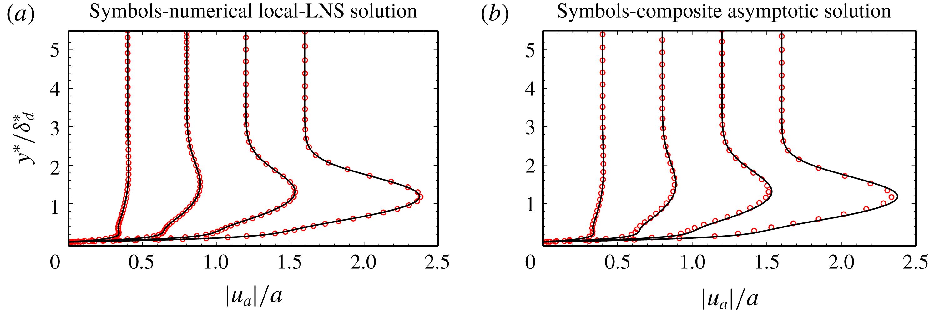
Acoustic streamwise velocity perturbation profiles scaled by $a=1/M_{\infty }$ (from left to right, $M_{\infty }=\{0.4,0.8,1.2,1.6\}$ , $\unicode[STIX]{x1D714}^{\ast }\bar{\unicode[STIX]{x1D708}}_{\infty }/\bar{U}_{\infty }^{2}\times 10^{6}=\{1.120,0.985,0.876,0.794\}$ and $R=70.2\times 10^{6}$ ).  $\unicode[STIX]{x1D6FF}_{d}^{\ast }$ represents the boundary layer displacement thickness. Black solid lines – numerical LUBLE solution.

The steady adjoint computation is a forced problem and thus needs to be addressed differently than the homogeneous problem at the inflow. At this streamwise position, we approximate the AHLNS with the local adjoint linearised Navier–Stokes (LNS) by introducing

(3.6) $$\begin{eqnarray}\tilde{\boldsymbol{q}}_{s,w}(x,y)=\tilde{\boldsymbol{q}}_{s,w}(y)\text{e}^{\text{i}(-\unicode[STIX]{x1D6FC}_{1}+\unicode[STIX]{x1D6FC}_{a})x},\end{eqnarray}$$

whereas at the outflow we impose

(3.7) $$\begin{eqnarray}{\displaystyle \frac{\unicode[STIX]{x2202}\tilde{\boldsymbol{q}}_{s,w}}{\unicode[STIX]{x2202}x}}=\text{i}(-\unicode[STIX]{x1D6FC}_{2}+\unicode[STIX]{x1D6FC}_{a})\tilde{\boldsymbol{q}}_{s,w}.\end{eqnarray}$$

4.1 Stokes layer

The T–S wave solution is very sensitive to changes in the Stokes layer. Therefore it is important to guarantee an accurate representation of this field. For validation we introduce the ansatz

(4.1) $$\begin{eqnarray}\boldsymbol{q}_{a}(x,y)=\hat{\boldsymbol{q}}_{a}(y)\text{e}^{\text{i}\unicode[STIX]{x1D6FC}_{a}x},\end{eqnarray}$$

into the homogeneous HLNS equations and solve for $\hat{\boldsymbol{q}}_{a}(y)$ with appropriate boundary conditions. The resulting governing equations, henceforth denoted local LNS, are similar to the compressible linear stability equations, but with the non-parallel steady base flow terms retained in the equation set.

In figure 1(a) we compare numerical solutions of the LUBLE and of the local-LNS approaches for Mach numbers ranging from low subsonic to moderate supersonic regimes; very good agreement between the two approaches is evident. In figure 1(b) we replicate the same flow conditions and compare the LUBLE with the high Strouhal number asymptotic solution (2.24). Good agreement is found, with only minor differences between the two radically different treatments. These differences are more noticeable in an overlap region due to the matching of the inner and outer layer solutions, neither of which are strictly valid there.

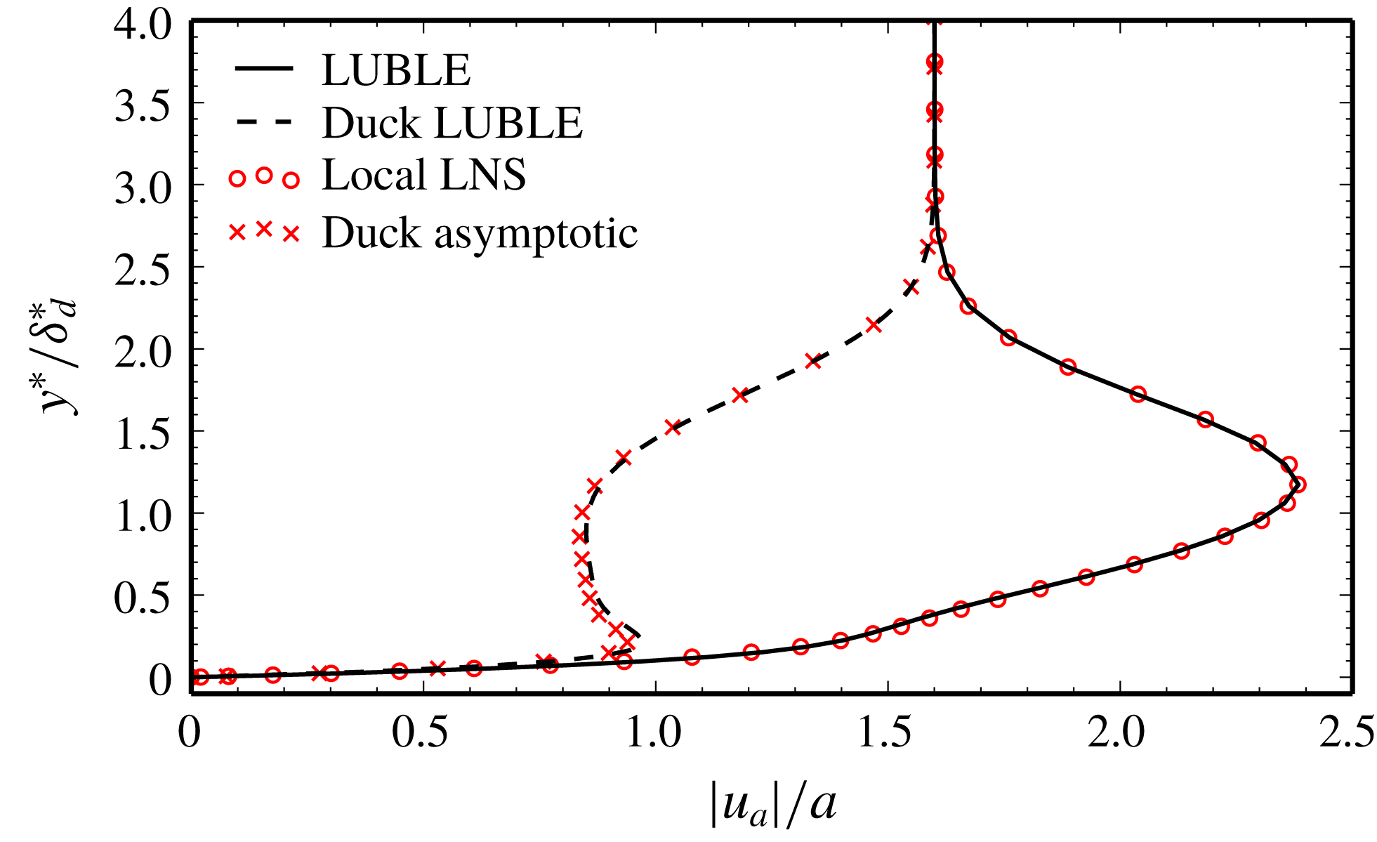
Lastly, we perform a comparison between the LUBLE numerical solution and the asymptotic solution of Duck (Reference Duck1990) in figure 2. In addition, we have replaced the governing equations of the LUBLE solver with those presented by Duck (Reference Duck1990) and computed a numerical solution (denoted ‘Duck LUBLE’ in the legend). On the one hand, there is good agreement between the asymptotic solution of Duck and the numerical solution of the corresponding governing equations. This indicates that this asymptotic solution is correctly deduced. On the other hand, there is a mismatch between the solutions of the two different equation sets, both analytical and numerical. This implies that the equation sets themselves are not equivalent. Duck deduced the LUBLE by linearising the unsteady form of (2.6). While this route should be equivalent to the one taken in the present work, it appears that the time fluctuation of the ‘independent’ variable $\unicode[STIX]{x1D702}$ was not taken into account.

Figure 2.

Acoustic streamwise velocity perturbation profile ( $M_{\infty }=1.6$ , $\unicode[STIX]{x1D714}^{\ast }\bar{\unicode[STIX]{x1D708}}_{\infty }/\bar{U}_{\infty }^{2}\times 10^{6}=0.794$ and $R=70.2\times 10^{6}$ ). Comparison between the present approach and Duck (Reference Duck1990).

4.2 Comparison with asymptotic theory and DNS

De Tullio & Ruban (Reference De Tullio and Ruban2015) compared triple-deck-based receptivity theory with DNS computations. Two types of wall perturbations were considered – Gaussian-shaped roughness elements and vibrating ribbons. This brief comparison with their work focuses on linear receptivity caused by localised surface roughness.

The test case consists of a Gaussian-shaped bump placed on an adiabatic flat plate at $x^{\ast }=L_{b}$ and an acoustic wave propagating downstream with non-dimensional frequency $F_{n}=f^{\ast }\bar{\unicode[STIX]{x1D707}}_{\infty }/\bar{\unicode[STIX]{x1D70C}}_{\infty }\bar{U}_{\infty }^{2}$ such that the first branch of neutral stability (B-I) coincides with the roughness position. We define the Reynolds number $R_{b}=L_{b}\bar{U}_{\infty }/\bar{\unicode[STIX]{x1D708}}_{\infty }$ . The Gaussian shape is described by

(4.2) $$\begin{eqnarray}\widehat{H}(x)=\exp \left[-{\displaystyle \frac{(x-x_{b})^{2}}{2(\unicode[STIX]{x1D6E5}/6)^{2}}}\right],\end{eqnarray}$$

where $\unicode[STIX]{x1D6E5}$ is the non-dimensional Gaussian shape width and $x_{b}=L_{b}/L$ . See table 1 of TR for a full definition of the test cases under analysis.

Our computational domain extends for approximately 30 T–S wavelengths and no less than 200 points per wavelength are used in the streamwise direction. In the wall-normal direction we use 62 Chebyshev polynomials. The results were checked to be grid independent to graphical precision, in other words finer meshes would give graphically indistinguishable results.

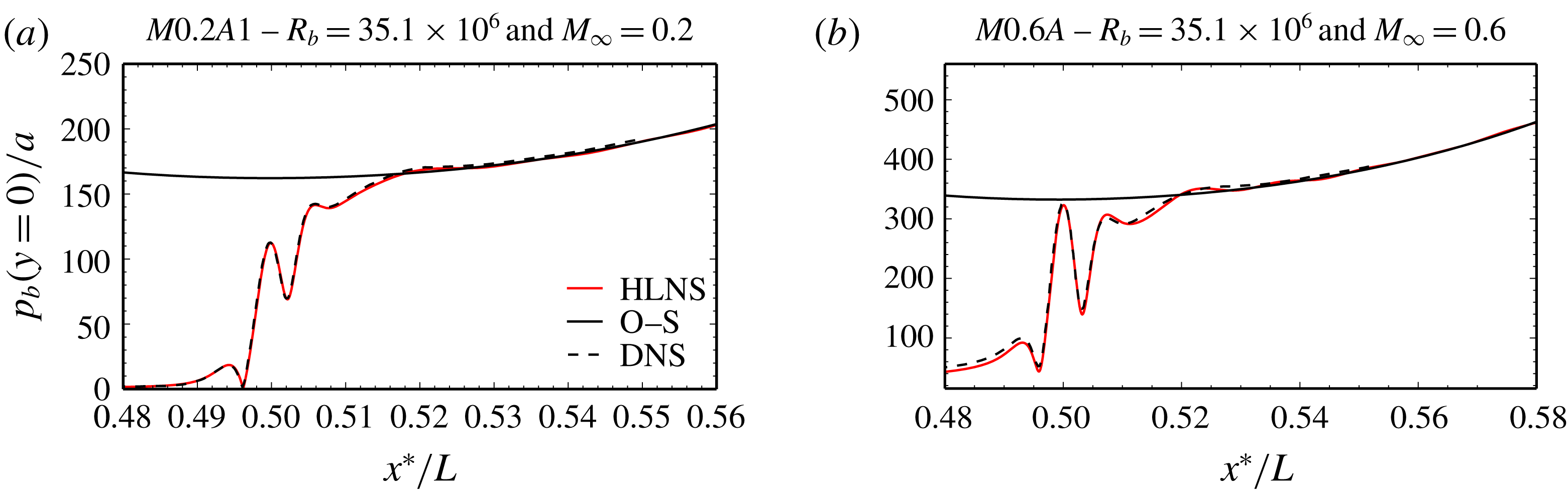
In figure 3 we present a quantitative comparison between the HLNS approach proposed in this paper and the DNS of TR. The wall-pressure perturbation amplitude $p_{b}(x,y=0)$ of the T–S wave is plotted against the streamwise position for test cases $M0.2A1$ and $M0.6A$ . Remarkable quantitative agreement is observed not only in the T–S dominated region downstream of the roughness element, which is positioned at $x_{b}=0.5$ , but especially so in the resonance interaction region. This highlights the DNS-like accuracy of the present approach, having used significantly less computational resources. While the precise duration is case dependent, a typical computation requires a total time of order 15 min using 20 cores. This strongly contrasts with the large computational times and computational power required to perform a study similar to that of TR. A more detailed comparison can be found in Raposo, Mughal & Ashworth (Reference Raposo, Mughal and Ashworth2018b ).

Figure 3.

T–S wave wall-pressure amplitude evolution along the flat plate – comparison between HLNS, compressible O–S and TR’s DNS. $\unicode[STIX]{x1D6E5}/\unicode[STIX]{x1D706}_{\text{TS}}=1$ , where $\unicode[STIX]{x1D706}_{\text{TS}}$ is the T–S wavelength at the centre of the Gaussian bump.

4.3 Adjoint HLNS comparison with finite Reynolds number theory (FRNT)

Choudhari (Reference Choudhari1994) extended finite Reynolds number theory (Choudhari & Streett Reference Choudhari and Streett1992) to compressible flows and proceeded to study receptivity in the presence of localised suction and heating strips. The author addressed the acoustic-field signature problem using the compressible O–S equations with appropriate boundary conditions (forcing theory (Mack Reference Mack1984)), although scant details are provided concerning the exact form of the governing equations and of the adopted numerical procedures to account for wave reflection. Nonetheless, Choudhari’s approach takes into account the presence of the boundary layer and the effect of viscosity on the reflection and refraction process. This method contrasts with the thin boundary layer approximation employed in this paper, wherein the inviscid acoustic flow and the viscous boundary layer acoustic signature are treated separately. The main goal in the analysis that follows is thus to establish the extent to which the LUBLE can be used as an approximation to determine the acoustic-field signature in the boundary layer, and how the accuracy of this approximation varies with Mach number and angle of incidence.

Consider a localised, uniform-profile, suction strip centred at $\sqrt{R_{b}}=955$ and an incoming acoustic wave incident on the flat plate at an angle $\unicode[STIX]{x1D6E9}$ . The acoustic wave frequency is such that B-I coincides with the centre of the strip. An adiabatic wall condition is used with a constant stagnation temperature of 311 K for all cases. The numerical domain extends from $\sqrt{R_{b}}=423$ to $\sqrt{R_{b}}=1640$ , although in the interval $\sqrt{R_{b}}=423{-}733$ the solution is damped by means of a sponge layer to avoid spurious reflections. In the streamwise direction we employ 8000 points (approximately 200 points per T–S wavelength), whereas 62 Chebyshev polynomials are used in the wall-normal direction. This grid was confirmed to yield converged results up to graphical precision.

We seek to establish a comparison with figure 2(a–c) in Choudhari (Reference Choudhari1994). This involves calculating the so-called efficiency function based on the maximum of the streamwise mass-flux perturbation normalised by the acoustic wave pressure amplitude

(4.3) $$\begin{eqnarray}|\unicode[STIX]{x1D6EC}_{\unicode[STIX]{x1D70C}U,p}^{(j)}|=\max _{y}{\displaystyle \frac{|(\bar{U}\unicode[STIX]{x1D70C}_{b}+\bar{\unicode[STIX]{x1D70C}}u_{b})(x_{b},y)|}{|{\mathcal{F}}(\unicode[STIX]{x1D6FC}_{w})|p_{a,\infty }}},\end{eqnarray}$$

where $\unicode[STIX]{x1D6FC}_{w}=\unicode[STIX]{x1D6FC}_{\text{TS}}(x_{b})-\unicode[STIX]{x1D6FC}_{a}$ and ${\mathcal{F}}(\unicode[STIX]{x1D6FC})$ is the Fourier transform of the wall inhomogeneity profile. For a uniform-profile strip it assumes the form

(4.4) $$\begin{eqnarray}{\mathcal{F}}(\unicode[STIX]{x1D6FC})={\displaystyle \frac{1}{\unicode[STIX]{x1D6FC}}}\sqrt{{\displaystyle \frac{2}{\unicode[STIX]{x03C0}}}}\sin \left({\displaystyle \frac{\unicode[STIX]{x1D6FC}d}{2}}\right),\end{eqnarray}$$

where $d$ is the width of the suction strip. The reference length scale is the boundary layer displacement thickness at the centre of the suction strip. The instability amplitude at B-I is extracted by means of matching with a PSE solution

(4.5) $$\begin{eqnarray}(\bar{U}\unicode[STIX]{x1D70C}_{b}+\bar{\unicode[STIX]{x1D70C}}u_{b})(x_{b})={\displaystyle \frac{(\bar{U}\unicode[STIX]{x1D70C}_{b}+\bar{\unicode[STIX]{x1D70C}}u_{b})(x_{m})}{\exp \left[-\displaystyle \int _{x_{b}}^{x_{m}}\text{Im}(\unicode[STIX]{x1D6FC}_{\text{TS}})\,\text{d}\unicode[STIX]{x1D709}\right]}},\end{eqnarray}$$

where $x_{m}$ denotes the matching streamwise coordinate. The efficiency function is a natural quantity to compare different receptivity theories under the parallel flow assumption due to its independence of the wall-disturbance profile. For a finite-sized strip in non-parallel flows, the definition proposed in (4.3) is not strictly valid. In practice however, the efficiency function will converge to graphical precision provided the width of the suction strip is sufficiently small.

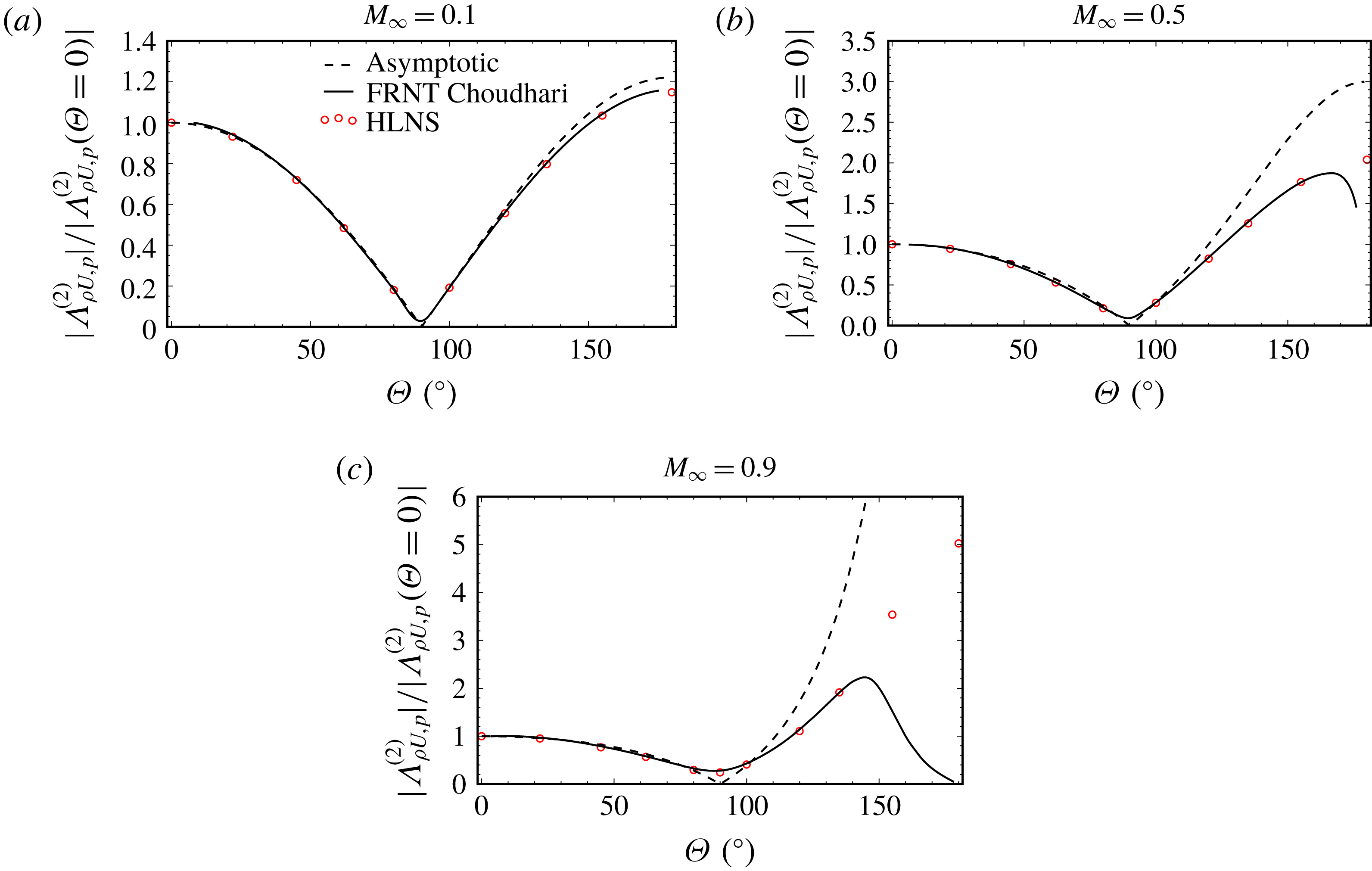
In figure 4 we assess the influence of the acoustic wave angle of incidence on the efficiency function (4.3). For each Mach number this quantity is normalised by its value at $\unicode[STIX]{x1D6E9}=0^{\circ }$ . The triple-deck-based asymptotic prediction (Ruban Reference Ruban and Kozlov1985) is then simply the ratio between the Stokes layer amplitudes as given by (2.23a ), namely

(4.6) $$\begin{eqnarray}{\displaystyle \frac{|\unicode[STIX]{x1D6EC}_{\unicode[STIX]{x1D70C}U,p}^{(j)}(\unicode[STIX]{x1D6E9})|}{|\unicode[STIX]{x1D6EC}_{\unicode[STIX]{x1D70C}U,p}^{(j)}(\unicode[STIX]{x1D6E9}=0)|}}={\displaystyle \frac{|\text{cos}(\unicode[STIX]{x1D6E9})(1+M_{\infty })|}{|1+M_{\infty }\text{cos}(\unicode[STIX]{x1D6E9})|}},\end{eqnarray}$$

and represented with dashed black lines in figure 4. This simple correlation always has a maximum for $\unicode[STIX]{x1D6E9}=180^{\circ }$ , i.e. for an upstream propagating wave. We also present numerical results obtained with the LUBLE-based model described in this work, as well as the results published by Choudhari (Reference Choudhari1994).

Figure 4.

Efficiency function ratio against the acoustic wave angle of incidence for a suction strip wall mechanism. The legend of panel (a) is valid for all panels.

Remarkable agreement is found between asymptotic theory, forcing theory and a LUBLE-based approach at shallow angles of incidence. At fixed Mach number and increasing angle of incidence, we initially observe a departure of the asymptotic prediction from the still-in-agreement LUBLE and forcing theory. As the angle increases further, the LUBLE and forcing theory results begin to deviate. The deviation between the two approaches increases with growing Mach number.

Therefore, for any given Mach number there is an interval of angles of incidence for which the LUBLE-based approach and forcing theory agree, but wherein asymptotic theory predicts significantly different receptivity levels. This is in direct contradiction with Choudhari’s explanation for the deviation of the efficiency function from the asymptotic prediction. He argued that this could be explained by non-trivial sound wave refraction patterns and variations in the acoustic pressure field across the boundary layer. While this argument is still a prime candidate to explain the efficiency function dip for angles near $180^{\circ }$ , it cannot explain the inaccuracy of the asymptotic prediction at more moderate angles of incidence because the numerical LUBLE solution also does not account for this phenomenon and yet continues to be a reliable approximation. This behaviour indicates that the efficiency function has a non-trivial dependency on the form of the Stokes layer (see chapter 3 of Bernots (Reference Bernots2014)).

Forcing theory predicts a sudden decrease in receptivity at high angles of incidence, near $\unicode[STIX]{x1D6E9}=180^{\circ }$ . This trend starts to become evident at ever-smaller angles of incidence as the Mach number increases. According to Brand & Nagel (Reference Brand and Nagel1982), as one approaches $\unicode[STIX]{x1D6E9}=180^{\circ }$ the acoustic waves are refracted away from the wall and hence the acoustic-field boundary layer signature is weakened. This effect is all the more pronounced as the Mach number increases and explains the decreasing receptivity levels at high angles of incidence.

In conclusion, the LUBLE are a good approximation across the subsonic Mach number and angle of incidence parameter space, except for a band of angles for near upstream propagating waves. As the Mach number increases, use of the LUBLE model becomes questionable for an increasing range of incidence angles, for which viscous refraction should be taken into account. Non-parallel flow effects are relatively unimportant for the studied conditions.

Table 1.

Parametric study conditions – Mach number, frequency and T–S wave orientation.

4.4 Efficiency function

In this section the computational advantage afforded by the AHLNS is exploited to quantify the efficiency function for a range of frequencies, Mach numbers, spanwise wavenumbers, Reynolds numbers and wall perturbation mechanisms. The adjoint provides a means to obtain the receptivity sensitivity with respect to the latter two parameters virtually instantaneously.

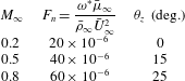
The range of Mach numbers, frequencies and T–S wave orientations considered is presented in table 1. The angle $\unicode[STIX]{x1D703}_{z}$ refers to the T–S wave orientation at the location of B-I as measured through the maximum streamwise mass flux. For conciseness, results for every possible combination of the parameter space are not presented. Instead, we start by analysing the effects of Mach number and frequency for 2-D T–S waves ( $\unicode[STIX]{x1D703}_{z}=0^{\circ }$ ). We then proceed to select one Mach number and wall actuation mechanism to analyse the effect of T–S wave obliqueness on the efficiency function for each frequency. Lastly, we evaluate how receptivity to oblique T–S waves varies with Mach number for a single frequency.

The quantity used to assess receptivity is not the efficiency function in its classical sense, where amplitudes are scaled back to the location of the wall inhomogeneity (Choudhari Reference Choudhari1994). Instead, we choose to perform backtracking to the first branch of neutral stability $x_{I}$ to provide a fairer comparison of amplitudes obtained for different locations of the wall perturbation. Mathematically, we evaluate

(4.7) $$\begin{eqnarray}|\unicode[STIX]{x1D6FA}_{\unicode[STIX]{x1D70C}U,\unicode[STIX]{x1D70C}U}^{(j)}|(x_{b})={\displaystyle \frac{(2\unicode[STIX]{x03C0})^{1/2}}{(\unicode[STIX]{x1D70C}u)_{a,\infty }}}A_{\unicode[STIX]{x1D70C}U}(x_{I})|A_{2}|(\widehat{H}(x)=\unicode[STIX]{x1D6FF}(x-x_{b})),\end{eqnarray}$$

where $A_{\unicode[STIX]{x1D70C}U}$ is the maximum amplitude of the streamwise mass-flux perturbation and $\left(\unicode[STIX]{x1D70C}u\right)_{a,\infty }=\text{cos}(\unicode[STIX]{x1D6E9})+M_{\infty }$ . The efficiency function is thus the T–S wave amplitude produced by a Dirac delta forcing $\unicode[STIX]{x1D6FF}(x-x_{b})$ evaluated through (2.36). We use the local boundary layer displacement thickness ( $x=x_{b}$ ) as a reference length scale, thus defining a local Reynolds number $R_{\unicode[STIX]{x1D6FF}}$ . An adiabatic wall condition is used with a constant stagnation temperature of 311 K for all cases.

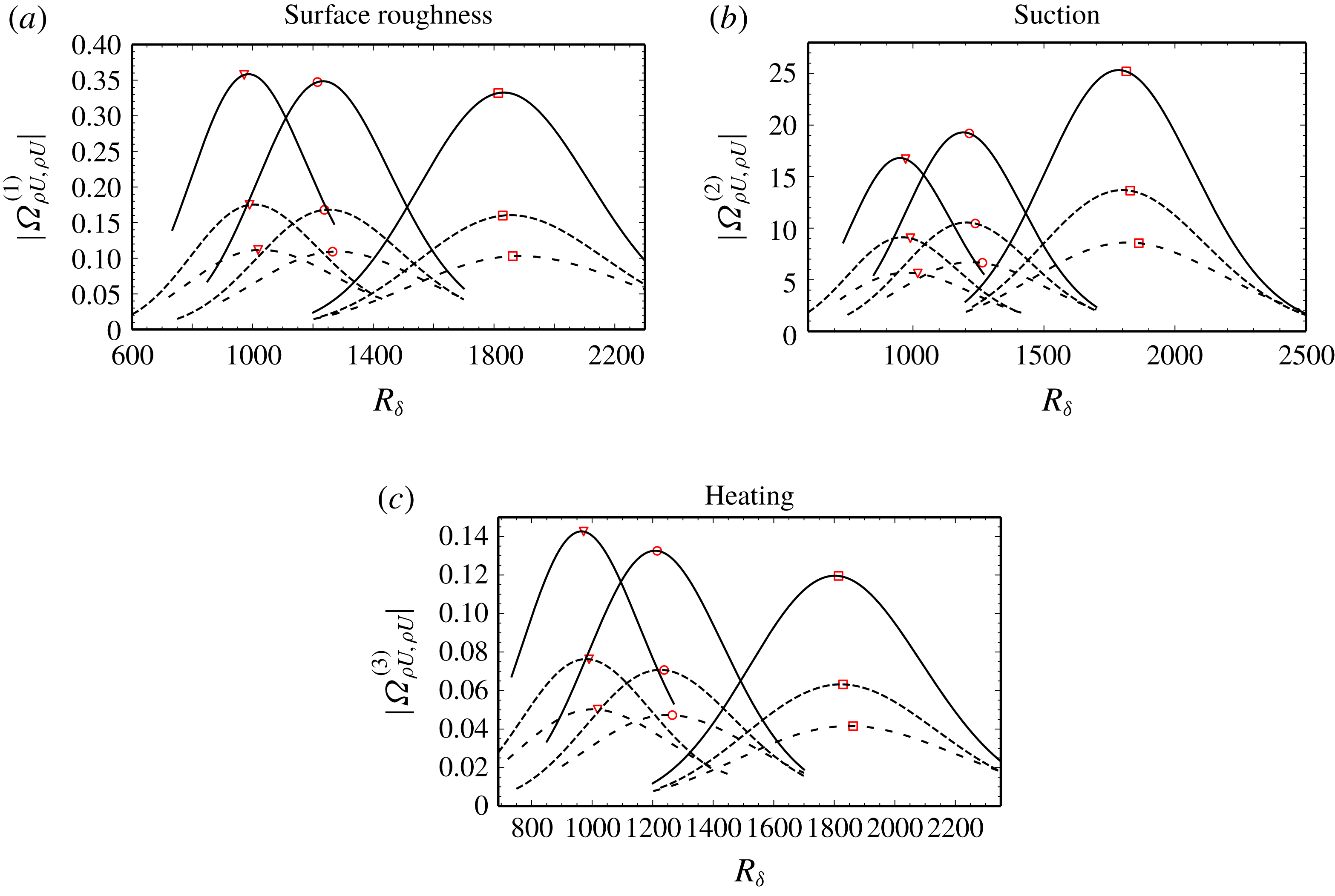
Figure 5 presents the efficiency function for 2-D T–S modes for all Mach numbers, frequencies and wall actuation mechanisms considered. The plots show the evolution of the efficiency function with the position of the wall inhomogeneity and highlight the location of the first branch of stability. For surface roughness at a fixed Mach number, a small increase in efficiency with the acoustic wave frequency is observed. This behaviour is identical at all Mach numbers. A similar trend is observed for wall heating, although the increase in efficiency with acoustic frequency is more pronounced. On the other hand, suction devices present an opposite trend. Note also how the maximal T–S amplitude is obtained if a roughness element is placed just downstream of B-I, whereas for suction and heating the optimal location occurs slightly upstream of this point. The boundary layer is receptive to lower acoustic frequencies in a large portion of the domain, but on the other hand higher frequencies influence the flow much further upstream. Lastly, for a fixed frequency, a decrease in efficiency for increasing free-stream Mach number occurs. However, it is worth noting that this trend is closely related to the choice of flow quantity used to define the T–S and acoustic wave amplitudes.

Figure 5.

Efficiency function in function of local Reynolds number for different Mach numbers, frequencies and wall-disturbance mechanisms. $\unicode[STIX]{x1D703}_{z}=0^{\circ }$ ; solid curves – $M_{\infty }=0.1$ ; short dashed curves – $M_{\infty }=0.5$ ; long dashed curves – $M_{\infty }=0.8$ ; symbols – B-I location; square – $F_{n}=20\times 10^{-6}$ ; circle – $F_{n}=40\times 10^{-6}$ ; triangle – $F_{n}=60\times 10^{-6}$ .

Figure 6.

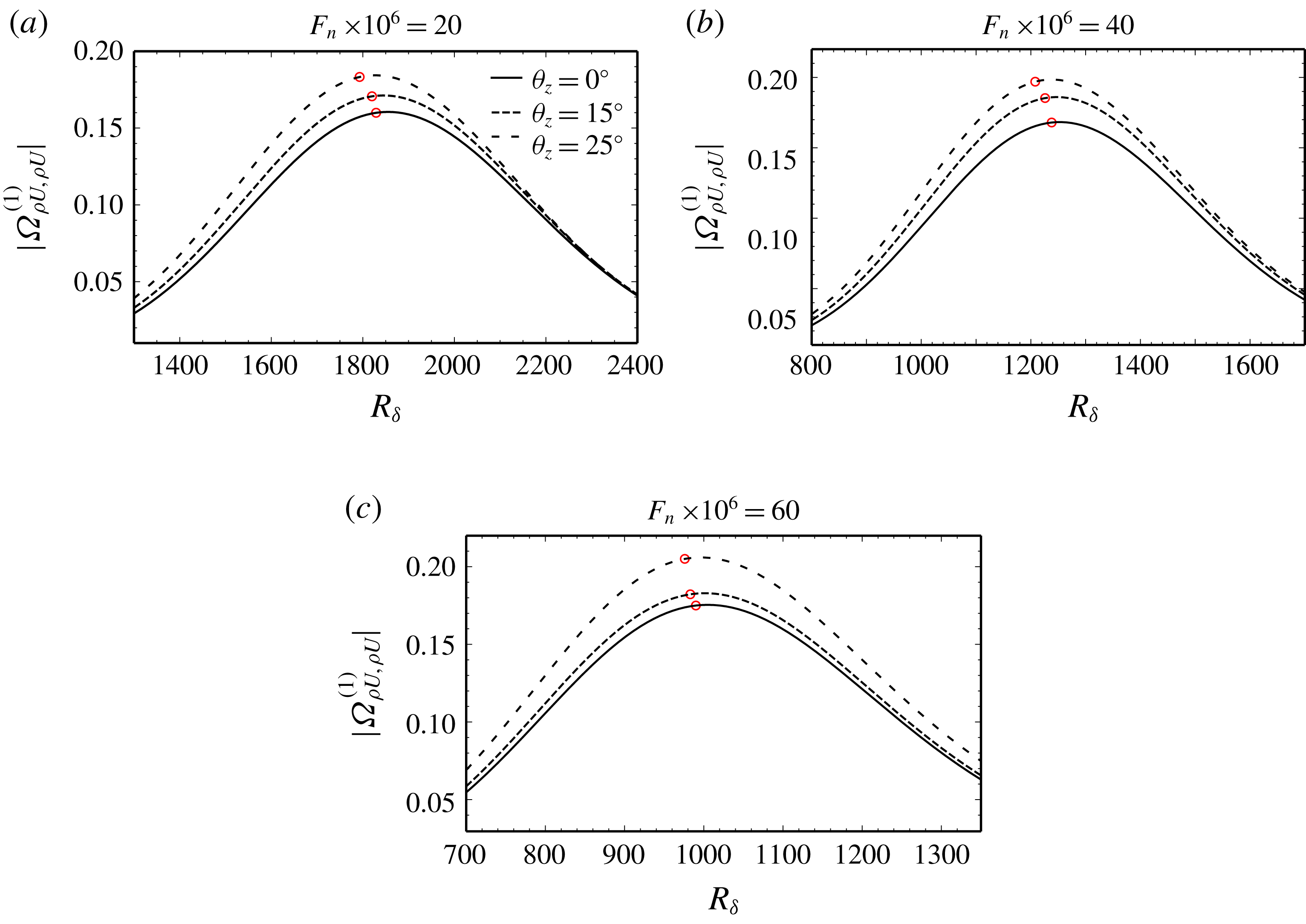
Surface roughness efficiency function in function of local Reynolds number for different frequencies and spanwise wavenumbers at fixed Mach number $M_{\infty }=0.5$ . Red circle – B-I location.

In figure 6 the free-stream Mach number is held constant at $M_{\infty }=0.5$ and focus is on surface roughness. For each acoustic frequency, we plot the efficiency function for three different T–S wave orientations. The results are consistent with what has previously been observed in the incompressible regime (Crouch & Bertolotti Reference Crouch and Bertolotti1992; Raposo et al. Reference Raposo, Mughal and Ashworth2018a ) – the boundary layer is more receptive to oblique disturbances than to 2-D instabilities across the frequency parameter space. Although not presented here, a similar effect is observed for suction and heating. Conversely, for incompressible flow it is known that 2-D modes are more unstable than their oblique counterparts. However, as the Mach number increases, oblique first modes become the dominant instability (El-Hady Reference El-Hady1991). 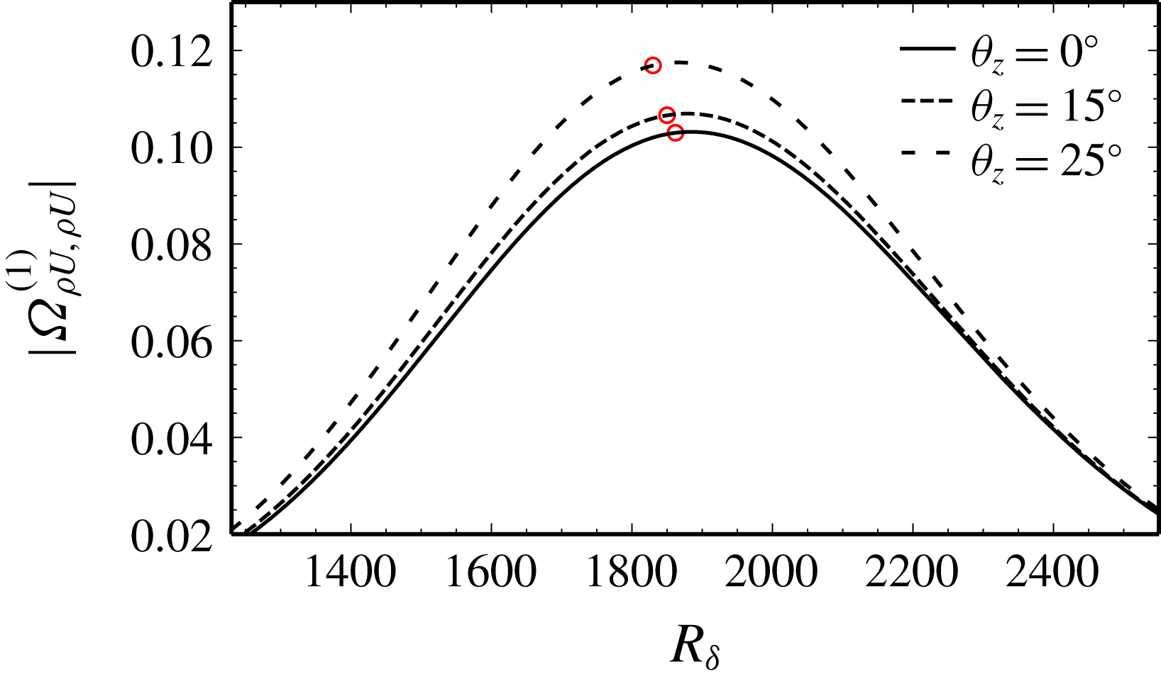At $M_{\infty }=0.5$ this is still not the case, but at $M_{\infty }=0.8$ , both disturbances with $\unicode[STIX]{x1D703}_{z}=15^{\circ }$ and $\unicode[STIX]{x1D703}_{z}=25^{\circ }$ present higher amplification than those of the 2-D disturbance for $F_{n}=20\times 10^{-6}$ (not shown). Nonetheless, in figure 7 we observe that no similar inversion in trends occurs for receptivity, wherein oblique disturbances continue to be the most receptive. This indicates that linear growth at high subsonic and transonic Mach numbers may be dominated by 3-D disturbances because they are both more receptive to external disturbances and more unstable than their 2-D counterparts.

Figure 7.

Surface roughness efficiency function in function of local Reynolds number for different spanwise wavenumbers at fixed Mach number $M_{\infty }=0.8$ and frequency $F_{n}=20\times 10^{-6}$ . Red circle – B-I location.